Modeling the Impact of Climate Change on Water Availability in the Zarrine River Basin and Inflow to the Boukan Dam, Iran


Department of Geohydraulics and Engineering Hydrology, University of Kassel, 34125 Kassel, Germany
*
Author to whom correspondence should be addressed.
Climate 2019, 7(4), 51; https://0-doi-org.brum.beds.ac.uk/10.3390/cli7040051
Submission received: 1 December 2018
/
Revised: 15 March 2019
/
Accepted: 18 March 2019
/
Published: 3 April 2019
Abstract
:The impacts of climate change on the water availability of Zarrine River Basin (ZRB), the headwater of Lake Urmia, in western Iran, with the Boukan Dam, are simulated under various climate scenarios up to year 2029, using the SWAT hydrological model. The latter is driven by meteorological variables predicted from MPI-ESM-LR-GCM (precipitation) and CanESM2-GCM (temperature) GCM models with RCP 2.6, RCP 4.5 and RCP 8.5 climate scenarios, and downscaled with Quantile Mapping (QM) bias-correction and SDSM, respectively. From two variants of QM employed, the Empirical-CDF-QM model decreased the biases of raw GCM- precipitation predictors particularly strongly. SWAT was then calibrated and validated with historical (1981–2011) ZR-streamflow, using the SWAT-CUP model. The subsequent SWAT-simulations for the future period 2012–2029 indicate that the predicted climate change for all RCPs will lead to a reduction of the inflow to Boukan Dam as well as of the overall water yield of ZRB, mainly due to a 23–35% future precipitation reduction, with a concomitant reduction of the groundwater baseflow to the main channel. Nevertheless, the future runoff-coefficient shows a 3%, 2% and 1% increase, as the −2% to −26% decrease of the surface runoff is overcompensated by the named precipitation decrease. In summary, based on these predictions, together with the expecting increase of demands due to the agricultural and other developments, the ZRB is likely to face a water shortage in the near future as the water yield will decrease by −17% to −39%, unless some adaptation plans are implemented for a better management of water resources.
1. Introduction
Fresh water uses are expected to increase significantly in the coming years, owing to population growth, increased urbanization and agricultural development. The “Comprehensive Assessment of Water Management in Agriculture” reveals that one in three people in the world is already facing severe water shortages [1]. This holds particularly for the Mediterranean and arid climate zone across the northern hemisphere. For example, recent NASA satellite studies reveal that parts of the arid Middle East region and western Iran lost freshwater reserves rapidly over the past decade, which means that Iran will be facing a serious and protracted water shortage [2]. This water scarcity is aggravated by increased climate variability due to global climate change reflected by droughts with drying lakes and rivers, declining groundwater resources and deteriorating water quality in the country [3].
As global warming is expected to intensify in the 21st century, further hydro-climatic disasters, namely, water scarcity in the form of droughts, are to be anticipated. Since climate change impacts will not only reduce the available water resources, but also increase the water demands by crops, i.e., will negatively impact agricultural production [4], the first unavoidable step to prepare affected societies for this water shortage and to evaluate these adverse water resources impacts, is the identification of the climate variations, followed by a prediction of the hydro-climatic conditions for the future.
Numerous publications deal with the assessment of regional climate change impacts on available water resources in Iran and other countries (e.g., [5,6,7]). However, fewer studies focused on the evaluation of streamflow changes, let alone to apply the further step which is to manage the available regional water resources under changing future climate scenarios [8,9]. The novelty of this research lies in transferring the large scale GCM-based climate signals to the local hydrologic cycle changes and in predicting the future hydrological components and the available water resources of a river basin in a semi-arid region from the simulation of the inflow to a main reservoir.
With the above background at hand, this paper aims to assess the impacts of climate change on the hydrological characteristics of the Zarrine River Basin (ZRB) with the Boukan Dam located in northwest Iran. The Zarrine River (ZR) is the main inflow source of Lake Urmia, which is the largest inland wetland of Iran and the largest lake in the Middle East [10]. In fact, recent publications (e.g., [11]) indicate that the Aral Sea syndrome desiccates also Lake Urmia—located in the vicinity of the present study region—so that the area of this Iranian lake has decreased by around 88% in the past several decades. In fact, Lake Urmia’s water body, which has an international importance based on the Ramsar convention, has been diminishing steadily since 1995. Based on these facts, it has been argued that the current condition of Lake Urmia necessitates immediate action to avoid an environmental and ecological disaster. The significant shrinkage in the lake’s surface area is not only due to prolonged droughts in recent years, but also a consequence of the aggressive regional water resources development plans, unsustainable agricultural activities, anthropogenic changes of the system and upstream stakeholder competition over water in the upstream areas, i.e. the ZRB [7].
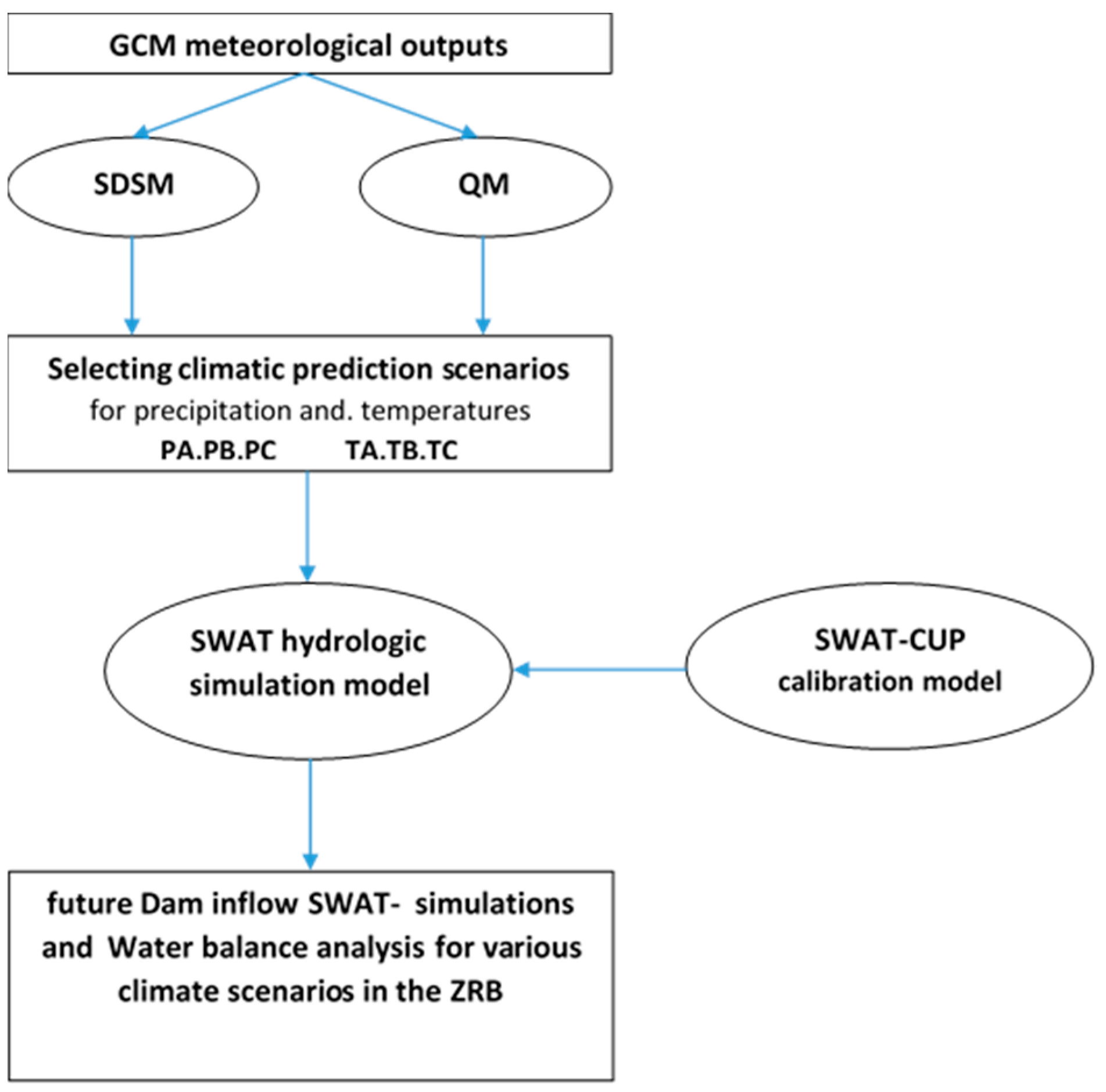
In the present study, future GCM climate projections of temperatures and precipitation under different climate scenarios are downscaled for use as input in a hydrologic watershed model (SWAT) to simulate the ZRB’s water resources’ response to the impacts of a changing climate. Particular emphasis will be laid on the prediction of the Boukan Dam’s future inflow changes, as this reservoir stores much of the region’s surface water for satisfying the various water needs there. The flowchart of the study steps is outlined in Figure 1.
2. Study Area
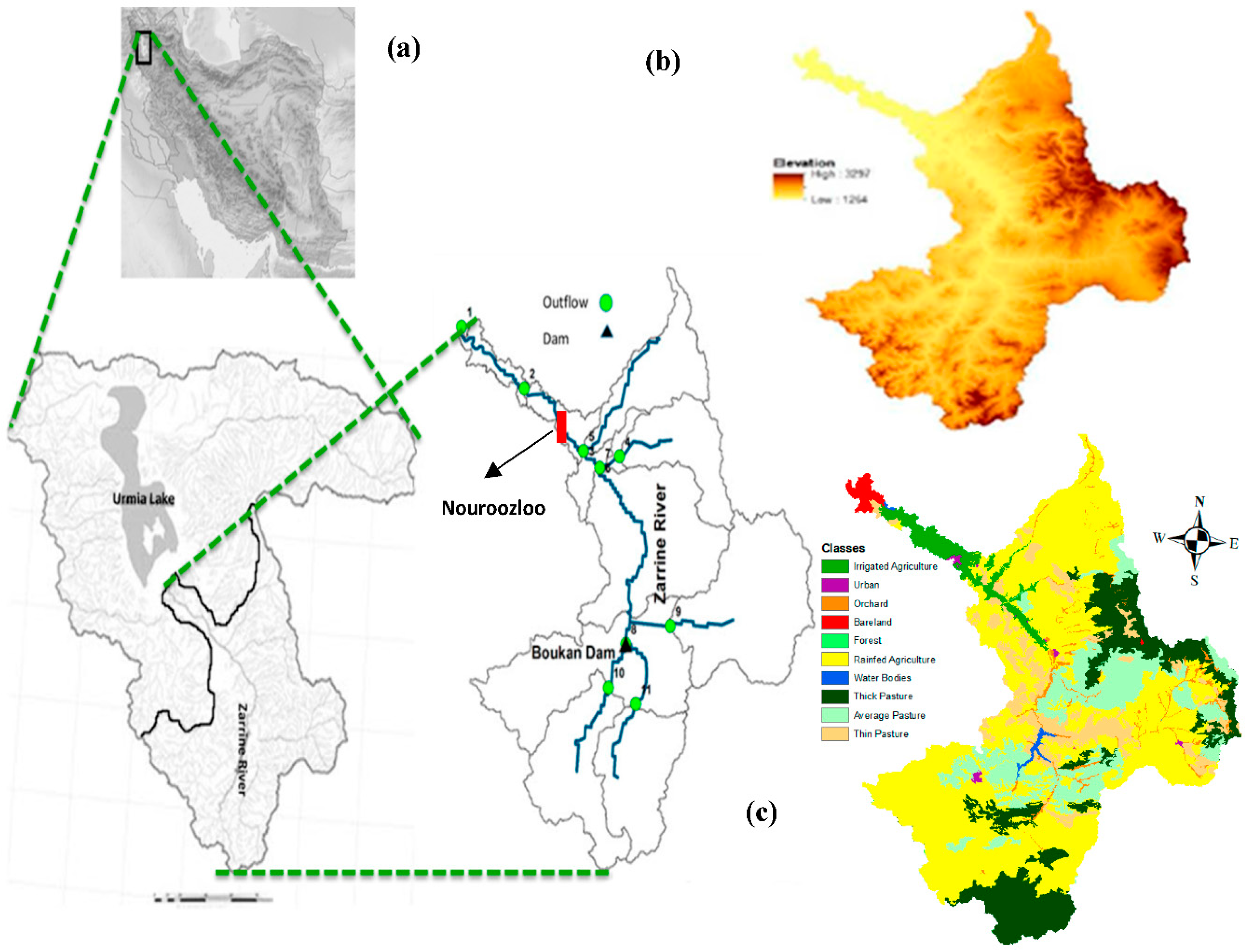
The ZRB, located between 45°46′ E to 47°23′ W longitude and 35°41′ S to 37°44′ N latitude, forms the southern sub-basin of the Lake Urmia catchment and covers an area of about 11,000 km2 (see Figure 2a). The ZR itself has a total length of about 300 km and most of its course is within a mountainous area. The ZRB belongs to the Lake Urmia hydrologic basin which is one of the six main basins in Iran. Up until recent times, the ZR flowed directly into Lake Urmia; however, with the more recent drying trend, the lake has retreated by about 30 km from the river’s mouth.
The reservoir system in the ZRB contains three operating dams and one diversion dam, together with 24 hydrometrical stations. The ZR’s headwaters pour out from the Kurdestan Chelchshme Mountains, pass through deep valleys in the northern direction and flow into the Lake Urmia. The main branches of the ZR are named Chamkhorkhore, Saghezchay and Saroghchay. The first two join near Pol-gheslagh and then Saroghchay joins them at the most important dam of the basin, the Boukan reservoir dam, the only dam located on the Zarrine River and serving with a storage capacity of 650 MCM much of the region’s needs of potable and agriculturally used water. The discharge of the dam continues to flow towards the North, while intersecting the three rivers Joshatosofla, Ajorlochay and Ghoorichay. Then, the river enters the Norouzloo diversion dam and finally discharges into Lake Urmia.
The region’s climate is mostly characterized as semi- wet cold or wet- cold in the mountain areas with annual precipitation of up to 800 mm/yr, but changes to semi- dry in the vicinity of Lake Urmia where the precipitation is only about 200 mm/yr. The major land cover of the basin is 45% dry land, 37% pasture and 14% forest (see Figure 2c). The ZRB is rather prone to flooding and devastating floods have occurred there in recent years, especially, in the beginning of the spring, when snow melt in the mountain areas of the basin occurs.
3. Materials and Methods
3.1. Hydrological Simulation Model SWAT
3.1.1. Theoretical Concepts of the SWAT-Model
The Soil and Water Assessment Tool (SWAT) is a physically-based integrated semi-distributed hydrological model that has originally been developed to mainly simulate the impacts of land management practices in large and complex watersheds [12]. However, SWAT is also an efficient simulator of hydrology and water quality, so that it has increasingly being used to investigate climate change impacts on agro-hydrological systems [5,13]. In such applications, SWAT’s meteorological input drivers are usually downscaled climate predictors from GCM-models.
The watershed to be modeled is partitioned further into sub-basins to represent the large-scale spatial heterogeneity of the research area, and each sub-watershed is divided further into a set of HRUs (Hydrologic Response Units) which are a particular combination of land cover-, soil- and management- areal units. For each HRU in a sub-basin, soil water content, water and sediment yield, crop growth and the land management practices are simulated and then aggregated, based on the watershed slopes, reach dimensions, and other physical characteristics of the sub-basin. The streamflow of the sub-basins are estimated using the modified Soil Conservation Service (SCS) curve number method, routed by classic methods, and then accumulated through the river basin.
The simulated hydrological variables of the SWAT model are evapotranspiration, surface runoff, percolation, groundwater return flow, snowmelt, flow from shallow aquifers to streams, lateral subsurface flow, and channel transmission losses. The model inputs for the land- and other routing phases of the hydrologic cycle can be categorized as climate, hydrology, land cover, nutrients, pesticides and management practices. Required climate inputs for SWAT are min. and max. daily temperatures and precipitation as the ultimate climate drivers of the runoff process. The most important hydrologic and land cover model inputs include the physical characteristics of the watershed and sub-basins, i.e., soil type, land slope, slope lengths, Manning’s n-values (roughness coefficient) and characteristics of the surface water bodies. The remaining categories mentioned are not considered in this study and are thus not further discussed.
3.1.2. Model Setup
The required data for the SWAT-modelling were gathered from several sources. The network of rivers and the sub-basins of the watershed was delineated using the Digital elevation model (DEM) of the Iranian surveying organization, with a spatial resolution of 85 m (see Figure 2b), and the land use map of the watershed, with a resolution of 1000 m and 10 land use classes (see Figure 2c) was obtained from the Iranian Ministry of Jahade-Agriculture (MOJA) [14]. The soil map of the watershed was extracted from the FAO digital soil map of the world, with a spatial resolution of 10 km, and includes 8 types of soil with two layers for the study area. The land management practices and irrigation plans of the crops in ZRB are defined based on Ahmadzadeh et al. [15].
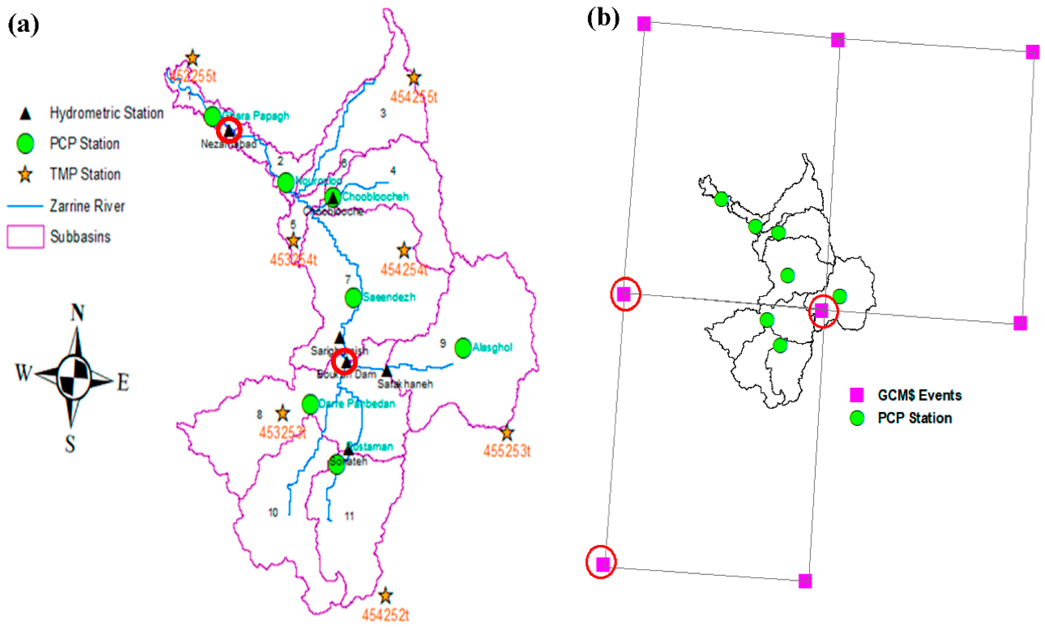
The climate input data contain daily precipitation of 21 stations obtained from the Iran Ministry of Energy (MOE), from which 7 representative stations (excluding other stations with longer and continuous data gaps) are selected, as shown in Figure 3. It should be noted that the model will assign precipitation for each sub-basin only from the nearest rain gauge to its centroid. In addition, because of a lack of temperature observations, GCM- predicted (on a 0.5° × 0.5° grid) daily max. and min. temperatures obtained from the Climate Research Unit (CRU) of the University of East Anglia, England, for the nearest 7 grid points (CRU stations) around or in the watershed over a period of 36 years (1977–2012) are used (see Figure 2a). River discharge data for 7 hydrometric stations, located at the outlets of the most important and effective sub-basins of the SWAT model (see Figure 2b) were obtained from MOE for the same period, whereas the reservoir’s monthly outflow was gathered from the IWRM Company, Tehran, Iran.
3.1.3. Calibration, Validation and Sensitivity Analysis
The recently developed SUFI-2 (Sequential Uncertainty Fitting) embedded in the SWAT-CUP (Calibration and Uncertainty Program) [16,17] was used for the calibration (parameter optimization), and sensitivity study of the SWAT-model. In SUFI-2/SWAT-CUP, users can investigate different objective functions and treat input data as near random parameters, i.e., model input parameters are expressed as ranges, accounting for all sources of uncertainties, due to parameter-, conceptual model-, input-, measured data- and other errors. In this method, a meaningful set of ranges is initially assigned to the calibrating parameters and then a set of samples are drawn from the ranges using Latin hypercube scheme, which divides the parameter ranges uniformly into N intervals (number of iterations) and randomly samples the values within the interval for each parameter. The uncertainty is quantified at the 2.5% and 97.5% levels of the cumulative frequency distribution of the simulated outputs which is referred to as the 95% prediction uncertainty (95PPU) [17,18]. Thus, the SUFI-2 algorithm differs from the classical deterministic Parameter Solution (ParaSol) method [19], used hitherto in most applications of SWAT [20].
The quality of the fit of the model output, namely, streamflow, to the observed one is also measured in SWAT-CUP by various quantities, such as the NSE, R2 (coefficient of determination) and RMSE (root-mean-square error) and a somewhat less used quantity, bR2. The latter takes, in addition to R2, also the slope b of the regression line between observed and simulated predictions into account, and has been promoted by Krause et al. [21] as an effective measure. The performance of the model in terms of uncertainties is also evaluated using the P-factor (percentage of the observed data enveloped by the 95 PPU band) and the R-factor (the average width of the band) indices. The P-factor varies from 0 to 1, with 1 the ideal value, whereas for the R-factor, a value around 1 is optimal.
3.2. Climate Change Scenarios and Predictions
3.2.1. GCM-Selection
For assessing climate change impacts on water resources and possible subsequent planning and management adaptation strategies, the important future meteorological drivers, i.e., precipitation and temperatures, of the hydrological processes in the study basin must be determined. This is usually done by employing downscaled predictors of a Global Circulation Model (GCM) [5,22].
In this study, the Canadian Earth System Model (CanESM2) with a latitude x longitude grid resolution of 2.81° × 2.81° has been selected for daily min. and max. temperatures for a 24-year period, 2006–2029. This GCM output has been chosen for further downscaling (see below), owing to (1) previous experiences with downscaling of climate predictors, also in Iran, Refs. [23,24] and (2) to the long available predictor period (1961 to 2005).
For precipitation, several GCM model outputs were tested against the observed precipitation and, finally, one of the 5th-Coupled Model Intercomparison Project (CMIP5) - GCM model outputs, namely, the recent 1.86° × 1.87° grid MPI-ESM-LR (ECHAM-6) GCM of the MPI Hamburg under the (benevolent) radiative forcing scenarios RCP 2.6 as a very low forcing level scenario (leading to very low anthropogenic greenhouse gas concentrations), the (intermediate) emission scenarios, RCP 4.5 as medium stabilization scenario and RCP 8.5 as a very high baseline emission scenario (very high greenhouse gas concentrations) [25] were employed. Representative Concentration Pathways (RCPs) are the latest generation of climate change mitigation scenarios, named according to their radiative forcing target level for year 2100.
Note that, for the selected model in the CMIP5 ensemble, this domain contains three grid boxes of which the bottom corner of each box is marked with a red circle as representative GCM points in Figure 2b (nearest-neighbor interpolation). Therefore, the zonal averages of precipitation within the selected domain were extracted from output of the GCM. However, since the spatial resolution of these two GCMs is not fine enough for a regional analysis, the coarse-grid information of GCMs must be downscaled on to a finer grid.
3.2.2. SDSM- and QM - Downscaling of Climate Predictors
For the downscaling of the temperatures the well-known Statistical Downscaling Model (SDSM) [26] was used, as previous publications [7,27] confirmed suitable performance of the SDSM for temperature downscaling. SDSM is a transfer- or multiple linear regression model which employs a few selected large-scale atmospheric predictors of the parent GCM to predict a climate variable on the local scale, once the regression model has been calibrated on observed local climate variables.
On the other hand, because of well-known problems of the SDSM with the downscaling of intermittent precipitation [26,28] and the poor correlations of the observed precipitation with the large scale atmospheric predictors, the more-recently-coming-to-the-fore Quantile Mapping (QM) bias correction technique, which has been found to do better for this climate variable than the other methods mentioned [22,29,30], was employed for the downscaling of precipitation. QM has shown to be an effective method for removing some GCM- predictors’ biases with little computational expense [22,29,30,31] and appears to deliver much better correlations with the observed predictands (precipitation) at the high resolution local scale.
The above choice of using different GCM- models and downscaling methods for temperature and precipitation may appear somewhat unusual, but has been done solely for convenience of easy data handling of the temperature predictors of the CanESM2 GCM- model for use in the SDSM- downscaling technique. Moreover, it is generally agreed upon that differences in future temperature predictions between various GCM- models are only minor (all projecting increases), which means that future temperature uncertainties are usually small. In addition, as temperature is of less importance than precipitation for the purpose of the present hydrological study of streamflow prediction, it was important here to get the best downscaled precipitation predictors as possible, using the above mentioned combination of ECHAM-6 - GCM and QM- bias correction.
The basic idea behind QM- bias correction is to adjust the future climate predictors of a GCM by the error encountered by the GCM, when trying to predict the local climate observations in the historical reference period, i.e. the bias. QM has evolved since its inception more than a decade ago from simple distribution mapping under the assumption of stationarity of historical and future predictor series to variants that release this assumption [32].
In the original traditional QM- method, the adjusted (corrected) future predictor value for a particular month () of the original future value (quantile) xm-p is found by inverting the cumulative distribution function (CDF) Fm-c of the current GCM-predictor series with the CDF Fo-c of the observed (current) series, i.e.,
where x is the climate variable of interest, either observation (o) or model (m) for the current climate (c) in the reference period, or future projection period (p) and F is the CDF and F−1 is its inverse.
As mentioned, the underlying assumption in the application of Equation (1) that the climate variable of interest has a similar future distribution as that of the reference period and the form of this CDF, i.e., its variance and skew remains the same in the future, but only its mean, defining the bias, is allowed to change, whereas the mean may change and is then adjusted as part of the bias correction. On the other hand, because climate variables’ time series are often nonstationary, this assumption has been put into question by Milly et al. [33] and, consequently, Li et al. [32] proposed an improved QM-method, called equidistant CDF matching (EDCDFm), wherefore the bias corrected values are computed as:
However, this method may provide some negative values for the bias-corrected variable which is unacceptable for the precipitation. For a remedy, Miao et al. [30] proposed a modified nonstationary CDF-matching (CNCDFm) technique, where Equation (2) is replaced by:
with
and
Based on the equations above, the bias correction of the monthly precipitation by means of the CNCDFm- method comprises then the following steps which were coded in the MATLAB© programming environment (version, Manufacturer, City, US State abbrev. if applicable, Country).
Firstly, the monthly precipitation model for each grid box and each month of the year of the 36 years (1977–2012) long dataset is calibrated and then validated by a repeated cross validation process for 30 times, using two non-parametric conversion function options, namely the Empirical Cumulative Distribution Function (ECDF), as advocated by Themeßl et al. [22] for quantile mapping, and the Kernel Density Function (KDF) to estimate the CDFs and the inverse CDFs for the precipitation data for each month of the year (e.g., January, …, December) [30]. For the calibration of the QM-model, 20 years out of 36 years of monthly precipitation sampled (i.e., 1977 to 1996) and the 16 years as the rest of the period (i.e., 1997 to 2005) are used for the validation of the model. This procedure is repeated 30 times and the average of the bias correction success rate and percentage of the improvement of the biases computed.
Secondly, the best validated option is then selected to assess the biases of raw GCM series and corrected values after the bias correction by computing the QBt (quantile bias percentile t)– index, for different percentiles (25%, 50% and 75%), of the corresponding CDF. QBt is defined as [34]
where the PCPmodel and PCPobserved are the quantiles of the monthly precipitation of the raw GCM and the observed series of the validation period above the threshold t, i.e., the percentile level (25%, 50% and 75%). Obviously, the QBt index is equal to 1 when there is no bias in the prediction, whereas a value above or below 1 indicates that the amounts of the precipitation above the specific threshold are overestimated or underestimated, respectively.
Thirdly, the daily future precipitation of the future period at each station is predicted from the average of 10 ensembles created based on the validated model of the previous step. The ensembles are generated based on the statistics of the monthly (bias-corrected) precipitation time series using a two-state first-order Markov chain process for [35,36], wherefore four different transitions dry–dry dry–wet, wet–wet and wet–dry, denoted by the observationally determined transition probabilities p00, p01, p11, p10, respectively, are possible. Using this approach, the synthetic daily time series xt (t = 1, …, 30,31) for a particular month is generated, beginning at day 1 with x1, either dry (=0) or wet (=1), depending on whether a random number drawn from a uniform [0,1] distribution is less than the stationary, long-term probability π1 of the occurrence of precipitation, which in turn depends on p01 and p11 [35,36]. The situation of the subsequent day (t = 2) and after depends then on the value of a new random number, relative to these two transition probabilities p01 or p10, respectively.
Finally, the synthetic daily wet-and-dry series for a month is scaled to get the appropriate bias-corrected daily precipitation amounts of the wet days, while making sure at the same time that the monthly aggregated GCM-predicted precipitation amounts are guaranteed.
4. Results and Discussion
4.1. SWAT-CUP Sensitivity Analysis
The results of the SWAT-CUP sensitivity analysis of the simulated river discharge carried out for each sub-basin and with initially seven general parameters for the basin and 15 effective model parameters are listed in Table 1 and Table 2 in ranked order, following mostly previous studies of one of the authors (Emami [23]). Then, the sensitivity analysis is performed hierarchically sub-basin-wise from the utmost upstream sub-basin (11) down to the outlet of the total basin, using the other 11 most sensitive model parameters (p-value less than 0.05). It is interesting to see from Table 1 that the most sensitive general parameters are snowmelt parameters, which is a consequence of the Urmia watershed being surrounded by mountains, so that about one third of ZRB’s water is meltwater from snow cover, which prevails in the mountains over up to six months in the winter season.
Other than that, the ranking in Table 2 indicates that the most sensitive parameter of the model is CN2, the Initial SCS runoff curve number for moisture condition II which is of no surprise, as it affects the surface runoff changes directly. The default values of the curve numbers are given in the SWAT model based on the land covers and soil types and which have some uncertainties. The other sensitive parameters can be classified in three hydrological groups, and soil parameters, channel routing, and groundwater. Thus, the moist bulk density of the soil (SOLˍBD), base flow alpha factor for bank storage (ALPHAˍBNK) and the threshold depth of water in the shallow aquifer required for return flow (GWQMN) are the most sensitive parameters of the three named groups, respectively.
These sets of effective parameters of the model are considered for the sensitivity analysis separately for the eight groups of 11 sub-basins (see Figure 2). The results are listed in Table 2. One can see that sub-basin 11 is the first and sub-basins 1 and 2 are the last group, and finally these most sensitive ones are selected for the final model calibration (see the following sub-section).
It should be noted that the streamflow is also sensitive to other parameters, e.g. LAT_TTIME and HRU_SLP, but they are estimated based on physical conditions and are kept as defaults.
4.2. SWAT-Model Calibration and Validation
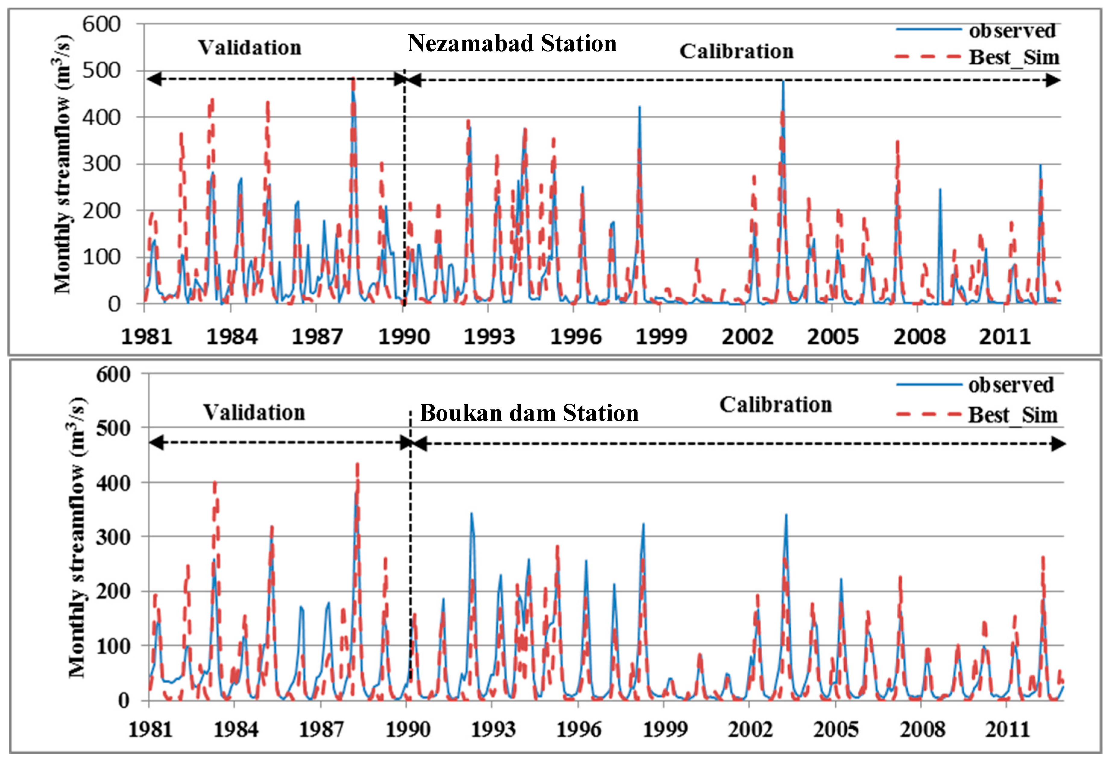
Using the SUFI-2 algorithm of SWAT-CUP, the SWAT-model was calibrated on the ZRB streamflow for the 1991–2012 and validated for the 1981–1990 period. To that avail, the 11 most sensitive parameters (the non-starred parameters in Table 2) were optimized for the eight groups of sub-basins from the upstream outlets (sub-basin 9, 10, 11) to the main outlet of the basin (subbasin 2) starting with some initial ranges, which are based on previous studies [15,23] and the knowledge of the basin. The minimum and maximum allowable value of each parameter is also considered in the calibration and validation procedures based on the SWAT model documentation [37]. Then, several iterations with about 500 simulations each were performed to determine the distribution and the 95%- prediction uncertainty of the misfit (observed-modeled streamflow) objective function.
For the validating the calibrated SWAT model, the first four years of the available data (1977–1981) are used for the warm-up of the model and the final value or range of the parameters calculated in the calibration procedure, are applied in the SWAT model and the performance indices of the results are evaluated for the next 10 years. It should be also noted that the first 10 years are selected for the validation in order to balance the dry-wet years of the calibration and validation period, as Arnold et al. [38] suggested that both wet and dry periods should be included in both the calibration and validation periods.
The statistical results of the optimized objective (misfit) functions for the six sub-basins’ outlet stations of Figure 3a are listed in terms of R2, NS and the bR2 in Table 3 for the calibration- and the validation period. Based on these numbers, particularly bR2 as the most important parameter highlighted in bold in Table 3, the fit of the model to the data (streamflow) can be considered as quite satisfactory based on the literature [21,39] for both the calibration and the validation period. The final value/range obtained for the adjusted calibration parameters is given in Table 2, wherefore the range reflects the values obtained for the eight different groups of sub-basins, and calibration parameters, superscribed by (*), denote a constant value determined for the whole basin.
The good SWAT-model performance can also be seen from Figure 4, which shows observed and simulated monthly hydrographs for outflow station 8 measuring the inflow to the Boukan reservoir dam and the outflow station 2 as the main outlet of the basin which is marked with a red circle in Figure 3a. However, some peaks are underestimated because of the occurrence of the some dry years with low precipitation, especially, during 1998–2002.
4.3. SDSM- Downscaling of CanESM2- Historical Temperatures
Based on a cross-correlation analysis of the CanESM2- temperature predictors with the observed historical daily temperatures, the three highest correlating predictors, ncep_mslp (mean sea level pressure), ncep_shum (near surface specific humidity) and ncep_temp (mean temperature at 2 m) were selected in the SDSM-regression model for the downscaled prediction of the min. temperature, whereas the two predictors ncep_p500 (500 hPa geopotential height) and ncep_temp were employed for the max. temperature.
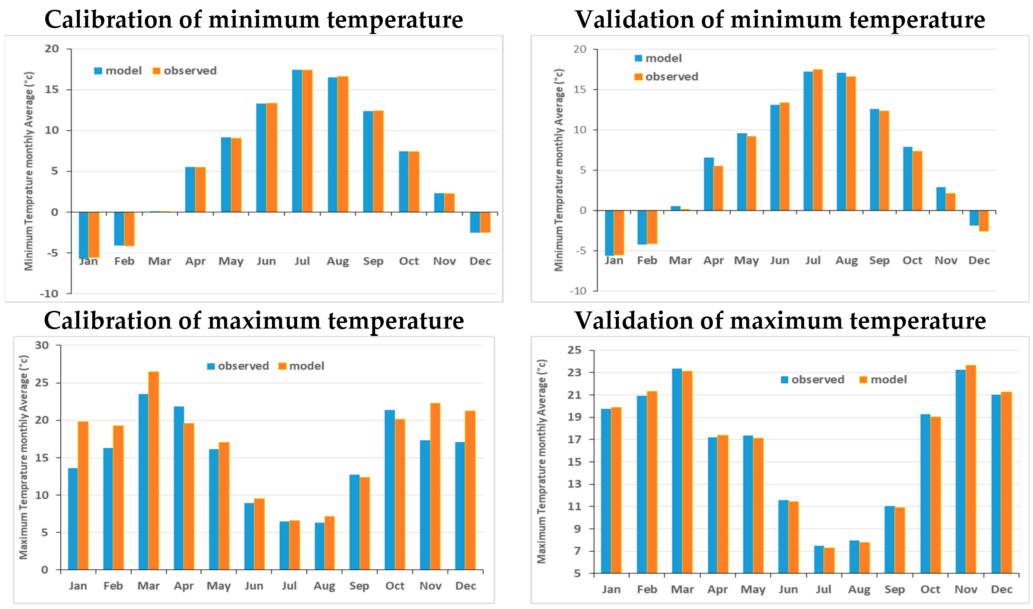
Table 4 and Figure 5 show the statistical results of SDSM- downscaled predictions of these two temperature predictands after monthly aggregation for both the calibration (1977–1998) and the validation (1999–2005) period at the CRU grid points. One can notice a very good agreement between observed and downscaled monthly variables, though this holds somewhat less for the min. temperature in the validation period. This visual impression is also corroborated by the rather high, respective, low values for the coefficient of determination (R2) and the standard error (SE) of the calibrated and validated model listed in Table 4.
It should be noted that the ECDF- QM method was also tested with temperature predictors from the MPI-ESM-LR GCM model but turned out lower model performance than SDSM in the validation period (R2 = 0.38 and SE = 6.85 against R2 = 0.73 and SE = 1.81). This is the reason for using SDSM for temperature downscaling above.
4.4. QM-Downscaling of MPI-ESM-LR Precipitation Predictors
For the validation of the two QM-downscaling variants employed, i.e., ECDF and the KDF, procedures, 10 series realizations of cross validation were carried out for 20 years, randomly selected between years 1977 and 2005, and then evaluated using the quantile bias (QBt) parameter for different percentiles t on the monthly aggregated data (see Equation (6)). Table 4 shows the results obtained for the two QM-variants. One may notice that while the raw GCM (MPI-ESM-LR)- predicted precipitation mostly overestimates the observed one (QBt > 1), - with the exception of the more extreme 75% percentile, where GCMs are usually known to underestimate the real precipitation - KDF- and ECDF-bias corrected precipitation underestimate it slightly (QBt < 1). However, with the ECDF-QBt values closer to 1, i.e., this QM-variant works better than the other one. Based on these results, only the ECDF-QM-variant is further applied in the subsequent analysis.
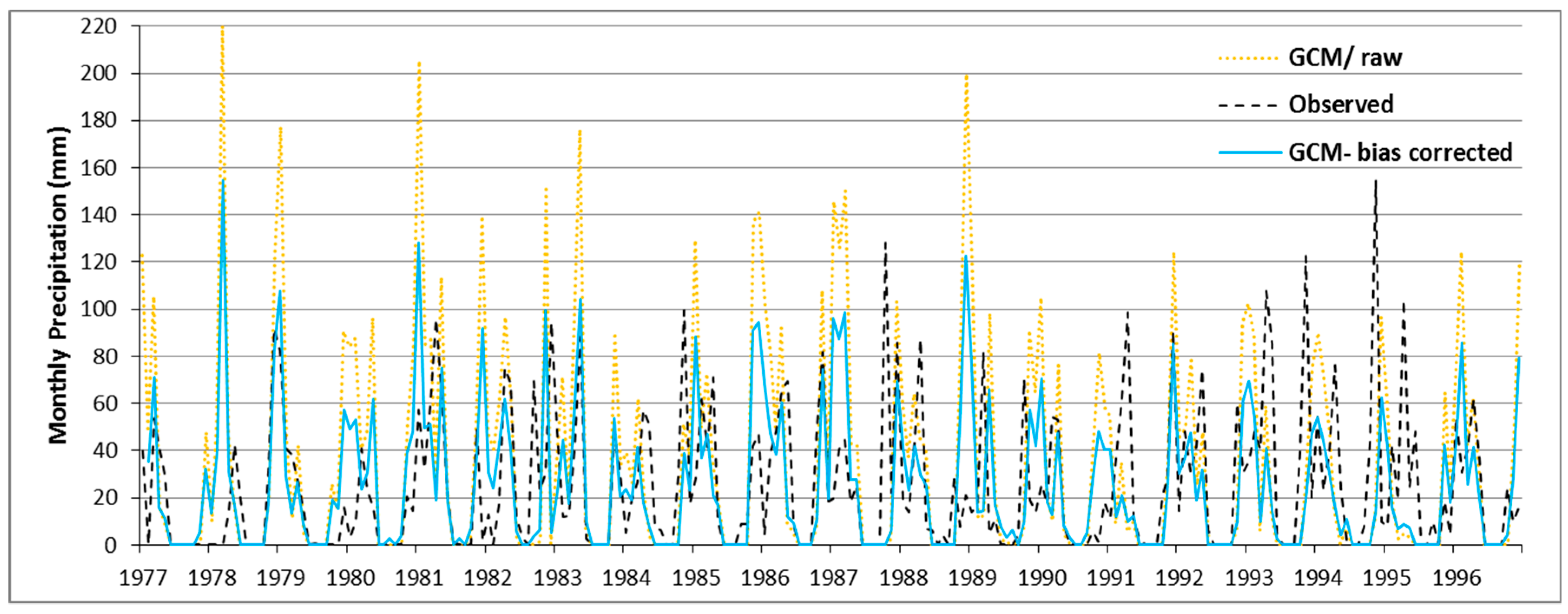
The effects of the ECDF-QM application on the historical precipitation are shown at the meteorological station Nouroozloo as an example in Figure 6. Corroborating the results of Table 5, one may notice that while the raw GCM precipitation overestimates the observed one, the ECDF – biased corrected comes much closer to the latter. Similarly good results (0.75 < QBt < 1) are obtained for other stations, but not shown here.
Using the underlying procedures of the ECDF-QM method, as epitomized by Equations (2)–(5), the future monthly MPI-ESM-LR- precipitation- predictors under radiation forcing scenarios RCP 2.6, RCP 4.5 and RCP 8.5 for years 2006 to 2029 were bias-corrected. Figure 7 shows the empirical CDFs of the observed, raw historic GCM, raw future GCM of the RCP 4.5 scenario and the bias-corrected future GCM precipitation for months of March and December at the Nouroozloo precipitation gauging station. Again, the previously mentioned overestimation of the historic precipitation by the raw GCM-predictions is clearly noticeable which leads to a corresponding “downward” correction of the future raw GCM- predictions. Similar results were obtained for other stations and other months and are not presented here.
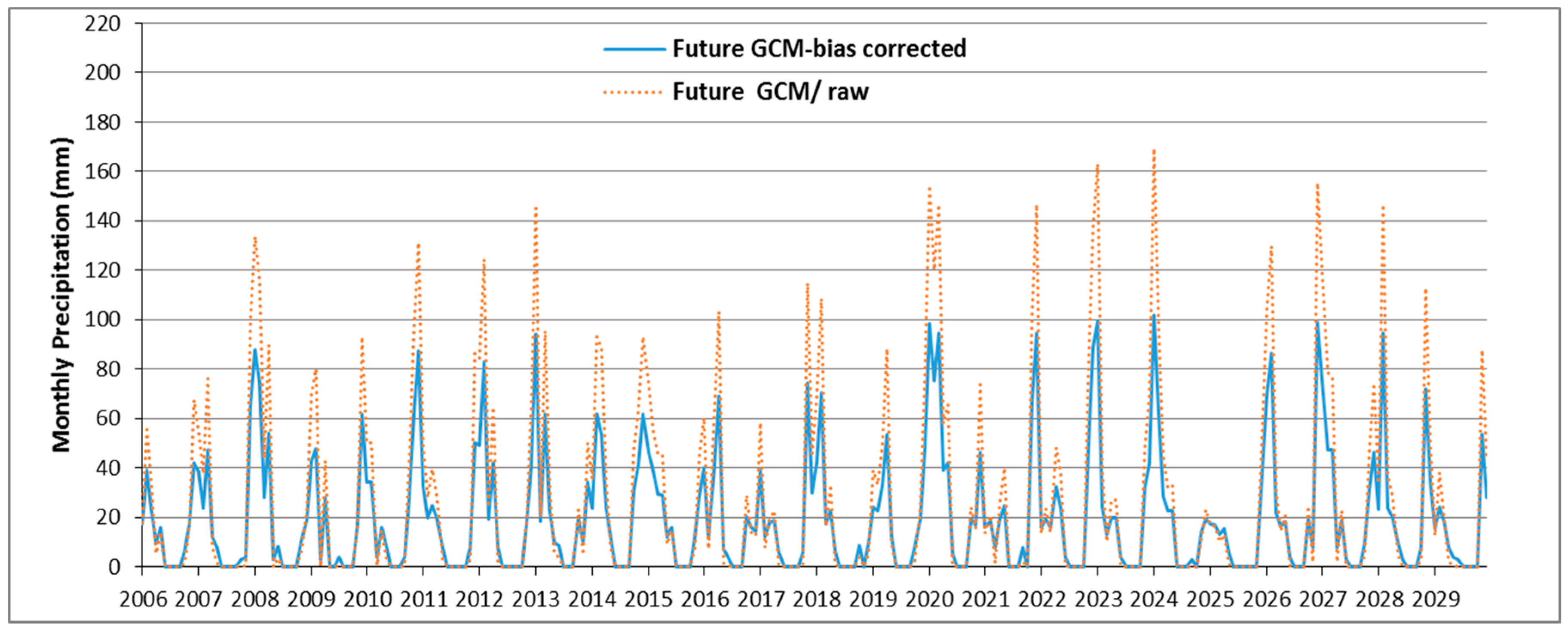
Finally daily precipitation values were generated from the monthly biased corrected data for the two RCP -scenarios by means of the stochastic Markov-chain approach for the sequence of wet and dry days in a month and random drawing from the appropriate ECDF and scaling to get the correct precipitation amount (see Section 3.2.2). With this procedure, 10 stochastic realizations of future daily precipitation were generated which will be further processed for use as input in the SWAT- model in the subsequent section. Figure 8 shows the future (2006–2029) bias-corrected monthly precipitation series generated from the average of these realizations, together with the raw future GCM- precipitation, for scenario RCP 2.6 for station Nouroozloo. In agreement with Figure 7, the QM- bias corrected monthly precipitation is consistently lower than the raw GCM-data.
4.5. SWAT Future Dam Inflow Simulations for Various Climate Scenarios
For the simulation of future streamflow in the ZRB and, particularly, of the inflow to the Boukan Dam, three possible representative future precipitation series for each RCP scenario, RCP 2.6, 4.5 and 8.5, called hitherto PA, PB and PC, were selected from the aforementioned realization-set of 10 QM- stochastically generated daily precipitation series. The PA- scenario has the less predicted rainy days, the PC- scenario the most, and the PB- scenario represent the 10-realizations average.
The precipitations predicted in this way for the three RCP-scenarios (2.6, 4.5 and 8.5) were then inputted as drivers into the previously calibrated SWAT- model, together with the downscaled min. and max. temperature for three RCP 2.6, 4.5 and 8.5- (named here TA, TB and TC, respectively), resulting in a total of nine possible climate scenarios, to predict the future reservoir dam inflow.
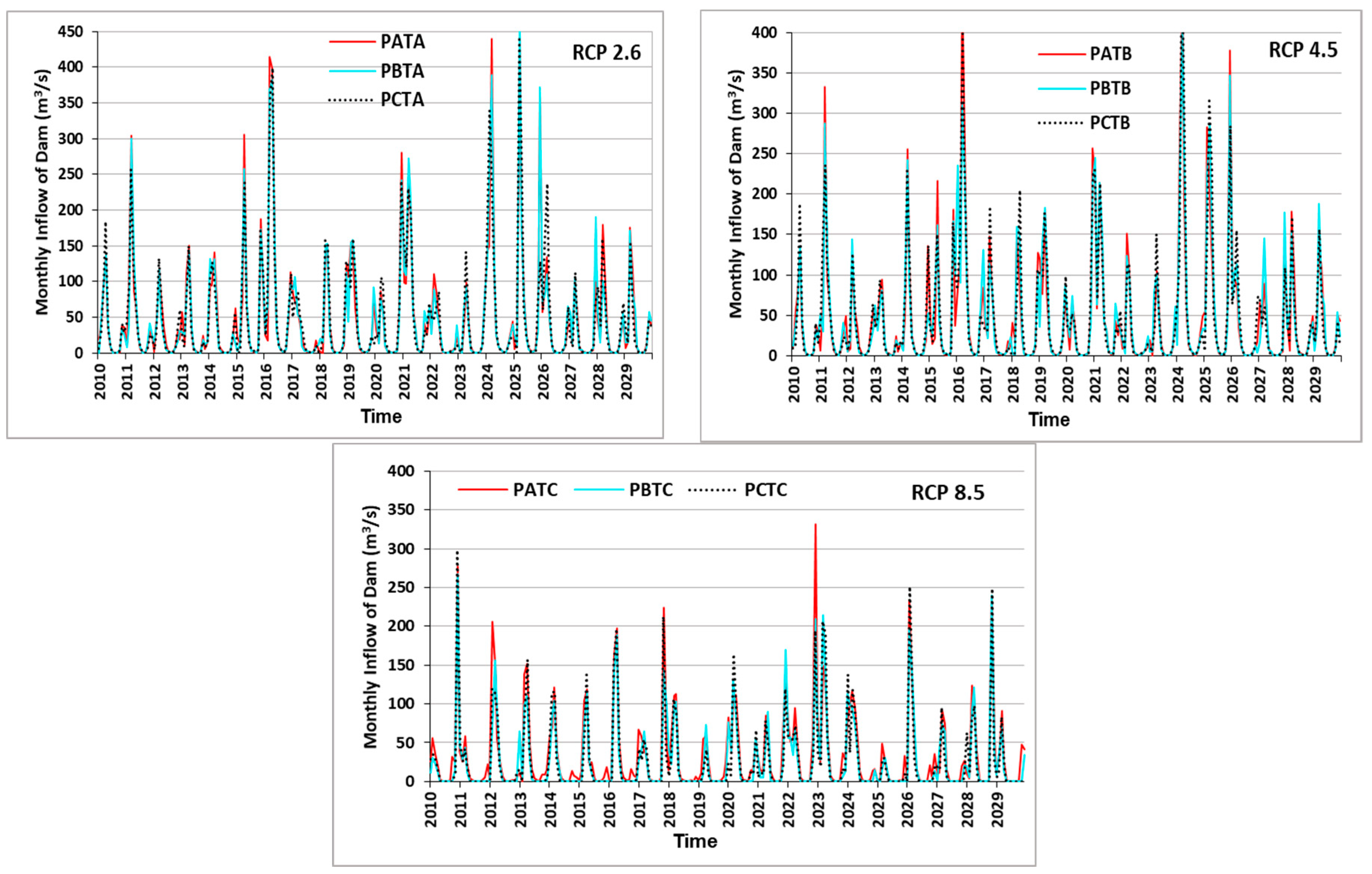
Figure 9 shows the SWAT-simulated future inflow variations to the Boukan Dam for these nine climate scenarios. Comparing the future streamflows predicted for the different scenarios, one may recognize that the trends are more or less the same, though different extreme values may arise. In general, the future predicted inflows are larger for RCP 4.5 (top right panels) for RCP 2.6 (top left panel) than the more extreme RCP 8.5 (bottom panel), while the highest streamflow are predicted for the lowest emission scenario, RCP 2.6 (top left panel) as expected.
The same holds for the responses to the three temperature scenarios where the inflows are larger for the mild RCP 2.6- and RCP 4.5- than the more extreme RCP 8.5- scenario. On the other hand, within each RCP-group, the inflows are approximately the same for the three assumed future precipitation realizations, PA, PB and PC.
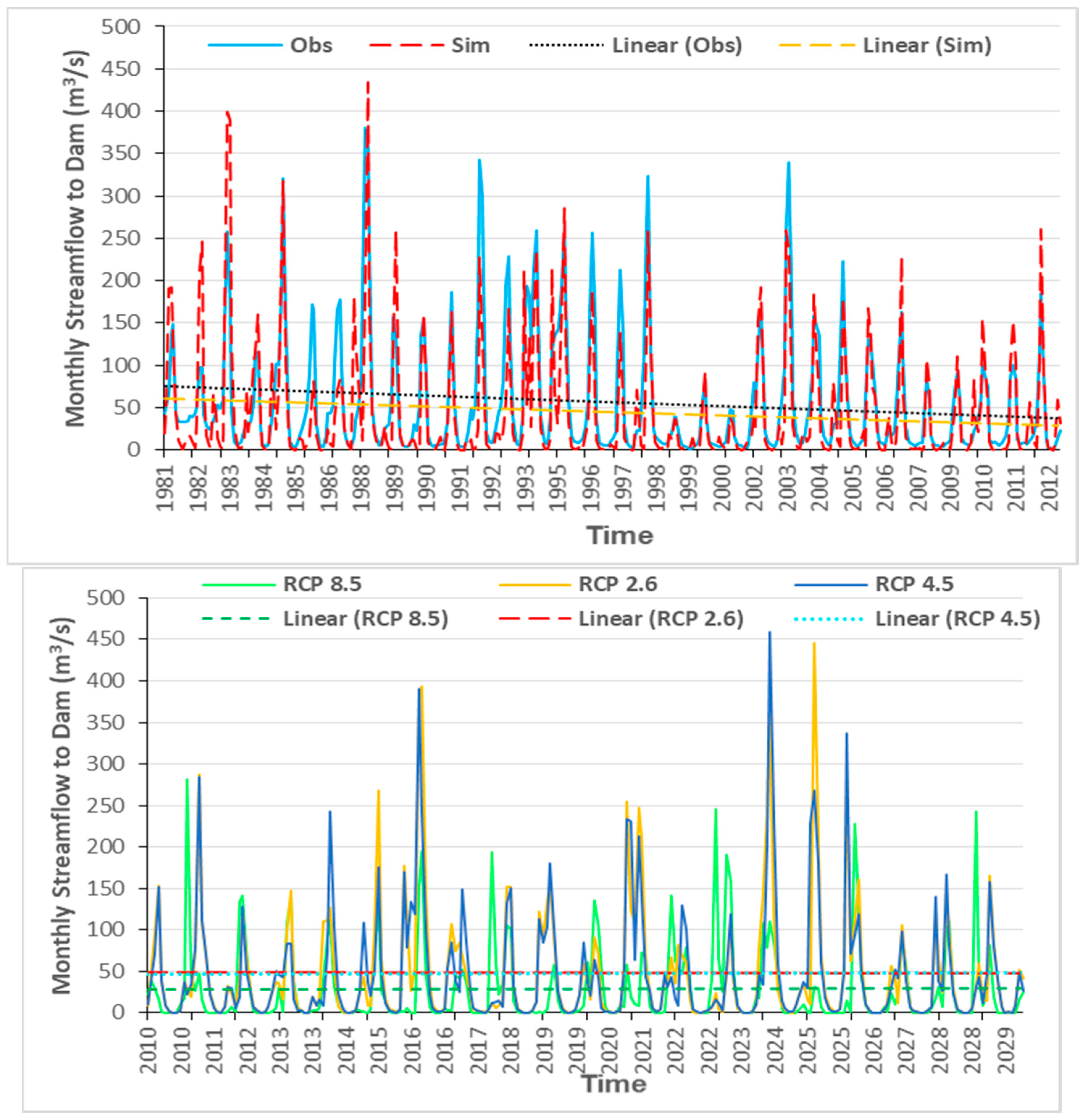
While the predicted Boukan Dam inflow differences for the nine climate scenarios appear to be only minor, particularly for the medium scenarios (RCP 2.6 and 4.5), this is not the case when comparing the future dam inflow with the historical one, as illustrated in Figure 10 for the average of the three variants for each of the three RCP-scenarios. This figure shows that, compared with the historical streamflow of the late 20th century, of the 2006–2029 time period has decreased remarkably; meanwhile, the decreasing trend in the observed period will be changed to a constant trend in the future period. The RCP 2.6 and 4.5 trends are almost the same and the lowest average of inflow is for the RCP 8.5.
The above predicted changes of the future inflow to the Boukan Dam, the major water supply reservoir in the ZRB, will have significant adverse implications on the water supply in the basin, requiring various adaptation strategies, especially, for agriculture, such as reduced or more efficient irrigation, or even changing the crop patterns, as has been indicated by e.g., Emami and Koch [40] for this agriculturally used basin in Iran.
The various water balance parameters for the whole ZRB, which are either input to SWAT (precipitation) or simulated, are presented in Table 6 as averages of the six variants for each of the two climatic scenarios, RCP 2.6 and RCP 4.5, together with those obtained for the historical reference period. One will notice from the table that, in comparison with the validation period (1981 to 1990), precipitation (rainfall plus snowfall) will decrease gradually by 17%, 20% and 30% for the three RCPs, respectively. For the snowmelt, the reductions are with 18%, 26% and 38% even more tremendous. Relative to the later calibration period (1991 to 2012), the reduction of future precipitation will be about 11%, 11% and 9% less for the RCPs, while snowmelt will be 20%, 18% and 15% less for RCP 2.6 and 4.5 scenarios, respectively. The decreasing average of snowfall and sublimation also agrees with the reducing trend of snowmelt in the predicted scenarios.
Evapotranspiration (ET) shows also a decreasing trend in the future years, with the latter being, somewhat expectedly, stronger for RCP 8.5 than for RCP 4.5 and for RCP 4.5 than for RCP 2.6, whereas the shallow aquifer recharge is also reduced for all RCPs, though somewhat less for RCP 2.6 and RCP 4.5, respectively.
The future declining trends in the above mentioned parameters will have direct consequences on the three important routing contributors, surface runoff (SWQ), lateral subsurface flow (LWQ) and groundwater inflow (GWQ) which make up (minus the transmission losses, TLOSS) the streamflow in the main channel, i.e., the water yield WYLD, as framed by the red line in Table 6. Thus, when compared with the historical period, these three flow components will be significantly lower in the future for the two RCP scenarios and, with it, the total water yield, which decreases by 17%, 30% and 39% for RCP 2.6, 4.5 and 8.5, respectively. In fact, this reduction is mostly due to the large drop of the groundwater contribution (GWQ) to the main stream, which is by 25% to 46%, on average.
The ratio of the surface runoff SWQ to the liquid precipitation plus snowmelt defines the surface runoff coefficient RC [41]. It is predicted to have on average a slight increase which is more for RCP 4.5 (from 15% and 12% in validation and calibration periods to 17%, 16% and 15% in RCP 2.6, RCP 4.5 and RCP 8.5, respectively), as the liquid precipitation plus the snowmelt (denominator of the RC-ratio) will have a stronger reduction by 22% to 34% than the average surface runoff with only a 2%, 10% and 26% decrease for RCP 2.6, RCP 4.5 and RCP 8.5, respectively. Based on the values in Table 5, one may also notice that, despite the fact that the surface runoff and, consequently, the inflows to the Boukan Dam will decline by 18%, 24% and 38% for the three RCPs, respectively, compared to the validation period 1981–1990, but increase by 20% and 11% and decrease by 9% in comparison with the later calibration period 1991–2012 for the three RCPs, because of the decreasing evapotranspiration and losses.
In summary, the impacts of climate change on the water balance of the ZRB will overall be negative, as the available freshwater resources will be diminished for the three future climate scenarios investigated. Based on these predictions, there is a higher likelihood of a future water scarcity in the ZRB, unless some adaptation strategies are implemented, e.g., construction of new hydraulic storage facilities and/or changing agricultural crop pattern that are more prone to resist water scarcity.
5. Conclusions
The impacts of a changing climate on inflows in the Boukan Dam and on general water availability in the Zarrine river basin (ZRB) were investigated, using the basin-wide SWAT- hydrologic model, driven by GCM- climate predictors, downscaled by the statistical downscaling method (temperatures), and a nonstationary CDF-matching Quantile Mapping (QM)- bias correction technique (precipitation) for different climate scenarios (RCPs)sd.
SWAT was first calibrated and validated satisfactorily for six available discharge stations around the basin, one by one, for the historical reference period 1981–2012 and then used to predict future hydrological basin parameters, namely, streamflow (water yield) up to year 2029. Input precipitation to the model is based on an MPI-ESM-LR model from CMIP5 GCM simulation results for RCP 2.6, RCP 4.5 and RCP 8.5 scenarios, downscaled by QM with two variants, Kernel Density Function and Empirical CDF (ECDF). Owing to the better performance of the latter, the QM-ECDF variant was applied to the raw GCM-precipitation in the study area and turned out to be able to significantly reduce the biases of the latter. Input minimum and maximum temperatures to the SWAT- model were SDSM—(a hybrid of multiple linear regression and stochastic weather generator) downscaled predictors of the CanESM2 GCM.
To evaluate the impacts of future climate variations on water availability in the ZRB, the SWAT-predicted hydrological changes were investigated, i.e., water balance components, including the weather inputs, precipitation, snowfall and snowmelt and evaporation, and three main routing contributors, surface water, lateral flow and groundwater to the water yield as the net available water resources in the basin are compared for the historic (reference) and future periods under RCP 2.6, RCP 4.5 and RCP 8.5 climate scenarios.
The results of this analysis indicate that the impacts of future climate change on the water balance in the ZRB will generally be negative in the recent/near future period 2012–2029, as the long-term river discharge and with it the inflow of the Boukan Dam, the major water reservoir in the basin, will decrease, particularly, for RCP 8.5. This holds also for the total water yield of the watershed which will decrease by −17% (RCP 2.6), −30% (RCP 4.5), and −39% (RCP 8.5), as rainfall, lateral flow and groundwater baseflow, in particular, to the main channel diminish. Nevertheless, the future runoff coefficient shows a slight 3% (RCP 2.6), 2% (RCP 4.5) and 1% (RCP 8.5) increase, as the future precipitation decreases more (~−28%) than the surface runoff (~−12%).
Thus, considering these predicted future drops of the available water resources, together with a concurrent future increase of the water demand, due to further agricultural- and other development plans for the ZRB, the necessity of an adaptation plan to mitigate these negative impacts of climate change on the ZR-streamflow, as well as on Lake Urmia with its fragile ecosystem. The adverse situation could be further exacerbated by the possible emergence of more climate extremes, as indicated for the basin in Iran by Emami and Koch [7].
Based on the research proposed here, a case for further studies can be provided to deal with water management and decision-making on the basin scale in Iran, in order to better respond to changing future water availability with some adaptation plans. The modelling approach used in the present study could be used for a high-resolution analysis of water resources system and further as a base tool for managing available freshwater resources with a sustainable and optimal river basin management approach, such as MODSIM [42]. Moreover, as it has been shown in the present study that groundwater plays a significant role in the total water yield of the basin, a better understanding of the characteristics of the groundwater system in the basin should be obtained which could be achieved by coupling the SWAT- surface water model with a groundwater model, such as MODFLOW, as done by Izady et al. [43] in a similar basin in the region.
Author Contributions
M.K. supervised the research. F.E. conceived the research, implemented the procedures and wrote the outline of the manuscript. Both authors contributed to finalizing the manuscript, with M.K. doing the final major editing.
Funding
F.E. received funding from the Deutscher Akademischer Austauschdienst (DAAD) for carrying out his Ph.D. studies related to the topic of the present research.
Conflicts of Interest
The authors declare no conflict of interest.
References
- Water for Food, Water for Life: A Comprehensive Assessment of Water Management in Agriculture; Earthscan: London, UK; International Water Management Institute: Colombo, Sri Lanka, 2007.
- Voss, K.A.; Famiglietti, J.S.; Lo, M.; Linage, C.D.; Rodell, M.; Swenson, S.C. Groundwater depletion in the Middle East from GRACE with implications for transboundary water management in the Tigris-Euphrates-Western Iran region. Water Resour. Res. 2013, 49, 904–914. [Google Scholar] [CrossRef]
- Madani, K. Water Management in Iran: What is causing the looming crisis? J. Environ. Stud. Sci. 2014, 4, 315–328. [Google Scholar] [CrossRef]
- Punkari, M.; Droogers, P.; Immerzeel, W.; Korhonen, N.; Lutz, A.; Venäläinen, A. Climate Change and Sustainable Water Management in Central Asia; Working Paper Series No. 5; Asian Development Bank (ADB) Central and West Asia: Manila, Philippines, 2014. [Google Scholar]
- Abbaspour, K.C.; Faramarzi, M.; Ghasemi, S.S.; Yang, H. Assessing the Impact of Climate Change on Water Resources of Iran. Water Resour. Res. 2009, 45, W10434. [Google Scholar] [CrossRef]
- Blanc, E.; Strzepek, K.; Schlosser, A.; Jacoby, H.; Gueneau, A.; Fant, C.; Rausch, S.; Reilly, J. Analysis of U.S. Water Resources under Climate Change; MIT Joint Program on the Science and Policy of Global Change, Report No. 239; Massachusetts Institute of Technology: Cambridge, MA, USA, 2013. [Google Scholar]
- Emami, F.; Koch, M. Evaluation of Statistical-Downscaling/Bias-Correction Methods to Predict Hydrologic Responses to Climate Change in the Zarrine River Basin, Iran. Climate 2018, 6, 30. [Google Scholar] [CrossRef]
- Tegegne, G.; Hail, I.D.; Aranganathan, S.M. Evaluation of Operation of Lake Tana Reservoir Future Water Use under Emerging Scenario with and without climate Change Impacts, Upper Blue Nile. Int. J. Comput. Technol. 2013, 4, 654–663. [Google Scholar] [CrossRef]
- Ashraf Vaghefi, S.; Mousavi, S.J.; Abbaspour, K.C.; Srinivasan, R.; Yang, H. Analyses of the impact of climate change on water resources components, drought and wheat yield in semiarid regions: Karkheh River Basin in Iran. Hydrol. Process. 2014, 2018–2032. [Google Scholar] [CrossRef]
- Pengra, B. The Drying of Iran’s Lake Urmia and Its Environmental Consequences; UNEP-GRID; UNEP Global Environmental Alert Service (GEAS): Sioux Falls, SD, USA, 2012. [Google Scholar]
- AghaKouchak, A.; Norouzi, H.; Madani, K.; Mirchi, A.; Azarderakhsh, M.; Nazemi, A.; Nasrollahi, N.; Farahmand, A.; Mehran, A.; Hasanzadeh, E. Aral Sea syndrome desiccates Lake Urmia: Call for action. J. Great Lakes Res. 2015, 41, 307–311. [Google Scholar] [CrossRef]
- Neitsch, S.L.; Arnold, J.G.; Kiniry, J.R.; Williams, J.R. Soil and Water Assessment Tool Theoretical Documentation Version 2009; Texas Water Resources Institute: Temple, TX, USA, 2011. [Google Scholar]
- Jha, M.; Pan, Z.; Takle, E.S.; Gu, R. Impacts of climate change on streamflow in the Upper Mississippi River Basin: A regional climate model perspective. J. Geophys. Res. 2004, 109, D09105. [Google Scholar] [CrossRef]
- Iranian Ministry of Jahade-Agriculture (MOJA). Land Cover Classification; Agricultural Statistics and the Information Center: Tehran, Iran, 2007.
- Ahmadzadeh, H.; Morid, S.; Delavar, M.; Srinivasan, R. Using the SWAT model to assess the impacts of changing irrigation from surface to pressurized systems on water productivity and water saving in the Zarrineh Rud catchment. Agric.Water Manag. 2015. [Google Scholar] [CrossRef]
- Abbaspour, K.C.; Johnson, C.A.; van Genuchten, M.T. Estimating uncertain flow and transport parameters using a sequential uncertainty fitting procedure. J. Vadose Zone 2004, 3, 1340–1352. [Google Scholar] [CrossRef]
- Abbaspour, K.C. SWAT-Calibration and Uncertainty Programs (CUP)—A User Manual; Swiss Federal Institute of Aquatic Science and Technology: Eawag, Duebendorf, 2015. [Google Scholar]
- Koch, M.; Cherie, N. SWAT-Modeling of the Impact of future Climate Change on the Hydrology and the Water Resources in the Upper Blue Nile River Basin, Ethiopia. In Proceedings of the 6th International Conference on Water Resources and Environment Research, ICWRER, Koblenz, Germany, 3–7 June 2013. [Google Scholar]
- Van Griensven, A.; Meixner, T. Dealing with unidentifiable sources of uncertainty within environmental models. In Proceedings of the International Environmental Modelling and Software Society Conference, Osnabrück, Germany, 15–19 June 2014. [Google Scholar]
- Gassman, P.W.; Reyes, M.R.; Green, C.H.; Arnold, J.G. The soil and water assessment tool: Historical development, applications, and future research directions. Trans. ASABE 2007, 50, 1211–1250. [Google Scholar] [CrossRef]
- Krause, P.; Boyle, D.P.; Base, F. Comparison of different efficiency criteria for hydrological model assessment. Adv. Geosci. 2005, 5, 89–97. [Google Scholar] [CrossRef]
- Themeßl, M.J.; Gobiet, A.; Leuprecht, A. Empirical-statistical downscaling and error correction of daily precipitation from regional climate models. Int. J. Climatol. 2011, 31, 1530–1544. [Google Scholar] [CrossRef]
- Emami, F. Development of an algorithm for assessing the impacts of climate change on operation of reservoirs. Master’s Thesis, University of Tehran, Tehran, Iran, 2009. [Google Scholar]
- Sarzaeim, P.; Bozorg-Haddad, O.; Fallah-Mehdipour, E.; Loáiciga, H.A. Climate change outlook for water resources management in a semiarid river basin: The effect of the environmental water demand. Environ. Earth Sci. 2017, 76, 498. [Google Scholar] [CrossRef]
- Van Vuuren, D.P.; Edmonds, J.; Kainuma, M.L.T.; Riahi, K.; Thomson, A.; Matsui, T.; Hurtt, G.; Lamarque, J.F.; Meinshausen, M.; Smith, S.; et al. Representative concentration pathways: An overview. Clim. Chang. 2011, 109. [Google Scholar] [CrossRef]
- Wilby, R.L.; Dawson, C.W.; Barrow, E.M. SDSM—A decision support tool for the assessment of regional climate change impacts. Environ. Model. Softw. 2002, 17, 147–159. [Google Scholar] [CrossRef]
- Wilby, R.L.; Dawson, C.W. Statistical Downscaling Model–Decision Centric (SDSM-DC) Version 5.1 Supplementary Note; Loughborough University: Loughborough, UK, 2013. [Google Scholar]
- Hessami, M.; Gachon, P.; Ouarda, T.B.M.J.; St-Hilaire, A. Automated regression-based statistical downscaling tool. Environ. Model. Softw. 2008, 23, 813–834. [Google Scholar] [CrossRef]
- Themeßl, M.J.; Gobiet, A.; Heinrich, G. Empirical-statistical downscaling and error correction of regional climate models and its impact on the climate change signal. Clim. Chang. 2012, 112, 449–468. [Google Scholar] [CrossRef]
- Miao, C.; Su, L.; Sun, Q.; Duan, Q. A nonstationary bias-correction technique to remove bias in GCM simulations. J. Geophys. Res. Atmos. 2016, 121, 5718–5735. [Google Scholar] [CrossRef]
- Piani, C.; Haerter, J.O.; Coppola, E. Statistical bias correction for daily precipitation in regional climate models over Europe. Theor. Appl. Climatol. 2010, 99, 187–192. [Google Scholar] [CrossRef]
- Li, H.B.; Sheffield, J.; Wood, E.F. Bias correction of monthly precipitation and temperature fields from Intergovernmental Panel on Climate Change AR4 models using equidistant quantile matching. J. Geophys. Res. 2010, 115, D10101. [Google Scholar] [CrossRef]
- Milly, P.C.D.; Betancourt, J.; Falkenmark, M.; Hirsch, R.M.; Kundzewicz, Z.W.; Lettenmaier, D.P.; Stouffer, R.J. Climate change—Stationarity is dead: Whither water management? Science 2008, 319, 573–574. [Google Scholar] [CrossRef]
- Mehran, A.; AghaKouchak, A.; Phillips, T. Evaluation of CMIP5 continental precipitation simulations relative to satellite observations. J. Geophys. Res. Atmos. 2014, 119, 1695–1707. [Google Scholar] [CrossRef]
- Wilks, D.S. Statistical Methods in Atmospheric Sciences, 2nd ed.; Academic Press: Cambridge, MA, USA, 2006. [Google Scholar]
- Mhanna, M.; Bauwens, W. Stochastic single-site generation of daily and monthly rainfall in the Middle East. Meteorol. Appl. 2012, 19, 111–117. [Google Scholar] [CrossRef]
- Arnold, J.G.; Kiniry, J.R.; Sirinivasan, R.; Williams, J.R.; Haney, E.B.; Neitsh, S.L. SWAT Input–Output Documentation, Version 2012; Texas Water Resource Institute: College Station, TX, USA, 2012. [Google Scholar]
- Arnold, J.G.; Moriasi, D.N.; Gassman, P.W.; Abbaspour, K.C.; White, M.J.; Srinivasan, R.; Santhi, C.; Harmel, R.D.; Van Griensven, A.; Van Liew, M.W.; et al. SWAT: Model use, calibration, and validation. Trans. ASABE 2012, 55, 1491–1508. [Google Scholar] [CrossRef]
- Moriasi, D.N.; Arnold, J.G.; Van Liew, M.W.; Bingner, R.L.; Harmel, R.D.; Veith, T.L. Model evaluation guidelines for systematic quantification of accuracy in watershed simulations. Trans. ASABE 2007, 50, 885–900. [Google Scholar] [CrossRef]
- Emami, F.; Koch, M. Agricultural water productivity-based hydro-economic modeling for optimal crop pattern and water resources planning in the zarrine river basin, Iran, in the wake of climate change. Sustainability 2018, 10, 3953. [Google Scholar] [CrossRef]
- Merz, R.; Blöschl, G. A regional analysis of event runoff coefficients with respect to climate and catchment characteristics in Austria. Water Resour. Res. 2009, 45, W01405. [Google Scholar] [CrossRef]
- Emami, F.; Koch, M. Evaluating the water resources and operation of the boukan dam in iran under climate change. Eur. Water 2017, 59, 17–24. [Google Scholar]
- Izady, A.; Davary, K.; Alizadeh, A.; Ziaei, A.N.; Akhavan, S.; Alipoor, A.; Joodavi, A.; Brusseau, M.L. Groundwater conceptualization and modeling using distributed SWAT-based recharge for the semi-arid agricultural Neishaboor plain, Iran. Hydrogeol. J. 2015, 23, 47–68. [Google Scholar] [CrossRef]
Figure 1.
Flowchart of the Zarrine River Basin (ZRB)- water resources simulation study.

Figure 2.
Map of the Lake Urmia basin (Iran) with the ZRB as the major sub-basin and further delineation of the sub-basins with gauge station outlets (a) together with DEM (b); and land use cover of the ZRB (c).
Figure 2.
Map of the Lake Urmia basin (Iran) with the ZRB as the major sub-basin and further delineation of the sub-basins with gauge station outlets (a) together with DEM (b); and land use cover of the ZRB (c).

Figure 3.
(a) map of selected weather and hydrometric stations in the ZRB-SWAT model (precipitation (PCP) and temperature (TMP); (b) selected GCM- points and -gridbox of MPI-ESM-LR.
Figure 3.
(a) map of selected weather and hydrometric stations in the ZRB-SWAT model (precipitation (PCP) and temperature (TMP); (b) selected GCM- points and -gridbox of MPI-ESM-LR.

Figure 4.
Observed (solid line) and simulated (dashed line) hydrographs for outlet station 8 measuring inflow to the Boukan Dam (bottom panel) and the main basin outlet station 2, Nezamabad (top panel).
Figure 4.
Observed (solid line) and simulated (dashed line) hydrographs for outlet station 8 measuring inflow to the Boukan Dam (bottom panel) and the main basin outlet station 2, Nezamabad (top panel).

Figure 5.
Observed and simulated min. (upper panels) and max. (lower panels) monthly temperatures for calibration (left panels) and validation (right panels) periods at 452255t station.
Figure 5.
Observed and simulated min. (upper panels) and max. (lower panels) monthly temperatures for calibration (left panels) and validation (right panels) periods at 452255t station.

Figure 6.
Monthly observed and QM-downscaled (bias–corrected with ECDF and KDF) precipitation at Nouroozloo station for the calibration period 1977 to 1996.
Figure 6.
Monthly observed and QM-downscaled (bias–corrected with ECDF and KDF) precipitation at Nouroozloo station for the calibration period 1977 to 1996.

Figure 7.
Empirical CDF for daily precipitation for reference raw GCM (1977–2005), future raw GCM for the RCP4.5 scenario (2006–2029) and QM- bias-corrected data at Nouroozloo station for March and December.
Figure 7.
Empirical CDF for daily precipitation for reference raw GCM (1977–2005), future raw GCM for the RCP4.5 scenario (2006–2029) and QM- bias-corrected data at Nouroozloo station for March and December.

Figure 8.
Future (2006–2029) raw GCM- and bias corrected monthly precipitation series for scenario RCP2.6 for Nouroozloo station.
Figure 8.
Future (2006–2029) raw GCM- and bias corrected monthly precipitation series for scenario RCP2.6 for Nouroozloo station.

Figure 9.
SWAT-simulated future monthly inflows at Boukan Dam for nine climatic scenarios, i.e., RCP 2.6 (top left panel), RCP 4.5 (top right panel) and RCP 8.5 (bottom panel) for precipitation (PA, PB, PC, see text for details) and temperature (TA, TB, TC, see text for details).
Figure 9.
SWAT-simulated future monthly inflows at Boukan Dam for nine climatic scenarios, i.e., RCP 2.6 (top left panel), RCP 4.5 (top right panel) and RCP 8.5 (bottom panel) for precipitation (PA, PB, PC, see text for details) and temperature (TA, TB, TC, see text for details).

Figure 10.
Monthly observed (historical), simulated (historical) together with trend lines for the historical (top panel) and future predicted (bottom panel) inflow into the Boukan Dam based on average of RCP 2.6, RCP 4.5 and RCP 8.5 climatic scenarios (see text), together with trend lines for historical and future predicted periods.


Table 1.
Ranks of the most sensitive l parameters of the basin with their final calibrated values.
| Rank | Parameter | Final Value | Rank | Parameter | Final Value |
|---|---|---|---|---|---|
| 1 | SFTMP.bsn | 1 | 5 | SMFMX.bsn | 7.95 |
| 2 | SMTMP.bsn | 0.5 | 6 | SMFMN.bsn | 0.73 |
| 3 | SNO50COV.bsn | 0.3 | 7 | SNOCOVMX.bsn | 463.9 |
| 4 | TIMP.bsn | 0.71 |
Table 2.
Ranked most sensitive SWAT-parameters with final calibrated range for the different sub-basins.
Table 2.
Ranked most sensitive SWAT-parameters with final calibrated range for the different sub-basins.
| Rank | Parameter | Dimension | Final Range | Rank | Parameter | Dimension | Final Range |
|---|---|---|---|---|---|---|---|
| 1 | CN2.mgt | dimensionless | 35–89 | 9 | SOL_AWC(1).sol | mm H2O/mm | 0.09–0.34 |
| 2 | SOL_BD(1).sol | g/cm3 | 0.9–1.96 | 10 | ALPHA_BF.gw | 1/day | 0.25–0.96 |
| 3 | SOL_Z(1).sol | mm | 132–476 | 11 | REVAPMN.gw | mm H2O | 162–407 |
| 4 | ALPHA_BNK.rte | days | 0.27–0.65 | 12 | GW_SPYLD.gw * | m3/m3 | 0.05 |
| 5 | GWQMN.gw | mm H2O | 1076–3827 | 13 | CH_K2.rte * | mm/h | 0.5 |
| 6 | ESCO.hru | dimensionless | 0.91–0.99 | 14 | RCHRG_DP.gw * | dimensionless | 0 |
| 7 | SOL_K(1).sol | mm/h | 4–22 | 15 | CH_N2.rte * | dimensionless | 0.016 |
| 8 | GW_DELAY.gw | day | 10–35 |
* Final value of these parameters applies to the whole basin.
Table 3.
Statistical measures for the SUFI-2-optimized objective functions for calibration and validation periods for various sub-basin outlet stations together with uncertainty measures (P- and R-factor).
Table 3.
Statistical measures for the SUFI-2-optimized objective functions for calibration and validation periods for various sub-basin outlet stations together with uncertainty measures (P- and R-factor).
| Sub-Basin Outlet | Station | Calibration | Validation | ||||||||
|---|---|---|---|---|---|---|---|---|---|---|---|
| P-f * | R-f * | R2 | NS | bR2 | P-f * | R-f * | R2 | NS | bR2 | ||
| 2 | Nezamabad | 0.90 | 1.1 | 0.72 | 0.65 | 0.66 | 0.8 | 1.4 | 0.57 | 0.51 | 0.50 |
| 4 | Chooblooche | 0.82 | 1.0 | .060 | 0.30 | 0.60 | 0.9 | 1.1 | 0.66 | 0.55 | 0.56 |
| 7 | Sarighamish | 0.92 | 1.2 | 0.68 | 0.55 | 0.67 | 0.7 | 1.4 | 0.63 | 0.45 | 0.52 |
| 8 | Boukan Dam | 0.79 | 1.4 | 0.76 | 0.72 | 0.58 | 0.8 | 1.4 | 0.60 | 0.50 | 0.54 |
| 9 | Safakhaneh | 0.85 | 1.1 | 0.66 | 0.40 | 0.62 | 0.8 | 1.2 | 0.59 | 0.45 | 0.55 |
| 11 | Sonateh | 0.86 | 1.1 | 0.64 | 0.42 | 0.63 | 0.6 | 1.7 | 0.55 | 0.44 | 0.30 |
| Average | 0.86 | 1.2 | 0.68 | 0.51 | 0.63 | 0.8 | 1.4 | 0.60 | 0.48 | 0.50 | |
* P-f and R-f stands for P-factor and R-factor of the model, respectively.
Table 4.
R2 and SE of SDSM- downscaled monthly temperatures for calibration and validation periods.
| Parameter | Station Name | R2 | SE | ||
|---|---|---|---|---|---|
| Calibration | Validation | Calibration | Validation | ||
| Min. Temperature | 452255t | 0.66 | 0.74 | 2.03 | 1.65 |
| 453253t | 0.59 | 0.65 | 2.40 | 2.07 | |
| 453254t | 0.63 | 0.69 | 2.18 | 1.78 | |
| 454252t | 0.57 | 0.58 | 2.44 | 2.11 | |
| 454254t | 0.61 | 0.72 | 2.12 | 1.55 | |
| 454255t | 0.65 | 0.76 | 2.03 | 1.60 | |
| 455253t | 0.60 | 0.68 | 2.31 | 1.79 | |
| Max. Temperature | 452255t | 0.71 | 0.79 | 2.01 | 1.81 |
| 453253t | 0.75 | 0.71 | 1.76 | 2.11 | |
| 453254t | 0.73 | 0.81 | 2.05 | 1.65 | |
| 454252t | 0.69 | 0.78 | 2.22 | 1.76 | |
| 454254t | 0.73 | 0.79 | 2.15 | 1.79 | |
| 454255t | 0.71 | 0.79 | 2.12 | 1.80 | |
| 455253t | 0.68 | 0.77 | 2.20 | 1.81 | |
| Average | 0.67 | 0.73 | 2.14 | 1.81 | |
Table 5.
Precipitation quantile bias (QBt) as a function of the percentile obtained with the raw GCM, KDF and ECDF-QM variants.
Table 5.
Precipitation quantile bias (QBt) as a function of the percentile obtained with the raw GCM, KDF and ECDF-QM variants.
| Percentile | QBt | ||
|---|---|---|---|
| Raw GCM | KDF | ECDF | |
| 25% | 1.48 | 0.69 | 0.96 |
| 50% | 1.35 | 0.57 | 0.87 |
| 75% | 0.86 | 0.46 | 0.79 |
| Average | 1.23 | 0.57 | 0.88 |
Table 6.
Annual SWAT-modeled water balance components for the ZRB for the historical reference period (1981–2012) (validation (1981–1990), calibration (1991–2012), and average) and the averages of the six variants for each of the two climatic scenarios, RCP 2.6 and RCP 4.5 for the future period (2012–2029). Red line bordered cells mark the flow contributions to the total water yield (streamflow).
| Water Balance Components (mm/a) | Historical Period | RCP 2.6 | RCP 4.5 | RCP 8.5 | |||
|---|---|---|---|---|---|---|---|
| Validation | Calibration | Average | |||||
| Precipitation | 454.6 | 393.1 | 423.9 | 327.2 | 313 | 276 | |
| (−23%) * | (−26%) | (−35%) | |||||
| Snowfall | 145 | 118.3 | 131.7 | 92.8 | 85.6 | 71.36 | |
| (−30%) | (−35%) | (−46%) | |||||
| Sublimation | 38.5 | 38.5 | 38.5 | 32.5 | 27.8 | 24.12 | |
| (−16%) | (−28%) | (−37%) | |||||
| Snowmelt | 105.9 | 79.7 | 92.8 | 65.7 | 58.8 | 49.8 | |
| (−29%) | (−37%) | (−46%) | |||||
| Aquifer Recharge | Shallow | 174.2 | 148.4 | 161.3 | 105.1 | 99.5 | 81.84 |
| (−35%) | (−38%) | (−49%) | |||||
| Deep | 1.4 | 1.1 | 1.3 | 1.1 | 0.7 | 0.72 | |
| (−15%) | (−46%) | (−45%) | |||||
| Evapotranspiration | 254.8 | 253.5 | 254.2 | 197.5 | 209.9 | 162.96 | |
| (−22%) | (−17%) | (−36%) | |||||
| +SWQ | 61.7 | 42.5 | 52.1 | 50.9 | 47.1 | 38.5 | |
| (−2%) | (−10%) | (−26%) | |||||
| +LWQ | 29.7 | 25.2 | 27.5 | 24.9 | 20.5 | 18.16 | |
| (−9%) | (−25%) | (−34%) | |||||
| +GWQ | 133.2 | 101.0 | 117.1 | 87.8 | 69.9 | 63.08 | |
| (−25%) | (−40%) | (−46%) | |||||
| −TLOSS | 2.3 | 1.8 | 2.1 | 1.2 | 1.3 | 1 | |
| (−43%) | (−38%) | (−52%) | |||||
| =WYLD | 222.3 | 166.9 | 194.6 | 162.4 | 136.2 | 119.44 | |
| (−17%) | (−30%) | (−39%) | |||||
| Runoff Coefficient (RC) | 15% | 12% | 14% | 17% | 16% | 15% | |
* Percentage in parentheses shows the relative difference with the average of the historical period.
© 2019 by the authors. Licensee MDPI, Basel, Switzerland. This article is an open access article distributed under the terms and conditions of the Creative Commons Attribution (CC BY) license (http://creativecommons.org/licenses/by/4.0/).
Share and Cite
MDPI and ACS Style
Emami, F.; Koch, M. Modeling the Impact of Climate Change on Water Availability in the Zarrine River Basin and Inflow to the Boukan Dam, Iran. Climate 2019, 7, 51. https://0-doi-org.brum.beds.ac.uk/10.3390/cli7040051
AMA Style
Emami F, Koch M. Modeling the Impact of Climate Change on Water Availability in the Zarrine River Basin and Inflow to the Boukan Dam, Iran. Climate. 2019; 7(4):51. https://0-doi-org.brum.beds.ac.uk/10.3390/cli7040051
Chicago/Turabian StyleEmami, Farzad, and Manfred Koch. 2019. "Modeling the Impact of Climate Change on Water Availability in the Zarrine River Basin and Inflow to the Boukan Dam, Iran" Climate 7, no. 4: 51. https://0-doi-org.brum.beds.ac.uk/10.3390/cli7040051
Note that from the first issue of 2016, this journal uses article numbers instead of page numbers. See further details here.