Article

Achieving Food Security in a Climate Change Environment: Considerations for Environmental Kuznets Curve Use in the South African Agricultural Sector

1
Risk and Vulnerability Science Centre, University of Fort Hare, Alice 5700, South Africa
2
Department of Agri-business and Entrepreneurship, Marondera University of Agricultural Sciences and Technology, Marondera 00263, Zimbabwe
*
Author to whom correspondence should be addressed.
Submission received: 22 July 2019 / Revised: 26 August 2019 / Accepted: 27 August 2019 / Published: 3 September 2019

Abstract

:
This study relates agricultural income and agricultural carbon dioxide (CO2) emissions in the context of environmental Kuznets curves for South Africa. We posit likely relationships between UN Sustainable Development Goals (SDG) 1, 2 and 13, relating food production to climate change action. CO2 emissions, income, coal energy consumption and electricity energy consumption time series data from 1990 to 2012 within the South African agricultural sector were used. The autoregressive distributive lag bounds-test and the error correction model were used to analyse the data. The results show long-run relationships. However, agricultural income was only significant in the linear and squared models. Changes in agricultural CO2 emissions from the short run towards the long run are estimated at 71.9%, 124.7% and 125.3% every year by the linear, squared and cubic models, respectively. Exponentially increasing agricultural income did not result in a decrease in agricultural CO2 emissions, which is at odds with the Kuznets hypothesis. The study concludes that it will be difficult for South Africa to simultaneously achieve SDGs 1, 2 and 13, especially given that agriculture is reliant upon livestock production, the largest CO2 emitter in the sector. The sector needs to shift to renewable energy consumption with fewer CO2 emissions.

1. Introduction

Climate change has become a topical issue, as witnessed by its inclusion in the United Nations’ 2030 Agenda Sustainable Development Goals (SDGs), which are a global plan of action for people, the planet and prosperity, seeking to eradicate poverty. Sustainable Development Goal (SDG) 13 pertains to combating climate change and its impacts [1,2]. Climate change is associated with changes in ambient CO2 concentrations [3,4,5]. In achieving SDG 13 and reducing the impact of climate change, transformative policies and actions are required for the reduction of CO2 emissions. These transformative actions, however, come with their own downsides. These include trade-offs with productive capacities, especially for developing countries [1,6]. Highlighting such downsides will likely lead to short-term and long-term impacts. Agriculture is one of the primary sectors that is affected by climate change, with its impact being both spatial and temporal in scale [1]. The sector is both a perpetrator and a victim of climate change. Agriculture is the primary activity for 2.5 billion people worldwide [3]. According to van Noordwijketal [7], agriculture is essential for achieving the SDGs through the interaction of three broad categories of the SDGs, namely its redistributive power and benefits, sustaining a resources base and demand for human resources appropriation. While agriculture and food systems attain SDGs 1 and 2, this should, however, not undermine achieving SDG 13, especially in developing countries [1]. In achieving SDG 13, various actions are required within the agricultural sector to reduce emissions, especially given that agriculture and food account for 24% of global CO2 emissions and 10–25% of annual greenhouse gas (GHG) emissions, with livestock being the primary perpetrator. Conversely, while being a major GHG contributor, agriculture is also affected by climate extremes (the direct consequence of GHG emissions), which may exceed critical thresholds for crop and livestock production. For instance, it has been forecasted that by 2030, crop yield will decrease by 10–50% due to climate change [1]. This has a negative effect on the attainment of other SDGs such as SDG 1 and 2, which refer to poverty reduction and food security, respectively, in developing countries. One of the methods for reducing the impacts of climate change is to reduce the emissions from agricultural production.
The contribution of agriculture to South Africa’s GDP has been decreasing since 1960, from over 10% to just above 2% in 2018. This can be explained by the economic transformation of the country from reliance on primary industries such as agriculture and mining, to manufacturing and services [8]. This has also been reflected in the overall electricity consumption of agriculture relative to other industries at 3%, with the sector contributing 7% to total GHG emissions in the country [9,10]. The agricultural sector is significant to South Africa’s GDP and employment, as well as its GHG emissions and reductions [11]. The sector employs 661,000 people, representing 5% of all employment. One-tenth of these employees are labourers, whilst the rest are skilled workers [10].
Climate-change-related initiatives in South Africa’s agricultural sector have embarked on an integration of climate smart agriculture into climate-resilient rural development [11]. However, the policy response to the nexus between energy use and productivity within the agricultural sector has been lacklustre. Some of the drivers and challenges of agricultural energy use in South Africa will include population increase, growing energy demand, intensification of energy use and economic growth (Table 1).
With competing demands for resources and increasing environmental pressure, the challenge facing South Africa is how to minimize and manage conflicts between renewable and non-renewable energy uses for agricultural production given the commitment to reducing emissions and achieving the SDGs. The other problem is a lack of policy synergies between energy, agriculture and climate change in South Africa. Cross-sectoral efforts have remained linear, either taking into account the emissions from energy, or energy for agriculture. However, these relationships are dynamic, as shown in Figure 1.

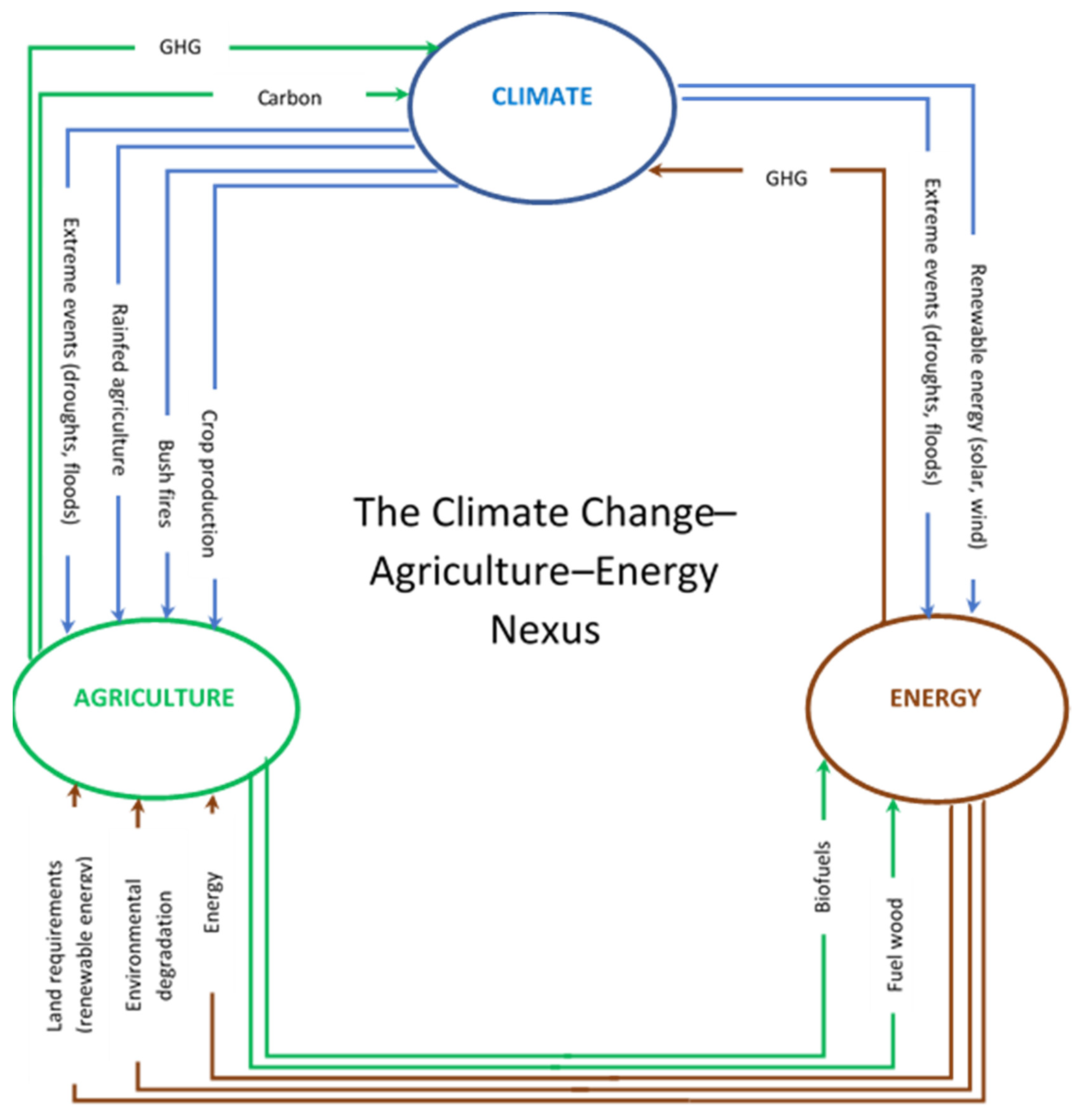
1.1. Energy, Emissions and the Agricultural Sector

Globally, energy in the agricultural sector is mainly from fossil fuels [3,21]. Primary agricultural production tends to use between 17% and 20% of total energy globally. Between one-fifth and one-quarter of this is for primary farm production, whilst the rest is for post-harvest food operations. Total global agricultural energy consumption is around 6 EJ/year (expected to increase to 9 EJ/year by 2035), with only 1 EJ/year coming from renewable energy sources [3]. This energy is mainly used for irrigation, harvesting, livestock housing, heating and cultivation. Tractors, harvesters and machinery have utilised fossil fuels at a rate of between 11.1 GJ/ha and 20.4 GJ/ha [3]. Around 0.225 EJ/year is required globally to cover 324 million hectares of irrigated land, whilst 0.05 EJ/year is required for manufacturing and delivering irrigation equipment.
Despite the declining agricultural contribution to GDP, energy use in the South African agricultural sector has been consistent, as shown in Figure 2. Electricity and coal energy use in the sector peaked at 35,052, 8 TJ and 34,020 TJ in 1998 and 2012, respectively, with lows of 15,910, 2 TJ and 16,014, 4 TJ in 1993 and 2000, respectively [22]. According to Lin and Wesseh [13], energy directly affects spending decisions of firms and households, as well as economic performance. South Africa is an energy-intensive economy, with coal alone accounting for 72% of total primary energy consumption. This, however, is not reflected in the agriculture sector, with most coal consumption being exhibited in the energy and manufacturing sectors. The country accounts for 42% of the continent’s CO2 emissions and is the world’s most carbon-intensive non-oil-producing developing country [13].
South Africa is the world’s 14th largest emitter of GHGs, mainly from coal [23]. At the 2015 Paris Agreement, nations undertook to cap emissions by 2025, at which level they will remain for a decade, and limit the increase in global temperatures to 1.5 °C by 2025. South Africa’s nationally determined contributions (NDCs), each country’s efforts at reducing national emissions and climate change adaptation, was determined at 2 °C. However, the country’s commitments are highly insufficient. In the NDCs, South Africa pledged to shift away from coal and to end the expansion of nuclear power, whilst increasing renewable energy and gas [24,25]. South Africa’s NDC is consistent with the Copenhagen Accord’s proposed reduction of emissions by 34% in 2020 and 42% in 2025 [26]. A pertinent question that arises is what effect this emission (fossil fuels) reduction will have on agricultural production? What relationship exists between CO2 emissions and agricultural production in South Africa? Not much has been documented concerning the relationship between the pledged emissions reductions and agricultural production in the country. Given that there are trade-offs between achieving the two objectives of emissions reduction and agricultural production (i.e., SDG 13 vs. SDG 1 and 2) [1], the objective of the study is to model how achieving SDGs 1 and 2 may affect the achievement of SDG 13 in South Africa. This is through predicting how poverty reduction and food security (i.e., an increase in agricultural income) might be achieved through cognizance of climate change actions.
Figure 3 shows the CO2 emissions from agriculture in South Africa from 1990 to 2012. It is shown that most of the CO2 emissions within the sector are from manure left on pastures, followed by electricity emissions and synthetic fertilisers [27]. Livestock and livestock products contribute 46–51% of agricultural income in South Africa, and have a large carbon footprint, mainly from land use and its changes (deforestation, feed production), as well as methane production [10,28,29]. The country’s main agricultural activity (livestock production) induces the most environmental degradation from the sector. Contemplating the reduction of CO2 emissions in the agricultural sector in South Africa requires climate change policy action targeting livestock production. Given that 40% of livestock farmers are smallholder farmers [30] and thus reliant on livestock production for food security and poverty reduction, the subsector exhibits trade-offs in achieving SDGs 1, 2 and 13.

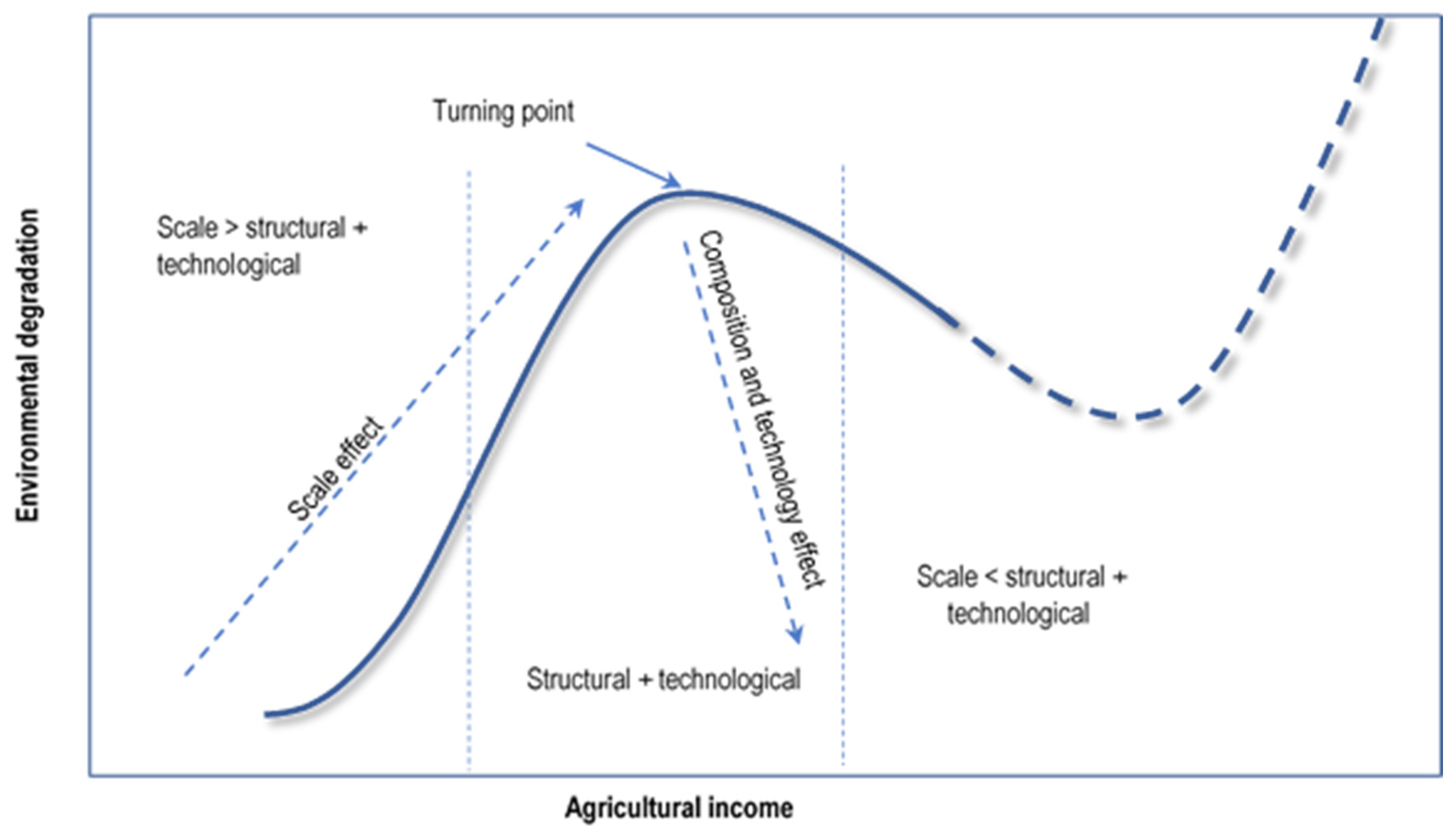
1.2. Conceptual Framework: Environmental Kuznets Curves

According to Bo [31], environmental quality indicators improve with an increase in income. However, there is a need for deeper investigation of the relationship between income and the environment. There is also a need to use data involving similar environmental involvement paths. It has also been shown that, sometimes, it is not always the case that environmental indicators improve with an increase in income, this being dependent on the indicators chosen. The objective of the study is to show the nexus between CO2 emissions and agricultural production in South Africa through environmental Kuznets curves (EKC). Environmental Kuznets curves, in the context of this study, represent a temporal relationship between agricultural GDP and climate change (emissions). This offers the advantage of tracking the likelihood of achieving SDGs 1, 2 and 13 separately, and observing how they relate to each other. This is because the EKCs depict trade-offs between environmental degradation and economic growth. Economic growth can be exhibited through food security and poverty reduction. There has been little research done in South Africa utilising EKCs, with most concentrating on developed countries. The nature of an EKC makes it a challenge to apply the test in a low- or middle-income country. Furthermore, most studies utilising the EKC focus on relationship between GDP as an economic indicator and CO2 as an environmental degradation indicator at the macrolevel [13,14,32]. Shahbaz, Kumar Tiwari, and Nasir [33], as well as Inglesi-Lotz and Bohlmann [34], utilised EKC in South Africa, concentrating on the overall economic development and growth in light of CO2 emissions, with the studies not being sectoral-based. There is a lack of studies that are sectoral-focussed, for example in agriculture as an economic indicator [35,36,37,38]. Furthermore, Kijima et al. [32] highlighted that the inverted U-shape Kuznets curve hypothesis does not always hold, depending on the country in question, the variables used and the time period considered. The study provides a way to determine the relationship between the variables used in the EKC and the agricultural sectoral level in South Africa, as intended SDG indicators. The EKC should be a precursor for developing nations to pursue economic (sectoral) growth instead of implementing pro-environment policies [39]. Economic (sectoral) growth eventually leads to attaining both environmental and economic goals, whilst pro-environment policies slow down the economic (sectoral) growth.
The conceptual framework of the study is based on environmental Kuznets curves (EKC). EKCs increase awareness of environmental changes including global warming and climate change [39]. Environmental Kuznets curves (EKC) often reflect people paying more attention to environmental issues and resolving them with the help of increasing income. Thus, while the environmental quality initially gets worse, it then improves with economic development [32]. This is based on two perspectives: (i) more attention being given to quality of life as income increases, including better environmental protection and a healthy level of consumption. The government may eventually intervene for environmental protection, improving environmental quality; and (ii) the interaction of scale, structure and technology. On the one hand, an increased scale of production induces more energy consumption and increased environmental degradation. This is also exhibited by structural changes, but to a lesser and gradually decreasing extent. On the other hand, technology and R&D then tend to improve efficiency in energy use, thereby improving environmental quality [31,32]. Thus, it follows the sequence in Figure 4. A further school of thought argues that, instead of the typical inverted U-shaped EKC, it is actually an inverted N-shape, reflecting an initial decrease in environmental degradation, followed by an increase, with an eventual decrease when the economy is developing [40].
The study will take, as its focus, the interaction of scale, structure and technology. South Africa’s agricultural sector is more developed than other SSA countries’ in terms of agricultural production and poverty reduction. This is due to the relatively large-scale and technologically advanced agricultural sector. Even though authors such as Kaika and Zervas [41] highlight that Kuznets curves have been applied in economic transformation from primary production, to secondary and tertiary, with an associated initial increase, followed by stabilisation and then a decline in degradation of the environment, the current study argues that such an approach can be taken into the agricultural sector. The focus will be on the stage of development of the agricultural sector, which in itself depicts the level of environmental degradation. If the Kuznets theory proves otherwise, it reflects that improvements within the sector have not brought (or are yet to bring) about reductions in environmental degradation. It therefore reflects that, going forward, focussing on SDGs 1 and 2 would tend to reduce the impact of SDG 13. If the Kuznets theory is exhibited, then achieving SGDs 1, 2 and 13 is possible in the inverted U-shaped model, whilst at a later stage it will be reversed in the N-shaped model.
Empirical analysis of EKCs has centred upon gas indicators harmful to people’s health like CO2, CO, NO, SO2, and the inverted U-shape was confirmed [31]. Other studies actually confirmed the inverted N-shape EKC. Some of the more recent studies on EKC are exhibited in Table 2. At the macro level, concentrating on overall GDP, EKCs have been exhibited in some studies, but not in others.

2. Materials and Methods

The study assessed the impact of agricultural production on agricultural CO2 emissions in South Africa. The study utilised time series data for the period 1990 to 2012; even though agricultural income data, as well as national CO2 emissions data, were available for South Africa up to 2018, sectoral-based CO2 emissions data were only available up to 2012, which placed a limitation on the time series dataset. The time series data were indexed to the 2004 constant figures. The data were collected from FAOSTAT and the World Bank [22,27,49]. The variables utilised included agricultural carbon dioxide emissions (CO2) as the dependent variable, with agricultural GDP, agricultural coal energy consumption and agricultural electricity energy consumption as explanatory variables. The agricultural CO2 utilised combined CO2 from fertiliser, manure applied in soil, manure left on pastures, coal and electricity.
The study utilised the method as utilised by Baek [40] as well as He and Richard [50] in estimating three models: log linear, log quadratic and log cubic:
E = F ( Y ,   Z )
E = F ( Y ,   Y 2 ,   Z )
E = F ( Y ,   Y 2 , Y 3 ,   Z ) ,
where E is the CO2 emissions from agricultural activities, Y is the agricultural GDP and Z is another explanatory variable that influences environmental degradation in agricultural production. The main objective of the study was establishing a relationship between agricultural income and agricultural CO2 emissions. The estimated models in logarithmic form are as follows:
ln ( E ) t = β 0 + β 1 ln Y t + β 4 ln A C C t + β 5 ln A E C t + ε t
ln ( E ) t = β 0 + β 1 ln Y t + β 2 ( ln Y t ) 2 + β 4 ln A C C t + β 5 ln A E C t + ε t
ln ( E ) t = β 0 + β 1 ln Y t + β 2 ( ln Y t ) 2 + β 3 ( ln Y t ) 3 + β 4 ln A C C t + β 5 ln A E C t + ε t
where t is the time period, E is the CO2 emissions from agricultural activities, Y is the real agricultural income, ACC is the agricultural coal energy consumption, AEC is the agricultural electricity consumption and ε t is the standard error term. The elasticity of CO2 with respect to agricultural income in the typical inverse U-shaped EKC form should be positive ( β 1 > 0 ), whilst the agricultural income elasticity of its square would be negative ( β 2 < 0 ). The agricultural income elasticity of its cubic would be positive ( β 3 > 0 ) for the N-shape EKC hypothesis to be true. Agricultural coal and electricity energy consumption elasticities would be expected to be positive ( β 4 β 5 ), meaning that higher coal and electricity consumption will result in higher CO2 emissions in the agricultural sector.
The study utilised the autoregressive distributive lag (ARDL) bounds test as well as the error correction model (ECM) for estimating the long-run adjustment process toward equilibrium [51,52]. This method is advantageous in that regressions can be carried out regardless of integration of I (1) or I (0), with most macroeconomic variables being either of these two orders. Another advantage is that serial correlation and endogeneity problems are removed when simultaneously taking appropriate long-run and short-run lags.
The relationships among agricultural CO2, agricultural income, agricultural coal consumption and agricultural electricity consumption in Equations (4)–(6) follow a time path before long-run nexus is achieved. Thus, Equations (4)–(6) would be written as an unrestricted error correction specification:
ln C O 2 t = α 0 + i = 1 p α i ln C O 2 t i + i = 1 p φ i ln y t i + i = 1 p δ i ln A C C t i + i = 1 p ω i ln A E C t i + λ 1 ln C O 2 t 1 + λ 2 ln y t 1 + λ 4 ln A C C t 1 + λ 5 ln A E C t 1 + ε t
ln C O 2 t = α 0 + i = 1 p α i ln C O 2 t i + i = 1 p φ i ln y t i + i = 1 p γ i ( ln y t i ) 2 + i = 1 p δ i ln A C C t i + i = 1 p ω i ln A E C t i + λ 1 ln C O 2 t 1 + λ 2 ln y t 1 + λ 3 ( ln y t 1 ) 2 + λ 4 ln A C C t 1 + λ 5 ln A E C t 1 + ε t
ln C O 2 t = α 0 + i = 1 p α i ln C O 2 t i + i = 1 p φ i ln y t i + i = 1 p γ i ( ln y t i ) 2 + i = 1 p δ i ln A C C t i + i = 1 p ω i ln A E C t i + i = 1 p i ( ln y t i ) 3 + λ 1 ln C O 2 t 1 + λ 2 ln y t 1 + λ 3 ( ln y t 1 ) 2 + λ 4 ln A C C t 1 + λ 5 ln A E C t 1 + λ 6 ( ln y t 1 ) 3 + ε t
where ε t are the new serially independent errors. The estimation procedure initially tests whether there is evidence of a cointegration relationship through the ARDL bounds test. The null hypothesis of no cointegration ( H 0 : λ 1 = λ 2 = λ 3 = λ 4 = λ 5 = λ 6 = 0 ) is tested against the alternative hypothesis ( H 1 :   λ 1 λ 2 λ 3 λ 4 λ 5 λ 6 0 ). If the F-statistics from the ordinary least squares go beyond the upper bound of the critical values provided in Pesaran et al. [51] and Pesaran and Shin [53], then the null hypothesis is rejected, exhibiting a cointegrating relationship among the variables. If the F-statistics are below the lower bound, we fail to reject the null hypothesis. When the F-statistics lie between the upper and lower critical values, the test results will be inconclusive. The next stage will be to estimate long-run coefficients of the cointegrating relation and make inferences.
The final stage will involve estimating an error correction model, taking the form of Equations (10)–(12) but including the long-run terms in the error correction variable lagged one period:
ln C O 2 t = α 0 + i = 1 p α i ln C O 2 t i + i = 1 p φ i ln y t i + i = 1 p δ i ln A C C t i + i = 1 p ω i ln A E C t i + λ e c t t 1 + ε t
ln C O 2 t = α 0 + i = 1 p α i ln C O 2 t i + i = 1 p φ i ln y t i + i = 1 p γ i ( ln y t i ) 2 + i = 1 p δ i ln A C C t i + i = 1 p ω i ln A E C t i + λ e c t t 1 + ε t
ln C O 2 t = α 0 + i = 1 p α i ln C O 2 t i + i = 1 p φ i ln y t i + i = 1 p γ i ( ln y t i ) 2 + i = 1 p δ i ln A C C t i + i = 1 p ω i ln A E C t i + i = 1 p i ( ln y t i ) 3 + λ e c t t 1 + ε t
where e c t t 1 is the error correction term represented by the OLS residual series from the long-run cointegration relationship, and the λ coefficient indicates the speed of adjustments towards this long-run equilibrium. Diagnostic tests such as the Breusch‒Godfrey serial correlation LM test, the Jarque‒Bera Test and the Breusch‒Pagan‒Godfrey Test were used to test for collinearity, normality and heteroscedasticity, respectively. Cumulative sum (CUSUM) and cumulative sum of squares (CUSUMSQ) were used to test the long- and short-run stability of the model.

3. Results and Discussion

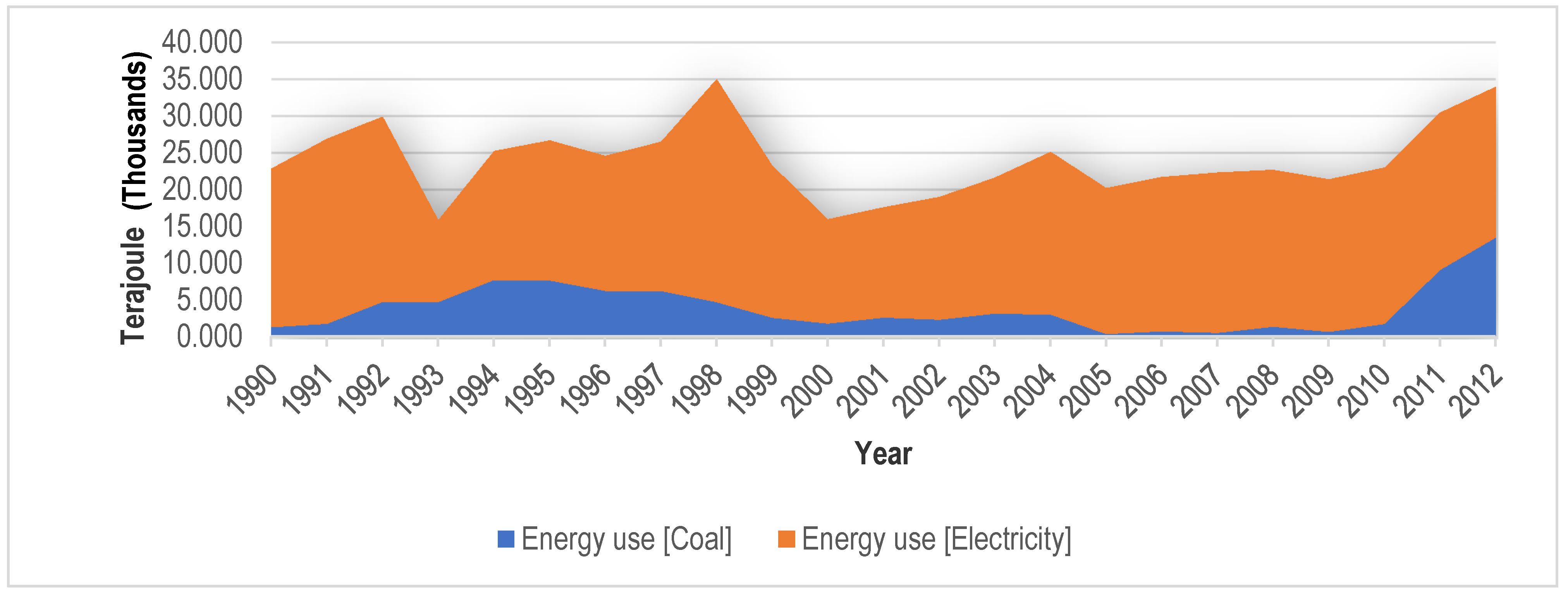
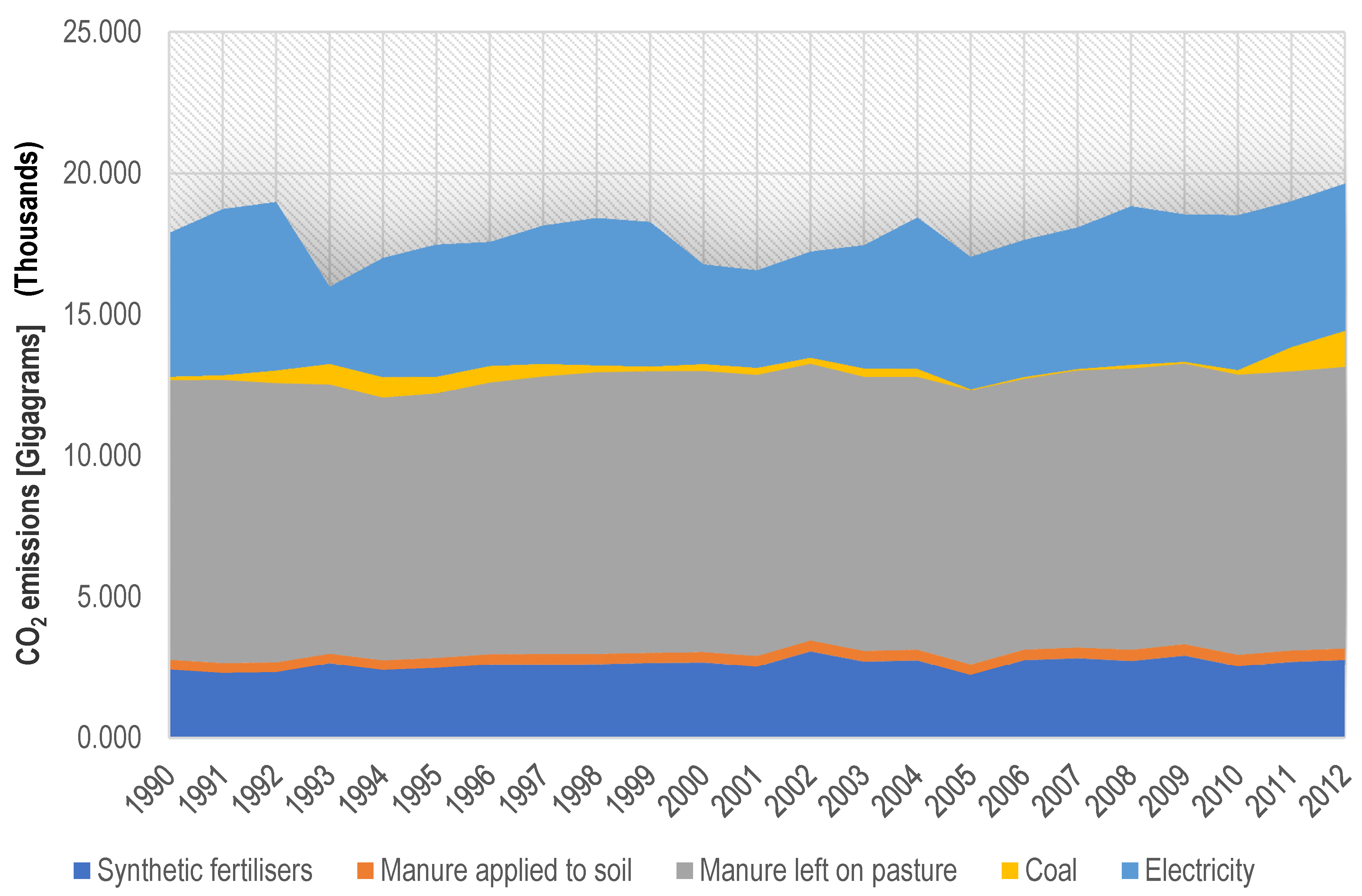
3.1. Descriptive Results

Table 3 shows that the average agricultural CO2 emissions for the 22-year period was 17,935.49 gigagrams, with a maximum of 19,093.30 gigagrams and a minimum of 15,993.25 gigagrams. The value of agricultural production has averaged R 69.17 billion, whilst coal and electricity consumption within the sector had means of 3480.81 kilojoules and 20,190.75 kilojoules, respectively. The results indicate a strong positive correlation between agricultural CO2 emissions and the value of agriculture, as well as electric energy use.

3.2. Empirical Results

Testing unit roots’ properties is necessary when applying any standard cointegration in examining the long-run relationship between variables. The augmented Dickey‒Fuller (ADF) test created by Said and Dickey [54] was used to test for unit roots. The series used in the analysis had a unit root problem. Table 4 shows that the series are integrated at different orders because AEC is of I (0), whilst the rest are I (1). The ARDL bounds test was therefore necessary for establishing the long-run relationship.
Selecting an appropriate lag length is necessary for applying the ARDL bounds testing approach to cointegration. Table 5 shows the lag selection criteria used in the study. The selection criteria was based on the Akaike information criterion (AIC) and Schwarz information criterion (SIC) statistics. The AIC is superior for small sample datasets [33]. An appropriate lag length can be used to capture dynamic linkages between series [55]. The maximum lag selections for the dependent and regressor values was 1.
Table 6 shows the results of the ARDL bounds test approach and short-run results. The results show that, for the linear, squared and cubic models, the F-statistic was greater than the critical value of the upper bound I (1), and thus there is cointegration and a long-run relationship in each of the models. In the linear model, the previous period’s CO2 emissions levels, agricultural income, agricultural coal consumption and agricultural electricity consumption contribute to the CO2 emissions levels in the next period. The table shows that a 1% increase in the previous period’s CO2 emissions causes a 0.28% increase in the next period’s CO2 emissions. A 1% increase in the agricultural income, coal consumption and electricity consumption within the sector induces a 0.023%, 0.022% and 0.18% increase in CO2 emissions, respectively.
For the squared agricultural income model, however, the linear agricultural income had a negative coefficient, whilst the squared agricultural income had a positive coefficient. In the squared agricultural income model, a 1% increase in agricultural income and the square of agricultural income induced a 0.35% reduction and 0.044% increase in CO2, respectively. This is mainly based on the characteristics within the sector, which is livestock-based, accounting for 46–51% of agricultural GDP [28]. Livestock has a large carbon footprint. Increasing income within the agricultural sector means increasing livestock production and productivity. This therefore results in increases of CO2 from manure on pastures, for instance, which is the largest CO2 emitter within the sector.
After examining the cointegration of the variables, the next stage was disclosing the impact of agricultural income, agricultural coal energy consumption and agricultural electricity energy consumption on agricultural CO2 emissions in the long run. The EKC hypothesis was not validated in the long run. The squared model showed that the linear agricultural income was negative, whilst the quadratic coefficients was positive, which is contrary to the inverted U-shaped EKC hypothesis. The cubic model also shows the linear agricultural income coefficient being negative, whilst both the quadratic and cubic coefficients were positive, which is also contrary to the inverted N-shaped EKC postulations. It is therefore deduced that the EKC hypothesis is not exhibited within the South African agricultural sector based on agricultural CO2 emissions. The results fall short of Shahbaz, Aviral, and Nasir [56] and Shahbaz et al. [33], who reported a validation of the EKC in South Africa. The differences can be explained by the scale of their studies, which were focussing on the overall economy and not sector-based. Furthermore, their studies utilised a longer time series (1965–2008), which was able to capture economic transformations over a period of time. However, Inglesi-Lotz and Bohlmann [34] also utilised a long time series (1960–2010), the same as Nasr, Gupta, and Sato [57] (1911–2010), and could not validate the EKC in South Africa. It was highlighted that the economy was still transforming through the early stages of the inverted U-shape EKC. Table 7 shows that in the linear model, agricultural income, coal energy consumption and electricity energy consumption had a significant, positive impact on agricultural CO2 emissions. In the squared model, agricultural income had a significant, negative impact on agricultural CO2 emissions, whilst the squared agricultural income, agricultural coal energy consumption and agricultural electricity energy consumption had a significant, positive influence on the agricultural CO2 emissions. For the cubic model, agricultural income had no influence on the agricultural CO2 emissions (whether linear, squared or cubic), whilst agricultural coal energy consumption and agricultural electricity energy consumption had a significant, positive influence on the agricultural CO2 emissions.
Table 7 shows that a 1% increase in the agricultural income induces a 0.03% increase and 0.28% decrease in the agricultural CO2 emissions in the linear and quadratic models, respectively. Increasing the squared agricultural income will induce a 0.035% increase in the CO2 emissions. This shows that expanding the sector is not having a significant effect in terms of CO2 emissions reduction. Thus, food security and poverty reduction (by way of agricultural income growth) are increasing CO2 emissions. There is thus a trade-off between achieving agricultural income growth (SDG 1 and 2) and reducing CO2 emissions (SDG 13). In all three models it was shown that a 1% increase in the coal energy consumption in agriculture will induce a 0.011‒0.015% increase in agricultural CO2 emissions, whilst a 1% increase in agricultural electricity consumption will result in a 0.20‒0.25% increase in agricultural CO2 emissions. This shows that, going into the future, electricity consumption will account for a large portion of the emissions from the agricultural sector. The findings were, however, different in Shahbaz et al. [33], who found that coal consumption was the major source of CO2 emissions within the South African economy. This was mainly based on the scale of the study: they concentrated on the whole economy and not a specific sector. Even though South Africa is the sixth-largest consumer of coal, its use appears to be primarily in the energy and manufacturing sectors, and not necessarily in the agricultural sector [9]. The Error Correction Term (ECT) has a negative and significant sign at the 1% level, indicating a long-run association between the variables. The ECT from the linear model shows that the change in CO2 emissions from the short run towards the long run is estimated at 71.9% every year in the linear model, whilst it is 124.7% and 125.3% for the squared and cubic models.
A pairwise Granger causality test was also performed to analyse the direction of causal relationship with regards to CO2 emissions. The causality test was necessary for establishing whether agricultural growth causes environmental degradation, or whether the emissions from agricultural activities were responsible for the sector’s growth. The pairwise Granger causality test in Table 8 shows that agricultural income, as well as its squared and cubic terms, tend to Granger cause CO2 emissions within the sector in the long run at the 1% level. Even though this was at the overall GDP level, this finding is consistent with Shahbaz et al. [33] in South Africa. However, coal and electric energy do not Granger cause CO2 emissions.

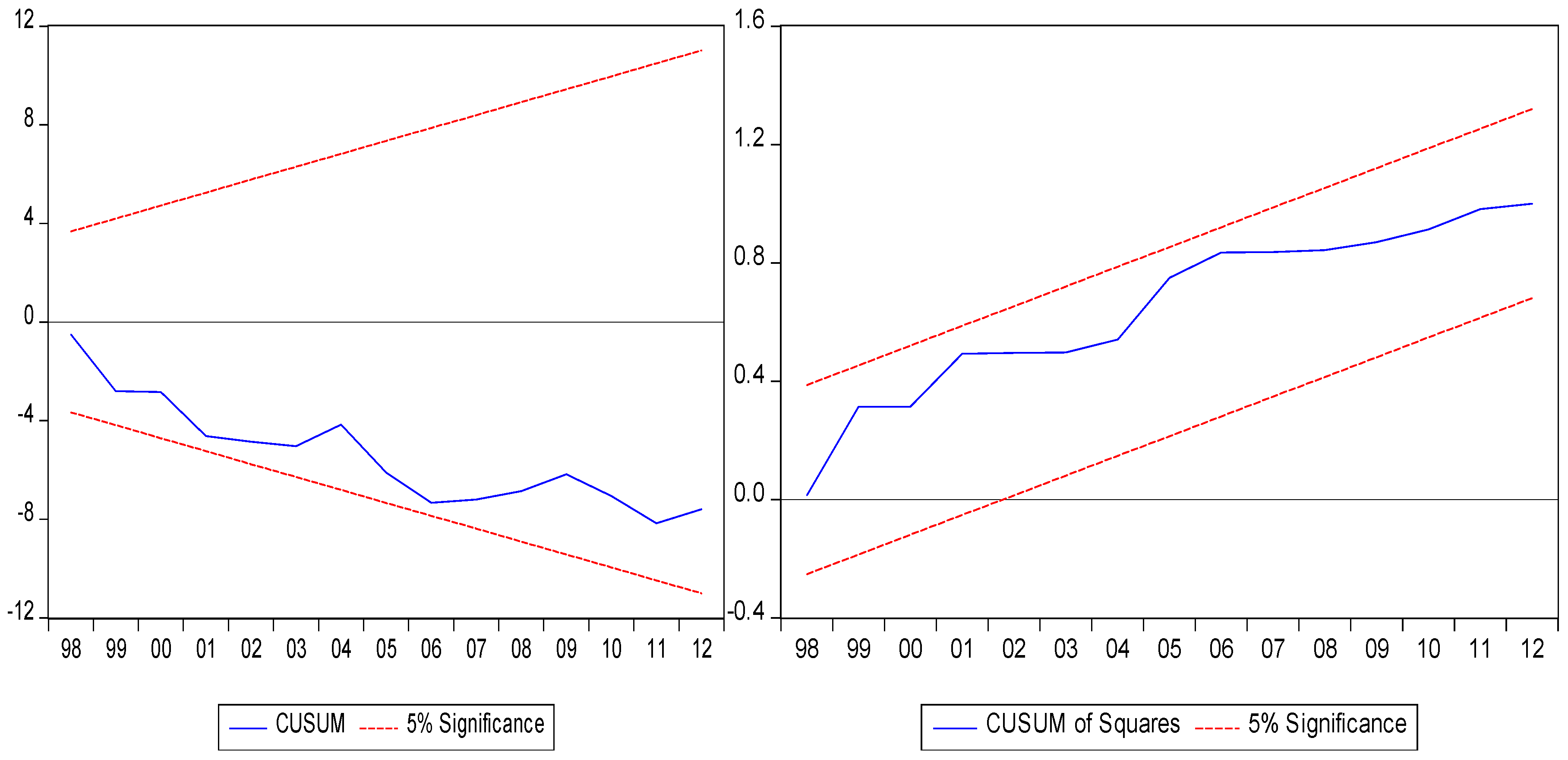
3.3. Diagnostic Tests

A sensitivity analysis indicates that the models pass all diagnostic tests. Table 9 shows the collinearity, heteroskedasticity and normality diagnostic tests. The collinearity test in all three instances shows an insignificant value, indicating no collinearity. There was also no heteroskedasticity, and normal distribution for the residual within the models. The models were thus robust.
The long-run parameter stability was tested by applying the CUSUM and CUSUM of square test. Figure 5, Figure 6 and Figure 7 show the CUSUM and CUSUM of square stability tests for the models. All the models lie within the critical bounds, and therefore confirm the stability of long-run estimates.

4. Conclusions and Recommendations

The study sought to investigate the trade-offs between SDGs 1 (poverty reduction), 2 (food security) and 13 (climate change action) through analysing the validation of environmental Kuznets curves (EKC), which examine the nexus between income and environmental degradation. The study focused on the agricultural sector in South Africa for the period 1990 to 2012, and the income that was utilised in the study was real agricultural income (2004 constant levels), whilst the indicator used for environmental degradation was agricultural CO2 emissions. The agricultural CO2 variables used in the study include agricultural income, agricultural income squared, agricultural income cubic, agricultural coal consumption and agricultural electricity consumption. The bounds testing approach was used for examining the long-run relationship between the variables. The study finds cointegration between the series in the three models (linear, squared and cubic). Furthermore, agricultural coal energy and electricity energy consumption tend to increase agricultural CO2 emissions in South Africa. The EKC hypothesis is not validated in the South African agricultural sector as there is a U-shaped EKC in the squared model, whilst no relationship was exhibited in the cubic model. Thus, as agricultural income increases, so do CO2 emissions in the South African agricultural sector. This implies that for South Africa to reduce its CO2 emissions and achieve SDG 13, the country has to sacrifice agricultural growth. This is not feasible as agriculture is required for food security and hunger reduction (SDG 2), as well as poverty reduction (SDG1). This further shows that the sector is less likely to be used to overcome environmental degradation, especially given the country’s 2 °C nationally determined contributions (NDCs). This is also exacerbated by the focus of EKC, which disregards consumption evolution and focusses on production activity [35]. Thus, promoting sectoral growth, as implied by the EKC hypothesis, will not result in simultaneous attainment of both sectoral and environmental goals. In this instance, a pro-environmental policy would be ideal for reducing the emissions from the country’s agricultural sector, as opposed to a pro-sector-growth one.
The study recommends that policies aimed at improving energy efficiency be promoted in order to decrease agricultural CO2 emissions without adversely affecting the agricultural sector’s productive capacity. To ensure the positive impact of agricultural coal energy and electricity energy on agricultural CO2 emissions, there needs to be a policy of searching for and using renewable energy (wind, solar, biodiesel fuel) within the South African agricultural sector. There is large potential for bioenergy and hydroelectricity use in the South African agricultural sector, but it will require buy-in and investment [58]. Policy makers could also increase taxes on fossil fuel use within the agricultural sector, whilst subsidising renewable energies. Furthermore, instead of focusing entirely on policy intervention, the country could also invest more in R&D for more efficient technology to be used in the sector. This could aid in reducing CO2 emissions. Ultimately, the study recommends that policy within the sector should not be linear, focussing on cause‒effect, as suggested by the EKC hypothesis. There is a need for simultaneous growth and protection of the environment [39].

Author Contributions

Conceptualization, S.N.; methodology, J.A.; validation, J.A., L.Z. and S.T.; formal analysis, S.T.; investigation, S.N.; writing—original draft preparation, S.N.; writing—review and editing, J.A.; supervision, L.Z.; project administration, S.N.

Funding

This research received no external funding.

Acknowledgments

The authors acknowledge the valuable comments from the anonymous reviewers.

Conflicts of Interest

The authors declare no conflict of interest.

References

  1. Campbell, B.M.; Hansen, J.; Rioux, J.; Stirling, C.M.; Twomlow, S.; Wollenberg, E.L. Urgent action to combat climate change and its impacts (SDG 13): Transforming agriculture and food systems. Curr. Opin. Environ. Sustain. 2018, 34, 13–20. [Google Scholar] [CrossRef]
  2. United Nations. Transforming Our World: The 2030 Agenda for Sustainable Development; United Nations: Geneva, Switzerland, 2015; Volume 16301. [Google Scholar]
  3. Sridharan, V.; Howells, M.; Ramos, E.P.; Fuso-Nerini, F.; Sundin, C.; Almulla, Y. The Climate-Land-Energy and Water Nexus: Implications for agricultural research. In Proceedings of the Science Forum 2018, Stellenbosch, South Africa, 10–12 October 2018; pp. 1–57. [Google Scholar]
  4. UNFCCC. United Nations Framework Convention on Climate Change (UNFCCC); Paris Agreement; UNFCCC: Paris, France, 2015; Report No.: Annex to decision 1/CP.21 document FCCC/CP/2015/10/Add.1; Available online: http://unfccc.int/resource/docs/2015/cop21/eng/10a01.pdf#page=24 (accessed on 23 June 2019).
  5. IPCC. Climate Change 2014: Synthesis Report: Fifth Assessment Report of the Intergovernmental Panel on Climate Change; IPCC: Geneva, Switzerland, 2014; Available online: http://www.ipcc.ch/pdf/assessment-report/ar5/syr/SYR_AR5_SPM.pdf%0A6 (accessed on 19 June 2019).
  6. Canavan, C.R.; Graybill, L.; Fawzi, W.; Kinabo, J. The SDGs will require integrated agriculture, nutrition, and health at the community level. Food Nutr. Bull. 2016, 37, 112–115. [Google Scholar] [CrossRef] [PubMed]
  7. van Noordwijk, M.; Duguma, L.A.; Dewi, S.; Leimona, B.; Catacutan, D.C.; Lusiana, B.; Öborn, I.; Hairiah, K.; Minang, P.A. SDG synergy between agriculture and forestry in the food, energy, water and income nexus: Reinventing agroforestry? Curr. Opin. Environ. Sustain. 2018, 34, 33–42. [Google Scholar] [CrossRef]
  8. Meyer, N.G.; Breitenbach, M.C.; Fenyes, T.I.; Jooste, A. The economic rationale for agricultural regeneration and rural infrastructure investment in South Africa. J. Dev. Perspect. 2007, 3, 73–83. [Google Scholar]
  9. DEA. South Africa’s Greenhouse Gas Inventory Report 2000–2010; DEA: Pretoria, South Africa, 2014. Available online: https://www.environment.gov.za/sites/default/files/docs/greenhousegas_invetorysouthafrica.pdf (accessed on 6 July 2019).
  10. USAID. Greenhouse Gas Emissions in South Africa; USAID: Washington, DC, USA, 2014. Available online: https://www.environment.gov.za/sites/default/files/docs/greenhousegas_invetorysouthafrica.pdf%0A%0A (accessed on 12 December 2017).
  11. CSIR. Final Technical Report: Intended Nationally Determined Contributions; CSIR: Pretoria, South Africa, 2015. [Google Scholar]
  12. Pegels, A. Renewable energy in South Africa: Potentials, barriers and options for support. Energy Policy 2010, 38, 4945–4954. [Google Scholar] [CrossRef]
  13. Lin, B.; Wesseh, P.K. Energy consumption and economic growth in South Africa reexamined: A nonparametric testing apporach. Renew. Sustain. Energy. Rev. 2014, 40, 840–850. [Google Scholar] [CrossRef]
  14. Menyah, K.; Wolde-Rufael, Y. Energy consumption, pollutant emissions and economic growth in South Africa. Energy Econ. 2010, 32, 1374–1382. [Google Scholar] [CrossRef]
  15. Koen, R.; Holloway, J.; Mokilane, P.; Makhanya, S.; Magadla, T. Forecasts for Electricity Demand in South Africa (2017–2050) Using the CSIR Sectoral Regression Model for the Integrated Resource Plan of South Africa (as inputs into the Integrated Resource Plan); Department of Energy: Pretoria, South Africa, 2017. Available online: http://www.energy.gov.za/IRP/irp-update-draft-report2018/CSIR-annual-elec-demand-forecasts-IRP-2015.pdf (accessed on 30 July 2019).
  16. Inglesi-Lotz, R.; Pouris, A. Energy efficiency in South Africa: A decomposition exercise. Energy 2012, 42, 113–120. [Google Scholar] [CrossRef] [Green Version]
  17. Ratshomo, K.; Nembahe, R. South African Energy Sector Report; Department of Energy: Pretoria, South Africa, 2018; pp. 2–49. Available online: http://www.energy.gov.za (accessed on 5 July 2019).
  18. Jain, S.; Jain, P.K. The rise of Renewable Energy implementation in South Africa. Energy Procedia 2017, 143, 721–726. [Google Scholar] [CrossRef]
  19. Rafey, W.; Sovacool, B.K. Competing discourses of energy development: The implications of the Medupi coal-fired power plant in South Africa. Glob. Environ. Chang. 2011, 21, 1141–1151. [Google Scholar] [CrossRef]
  20. Walwyn, D.R.; Brent, A.C. Renewable energy gathers steam in South Africa. Renew. Sustain. Energy Rev. 2015, 41, 390–401. [Google Scholar] [CrossRef] [Green Version]
  21. Bundschuh, J.; Chen, G. Sustainable Energy Solutions in Agriculture; CRC Press: Boca Raton, FL, USA, 2014. [Google Scholar]
  22. FAOSTAT. Agriculture Energy Consumption—South Africa. 2019. Available online: http://www.fao.org/faostat/en/#data/GT (accessed on 1 July 2019).
  23. McSweeney, R.; Timperely, J. The Carbon Brief Profile—South Africa. 2019. Available online: https://www.carbonbrief.org/the-carbon-brief-profile-south-africa (accessed on 28 June 2019).
  24. DEA. South Africa’s Intended Nationally Developed Contribution; DEA: Pretoria, South Africa, 2015. Available online: https://www.environment.gov.za/sites/default/files/docs/sanational_determinedcontribution.pdf (accessed on 16 June 2019).
  25. Climate Smart Tracker. South Africa—Country Summary. 2019. Available online: https://climateactiontracker.org/countries/south-africa/ (accessed on 27 June 2019).
  26. StatsSA. Sustainable Development Goals: Indicator Baseline Report 2017—South Africa; Statistics South Africa: Pretoria, South Africa, 2017.
  27. FAOSTAT. Agricultural Total Emission—South Africa 2019. Available online: http://www.fao.org/faostat/en/#data/GT (accessed on 1 July 2019).
  28. DAFF. Trends in the Agricultural Sector; DAFF: Pretoria, South Africa, 2018. Available online: https://www.daff.gov.za/Daffweb3/Portals/0/Statistics and Economic Analysis/Statistical Information/Trends in the Agricultural Sector 2017.pdf (accessed on 28 June 2019).
  29. Meissner, H.H.; Scholtz, M.M.; Engelbrecht, F.A. Sustainability of the South African livestock sector towards 2050 part 2: Challenges, changes and required implementations. S. Afr. J. Anim. Sci. 2013, 43, 298–319. [Google Scholar] [CrossRef]
  30. StatsSA. Community Survey 2016 Agricultural Households; StatsSA: Pretoria, South Africa, 2016. Available online: http://www.statssa.gov.za/?page_id=964 (accessed on 28 June 2019).
  31. Bo, S. A literature survey on environmental Kuznets curve. Energy Procedia 2011, 5, 1322–1325. [Google Scholar] [CrossRef]
  32. Kijima, M.; Nishide, K.; Ohyama, A. Economic models for the environmental Kuznets curve: A survey. J. Econ. Dyn. Control 2010, 34, 1187–1201. [Google Scholar] [CrossRef]
  33. Shahbaz, M.; Kumar Tiwari, A.; Nasir, M. The effects of financial development, economic growth, coal consumption and trade openness on CO2 emissions in South Africa. Energy Policy 2013, 61, 1452–1459. [Google Scholar] [CrossRef]
  34. Inglesi-Lotz, R.; Bohlmann, J. Environmental Kuznets curve in South Africa: To confirm or not to confirm? In Proceedings of the Ecomod Conference, Bali, Indonesia, Bali, Indonesia, 6–18 July 2014; pp. 1–17. [Google Scholar]
  35. Kaika, D.; Zervas, E. The Environmental Kuznets Curve (EKC) theory. Part B: Critical issues. Energy Policy 2013, 62, 1403–1411. [Google Scholar] [CrossRef]
  36. Lin, B.; Omoju, O.E.; Nwakeze, N.M.; Okonkwo, J.U.; Megbowon, E.T. Is the environmental Kuznets curve hypothesis a sound basis for environmental policy in Africa ? J. Clean. Prod. 2016, 133, 712–724. [Google Scholar] [CrossRef]
  37. Parker, H. Understanding Patterns of Climate Resilient Economic Development in Rwanda; ODI Annual Report: London, UK, 2015. [Google Scholar]
  38. Bouvier, R.A. Air Pollution and Per Capita Income: A Disaggregation of the Effects of Scale, Sectoral Composition, and Technological Change; Report No.: Working Paper, Series; Brock, W.A., Ed.; University of Massachusetts at Amherst: Boston, MA, USA, 2004; p. 84. [Google Scholar]
  39. Gill, A.R.; Viswanathan, K.K.; Hassan, S. The Environmental Kuznets Curve (EKC) and the environmental problem of the day. Renew. Sustain. Energy Rev. 2018, 81, 1636–1642. [Google Scholar] [CrossRef]
  40. Baek, J. Environmental Kuznets curve for CO2 emissions: The case of Arctic countries. Energy Econ. 2015, 50, 13–17. [Google Scholar] [CrossRef]
  41. Kaika, D.; Zervas, E. The Environmental Kuznets Curve (EKC) theory-Part A: Concept, causes and the CO2 emissions case. Energy Policy 2013, 62, 1392–1402. [Google Scholar] [CrossRef]
  42. Balaguer, J.; Cantavella, M. Estimating the environmental Kuznets curve for Spain by considering fuel oil prices (1874–2011). Ecol. Indic. 2016, 60, 853–859. [Google Scholar] [CrossRef]
  43. Alam, M.M.; Murad, M.W.; Noman, A.H.; Ozturk, I. Relationships among carbon emissions, economic growth, energy consumption and population growth: Testing Environmental Kuznets Curve hypothesis for Brazil, China, India and Indonesia. Ecol. Indic. 2016, 70, 466–479. [Google Scholar] [CrossRef]
  44. Apergis, N. Environmental Kuznets curves: New evidence on both panel and country-level CO2 emissions. Energy Econ. 2016, 54, 263–271. [Google Scholar] [CrossRef]
  45. Al-Mulali, U.; Ozturk, I. The investigation of environmental Kuznets curve hypothesis in the advanced economies: The role of energy prices. Renew. Sustain. Energy Rev. 2016, 54, 1622–1631. [Google Scholar] [CrossRef]
  46. Ahmad, N.; Du, L.; Lu, J.; Wang, J.; Li, H.Z.; Hashmi, M.Z. Modelling the CO2 emissions and economic growth in Croatia: Is there any environmental Kuznets curve? Energy 2017, 123, 164–172. [Google Scholar] [CrossRef]
  47. Özokcu, S.; Özdemir, Ö. Economic growth, energy, and environmental Kuznets curve. Renew. Sustain. Energy Rev. 2017, 72, 639–647. [Google Scholar] [CrossRef]
  48. Churchill, S.A.; Inekwe, J.; Ivanovski, K.; Smyth, R. The Environmental Kuznets Curve in the OECD: 1870–2014. Energy Econ. 2018, 75, 389–399. [Google Scholar] [CrossRef]
  49. World Bank. World Development Indicators: Agriculture, Forstery and Fishing (% added of GDP)—South Africa. 2019. Available online: https://data.worldbank.org/indicator/NV.AGR.TOTL.ZS?locations=ZA&view=chart (accessed on 3 July 2019).
  50. He, J.; Richard, P. Environmental Kuznets curve for CO2 in Canada. Ecol Econ. 2010, 69, 1083–1093. [Google Scholar] [CrossRef]
  51. Pesaran, M.H.; Pesaran, B. Working with Microfit 4.0: Interactive Econometric Analysis; Oxford University Press: Oxford, UK, 1997. [Google Scholar]
  52. Pesaran, M.H.; Shin, Y.; Smith, R.J. Bounds testing approaches to the analysisof level relationships. J. Appl. Econom. 2001, 16, 289–326. [Google Scholar] [CrossRef]
  53. Pesaran, M.H.; Shin, Y. An autoregressive distributed lag modelling approachto cointegration analysis. In Econometrics and Economic Theoryin 20th Century: The Ragnar Frisch Centennial Symposium; Strom, S., Ed.; Cambridge University Press: Cambridge, UK, 1997. [Google Scholar]
  54. Said, S.E.; Dickey, D.A. Testing for unit roots in autoregressive-moving averagemodels of unknown order. Biometrika 1984, 71, 599–607. [Google Scholar] [CrossRef]
  55. Lütkepohl, H. Structural Vector Autoregressive Analysis for Cointegrated Vari-Ables; Springer: Heidelberg/Berlin, Germany, 2006; pp. 73–86. [Google Scholar]
  56. Shahbaz, M.; Aviral, T.; Nasir, M. The Effects of Financial Development, Economic Growth, Coal Consumption and Trade Openness on Environment Performance in South Africa; Federal Bureau of Statistics, Government of Pakistan: Islamabad, Pakistan, 2011.
  57. Nasr, B.A.; Gupta, R.; Sato, R.J. Is there an Environmental Kuznets Curve for South Africa? A co-summability approach using a century of data. Energy Econ. 2015, 52, 136–141. [Google Scholar] [CrossRef] [Green Version]
  58. Shahbaz, M.; Adebola, S.; Ozturk, I. Environmental Kuznets Curve hypothesis and the role of globalization in selected African countries. Ecol. Indic. 2016, 67, 623–636. [Google Scholar] [CrossRef] [Green Version]
Figure 1. The climate change‒agriculture‒energy nexus. Adapted from Sridharan et al. [3].
Climate 07 00108 g001
Figure 2. Energy use in South Africa’s agriculture sector (the energy use does not take into account energy from methane and fuel oils, which contribute more than 50% of energy use in South Africa’s agricultural sector [17]). Source: FAOSTAT [22].
Climate 07 00108 g002
Figure 3. Carbon dioxide emissions from the South African agricultural sector. Source: FAOSTAT [27].
Climate 07 00108 g003
Figure 4. Kuznet curves model.
Climate 07 00108 g004
Figure 5. CUSUM and CUSUM of squares test for the linear model.
Climate 07 00108 g005
Figure 6. CUSUM and CUSUM of squares test for the squared model.
Climate 07 00108 g006
Figure 7. CUSUM and CUSUM of squares test for the cubic model.
Climate 07 00108 g007
Table 1. Drivers, trends and challenges to energy use in South Africa.
DriversKey TrendsFuture Challenges
Population increase and urbanizationIncrease in the amount of energy use and energy in food production [12]-Maintaining energy use whilst increasing food production
Growing energy demandIncreased energy use in agriculture, manufacturing, households, etc. [13,14]-Providing adequate energy to agriculture without increasing pollution
-Competing interest in terms of energy use between agriculture and other sectors of the economy
Increase in the amount of energy use in food productionIncreased energy use in agricultural and manufacturing sectors [15,16]-Ensuring sufficient, reliable and efficient energy for agriculture
Economic growth, industrialization and urbanizationIncreasing non-renewable energy importation [12,17,18,19,20]-Ensuring stable and quality energy supply for food production
-Promoting private sector involvement in renewable energy utilisation for food production
Table 2. Recent studies on environmental Kuznets curves.
AuthorPeriodCountry/Region/OrganizationMethodologyVariables Used in the StudyEKC Hypothesis
Balaguer and Cantavella [42]1874–2011SpainAutoregressive distributed lag (ARDL) bounds test approach and error correction model (ECM)Per capita CO2, GDP, crude oil pricesExhibited
Alam, Murad, Noman, and Ozturk [43]1970–2012Brazil, China, India and IndonesiaARDL and ECMPer capita CO2, GDP, energy, Trade opennessExhibited in India, but not in Brazil, China and Indonesia
Apergis [44]1960–201315 OECD countriesCommon correlated effects and panel quantile cointegration testEmissions, per capita GDPMixed results
Al-Mulali and Ozturk [45]1990–201227 CountriesKao and Fisher cointegration and VECMCO2, GDP, renewable energy consumption, non-renewable energy consumption, trade, population, energy pricesExhibited
Ahmad et al. [46]1992–2011CroatiaARDL and VECMCO2, GDPExhibited
Özokcu and Özdemir [47]1980–201026 OECD countries and 52 emerging countriesPolynomial (cubic) regression modelCO2 per capita, GDP per capita, energy use per capitaMixed results
Churchill, Inekwe, Ivanovski, and Smyth [48]1870–201420 OECD countriesPanel cointegration, mean group estimator (MGE), common corelated mean group (CCEMG), augmented mean group (AMG) and pooled MG (PMG) estimatorCO2, GDP, trade, population, financial developmentMixed results
Table 3. Descriptive statistics.
CO2 Emissions (Gigagrams)Gross Value of Agriculture (R Million)Coal Energy (Kilojoules)Electricity Energy (Kilojoules)
Mean17,935.4969,168.653840.80920,190.75
Median18,093.3052,185.602605.80020,718.00
Maximum19,646.0716,8591.113,467.6030,357.20
Minimum15,993.2520,198.00361.000011,188.80
Std Dev.899.991144,950.373294.0363915.104
Skewness−0.2463520.7906011.2601090.133680
Kurtosis2.4467912.3939594.2210924.191326
Correlation
CO2 emissions1.000
Gross value of agriculture0.5251.000
Coal energy0.2640.1421.000
Electricity energy0.7470.095−0.0301.000
Table 4. Augmented Dickey‒Fuller unit root test.
ADF Statistics
I (0)
ADF Statistics
I (1)
ln C O 2 t −2.48−5.44 ***
ln Y t −2.33−5.27 ***
( ln Y t ) 2 0.81−5.24 ***
( ln Y t ) 3 1.68−4.87 ***
ln A C C t −1.61−4.66 ***
ln A E C t −3.78 **
Critical values1%−3.809
5%−3.021
10%−2.650
Max lag = 2; Schwarz info. criterion; Sig at ** 5%, *** 1%.
Table 5. Lag selection criterion.
AICSC
Lag012012
ln C O 2 t −3.03−3.12 *−3.04−2.98−3.02 *−2.89
ln Y t 1.92−1.98 *−1.91.97−1.89 *−1.75
( ln Y t ) 2 6.292.48 *2.566.342.58 *2.70
( ln Y t ) 3 10.126.41 *6.4810.176.51 *6.63
ln A C C t 2.892.38 *2.462.942.48 *2.61
ln A E C t −0.22 *−0.22−0.22−0.22 *−0.12−0.07
Sig at * 5%.
Table 6. Bounds test and short-run relationship.
Variable Climate 07 00108 i001 Climate 07 00108 i002 Climate 07 00108 i003
ln C O 2 t (-1)0.28 (2.91) **–0.25 (–1.31)–0.26 (–1.24)
ln Y t 0.023 (2.97) ***–0.35 (–3.18) ***–0.20 (–0.12)
( ln Y t ) 2 0.044 (3.46) ***0.0079 (0.019)
( ln Y t ) 3 0.0028 (0.090)
ln A C C t 0.022 (3.72) ***0.014 (3.26) ***0.013 (2.06) *
ln A C C t (-1)–0.011 (–1.67)
ln A E C t 0.18 (8.28) ***0.16 (9.03) ***0.16 (8.61) ***
ln A E C t (-1) 0.087 (2.22) **0.088 (2.14) *
C 5.20 (5.95) ***5.01 (2.13) *1
R-squared0.8876830.9308610.930900
Adjusted R-squared0.8525840.9032050.896351
F-statistic25.29077 ***33.65891 ***26.94370 ***
Durbin‒Watson statistic2.4342742.2144192.210267
F-bounds test
F-statistic28.1111.699.09
I (0)I (1)I (0)I (1)I (0)I (1)
10%2.723.772.453.522.263.35
5%3.234.352.864.012.623.79
2.5%3.694.893.254.492.964.18
1%4.295.613.745.063.414.68
Sig. at * 10%, ** 5%, *** 1%; t-values in parentheses.
Table 7. Error correction model and long-run relationship.
Variable Climate 07 00108 i001 Climate 07 00108 i002 Climate 07 00108 i003
ln Y t 0.032 (3.06) ***–0.28 (–3.58) ***–0.12 (–0.11)
( ln Y t ) 2 0.035 (3.95) ***0.0063 (0.019)
( ln Y t ) 3 0.0022 (0.090)
ln A C C t 0.015 (2.00) *0.011 (3.12) ***0.011 (1.9) *
ln A E C t 0.25 (5.97) ***0.20 (10.06) ***0.20 (9.70) ***
CointEq (-1)–0.719 ***–1.247 ***–1.253 ***
Sig. at * 10%, ** 5%, *** 1%; t-values in parentheses.
Table 8. Pairwise Granger causality test.
F-StatisticProb.
ln Y t does not Granger cause ln C O 2 t 3.151220.0702
( ln Y t ) 2 does not Granger cause ln C O 2 t 3.076310.0741
( ln Y t ) 3 does not Granger cause ln C O 2 t 3.118330.0718
ln A C C t does not Granger cause ln C O 2 t 0.576360.5732
ln A E C t does not Granger cause ln C O 2 t 0.863140.4406
Table 9. Residual diagnostic tests.
Climate 07 00108 i001 Climate 07 00108 i002 Climate 07 00108 i003
F-StatProb.F-StatProb.F-StatProb.
Breusch‒Godfrey serial correlation LM test2.2087480.14670.7110480.50930.9480050.4147
Breusch‒Pagan‒Godfrey heteroskedasticity test2.0584140.12452.1252510.11071.7332810.1804
Jarque‒Bera normality test2.9621890.2273890.98986240.6096850.9874040.610363

