Validation and Improvement of the WRF Building Environment Parametrization (BEP) Urban Scheme

Department of Atmospheric and Oceanic Science, University of Maryland-College Park, Maryland, MD 20742, USA
*
Author to whom correspondence should be addressed.
Climate 2019, 7(9), 109; https://0-doi-org.brum.beds.ac.uk/10.3390/cli7090109
Submission received: 7 May 2019
/
Revised: 12 August 2019
/
Accepted: 28 August 2019
/
Published: 10 September 2019
Abstract
:The building environment parameterization scheme (BEP) is a built-in “urban physics” scheme in the weather research and forecasting (WRF) model. The urbanized College Park (CP) in Maryland state (MD) in the United States (US) covers an approximate land area of 14.8 km2 and has a population of 32,000 (reported by The United States Census Bureau, as of 2017). This study was an effort to validate and improve the BEP urban physics scheme for a small urban setting, College Park, MD. Comparing the WRF/BEP-simulated two-meter air temperatures with the local rooftop WeatherBug® observations and with the airport observations, systemic deficiencies in BEP for urban heat island effect simulation are evident. Specifically, WRF/BEP overestimates the two-meter air temperature by about 10 °F during clear summer nights and slightly underestimates it during noon of the same days by about 1–3 °F. Similar deficiencies in skin temperature simulations are also evident in WRF/BEP. Modification by adding an anthropogenic heat flux term resulted in better estimates for both skin and two-meter air temperatures on diurnal and seasonal scales.
1. Introduction
Urbanization effects have been widely reported across the globe. The impact of a typical urban terrain on the overlying atmosphere is not only local but also regional, depends on the city size, population density, and atmospheric general circulation conditions. The urban heat island effect (UHI), for example, has been observed and studied over different cities with apparent effects of the urban canopy on the regional energy budget [1,2,3,4]. However, challenges in urban modelling still remain, given the enormous urban heterogeneities and their impacts on thermodynamic parameters as well as the physical processes. Most of the previous studies are for large urbanization regions. How a small urban setting disturbs the surface temperature and how to simulate such disturbances in a regional model are the focuses of this study.
“Anthropogenic” heat flux is one of the important reasons for UHI and thus needs to be adequately modeled [5,6,7]. Vourlitis et al. 2008 [8] suggested empirically modeling the anthropogenic contributions to the overall heat flux to get an improved estimate of land and atmospheric properties over urban canopy. In addition, Moriwaki and Kanda (2004) [9] speculated the significant influences of the buildings, roads, and other urban canopy structures in modifying the net radiative input and developing a localized heat reservoir to hold an excess amount of heat over the urban canopy.
Jin and Shepherd (2005) and Jin and Dickinson (2010) highlighted the significance of the inclusion of satellite-based urban observations into the climate models [10,11]. They also concluded that due to the significant impact of the UHI effect on skin temperatures, the radiative transfer equation gets imbalanced and this needs to be accounted for by considering “urban heat flux” [12,13,14]. Spronken-Smith and Oke (1999) presented a detailed overview of the causes and effects of UHI [15]. They provided a well-accepted view of how the temperature contrast between a city and its surrounding rural areas affects the urban airflow, urban temperature profile, and the entire urban boundary layer structure. These findings are consistent with the studies using real data over a number of different cities [16,17,18,19].
There has been a significant amount of progress in recent urban modelling. A number of studies [10,20,21] have used the same urban scheme (the single-layer urban canopy model, SLUCM) coupled with the weather research and forecast (WRF) model [22]. Other studies use the building environment parametrization (BEP) scheme along with WRF. For example, Zhang et al. (2017) performed an analysis of the UHI effect through conducting control-runs (without implementing SLUCM) and sensitivity runs (with SLUCM) in WRF simulations and noted that the sensitivity runs were able to better simulate the UHI effect, by comparing the model results with the ground and satellite observations, than the control runs [22]. Arnfield (2003) [21] suggested differences in the roughness length over urban and rural regions. They attributed this to the prevalent UHI effect over the given urban region. Arnfield (2003) suggested that compared to the two-meter air temperature, the skin temperature plays a much more significant role in governing the urban meteorological processes, as the skin temperature over an urban canopy is directly dependent on the building coverage, density, and height, and is relatively independent of the atmosphere covering the region [21].
Several studies [22,23,24,25] have developed parametrization to make modelling and observations consistent. These works led to the development of parametrization schemes for the surface flux, a parameter for the surface boundary layer profile. Sun and Mahrt (1995) determined the differences between the air temperature (the aerodynamic temperature) and the “surface radiative temperature” or the skin temperature (estimated from the surface energy balance) [26]. The differences observed between these two temperatures were related to land cover type and surface albedo, and over an urban canopy region, the difference was larger during midday hours.
Jin et al. (2005) (JI) thoroughly inspected the influence of the urban system on climate change [27]. In other previous studies [28,29,30,31] which analyzed the UHI effect extensively, the dependence of the UHI effect on the surface temperatures, albedos, and emissivity was demonstrated. JI illustrated this dependence on different urban settings (e.g., Beijing, Phoenix, New York) using high quality satellite datasets. In particular, JI also inferred UHI from skin temperature and revealed that UHI is evident in both the daytime and nighttime. Wong et al. (2017) recently performed experiments to show that daytime urban temperatures can be more than surrounding rural temperatures by 3–5°C, and that the nighttime urban temperatures can exceed by approximately 12 °C [32]. This is essentially due to the buildings and other urban structures trapping solar energy and re-emitting in the form of longwave radiation.
Zhang et al. (2017) provide a strong background for analyzing the urban surface temperature dynamically and thermodynamically as a whole [22]. The MUC [33], which is based on one of the two urban schemes—the building environment parametrization (BEP) scheme or the building energy model (BEM) scheme, has been validated using satellite and ground observations and generally performed better in urban regions due to relatively complex treatments of urban canyons.
Previous studies, however, were mostly focused on large urban regions. Does a small city have similar UHI and how to simulate a small city’s UHI effect? This study focuses on a small urban region, urbanized College Park (CP) in Maryland state (MD) in the United States (US) which has approximate land area of 14.8 km2 with a population of 32,000 (reported by The United States Census Bureau, as of 2017). Implementation of the BEP coupled with the WRF/Noah-land surface model (Noah-LSM), this study plans to validate and improve the BEP model’s capability for determining small urban effects. Specifically, in this study, we performed controlled run (without SLUCM or BEP) and sensitivity run (with SLUCM and BEP, respectively) simulations on WRF and compared the two-meter air temperature and skin temperature results against each other. In summary, in this study, we:
- modified the ground heat fluxes in the BEP by adding a new anthropogenic heat flux term and compared the results for the two-meter air temperatures and skin temperatures
- validated the above model outputs using ground-based observations obtained from the local “WeatherBug®” observations and nearby College Park airport ground observations.
2. Model Description and Study Methods
2.1. Model Specifics—BEP Urban Physics Scheme
The BEP urban physics scheme is an urban canopy model (i.e., multilayer urban canopy model) which is coupled with the land surface model (i.e., Noah) in the WRF framework. BEP provides the set of options to be selected for the study domain to parameterize the governing physical and dynamical interactions between the urban surface and the atmosphere [34,35,36]. BEP differs from SLUCM because it carefully considers the dynamical and radiative features of the urban canopy (i.e., roads, building rooftops and walls, concrete) using empirical expressions and thus has improved interpretation of physical and dynamical interactions. By dividing the urban canopy into several vertical layers and calculating an effective horizontal surface area at each vertical level using empirical expressions, BEP estimates surface energy fluxes, components of turbulent kinetic energy, the coefficients of absorptivity and reflectivity, and emissivity at that vertical level [34]. Another feature of the BEP scheme is that it considers the impact of the shading induced by building heights within the urban canopy which leads to, in part, the UHI effect over the canopy [36]. Compared to BEP scheme, the SLUCM follows a more simplistic approach of bulk parameterization with regards to estimation of urban properties. As a result, it is expected to better estimate heat fluxes and related properties than SLUCM.
2.2. Physics and Dynamics Involved
2.2.1. Radiation Budget and Fluxes
Changnon (1978) gave a fundamental governing equation to estimate the total available radiative energy [28], which has been repeatedly used in studies since [29,37,38,39] (Rnet) in terms of the incoming and outgoing shortwave (S) and longwave radiation (L),
This total available radiative energy is kept within an urban surface determined by surface albedo and emissivity. Generally, urban surfaces have lower albedo and emissivity than rural areas [40], leading to higher absorption of solar radiation and less longwave emission [8]. The above Equation (1) is the standard expression that provides an estimate of the net radiative surplus or deficit over an urban canopy. In a normal land surface, net radiative energy is the primary driving force for all physical processes, which can be partitioned into surface energy flux components in the surface energy flux balance:
where Rneti in Equation (2) is estimated from the budget expression and may be different, in terms of value, from the net flux estimated by Equation (1). H and LE are respectively the sensible and latent heat fluxes, and G is the surface (ground) heat flux. Following Moriwaki and Kanda (2004), ∆S represents the storage term, which accounts for the heating of objects other than the ground (large urban structures i.e., buildings), which is estimated indirectly by modifying the sensible, latent, and ground heat fluxes in the flux equation [9]. More importantly, in urban systems, the heat contribution of anthropogenic sources (F) has been found to be noticeable [6,7,41], resulting in a modified urban surface energy balance:
where F, the anthropogenic flux, is fundamentally human activity-induced heat fluxes, such as those produced by friction of tires on the road, traffic emissions, and air conditioning usage. This amount of flux in an urban region must be included in energy budget needs but is ignored in the BEP model. This study suggests an empirical equation for the anthropogenic flux.
Rnet = S ↓ − S ↑ + L ↓ − L↑
Rneti= H + LE + G + ∆S
Rnet + F = H + LE + G + ∆S
2.2.2. Anthropogenic Heat Flux
In this study, the fluxes from the roads, building walls, and building roofs were re-estimated and were used to speculate the fluxes in a combined urban and rural region:
where rlup is the net upward longwave emissions from the ground, rlemit is the longwave emissions term from the ground, and rld is the net downward longwave radiations being received at the ground.
where grdflxs is the ground flux from the road, grdflxb is the ground flux from the building, ws is the width of the road, and wb is the effective width of the building in the urban regions. The sum of these two terms is the net urban ground flux,
rlup = rlemit − rld
grdflxs = gfl +ws/(ws + wb)
grdflxb = gfl+wb/(ws + wb)
gurb = grdflxs + grdflxb
The overall ground heat flux and sensible heat flux are the summation of the urban ground heat flux and rural ground heat flux terms,
where grdflx is the total ground heat flux in a given region (urban + rural), frcurb is the urban fraction (which is a prescribed variable), and sh is the total sensible heat flux. On the right-hand side of Equation (8), the first term is named “grdflxurb”. Hence, the second term can be called “grdflxrural”. As with Equation (9), the first team on the right side is “shrub” and the second term is “shrural”.
grdflx = frcurb × gurb + (1 − frcurb) × gsoil
sh = frcurb × shurb + (1 − frcurb) × shsoil
The model computes the emissivity over the urban and rural components of a given region. These can then be conveniently used to determine the net emissivity (ε) of the region as,
ε = frcurb × εurb + (1 − frcurb) × εrural
In addition to this, the transport of heat via latent heat flux term computed by the following equation,
where qfx stands for moisture flux,
where lh is the net latent heat flux and lv is the specific latent heat for vaporization of water.
qfx = frcurb × qfxurb + (1 − frcurb) × qfxrural
lh = qfx x lv
In our study, the anthropogenic heat flux F in Equation (3) was added as a new term in the original BEP model to capture the human activity-induced heat fluxes. Assessing the amount of F is ongoing research. F should be a function of city population, living style, city size, location, and season. In this work, to simplify our calculation, F is chosen proportional to the heat fluxes:
F = 0.1 × (grdflxurb +shurb)
3. Data and Field Specifics
The control runs and sensitivity runs were performed for four different days corresponding to four different seasonal configurations—05/01/2017 (during the late spring), 08/01/2017 (during mid-summer), 10/27/2017 (during mid-fall), and 01/23/2018 (during late winter). In addition, in order to demonstrate the model capabilities for cloudy days, one “cloudy” day (overcast conditions) on 09/27/2017 was also simulated. The total land coverage (urban + rural) of College Park, Maryland (MD) is approximately 14.8 km2, with the simulations performed over a set of domains via two-way nesting with 3.6 km, 1.2 km, and 0.4 km resolution for the three domains, respectively. WRF runs were performed for “No urban”, “SLUCM”, “BEP” urban physics schemes, and “modified BEP” model (WRF options 0, 1, and 2, respectively). The experiments used the NCEP global forecasting system (GFS) 0.25 degree three-hourly analysis and forecast data for boundary and initial conditions. Since the BEP model does not include anthropogenic flux induced by traffic, air conditioning, and other human activities, we modified BEP by adding this flux into the model.
The WeatherBug® site (hereafter WeatherBug) at the University of Maryland, College Park campus measures two-meter air temperature at 5 second intervals and was sampled to one hour in this study. In addition, the two-meter air temperature measured at the College Park airport via a standard weather station was also used to represent rural temperature. College Park airport is only two miles away from the university campus and has dense vegetation coverage. The campus is covered by buildings, roads, and parking lots and is thus a small urban setting.
4. Results
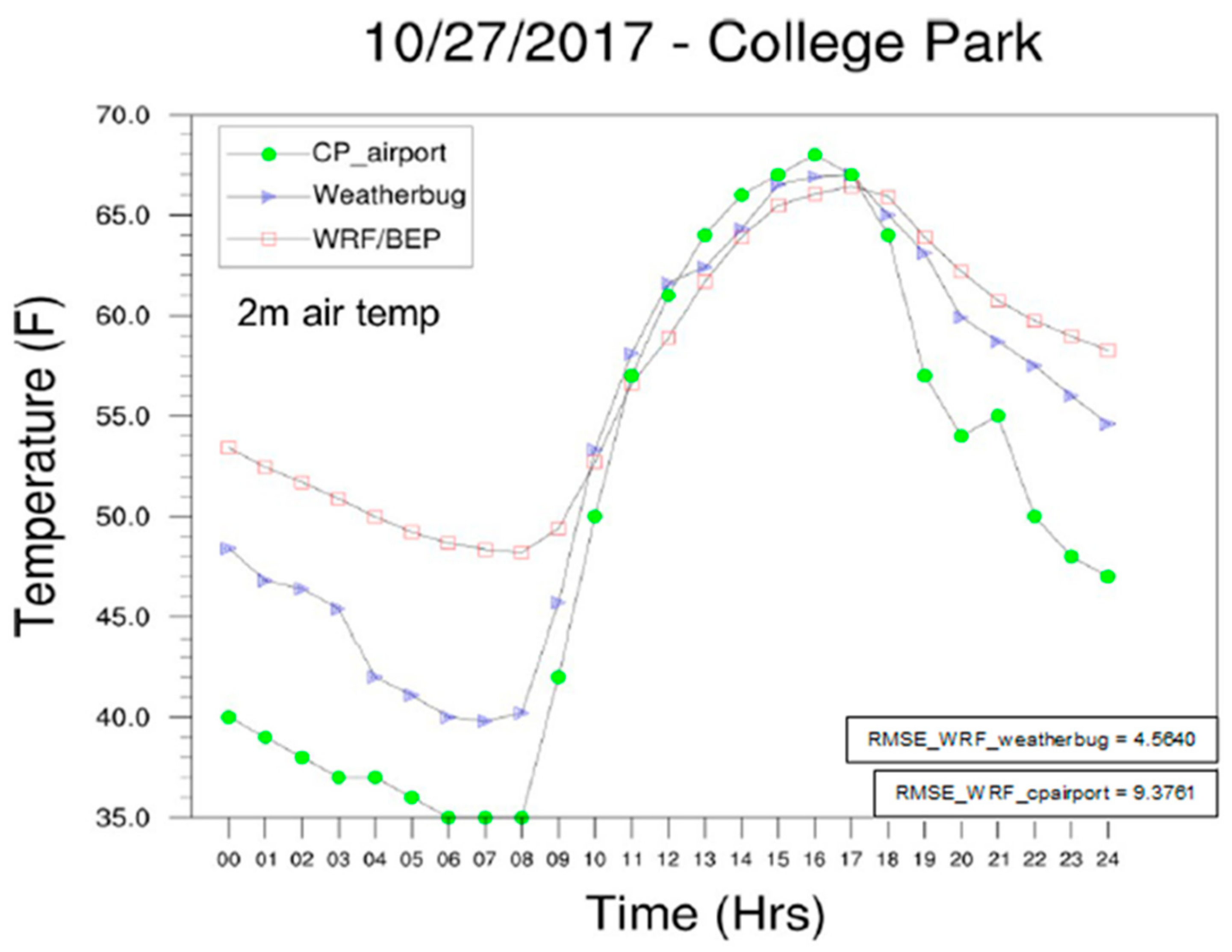
The most significant flaw observed in the default BEP-implemented WRF runs (WRF/BEP) is overestimation of UHI at night. For example, one clear day (10/27/2017) was randomly chosen to demonstrate the deficiencies in the BEP scheme (Figure 1). Evidently, there is an agreement in the BEP surface (two-meter) air temperature with the observations during the daytime. However, the model significantly overestimates the night temperature, with a maximum difference up to 9 °F in the early morning. This is at least partly because anthropogenic UHI mechanisms are absent from the BEP model. The campus buildings hold excess heat and re-emit longwave energy to heat up the surrounding air during the night, as the result of the temperature gradient between the urban canopy and the surrounding rural regions. However, the modeled two-meter air temperature is much higher than those observed at night, indicating an overestimation of the UHI effect in model. Note that the RMS error (RMSE) of WRF/BEP-simulated two-meter air temperature is as high as 4.56 °F when compared with WeatherBug observation and is 9.38 °F when compared with the College Park airport observations, partly because WRF/BEP simulates campus conditions, which is an urban setting and thus the model output is close to the urban observations. In addition, RMS is a statistical index to accumulate all errors at each hour during the daily simulation. The daily averaged difference between model simulation and WeatherBug data is about 2.13 °F.
For a small urban region like College Park, MD, the UHI is still evident. Specifically, at night, the WeatherBug-based temperature is about 5 °F higher than the airport-based temperature, which is only two miles away from the campus but in a rural setting, whereas the WeatherBug site is located on the campus, an urban setting.
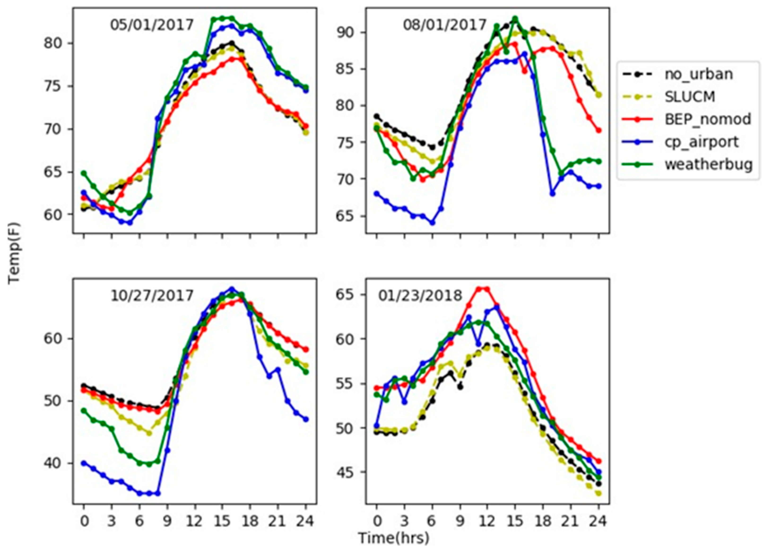
Default WRF models, “no_urban” scheme, SLCUM”, and “BEP_nomod”, show obvious deficiencies in two-meter air temperature simulations when compared with the local WeatherBug temperature which is on a campus building roof and with the College Park airport observations (Figure 2). First of all, four randomly selected days were used to represent spring, summer, fall, and winter, respectively. Again, UHI is evident at night since the building is hotter than the airport (i.e., “cp_airport” vs. “weatherbug”) in May, August, and October by up to 10 °F (e.g., 08/01/2017). The winter day (01/23/2018) UHI is not evident because this day is a cloudy day. Second, although Bep_nomod is better than the no-urban and SLUCM cases, it still largely differs from the observations. The black, yellow, and red line curves show that for each of the days, the diurnal variation represented by the BEP scheme generally better, although SLUCM performs better than the other two schemes for the case of 10/27/2017. Nevertheless, all these three default models simulate UHI with large deficiencies; in particular, in late afternoon or early morning with some overestimating (e.g., nighttime of 05/01/2017, 10/27/2017) and underestimating UHI (e.g., afternoon of 05/01/2017).
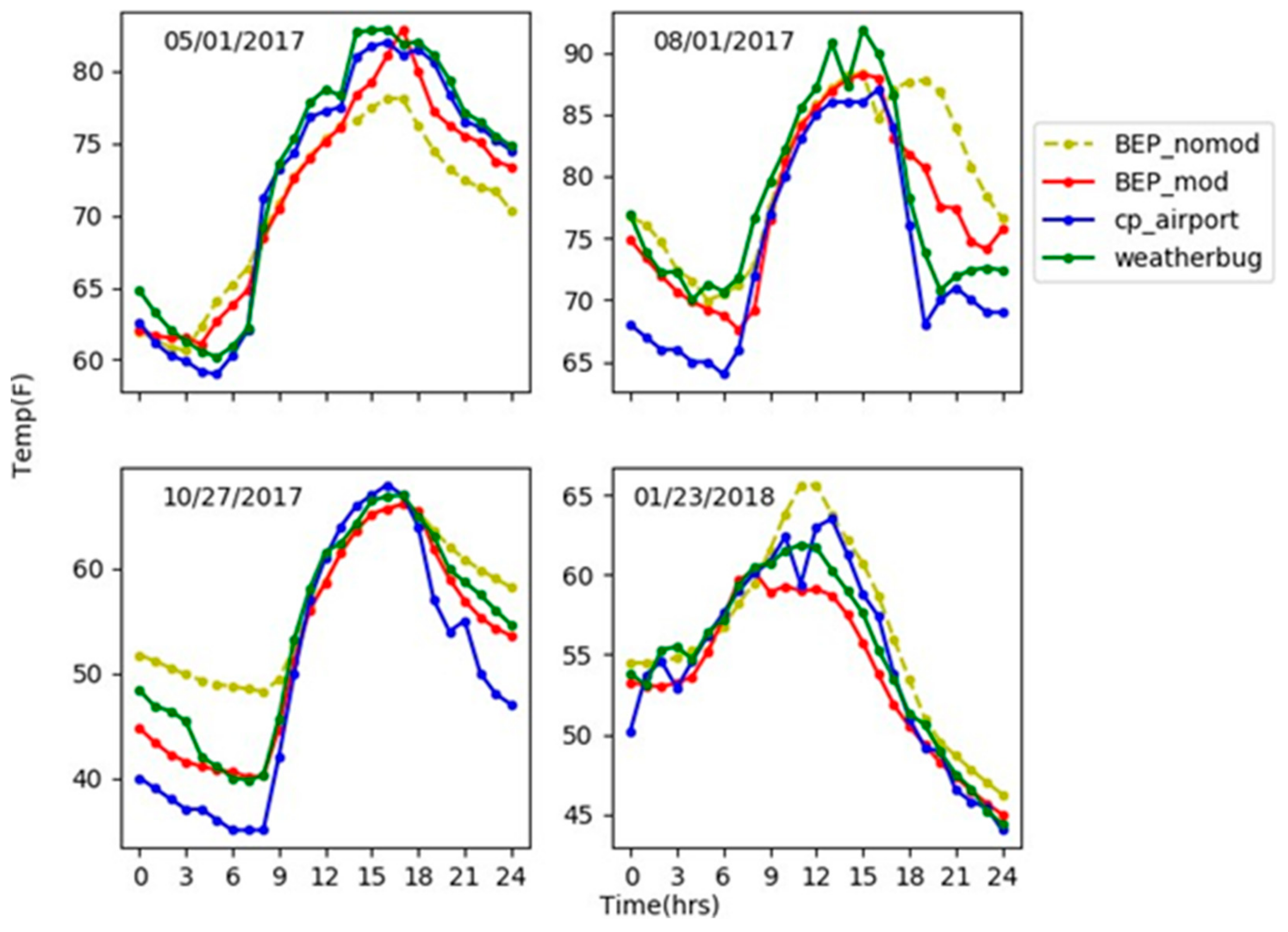
After the modifications of anthropogenic heat flux, the BEP model (“BEP_mod”) performed better than the original BEP_nomod (Figure 3). BEP_mod is close to the observations in both the daytime at the nighttime. In particular, on 08/01/2017, the improved BEP_mod is more accurate at late afternoon and early evening, with the difference at 6 p.m. changing from a previous 17 °F (Figure 2) to 7 °F. Such an improvement suggests that the modifications of heat flux effectively enhance the model’s performance. In addition, significant improvements also occurred on 10/27/2017, with nighttime two-meter air temperatures now close to the WeatherBug observations. This may suggest that the heat flux modification is most effective for high solar radiation days; for example, Summer to Fall seasons and on clear days.
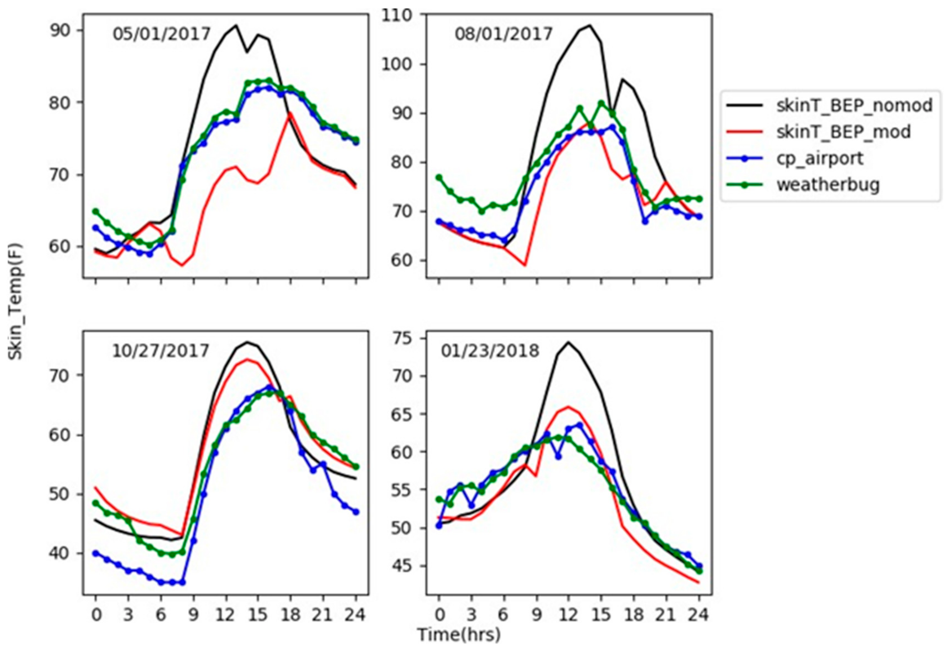
Skin temperature is a parameter closely related to two-meter air temperature but has different physical meaning and magnitude [11]. Nevertheless, unlike two-meter air temperatures, skin temperature observations are not regularly available. Therefore, simulating skin temperature is of great importance. BEP_mod-simulated skin temperatures are most accurate in August, October, and January (Figure 4), with skin temperature higher than two-meter air temperature during daytime and lower than two-meter air temperature at night, which is a typical pattern that has been previously observed [11]. On 05/01/2017, skin temperature simulated by BEP_mod is underestimated, suggesting a possible overcorrection during the daytime and thus further improvement is needed.
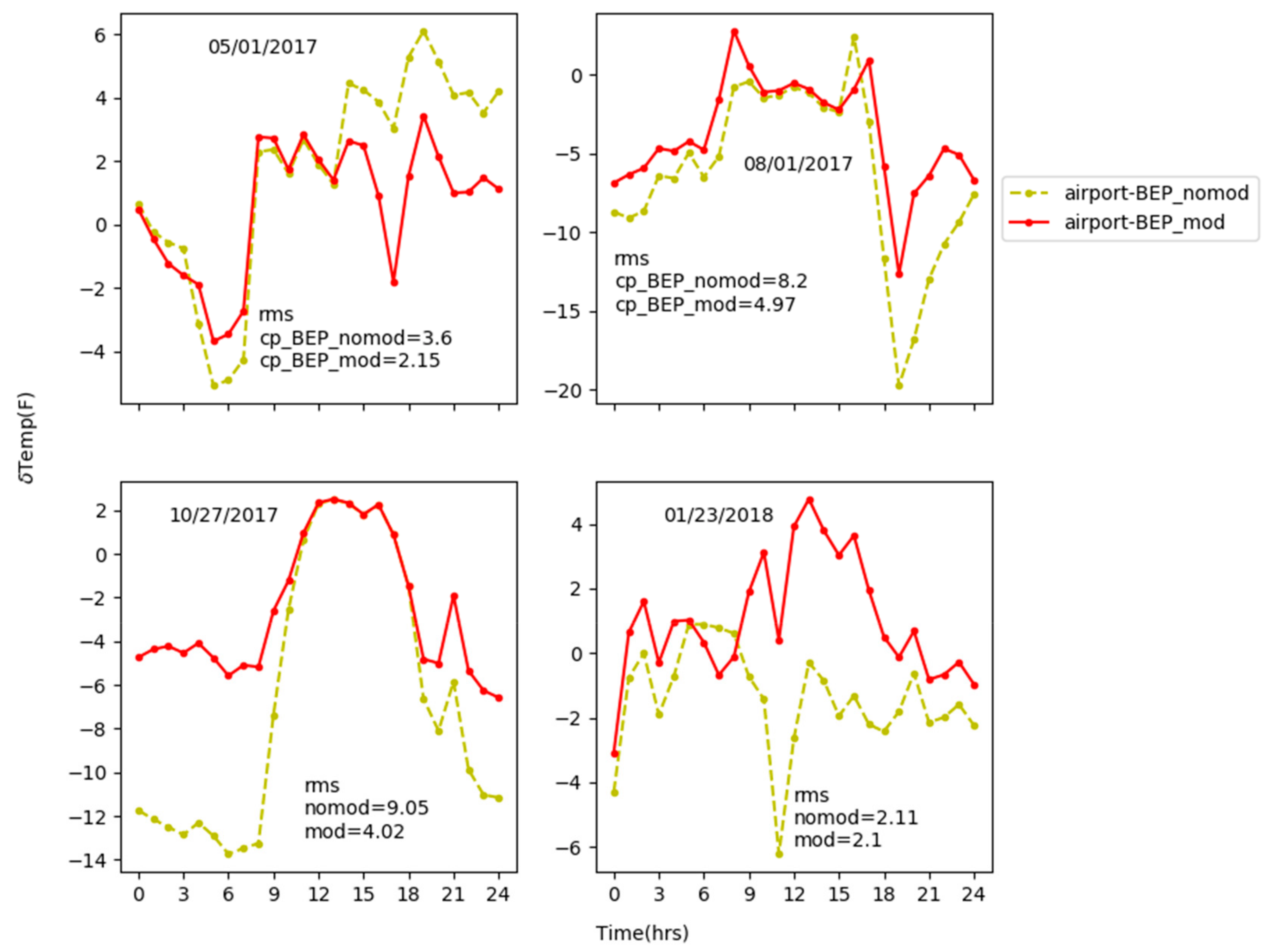
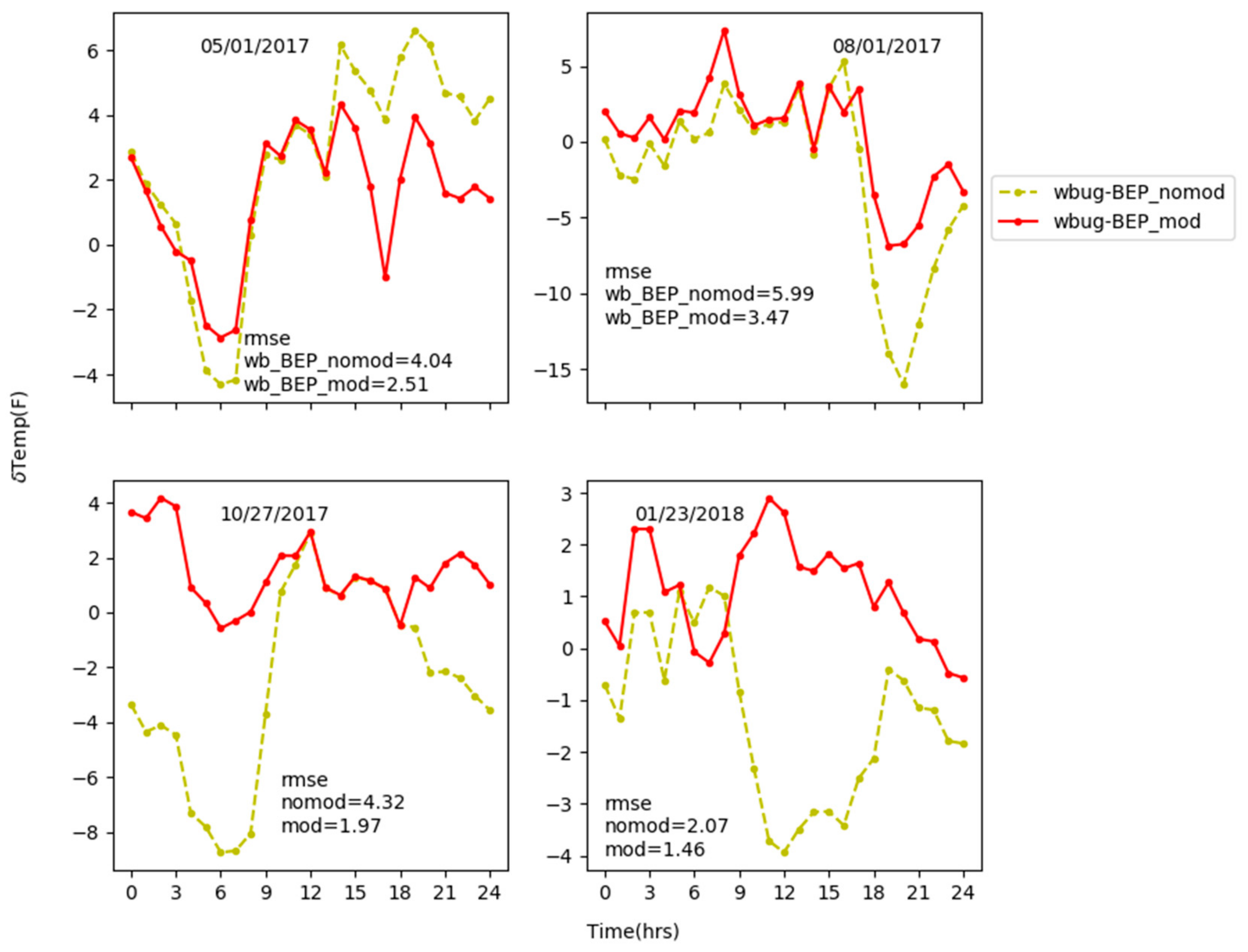
To quantify the improvement in model performance, the root mean square (RMS) error between the modeled temperature and the observation was calculated for each of the four days of the “ nomod” and “ mod” BEP temperatures against the WeatherBug (Figure 5) and College Park airport (Figure 6) observations, respectively. The errors in the modeled temperature with respect to the WeatherBug observations were generally smaller than those with respect to the College Park airport observations, simply because the model is set to simulate an urban setting. The airport observations are made in an area that is limited in terms of characteristic urban features, whereas the WeatherBug sensor records observations in a region that qualifies as a typical urban canopy. Regarding daily average, a 0.5–2.5 °F improvement occurred for the four different season days; for example, 5.99 °F vs. 3.47 °F for 08/01/2017. Although 3.47 °F is still a relatively large error, it is an improvement.
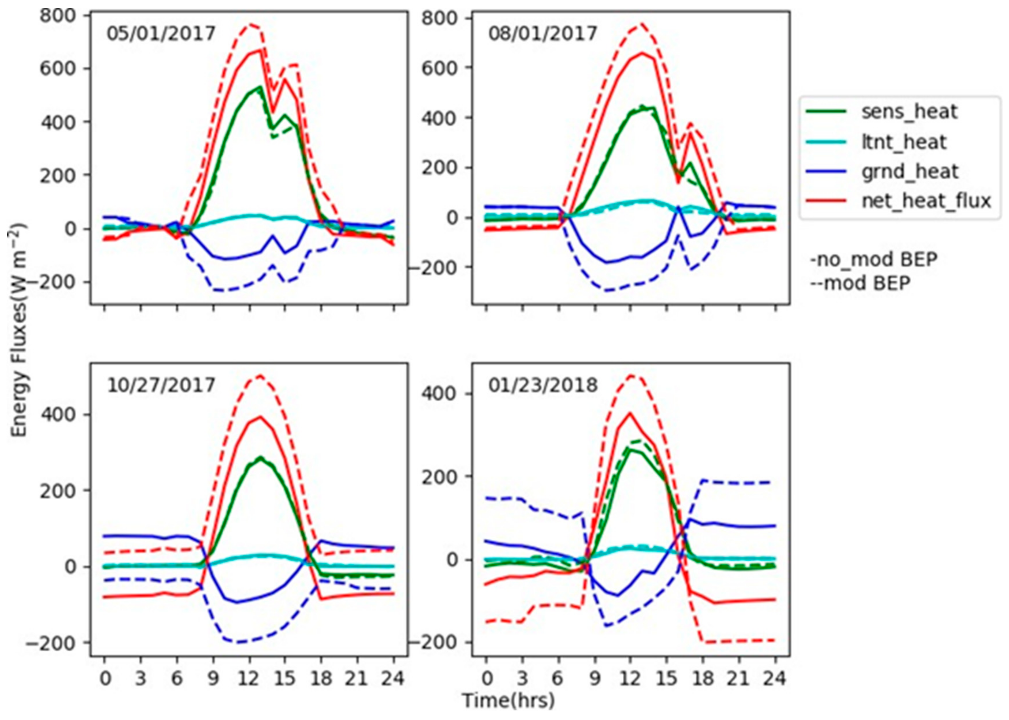
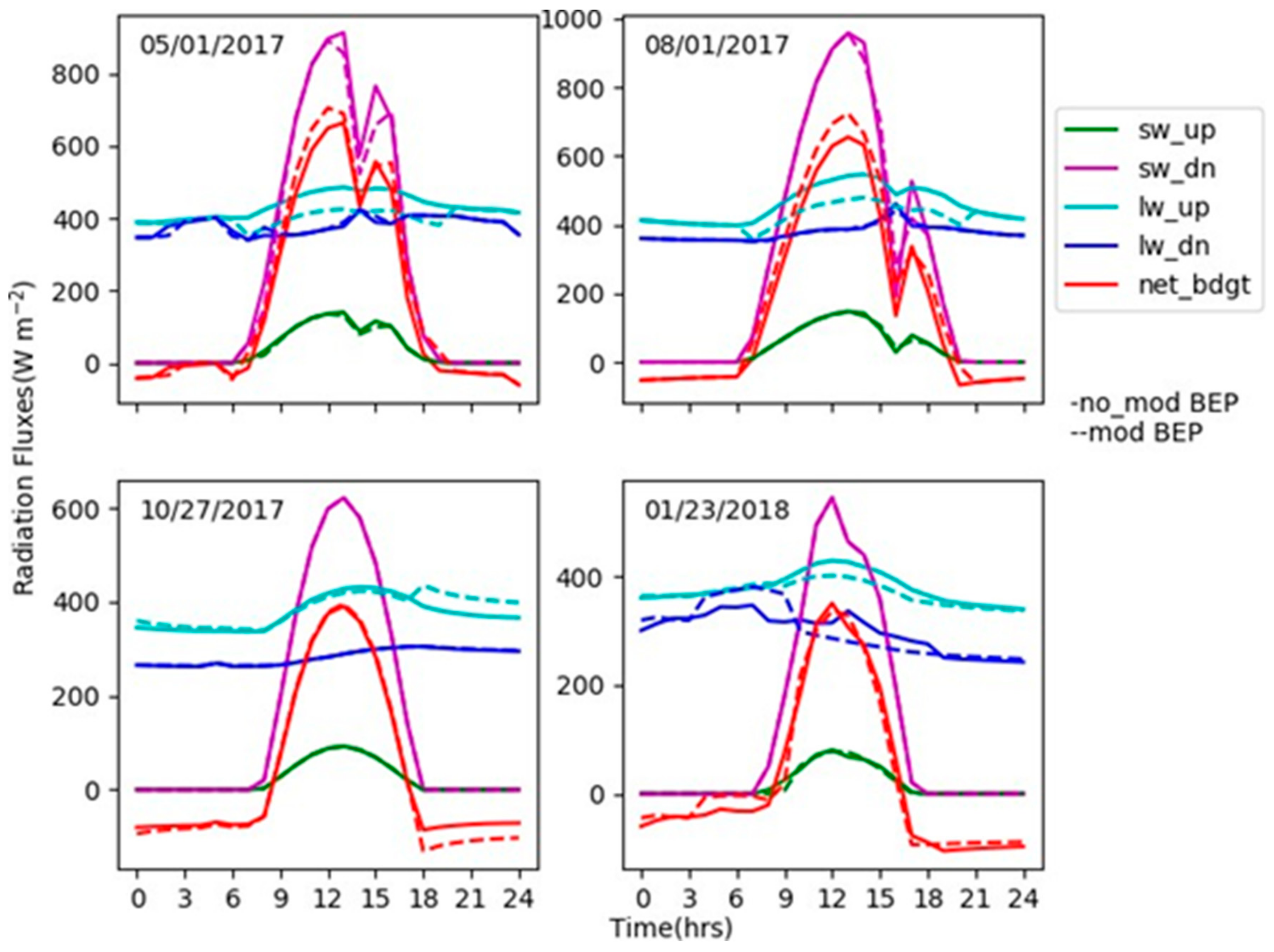
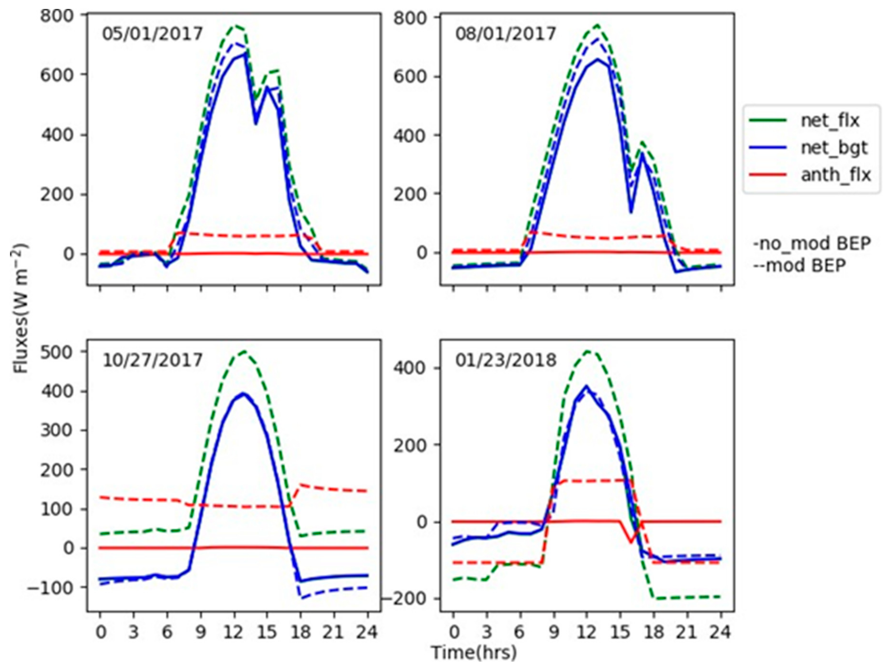
The correction of the net ground flux is higher than that of the other flux components (Figure 7). The skin temperature depends on the net heat transport over the ground, and is thus significantly modified after adding an adequate amount of anthropogenic heating into the heat flux equation. At noon, the ground heat flux is now as high as 200 Wm-2, as shown in Figure 7, for the four different season days. In addition, radiation terms, as presented in Figure 8, show the distribution of radiation budget. For example, upward solar radiation is determined by day surface albedo and thus remains the same for both the original BEP_nomod and BEP_mod models. Nevertheless, the net radiation budgets show the largest difference in May and August with peaks at noon. The fluxes obtained for both of the cases from the radiation budget equation are almost identical to each other. This is because there have been no significant alterations done to the shortwave and longwave radiation over the surface. However, the bias between the net heat flux (obtained from summing up the sensible, latent, and ground heat fluxes) is clearly visible. For the “nomod” case, the net heat flux directly balances out the flux obtained from the budget equation, assuming incorrectly modeled anthropogenic flux. The estimates of the skin and surface air temperatures are hence inaccurate. The deviation observed for the “mod” cases is compensated by the corrected anthropogenic flux, which is shown in Figure 9. In the default BEP run, the “anthropogenic” flux term is consistently close to 0 (Figure 9). Hence, it can be inferred that the rectification in the surface air and skin temperatures observed after correcting the governing equation is due to the addition of the anthropogenic flux term to the equation. After the correction, the diurnal cycle of anthropogenic heat flux is clearly observed for all four days.
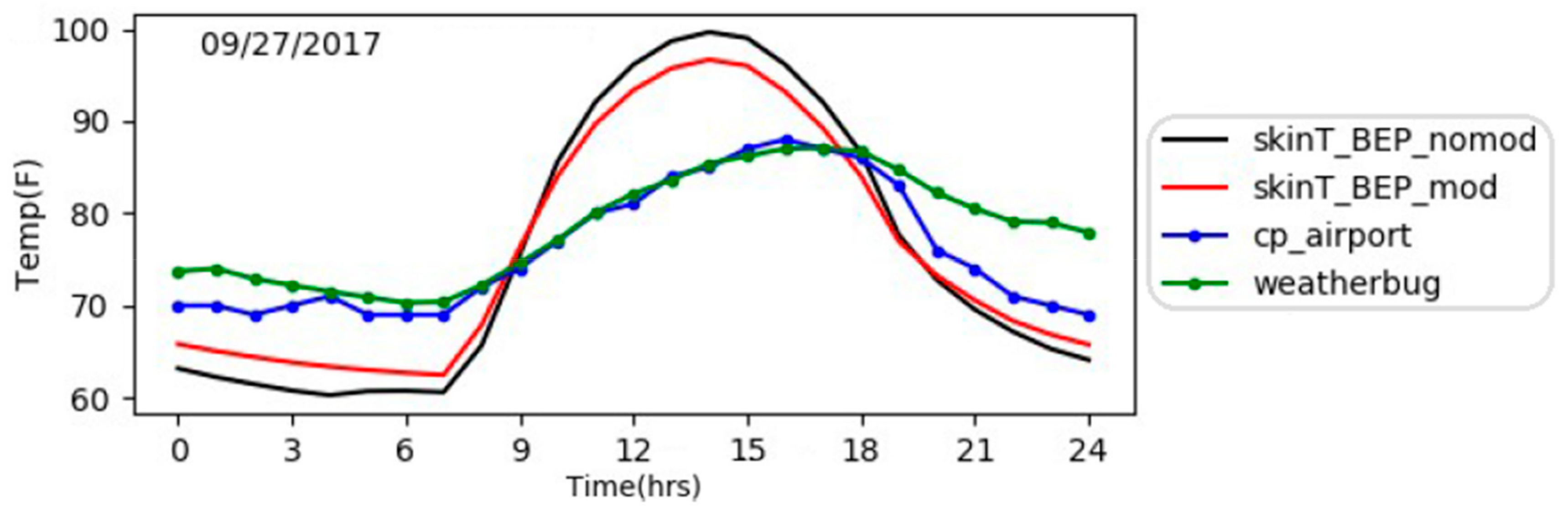
In order to assess model performance on cloudy days, one overcast day (09/27/2017) was analyzed (Figure 10). On cloudy days, UHI is not evident during the daytime compared to the airport temperature and WeatherBug® observations. The daytime temperature at these two regions are very close. Nevertheless, at night, UHI still is evident with about 5 °F at 9 p.m., due partly to the anthropogenic heat flux induced by traffic and buildings.
5. Conclusions
This study enhances the understanding of how well the BEP simulates surface temperature in a small city for various seasons and for clear and clouds days. When compared with the observed two-meter air temperatures, the original BEP urban scheme systemically simulates this variable incorrectly at nights by sometimes overestimating and other times underestimating it by about 5 °F. This indicates a needs for improvement, not only of the temperature scheme but probably also of solar radiation simulation in the atmosphere model or soil moisture in the hydrological scheme. The broad impact of this is that the enhanced scheme may help to better simulate regional climate change and produce gridded information for further use in impact assessments.
One anthropogenic heat flux mechanism is missing in BEP model design and we added this into the original BEP model framework. This simple modification evidently improved the UHI simulations for all seasons. Skin temperature and two-meter air temperature were more accurately modeled after adding the anticipatory anthropogenic heating term to the ground heat flux in the governing budget equation. Nevertheless, anthropogenic heat flux seems to be a function of city size, road conditions, population, and traffic density. Thus, the equation given in the study should only serve as an example. For other cities, this term may have different magnitude. Furthermore, other physical processes of surface energy budget in the BEP model need to be investigated once anthropogenic heat flux is added.
This work was conducted on a university campus, which is covered by roads, buildings, and parking lots. However, its urban features are not as intense as those of an urban canyon and thus the BEP model, which is designed for urban canyon characteristics, may be too complex and thus underperform over such a small urban domain. The first set of sensitivity runs (involving the implementation of SLUCM) carried out over the College Park area delivered slightly better set temperature values. The SLUCM enables the incorporation of the urban framework in a very fundamental manner, with the assumption of invariant building height and uniform material composition.
The BEP is a multilevel urban scheme assuming a complicated urban setting. The variable building height and the segregation in terms of the areas constituting the roads, building roofs, and building walls, which are considered changes in the roughness length, help in capturing the details of the heat transport better than in the control run and the sensitivity run conducted with SLUCM. The initial results corresponding to the BEP scheme are inaccurate because of the underestimation of the ground heat fluxes and overestimation of the incoming shortwave radiation. The lack of heat loss through ground fluxes at night results in marginally higher values of two-meter air temperature mainly during the nighttime. After making adjustments in the ground flux (to incorporate the anthropogenic flux), the two-meter air temperature simulations improved substantially. The heat fluxes and the overall diurnal budget endorse the changes related to anthropogenic heat flux.
Author Contributions
M.S.J. proposed and conceived the idea of this research. K.G. worked on data acquisition and performed WRF runs to obtain forecasts for performing analyses. M.S.J. and K.G. did the analysis of the forecast results obtained via WRF runs. This task of finishing the paper was done by M.S.J.
Funding
This research received funding support from Maryland Innovation Initiative (MII).
Conflicts of Interest
The authors declare no conflict of interest.
References
- Chehbouni, A.; Seen, D.L.; Njoku, E.; Lhomme, J.-P.; Monteny, B.; Kerr, Y. Estimation of sensible heat flux over sparsely vegetated surfaces. J. Hydrol. 1997, 188, 855–868. [Google Scholar] [CrossRef]
- Rizwan, A.M.; Dennis, L.Y.; Chunho, L.I.U. A review on the generation, determination and mitigation of Urban Heat Island. J. Environ. Sci. 2008, 20, 120–128. [Google Scholar] [CrossRef]
- Jin, M.; Dickinson, R.E.; Zhang, D. The footprint of urban areas on global climate as characterized by MODIS. J. Clim. 2005, 18, 1551–1565. [Google Scholar] [CrossRef]
- Zhang, N.; Wang, X.; Peng, Z. Large-eddy simulation of mesoscale circulations forced by inhomogeneous urban heat island. Bound.-Layer Meteorol. 2014, 151, 179–194. [Google Scholar] [CrossRef]
- Ichinose, T.; Shimodozono, K.; Hanaki, K. Impact of anthropogenic heat on urban climate in Tokyo. Atmos. Environ. 1999, 33, 3897–3909. [Google Scholar] [CrossRef]
- Offerle, B.; Grimmond, C.S.B.; Fortuniak, K. Heat storage and anthropogenic heat flux in relation to the energy balance of a central European city centre. Int. J. Climatol. 2005, 25, 1405–1419. [Google Scholar] [CrossRef]
- Offerle, B.; Eliasson, I.; Grimmond, C.S.B.; Holmer, B. Surface heating in relation to air temperature, wind and turbulence in an urban street canyon. Bound.-Layer Meteorol. 2007, 122, 273–292. [Google Scholar] [CrossRef]
- Vourlitis, G.L.; Nogueira, J.D.S.; Lobo, F.D.A.; Sendall, K.M.; De Paulo, S.R.; Dias, C.A.A.; Pinto, O.B.; De Andrade, N.L.R. Energy balance and canopy conductance of a tropical semi-deciduous forest of the southern Amazon Basin. Water Resour. Res. 2008, 44, 1–14. [Google Scholar] [CrossRef]
- Moriwaki, R.; Kanda, M. Seasonal and diurnal fluxes of radiation, heat, water vapor, and carbon dioxide over a suburban area. J. Appl. Meteorol. 2004, 43, 1700–1710. [Google Scholar] [CrossRef]
- Jin, M.; Shepherd, J.M. Inclusion of urban landscape in a climate model: How can satellite data help? Bull. Am. Meteorol. Soc. 2005, 86, 681–689. [Google Scholar] [CrossRef]
- Jin, M.; Dickinson, R.E. Land surface skin temperature climatology: Benefitting from the strengths of satellite observations. Environ. Res. Lett. 2010, 5, 044004. [Google Scholar] [CrossRef]
- Myneni, R.B.; Hoffman, S.; Knyazikhin, Y.; Privette, J.L.; Glassy, J.; Tian, Y.; Wang, Y.; Song, X.; Zhang, Y.; Smith, G.R.; et al. Global products of vegetation leaf area and fraction absorbed PAR from year one of MODIS data. Remote Sens. Environ. 2002, 83, 214–231. [Google Scholar] [CrossRef] [Green Version]
- Schaaf, C.B.; Gao, F.; Strahler, A.H.; Lucht, W.; Li, X.; Tsang, T.; Strugnell, N.C.; Zhang, X.; Jin, Y.; Muller, J.P.; et al. First operational BRDF, albedo nadir reflectance products from MODIS. Remote Sens. Environ. 2002, 83, 135–148. [Google Scholar] [CrossRef] [Green Version]
- Salamanca, F.; Georgescu, M.; Mahalov, A.; Moustaoui, M.; Wang, M. Anthropogenic heating of the urban environment due to air conditioning. J. Geophys. Res. Atmos. 2014, 119, 5949–5965. [Google Scholar] [CrossRef]
- Spronken-Smith, R.A.; Oke, T.R. Scale modelling of nocturnal cooling in urban parks. Bound.-Layer Meteorol. 1999, 93, 287–312. [Google Scholar] [CrossRef]
- Kanda, M.; Kawai, T.; Kanega, M.; Moriwaki, R.; Narita, K.; Hagishima, A. A simple energy balance model for regular building arrays. Bound.-Layer Meteorol. 2005, 116, 423–443. [Google Scholar] [CrossRef]
- Grimmond, C.S.B. Progress in measuring and observing the urban atmosphere. Theor. Appl. Climatol. 2006, 84, 3–22. [Google Scholar] [CrossRef]
- Allwine, K.J.; Flaherty, J.E. Joint Urban 2003: Study Overview and Instrument Locations; No. PNNL-15967; Pacific Northwest National Lab. (PNNL): Richland, WA, USA, 2006. [Google Scholar]
- Ren, G.Y.; Chu, Z.Y.; Chen, Z.H.; Ren, Y.Y. Implications of temporal change in urban heat island intensity observed at Beijing and Wuhan stations. Geophys. Res. Lett. 2007, 34. [Google Scholar] [CrossRef]
- Argüeso, D.; Evans, J.P.; Pitman, A.J.; Di Luca, A. Effects of city expansion on heat stress under climate change conditions. PLoS ONE 2015, 10, e0117066. [Google Scholar] [CrossRef]
- Arnfield, A.J. Two decades of urban climate research: A review of turbulence, exchanges of energy and water, and the urban heat island. Int. J. Climatol. 2003, 23, 1–26. [Google Scholar] [CrossRef]
- Zhang, Y.; Murray, A.T.; Turner, B. Optimizing green space locations to reduce daytime and nighttime urban heat island effects in Phoenix, Arizona. Landsc. Urban Plan. 2017, 165, 162–171. [Google Scholar] [CrossRef]
- Beljaars, A.C.M.; Holtslag, A.A.M. Flux parameterization over land surfaces for atmospheric models. J. Appl. Meteorol. 1991, 30, 327–341. [Google Scholar] [CrossRef]
- Henderson-Sellers, B. Calculating the surface energy balance for lake and reservoir modeling: A review. Rev. Geophys. 1986, 24, 625–649. [Google Scholar] [CrossRef]
- Garratt, J.R.; Pielke, R.A. On the sensitivity of mesoscale models to surface-layer parameterization constants. Bound.-Layer Meteorol. 1989, 48, 377–387. [Google Scholar] [CrossRef]
- Sun, J.; Mahrt, L. Determination of surface fluxes from the surface radiative temperature. J. Atmos. Sci. 1995, 52, 1096–1106. [Google Scholar] [CrossRef]
- Zhang, H.; Jin, M.S.; Leach, M. A study of the oklahoma city urban heat island effect using a wrf/single-layer urban canopy model, a joint urban 2003 field campaign, and modis satellite observations. Climate 2017, 5, 72. [Google Scholar] [CrossRef]
- Changnon, S.A., Jr. Urban effects on severe local storms at St. Louis. J. Appl. Meteorol. 1978, 17, 578–586. [Google Scholar] [CrossRef]
- Oke, T.R. The energetic basis of the urban heat island. Q. J. R. Meteorol. Soc. 1982, 108, 1–24. [Google Scholar] [CrossRef]
- Kug, J.-S.; Ahn, M.-S. Impact of urbanization on recent temperature and precipitation trends in the Korean peninsula. Asia-Pac. J. Atmos. Sci. 2013, 49, 151–159. [Google Scholar] [CrossRef]
- Akbari, H.; Cartalis, C.; Kolokotsa, D.; Muscio, A.; Pisello, A.L.; Rossi, F.; Santamouris, M.; Synnefa, A.; Wong, N.H.; Zinzi, M. Local climate change and urban heat island mitigation techniques–The state of the art. J. Civ. Eng. Manag. 2016, 22, 1–16. [Google Scholar] [CrossRef]
- Wong, L.P.; Alias, H.; Aghamohammadi, N.; Aghazadeh, S.; Sulaiman, N.M.N. Urban heat island experience, control measures and health impact: A survey among working community in the city of Kuala Lumpur. Sustain. Cities Soc. 2017, 35, 660–668. [Google Scholar] [CrossRef]
- Kondo, H.; Genchi, Y.; Kikegawa, Y.; Ohashi, Y.; Yoshikado, H.; Komiyama, H. Development of a multi-layer urban canopy model for the analysis of energy consumption in a big city: Structure of the urban canopy model and its basic performance. Bound.-Layer Meteorol. 2005, 116, 395–421. [Google Scholar] [CrossRef]
- Martilli, A.; Clappier, A.; Rotach, M.W. An urban surface exchange parameterisation for mesoscale models. Bound.-Layer Meteorol. 2002, 104, 261–304. [Google Scholar] [CrossRef]
- Barlage, M.; Chen, F.; Tewari, M.; Ikeda, K.; Gochis, D.; Dudhia, J.; Rasmussen, R.; Livneh, B.; Ek, M.; Mitchell, K. Noah land surface model modifications to improve snowpack prediction in the Colorado Rocky Mountains. J. Geophys. Res. Atmos. 2010, 115. [Google Scholar] [CrossRef]
- Chen, F.; Kusaka, H.; Bornstein, R.; Ching, J.; Grimmond, C.S.B.; Grossman-Clarke, S.; Loridan, T.; Manning, K.W.; Martilli, A.; Miao, S.; et al. The integrated WRF/urban modelling system: development, evaluation, and applications to urban environmental problems. Int. J. Climatol. 2011, 31, 273–288. [Google Scholar] [CrossRef]
- Oke, T.R. Canyon geometry and the nocturnal urban heat island: comparison of scale model and field observations. J. Climatol. 1981, 1, 237–254. [Google Scholar] [CrossRef]
- Oke, T.R. The urban energy balance. Prog. Phys. Geogr. 1988, 12, 471–508. [Google Scholar] [CrossRef]
- Allen, R.G.; Pereira, L.S.; Raes, D.; Smith, M. Crop Evapotranspiration—Guidelines for Computing Crop Water Requirements-FAO Irrigation and Drainage Paper 56; Food and Agriculture Organization: Rome, Italy, 1998. [Google Scholar]
- Taha, H. Urban climates and heat islands: albedo, evapotranspiration, and anthropogenic heat. Energy Build. 1997, 25, 99–103. [Google Scholar] [CrossRef] [Green Version]
- Fortuniak, K.; Offerle, B.; Grimmond, C.S.B. Grimmond. Application of a slab surface energy balance model to determine surface parameters for urban areas. Lund Electron. Rep. Phys. Geogr. 2005, 5, 90–91. [Google Scholar]
Figure 1.
Two-meter air temperature observed at the WeatherBug site (“Weatherbug”) on one building’s roof of University of Maryland, College Park, College Park airport (“CP_airport”) and original weather research and forecasting (WRF)/building environment parameterization scheme (BEP) model simulation (“WRF/BEP”) for 10/27/2017.

Figure 2.
Comparisons of WRF land model-simulated two-meter air temperature with College Park airport and WeatherBug observations. The models are the WRF/Noah default model without urban scheme (“no_urban”), the WRF/SLUCM model (“SLUCM”), and the original WRF/BEP model (“BEP_nomod”). Four different days were selected to represent different seasons.

Figure 3.
Comparison of two-meter air temperatures simulated by the original BEP (“BEP_nomod”) and improved BEP (“BEP_mod”) for the College Park airport and campus building WeatherBug sites for four different days in College Park, MD.
Figure 3.
Comparison of two-meter air temperatures simulated by the original BEP (“BEP_nomod”) and improved BEP (“BEP_mod”) for the College Park airport and campus building WeatherBug sites for four different days in College Park, MD.

Figure 4.
Comparison of two-meter air temperatures simulated by the original BEP (“BEP_nomod”) and improved BEP (“BEP_mod”) for the College Park airport and campus building WeatherBug sites for four different days in College Park, MD.
Figure 4.
Comparison of two-meter air temperatures simulated by the original BEP (“BEP_nomod”) and improved BEP (“BEP_mod”) for the College Park airport and campus building WeatherBug sites for four different days in College Park, MD.

Figure 5.
RMS error calculation between the modeled surface air temperature and the observations of the WeatherBug site.
Figure 5.
RMS error calculation between the modeled surface air temperature and the observations of the WeatherBug site.

Figure 6.
RMS error calculation between the modeled surface air temperature and the observations of the College Park airport site.
Figure 6.
RMS error calculation between the modeled surface air temperature and the observations of the College Park airport site.

Figure 7.
Heat fluxes and net fluxes computed from the energy budget for four days. The unit is Wm−2.
Figure 7.
Heat fluxes and net fluxes computed from the energy budget for four days. The unit is Wm−2.

Figure 8.
Radiative energy terms in the original BEP model (solid line) and the modified BEP model (dashed line). Unit is Wm−2.
Figure 8.
Radiative energy terms in the original BEP model (solid line) and the modified BEP model (dashed line). Unit is Wm−2.

Figure 9.
Net heat fluxes (“net_flx”), net radiative energy (“net_bgt”), and anthropogenic flux (“anth_flx” for the original WRF/BEP model (“nomod”) and the modified WRF/BEP model (“ mod”) simulations. Unit is Wm−2.
Figure 9.
Net heat fluxes (“net_flx”), net radiative energy (“net_bgt”), and anthropogenic flux (“anth_flx” for the original WRF/BEP model (“nomod”) and the modified WRF/BEP model (“ mod”) simulations. Unit is Wm−2.

Figure 10.
Skin temperature simulations and measurements for one overcast day. The unit is °F.

© 2019 by the authors. Licensee MDPI, Basel, Switzerland. This article is an open access article distributed under the terms and conditions of the Creative Commons Attribution (CC BY) license (http://creativecommons.org/licenses/by/4.0/).
Share and Cite
MDPI and ACS Style
Gohil, K.; Jin, M.S. Validation and Improvement of the WRF Building Environment Parametrization (BEP) Urban Scheme. Climate 2019, 7, 109. https://0-doi-org.brum.beds.ac.uk/10.3390/cli7090109
AMA Style
Gohil K, Jin MS. Validation and Improvement of the WRF Building Environment Parametrization (BEP) Urban Scheme. Climate. 2019; 7(9):109. https://0-doi-org.brum.beds.ac.uk/10.3390/cli7090109
Chicago/Turabian StyleGohil, Kanishk, and Menglin S. Jin. 2019. "Validation and Improvement of the WRF Building Environment Parametrization (BEP) Urban Scheme" Climate 7, no. 9: 109. https://0-doi-org.brum.beds.ac.uk/10.3390/cli7090109
Note that from the first issue of 2016, this journal uses article numbers instead of page numbers. See further details here.