Article

Spatial Process of Surface Urban Heat Island in Rapidly Growing Seoul Metropolitan Area for Sustainable Urban Planning Using Landsat Data (1996–2017)

by
Prabath Priyankara
1,2,*,
Manjula Ranagalage
3,4,
DMSLB Dissanayake
1,4,
Takehiro Morimoto
3 and
Yuji Murayama
3
1
Graduate School of Life and Environmental Sciences, University of Tsukuba, 1-1-1, Tennodai, Tsukuba, Ibaraki 305-8572, Japan
2
Faculty of Agriculture, University of Ruhuna, Mapalana, Kamburupitiya 81100, Sri Lanka
3
Faculty of Life and Environmental Sciences, University of Tsukuba, 1-1-1, Tennodai, Tsukuba, Ibaraki 305-8572, Japan
4
Department of Environmental Management, Faculty of Social Sciences and Humanities, Rajarata University of Sri Lanka, Mihintale 50300, Sri Lanka
*
Author to whom correspondence should be addressed.
Submission received: 2 August 2019 / Revised: 30 August 2019 / Accepted: 8 September 2019 / Published: 11 September 2019
(This article belongs to the Special Issue Urban Heat Islands)

Abstract

:
The urban heat island (UHI) phenomenon is an important research topic in the scholarly community. There are only few research studies related to the UHI in the Seoul metropolitan area (SMA). Therefore, this study examined the impact of urbanization on the formation of UHI in the SMA as a geospatial study by using Landsat data from 1996, 2006, and 2017. For this purpose, we analyzed the relative variation of land surface temperature (LST) with changes of land use/land cover (LULC) rather than absolute values of LST using gradient, intensity, and directional analyses. It was observed that the impervious surface (IS) has expanded, and the UHI effect was more penetrating in the study area, with considerable loss of other LULC including green surfaces along with the rapid urbanization of the study area. In this study, we divided the IS into persistent IS (PIS) and newly added IS (NAIS). The spatial distribution of the IS, forest surface (FS), PIS, and NAIS was observed based on gradient zones (GZs). The results show that GZ1 recorded a difference of 6.0 °C when compared with the GZ109 in 2017. The results also show that the city center was warmer than the surrounding areas during the period of study. Results reveal that the mean LST has a strong significant positive relationship with a fraction of IS and PIS in 2006 and 2017. On other hand, the mean LST has a strong negative relationship with a fraction of FS and NAIS in the same time points. Relatively low temperatures were recorded in FS and NAIS in both time points. Further, it was proved that the local climate of the SMA and its surroundings had been affected by the UHI effect. Therefore, urban planners of the SMA should seriously consider the issue and plan to mitigate the effect by improving the green surfaces of the city. More greening-oriented concepts are recommended in both horizontal and vertical directions of the SMA, that can be used to control the negative impact associated with UHI. The overall outputs of the study could be used as a proxy indicator for the sustainability of the SMA and its surroundings.

Graphical Abstract

1. Introduction

Currently, 55% of the world’s total population (7.7 billion) is accommodated in urban areas, a proportion that is expected to increase up to 68% in 2050 [1]. Urbanization is the process of a gradual residential shift of the human population from rural to urban areas. Projections show that 2.5 billion more people will be added to cities and surrounding areas by 2050, in parallel with the overall growth of the world’s population. Interestingly, 90% of this will take place in Asia and Africa [1]. The current level of urbanization in Asia is now approximated to be 50% [1]. This rapid urban development resulted in converting different land uses and land covers, like vegetation and open land, into impervious surfaces (IS) [2].
Land use/land cover (LULC) encompasses a set of human-made and natural components and their spatial distributions [3]. In the daytime, IS absorbs some amount of solar radiation, the rest is reflected, and reradiates the absorbed heat in the night-time [3,4]. As a result of these two phenomena, urban areas are globally warmer in comparison with the surrounding areas. Cities with a population of one million or more have a 1–3 °C recorded temperature difference with the surrounding rural areas in the daytime, and it can be as high as 12 °C, especially in the night-time [5].
On the other hand, green surfaces tend to both absorb and reflect solar radiation and, with evapotranspiration, add moisture to the atmosphere that tends to decrease land-surface temperature (LST) [6]. The occurrence of higher air and surface temperatures existing in urban areas than suburban and rural areas is known as the urban heat island (UHI) phenomenon [7,8]. There are two types of UHI: (i) surface UHI (SUHI), which is based on LST, and (ii) atmospheric UHI, which is based on air temperature [8]. The effect of SUHI exists both during the day and night, but its intensity in the daytime is high because of radiation from the sun [8]. With the advancement of sensor technology, thermal remote observation for measuring SUHI became more popular with the use of satellite platforms such as Landsat with larger area of coverage (global coverage) and availability of temporal datasets. Also, with satellite data it is possible to measure energy consumptions of buildings as well. While, atmospheric UHI studies are totally based on data collected from weather stations and having limitations such as unavailability of precious temporal datasets, unavailability of data in some areas, and issues on generalizing temperature data using interpolation techniques [9]. Therefore, studies on surface UHI is more a popular and timely task. Hence, in this study we considered the effect of daytime SUHI.
Urbanization brings numerous socioeconomic benefits to urban populations, but it also brings some adverse effects to the natural environment [10,11]. SUHI is a one of these tremendous adverse effects of the rapid urbanization process. SUHI has some negative effects such as an increase in energy consumption, adverse effects on the health and comfort of the urban population, and the depression of living conditions [8,12,13]. Therefore, it is crucial to examine the magnitude and trend of the SUHI effect in order to apply proper precautions to minimize it. Due to all these circumstances, studies on SUHI are becoming a substantial research theme among the scholarly community [14,15]. There are several past studies that were conducted to understand the spatial and temporal variation of SUHI magnitude, such as for Baguio City in Philippines [16], Kandy City in Sri Lanka [17,18], Addis Ababa in Ethiopia [3], Lagos in Nigeria, Lusaka in Zambia, Nairobi in Kenya [19], and Tehran in Iran [20]. Still, related studies are needed to enhance the knowledge related to the magnitude of SUHI. Therefore, it is essential to conduct research and analysis on SUHI to address the limitations, which is a significant and timely task.
The spatial and temporal pattern of the magnitude of the SUHI provides valuable information to understand SUHI behavior in urban and surrounding areas. According to Estoque and Murayama (2017) in their study, there were two main methods that have been used to calculate the magnitude of the SUHI: (i) classifying LULC as the local climate zone of the cities and using a crossover comparison [16,18,20,21,22], and (ii) calculating the urban–rural area temperature difference. This can be computed by using urban–rural gradient analysis. Gradient analysis can be employed to recognize the spatial variation of environmental attributes with distance [23]. There are several previous researches that have used gradient analysis to quantify the magnitude of the SUHI [3,16,18,19,24]. In most of the previous researches, mean LST, a fraction of IS, and green surfaces (GS) have been calculated based on gradient analysis. However, all of the previous researches have been made to calculate the temperature difference between IS and GS with two or more time points. But none of the studies were focused on the SUHI differences in IS regarding urbanization process. Therefore, we hypothesized that it was needed to investigate the temperature difference between persistent IS (PIS) and newly added IS (NAIS) to understand the contribution to SUHI formation in urban areas. It is vital to study the impact of PIS, NAIS, and total IS on the effect of SUHI using gradient, intensity, and directional analyses to understand the magnitude and trend of the SUHI effect. This is a useful indicator to evaluate the SUHI effect, as well as the level of environmental friendliness of urban constructions as a different geospatial approach. Thus, in this paper, we separately study PIS and NAIS to provide new research knowledge related to the gradient-based SUHI studies. This is the main difference of this research with the previous researches and it is the originality of the study. In this process, LULC classification plays a significant role.
The recent development of the Geographic Information Systems (GIS) and Remote Sensing (RS) techniques with the use of machine-learning methods in effective and efficient R software-enabled LULC classification allowed us to examine LULC changes in a time-efficient and cost-effective manner compared to conventional methods like ground-based methods [25,26,27]. The use of R software for LULC classification enabled to select the best way from different machine-learning methods with an initial accuracy assessment [28,29,30,31,32]. Extraction of the LST from thermal infrared RS data is also time-efficient and cost-effective, and an alternative to the lack of ground-based temperature data [33]. On the other hand, with thermal RS data, it is possible to achieve a high temporal resolution [34]. Thus, Landsat imagery has been used to classify the LULC and the extraction of LST of the study area.
Megacities located in Southeast Asia have shown considerable urbanization development during the past few decades. SUHI is having a significant adverse impact through the rapid urbanization, and it has negatively influenced environmental quality. The landscape-composition pattern and its relationship with UHI in Bangkok, Jakarta, and Manila were studied by [35] in 2017. They used several methods to understand the behavior of the UHI in three megacities. However, there are few SUHI studies that have been conducted in Seoul [34,36,37,38]. Nearly 80% of the Republic of Korea’s total population (51 million) live in urban areas. According to predictions, the percentage will increase by up to 86% by 2050 [39]. Over one-fifth of the nation’s total population lives in Seoul [40]. Seoul is a highly urbanized megacity, and overpopulation affects LULC changes in Seoul and its immediate surroundings. Urbanization and overpopulation are human activities that alter the landscape of Seoul, which then contributes to the formation of the SUHI phenomenon. Therefore, the goal of the research is to inspect the impact of LULC composition and its relationship with SUHI. Consequently, the specific objectives of this study are as follows: (i) to calculate the landscape composition and its impact on SUHI formation, (ii) to assess the contribution of PIS and NAIS on SUHI formation, and (iii) to calculate multitemporal and multidirectional SUHI profiles. The results of this study are useful for a proxy indicator for sustainable urban planning.

2. Materials and Methods

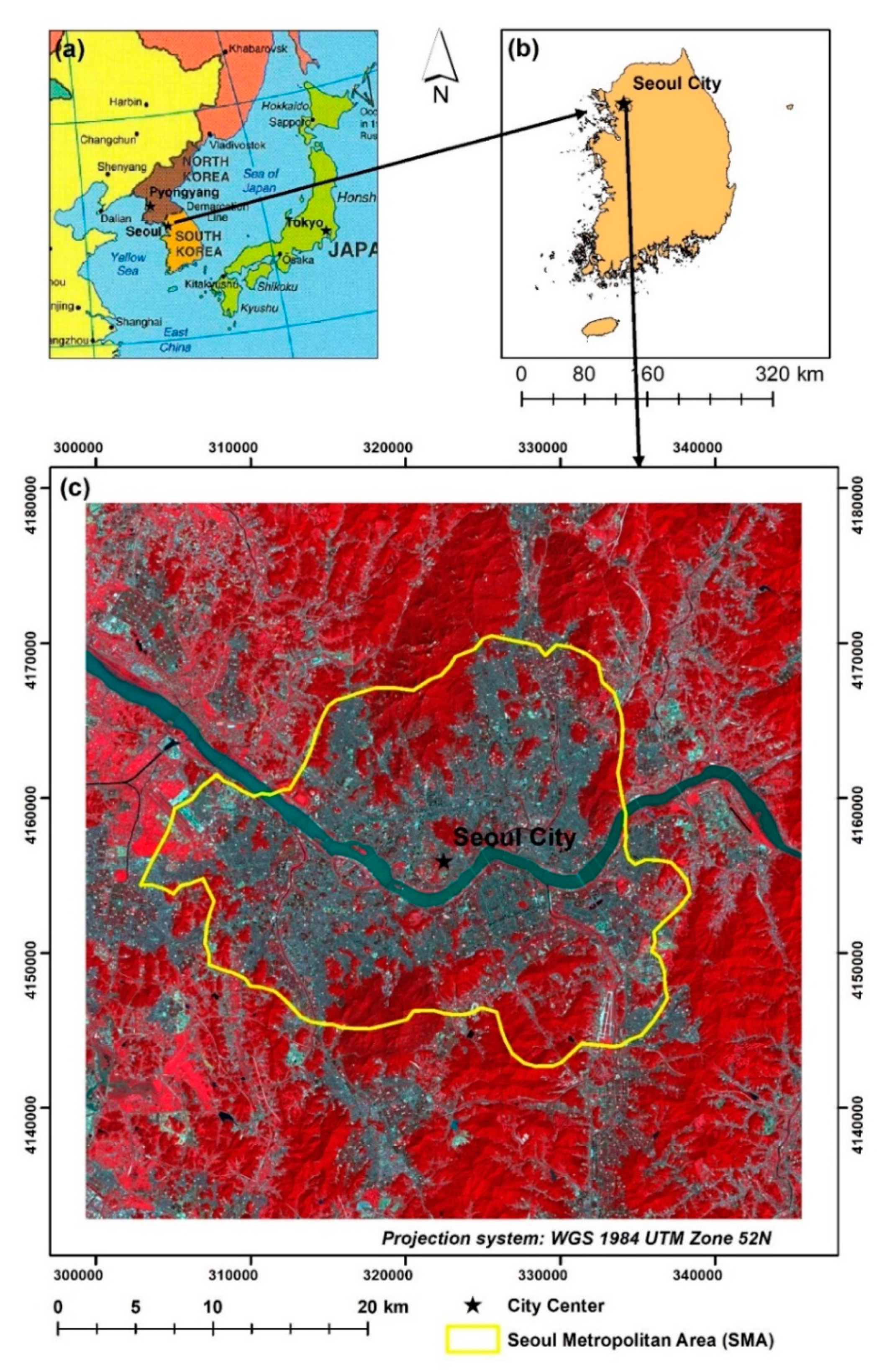
2.1. Study Area: Seoul Metropolitan Area, Republic of Korea

The Seoul metropolitan area (SMA) is the capital and the largest metropolitan area in the Republic of Korea (South Korea) on the Korean Peninsula in the center of Northeast Asia [41]. The geographical setting of SMA extended by northing from 4,170,478.01 to 4,142,707.68 m, and easting from 302,905.38 to 338,355.11 m according to the WGS1984 UTM (52N) projected coordinate system, as shown in Figure 1. The SMA features a humid, continental, and subtropical climate with average annual precipitation of nearly 1450 mm, and more than 60% of precipitation during the summer season (from June to August) because of the influence of East Asian summer monsoon [42]. The mean temperature of the SMA is 24.2 °C in the summer season [42]. The SMA is one of the highly populated cities in the world and around 21.5% (nearly 11 million) of the country’s total population lives in [43]. The geographical mean center of the SMA is defined as the city center with y-coordinate 4,155,930.99 m (northing) and x-coordinate 322,488.87 m (easting).We selected a 46 by 46 km geographical extent as the study area with a 23 km radius from the city center covering 2,116 km2 (Figure 1) of the area, which included the SMA and covered the surrounding characteristics. The geographical setting of the study area extends northing from 4,179,030.95 to 4,132,830.84 m, and easting from 299,388.93 to 345,588.92 m.

2.2. Data Descriptions and Data Preprocessing: Satellite Imagery

Radiometrically calibrated and atmospherically corrected Level 2 on-demand Landsat data were freely collected through the official website of the Geological Survey of the United States (USGS) [46,47]. Band 10 of Landsat-8 Operational Land Imager (OLI)/Thermal Infrared Sensor (TIRS) and Band 6 of Landsat-5 TM were with atmospheric brightness temperature in kelvin (K). All multispectral bands of Landsat-8 OLI/TIRS and Landsat-5 TM were provided as surface-reflectance values [46,47]. For the selection of the satellite images for the study it used the criteria as follows: (i) captured in summer-season; (ii) captured in daytime; and (iii) cloud-free or less-cloud cover (< 10%). With the use of multiple Landsat images for a given time point which leads to generate more accurate results of SUHI effect than just using three images but the limitation due to the cloud cover, it was able to select only one image for a given time point. With the availability of data, 1996 was selected as the base year to find out the SUHI pattern in the developing stage of the country; 2007 was selected to represent the middle stage after the development of the country; and 2017 was selected to represent the present stage of the country. Table 1 shows the comprehensive description of the data used for the study.

2.3. Extraction of Land Use and Land Cover

Four types of machine learning (ML) techniques, namely, support vector machine (SVM), k-nearest neighbor (KNN), random forest (RF), and neural networks (NN), were used for LULC classification [3,28,31,32] of the study area with the use of R software. Both overall accuracy and the kappa statistic were higher (over 90%) with the SVM, and the method was selected for LULC classification of the study area. Three time-point satellite imageries of the research area were classified into four LULC types, namely, forest surface (FS); IS; water bodies (WB); and other lands (OL) as grassland, cropland, and bare land for this study. Post classification rectification was also conducted to enhance the accuracy of the classified LULC maps [48]. The accuracy of each of the classified LULC maps was evaluated by using 500 reference points. The stratified random-sampling techniques was used to generate the reference points [49]. Google Earth and pan-sharpened imageries of the Landsat data generated by applying the Gram–Schmidt spectral-sharpening method [48] were used as a source of reference information for the LULC maps of 2006 and 2017. For the 1996 LULC map, the authors trusted on their visual interpretation of Landsat data with different band combinations [16].

2.4. LST Extraction

Radiometrically calibrated and atmospherically corrected Level 2 Landsat data (as described in Section 2.2.) were used for LST extraction. The thermal bands of Landsat contain at-satellite brightness temperature values in kelvin. The values were scaled by using land-surface emissivity [24,35]. Land-surface emissivity (ε) was derived according to Equation (1) [50] and previous researches also used the same method to calculate emissivity and obtained good results [3,16,18,19,24,51]:
ε = m   P v + n
where ε is land-surface emissivity; m is (εvεs) − (1 − εs) Fεv; n is εs + (1 − εs) Fεv; εs is soil emissivity; εv is vegetation emissivity; F is mean value of shape factor, assuming different geometrical distributions, F=0.55 [50]. Here, we used the finding of [50], m = 0.004, and n = 0.986. Pv is the proportion of vegetation that was computed based on the normalized difference vegetation index (NDVI). Pv was extracted according to Equation (2):
P v = ( ( NDVI NDVI min ) / ( NDVI max   NDVI min ) ) 2
where Pv is the proportion of vegetation; NDVI is the normalized difference vegetation index; NDVImin is the minimum value of NDVI; NDVImax is the maximum value of NDVI. The NDVI is calculated according to Equation (3):
NDVI = ρ N I R ρ R e d ρ N I R + ρ R e d
where NDVI is the normalized difference vegetation index; ρNIR is surface-reflectance values of Band 4 of Landsat-5 TM, and Band 5 of Landsat-8 OLI/TIRS; ρRed is the surface-reflectance values of Band 3 of Landsat-5 TM), and Band 4 of Landsat-8 OLI/TIRS.
Finally, Equation (4) was used to extract the emissivity-corrected LST [24,52]:
LST = T b   / { 1 + ( λ   × T b   ρ ) Ln ε }
where LST is land surface temperature in kelvin; Tb is at-satellite brightness temperature in kelvin; λ is the central-band wavelength of emitted radiance (11.5 μm for Band 6 [24] and 10.8 μm for Band 10 [35]); ρ is h × c/σ (1.438 × 10⁻² m K) where, σ is the Boltzmann constant (1.38 × 10⁻²³ J/K), h is Planck’s constant (6.626 × 10⁻³⁴ J *s), and c is the speed of light (2.998 × 10⁸ m/s), and ε is land-surface emissivity [50]. The resulting LST values in kelvin were converted to degrees Celsius (°C) according to Equation (5).
LST ( ° C ) = LST     273.15
where LST (°C) is the land surface temperature in degrees Celsius; LST is the land-surface temperature in kelvin.

2.5. SUHI Profiling

The surface urban heat island profile was investigated based on the multidirectional SUHI profiles of the study area by following orthogonal and diagonal directions such as east–west, north–south, northwest–southeast, and northeast–southwest. The method was introduced by Estoque and Murayama (2017) in their study. Previous other studies have also used the same method to understand the SUHI profile. The studies were able to generate good results by applying the same method in different regions of the world including East Asia [3,18,51].
To generate the SUHI profile of the study area, the authors were used the following five steps method as introduced by Estoque and Murayama (2017) in their study.
  • Step 1: Located the city center in Seoul called 0 kilometers.
  • Step 2: A set of polygon grids was created by snapping the original LST map of the study area. In this study, we used 210 by 210 m (seven by seven grid) based on previous studies [16,18,51,53].
  • Step 3: The grid where the city center was located was chosen as the center grid (0 grid).
  • Step 4: All other grids in the orthogonal and diagonal directions were created.
  • Step 5: Mean LST, fraction PIS, and NAIS were computed to identify multidirectional and multitemporal SUHI profiles of the study area.

2.6. SUHI Intensity Measurement

SUHI intensity (SUHII) can be calculated based on the LST difference between gradient zones and the LST difference between different LULC categories [16]. In this study, we used two methods to calculate SUHII based on the (i) mean LST difference between gradient zones; and (ii) mean LST difference between different LULC categories such as IS, FS, PIS, and NAIS.
The SUHII along the gradient zones (SUHIIGZ) was calculated based on the 210 m buffer zones from the center grid where the city center was located. Previous studies have also used 210 m buffer zones to calculate the mean LST difference between gradient zones [16,18,51]. Gradient zones (GZs) were generated based on the polygon grid created in Section 2.5. All grids in the same order were dissolved by keeping the center grid as 0. The process resulted in 109 GZs, e.g., GZ1, GZ2, and GZ109. The mean LST, a fraction of IS, FS, PIS, and NAIS, was extracted for each GZ.
SUHII based on the LULC categories (SUHIIIS-FS) was calculated by using the main LULC categories of each year. The main LULC categories, such as IS and FS, and subcategories of IS, namely, PIS and NAIS, were used to calculate the SUHII. First, the mean LST of the each LULC was extracted using zonal statistics available in ArcGIS. Hereafter, mean LST difference was calculated based on the mean LST of each LULC [16,18,51].
The magnitude of SUHIIGZ was calculated based on ∆ mean LST, ∆ fraction of IS, ∆ fraction of FS, ∆ fraction of PIS, and ∆ fraction of NAIS were extracted based on the methodology proposed by Estoque and Murayama [16]. Here, the ∆ mean LST was calculated by subtracting GZs (GZ1 − GZ2 . . . 109). A similar process was used to calculate the ∆ fraction of IS, FS, PIS, and NAIS. Here, GZ1 can be referred to as the gradient zone with the highest fraction of IS at each time point.

3. Results

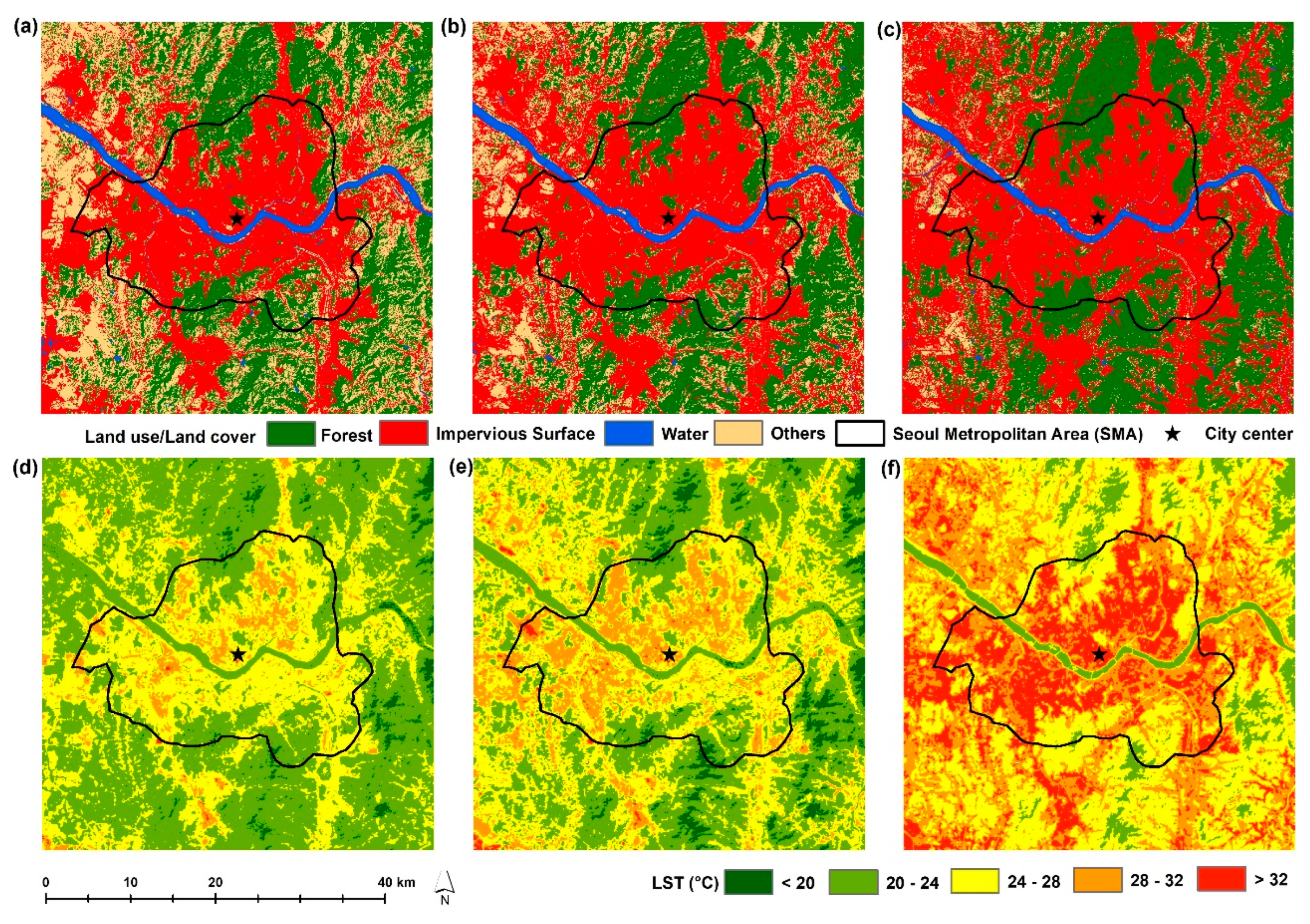
3.1. LULC Changes and LST Distribution

LULC classification was performed according to the methodology explained in Section 2.3. The overall accuracy of the classified LULC maps was 93.2%, 94%, and 94.6% in 1996, 2006, and 2017, respectively. Further, the kappa coefficient was 0.9 in 1996 and 2006, and 0.91 in 2017 (Table 2). The complete error matrix is shown in Table A1, Table A2 and Table A3 in Appendix A. This method was commonly used in similar studies, and its details can be found elsewhere [54]. According to the results of LULC classification, rapid urbanization had taken place over the past two decades, especially toward east and west directions, as shown in Figure 2a–c. The trend could also be observed in the northwest and southwest directions after 2006. It can be observed that IS had dramatically increased from 79,379.4 to 107,853.5 ha by occupying 50.5% of total land in 2017 (Table 3). The annual growth rate of IS was 1014 ha/year during 1996–2017. OL declined, and its net loss was 14,724 and 14,249 ha over two time periods, 1996–2006 and 2006–2017. The results of LULC classification show that FS decreased by 58.3 ha/year during the period of 1996–2006, but increased 1086.8 ha/year during the period of 2006–2017 (Table 4), which indicates that significant efforts have been made in the past decade to make the environment greener through urban forests in the region.
The spatial-distribution pattern of LST in the study area is shown in Figure 2d–f. In 1996, LST was in the range of 16.8–39 °C, with an average of 23.6 °C. LST was in the range of 15.5–40.2 °C, and the average was 24.6 °C in 2006. In 2017, LST ranged 18.9–48.2, and the average was 28.5 °C. A significant LST distribution pattern could be observed toward the east and west directions of the study area. The pattern was also distributed toward the northwest and southwest directions after 2006. The trend of the SUHI effect can be seen in the study area during the past two decades.

3.2. Magnitude and Trend of SUHI Effect

3.2.1. SUHIIIS-FS Based on Cross-Cover Comparison

Table 5a shows the descriptive statistics of the mean LST of FS, IS, PIS, and NAIS in 2006 and 2017, calculated based on Section 2.6. The spatial pattern of mean LST of FS has been improved. The minimum spatial difference can be seen in the NAIS.
Table 5b displays the magnitude of the trend of SUHIIS-FS from 2006 to 2017. Higher ∆ SUHII can be observed in PIS and FS in both times showing decreasing trend spatial pattern. The minimum spatial difference of LST can be observed between IS and PIS in both time points.

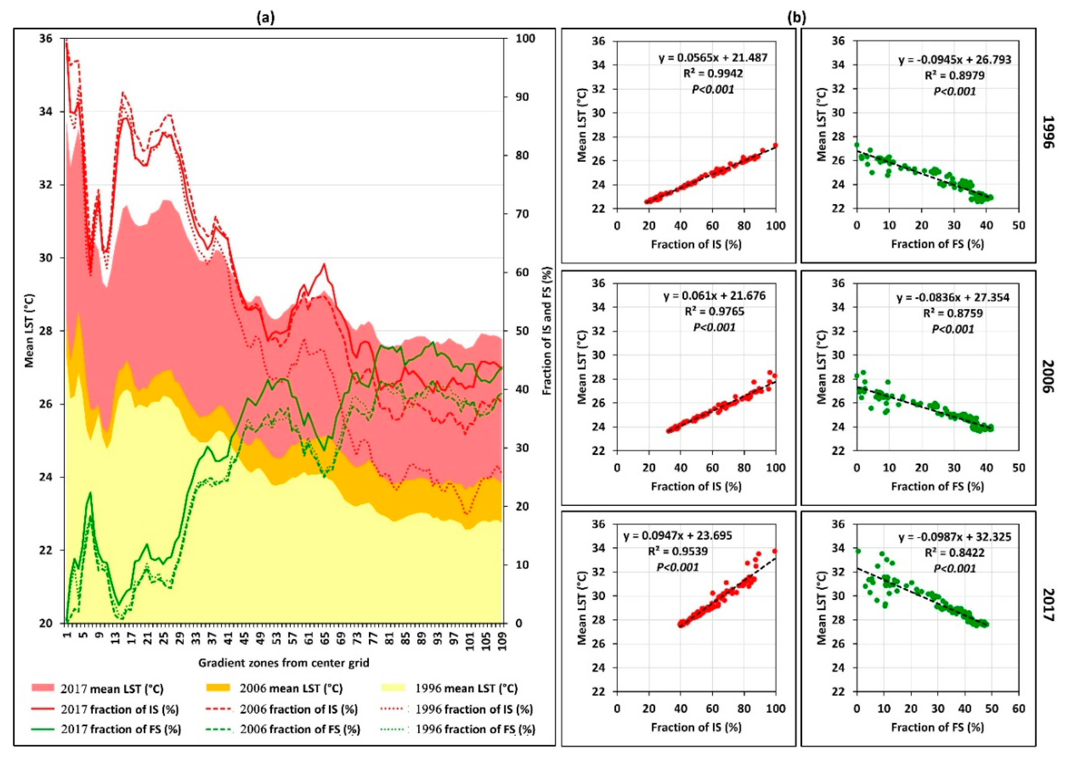
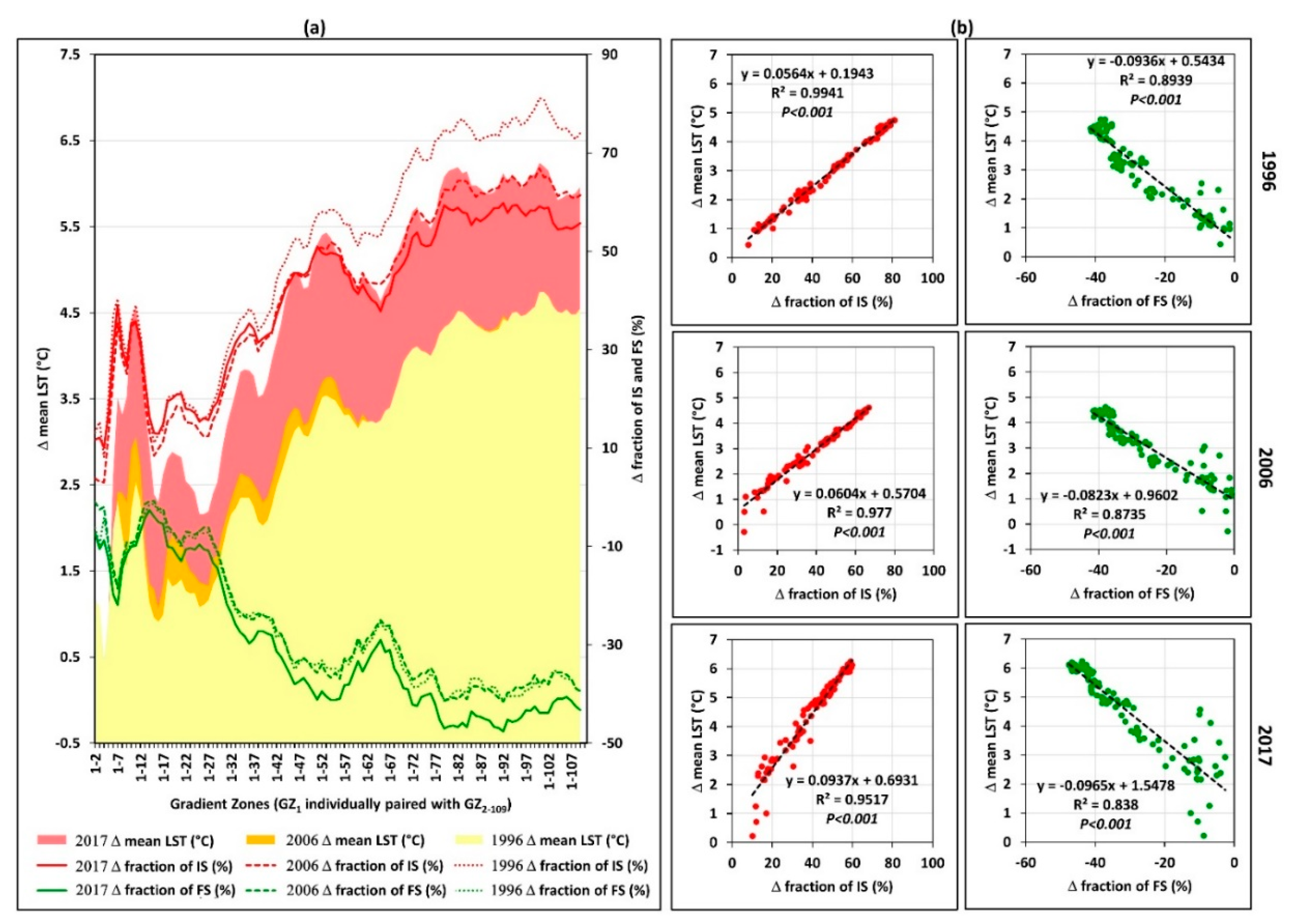
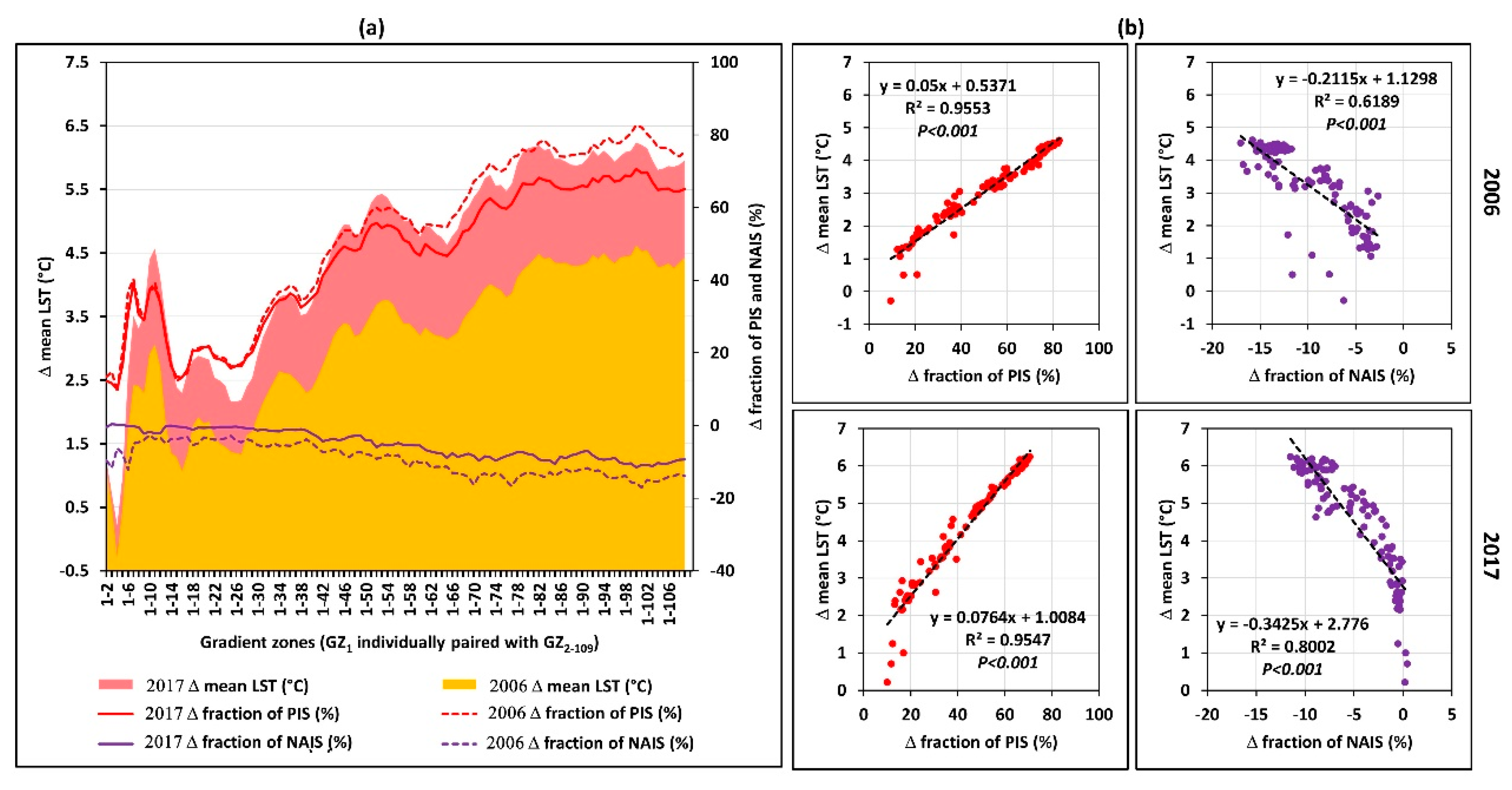
3.2.2. SUHIIGZ along the Gradient Zones

Figure 3a displays the spatial pattern of mean LST, and the fraction of IS and FS through the GZs in the three time points of 1996, 2006, and 2017. The spatial pattern of mean LST declined when moving away from the central zone for all three time points. It could also be observed that the spatial pattern of mean LST was relatively higher in 2017 than in 1996 and 2006 along the GZs. The mean LST values of all GZs in 2006 was higher than in 1996, but the difference is very low. However, in 2017, the mean LST of all GZs considerably increased when compared with the other two time points. The fraction ratio of IS gradually declined when moving away from the central zone, while the fraction ratio of FS gradually inclined for the same direction for all three time points. The results reflected the stronger influence of IS on SUHI along the GZs. Figure 3b shows the results of linear-regression analysis between the mean LST and the fraction of FS and IS. We observed a significant positive relationship (p < 0.001) between the fraction ratios of IS and mean LST with a higher coefficient of determination, while a negative relationship (p < 0.001) between the fraction ratios of FS and mean LST in 1996, 2006, and 2017. The positive relationship between the fraction of IS and mean LST was stronger than the negative relationship between the fraction ratio of FS and mean LST along the GZs for all three time points.
Most of the previous studies used a fraction of IS with mean LST without considering IS subdivisions [3,16,18]. In this research, we divided IS into PIS and NAIS to identify their impact to formulate SUHI. Figure 4a displays the spatial distribution of the mean LST and fraction of PIS and NAIS through the GZs in 2006 and 2017. The fraction of PIS shows an increasing pattern, while NAIS shows a decreasing trend. The fractional difference between PIS and NAIS is higher in the first half of the GZs from the central zone. Figure 4b shows the result of the linear regression between mean LST with PIS and NAIS. Mean LST had a strong significant positive relationship with a fraction of PIS. However, mean LST had a strong negative relationship with a fraction of NAIS in both time points. The results reflected the stronger influence of PIS on SUHI along the GZs.
Figure 5 shows the magnitude of ∆ mean LST, the ∆ fraction of IS and FS through the GZs in 1996, 2006, and 2017. The highest fraction of IS was recorded in GZ1 as 99.7%, 99.2%, and 99.2%, in 1996, 2006, and 2017, respectively, and the lowest fraction of IS recorded GZ92 (19.3 km away from the city center). The highest fraction of FS was recorded in the GZ92, where the lowest IS fraction was recorded. The lowest FS fraction was recorded in the GZ1. Figure 5b shows the results of linear-regression analysis based on all GZs in the three time points of 1996, 2006, and 2017, which showed a significant (p < 0.001) positive relationship between ∆ mean LST with ∆ fraction of IS. The ∆ mean LST had a strong negative relationship with a fraction of FS from 1996 to 2017. Similar results were obtained by previous studies as well [16,18].
Figure 6. shows the spatial distribution of the ∆ mean LST with the ∆ fraction of PIS, and the ∆ fraction of NAIS along the GZs in 2006 and 2017. IS magnitude is a piece of vital information to understand SUHI formation. The subdivisions of the IS fraction along the GZs provide an essential indicator to understand the SUHI of the study area. The ∆ fraction of PIS showed an increasing trend, especially after GZ42 (8.8 km from the city center). The decreasing trend of NAIS along the GZs was from 2006 to 2017. Figure 6b shows the results of the linear-regression analysis based on GZs in the two time points of 2006 and 2017. ∆ mean LST had a strong significant relationship with the ∆ fraction of PIS, while ∆ mean LST had a significantly strong negative relationship between the ∆ fraction of NAIS in both time points.

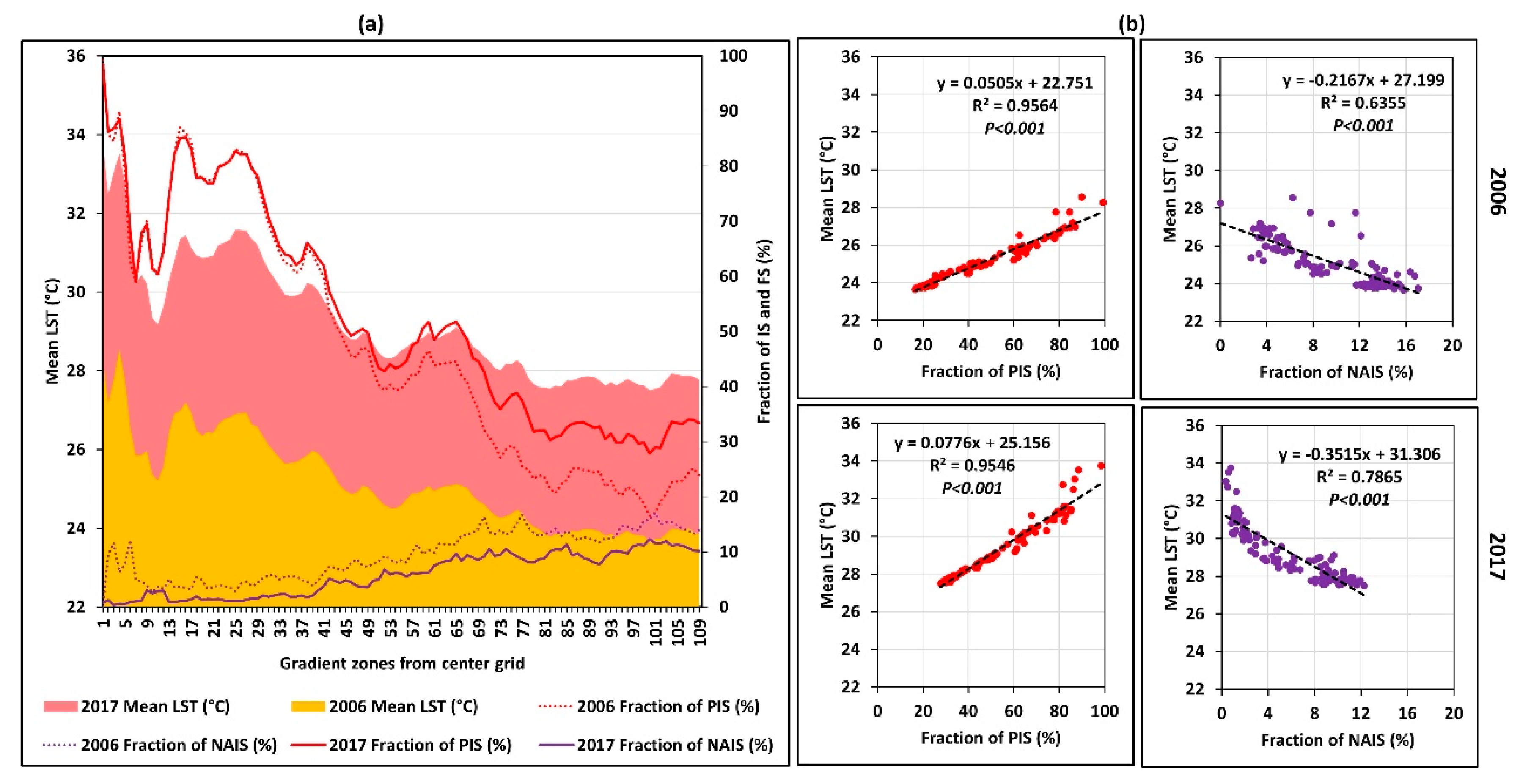
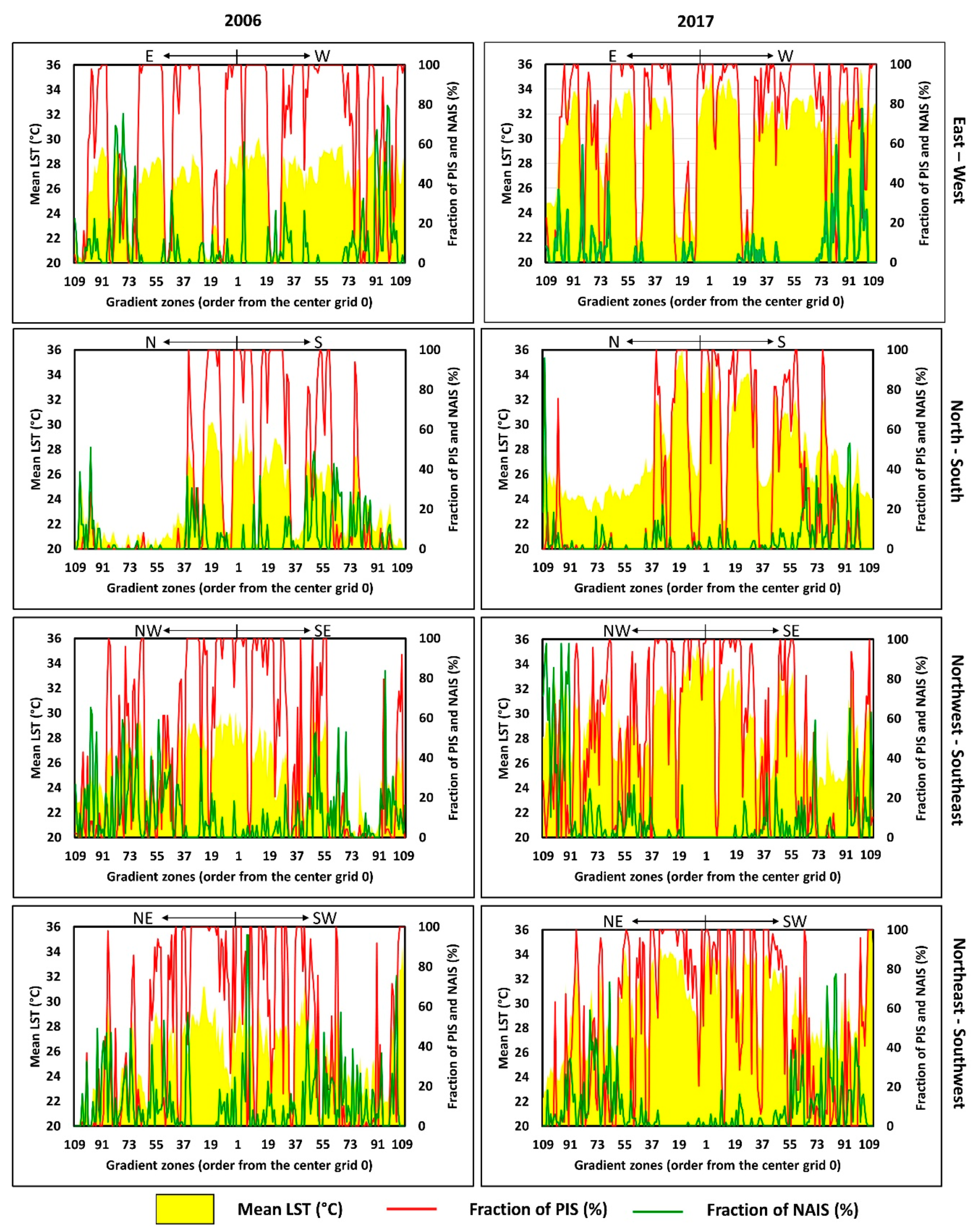
3.3. Multidirectional Analysis

Figure 7 shows multidirectional and multitemporal SUHI profiles based on mean LST, and the fractions of PIS and NAIS. According to the results, it is clearly shown that the directional distribution of SUHI magnitude was higher in the east–west direction in both 2006 and 2017. The typical SUHI profile can be seen in the northwest–southeast and northeast–southwest directions. In addition to that, the spatial distribution of the NAIS and PIS fractions shows that NAIS increased along the GZs outside the city center zone. The result shows that the spatial pattern of the mean LST of each direction had an increasing trend in 2017 when compared with 2006.

4. Discussion

4.1. Urbanization and Its Impact

Seoul is the capital city, and the business and the central financial hub of the Republic of Korea. The city is referred to as one of the emerging world cities in the Asia-Pacific region [55]. With the city’s geographical location in the Asia-Pacific region, Seoul has robust socioeconomic growth, with a gross domestic product (GDP) of USD 408 billion in 2016 [56]. LULC results in this study show that the city has experienced rapid urbanization during the last two decades (Figure 2a–c, and Table 3 and Table 4) with socioeconomic growth, especially in the east, west, northwest, southwest, and northeast of the study area. The IS of the study area reached 50.5% of the extent of total land in 2017. The growth rate of IS was 1,355.9 ha/year during the 1996–2017 period. Urban expansion during the 1996–2006 period showed a higher rate than the 2006–2017 period. This was mainly because of the city-development barriers due to geographical factors like rivers and mountains in the study area [55]. OL consisted of cropland, grassland, and bare land, which were replaced by IS during the past two decades. The total land extent of OL was 26.7% in 1996 from the total land extent, and it declined by up to 8.3% in 2017. Interestingly, the FS of the study area increased during the period of 1996–2017 with a rate of 541.5 ha/year, while it decreased during the period of 1996–2006 with a rate of 58.3 ha/year. The increase of FS was mainly because of the preservation of the natural environment with apartment parks and urban forests in the study area after 2006 [55].
Both the total and urban population of the Republic of Korea shows an increasing trend during the period of 1980–2030 [57]. In 2015, the total and urban population of the Republic of Korea were 51 and 41 million people, respectively. According to predictions, the total and urban population of the country will be 53 and 43 million, respectively, in 2030. According to statistics, over one-fifth of the nation’s total population lives in Seoul [55]. The total population of Seoul was saturated during the last decade [58], mainly because of higher apartment prices [55]. As a result, the concept of satellite towns was promoted in surrounding areas and people tend to stay in surrounding areas of the city. This lead to the rapid urbanization of the surrounding areas with the increase of population [55]. This study focused on Seoul and the surrounding areas, so the increasing trend of urban population can be used as a proxy indicator for the study area [3]. The population trend validated the urbanization process in the study area. The increasing trend of the number of vehicles in Seoul [59] also revalidated rapid urbanization in surrounding areas because residents of the surrounding areas use vehicles for transport to and from the city. According to statistics, there were around two million cars in 2000 and around three million cars in 2015 registered in Seoul [59].
With the increase of population, additional space is required for settlements, industrial zones, and infrastructure to cater to the urban community, and this leads to the expansion of urban areas (IS) by acquiring space from other LULC. This process was validated with the results of LULC changes during the period of study. IS reflects high amount of solar radiation when compared with other LULC, and this leads to generating heat back to the atmosphere, which tends to increase of LST in urban areas [18]. The results of the study validate that IS had a higher mean LST (Table 5a,b) than FS. According to Figure 2d–f, the higher distribution pattern of LST mirrored the distribution pattern of IS. The increasing trend of LST further improved with rapid urbanization in the study area during the period of study. This is a necessary consequence in the context of the UHI phenomenon.
Increasing urban population and increasing IS provide important information to rethink the present urban plan of the study area. A number of negative biophysical and socioeconomic consequences were identified as the result of the urban expansion and overpopulation of the study area [5,12]. Urban planners and policymakers need to consider controlling the SUHI in the study area.

4.2. Intensifying SUHI Effect

According to the results of the study, the mean LST of the study area relatively increased by 4.9 °C during the 1996–2017 study period. One of the exciting findings from the results is that the mean LST of NAIS was relatively lower than the mean LST of PIS and IS in 2006 and 2017 (Table 5a), which indicated that the NAIS was constructed on preserving the natural environment with apartment parks and urban forests [60]. During the study period, the average fraction of FS exhibited an increasing trend of 26.7%, 26.3%, and 31.3%, respectively, in 1996, 2006, and 2017. Previous studies show a decreasing trend of FS along the GZs due to the rapid urbanization in Asian cities [16,18]. This increasing FS trend was recorded due to the forest-conserving policy of the government of Seoul after 2006 [61,62]. Thus, NAIS developed with the considerable formation of the FS. According to the results, the relative difference of mean LST between PIS and NAIS was recorded at 1.5 °C in 2006 and 2.5 °C in 2017 (Table 5b, Figure 4b). NAIS shows the negative relationship with mean LST in the time points of 2006 and 2017. A similar relationship was recorded with a fraction of FS.
The combing effect of IS on LST remains as it is because, for a given time point, the total IS was constructed with the PIS from the previous time point plus the NAIS for the given time point. Moreover, the PIS for the next time point depended on the total IS of the previous time point (Equation (6)). The results of LST temporal variation among different LULC indicated rapid IS expansion, such as buildings, roads, parking lots, pavements, and other urban constructions by replacing green surfaces, which lead to intensifying the SUHI effect on the population of the study area.
I S 2017 = P I S 2006 + N A I S 2006 2017
where, IS2017 is IS in 2017; PIS2006–2017 is PIS during 2006–2017; and NAIS2006–2017 is NAIS during 2006–2017.
According to variations of the LST values, it was observed that there was an intensifying SUHI effect in the study area, but it did not describe the magnitude and trend of the effect. Therefore, the effect was studied along the GZs. It was observed that the mean LST declined along the GZs for all three time points (Figure 3 and Figure 4). It was also confirmed that the highest mean LST values were reported in GZ1 (near city center) as 27.3, 28.6, and 33.7 °C in 1996, 2006, and 2017, respectively. The results show that the mean temperature of GZ1 relatively increased by 6.4 °C in the past 21 years. An increasing pattern could be seen in a fraction of IS (49.2% in 1996, 57.1% in 2006, and 58.2% in 2017) and of PIS (47.7%, in 2006 and 52.6% in 2017). However, the fraction of the NAIS showed a decreasing pattern from 2006 to 2017. The average fraction of GZs decreased from 9.4% in 2006 to 5.9% in 2017. Urbanization was saturated in Seoul after 2006. There are very few spaces available for future urban development. Thus, more development happened vertically than horizontally, especially in the city center and surrounding areas. Vertical development can be used as a proxy indicator to understand urban-development intensity [63,64,65]. Results show that PIS had a strong significant relationship with the mean LST in 2006 and 2017 (Figure 4 and Figure 6). Thus, urban planners must pay considerable attention to introduce appropriate mitigation procedures, especially in PIS areas.
According to the results of the study, SUHII increased in the study area in 1996, 2006, and 2017 (Figure 5a and Figure 6a) with a high positive correlation (p < 0.001, high R2) with a fraction of IS for all three-time points. Further, there was a high negative correlation (p < 0.001, high R2) with a fractional difference of FS on SUHII in all three-time points (Figure 5b) that revalidated the importance of FS to minimize the SUHI effect. According to Figure 6b, there was a high positive correlation (p < 0.001, high R2) with a fractional difference of PIS on SUHII, which reconfirmed the stronger influence of PIS on SUHI than NAIS. The negative correlation (p < 0.001, high R2) with a fractional difference of NAIS on SUHII reconfirmed environmentally friendly urban constructions of the study area.
By using LST profiles generated through multidirectional analysis, the effect of PIS and NAIS on SUHI can be further visualized by mapping the cross-sectional features. According to Figure 7, it can be observed that the urbanization process taking place in the east–west direction was almost similar in 1996 and 2017, which indicated the limitation of urban development in that direction, which could also be confirmed with the LULC maps during the period (Figure 2a). The SUHI profile of the east–west direction shows that the increasing and decreasing pattern of the mean LST was followed by the fraction of PIS. The north–south direction showed the lowest mean LST profile due to the spatial distribution of the FS. The urban development of the other directions was limited except for the core of the city in 1996. However, in 2017, it could be observed that urban development took place in other directions of the study area. The positive correlation with the fraction of PIS on SUHI and negative correlation with the fraction of NAIS on SUHI were confirmed by observing the LST profiles of 2006 and 2017. The SUHI profile can be applied as a proxy indicator to understand the spatial distribution of the mean LST and fraction of PIS, and NAIS in 2006 and 2017.

4.3. Implications for Urban Sustainability

With the results in this study, we can argue that the observed increasing pattern of the SUHI effect in the research area was affected by LULC changes due to rapid urbanization, which caused in the rapid expansion of IS, and considerable loss of grassland and cropland over the past two decades. The SUHI effect in the study area can be considered as a local climate change [8,16]. The results of the study show that the spatial pattern of LST was comparatively lower in green surfaces, specifically in FS, than other LULC categories. Therefore, to mitigate the effect of SUHI, it is essential to improve the green-land fraction of the study, which provides more shade. Green surfaces can also absorb and reflect solar radiation, while evapotranspiration and shadowing make a more refreshing environment while minimizing the SUHI effect [37]. This can be verified with results of lower LST values reported in forest surfaces. On the other hand, the SUHI effect directly influences the increase of energy usage to reduce the temperature in living environments using air conditioners or other similar equipment [12]. Heat-related health issues may also arise in the city [13]. The decreasing trend of the green fraction in the city might influence food security, as well as imbalance ecosystem services in the city. To overcome these issues, appropriate measures need to be taken.
From the viewpoint of urban sustainability of the study area, government policies related to urban development need to further be improved to overcome issues that arise due to the SUHI effect. Past research has shown that urban parks and urban forests can mitigate LST in Seoul [36]. Further, improvements of green belts along roads can be considered, as well as the composition of as many green walls and roofs in future urban constructions as possible. Past research has also shown that green belts, walls, and roofs can mitigate the SUHI effect [13]. Additionally, they can improve LULC policies that relate to green-belt development [66]. According to our results, the increase of forest cover in 2017 indicated that the current LULC policies related to the green belt are active. Urban green network concepts such as urban forests, school forests, street trees, forest parks, and landscape forests were also included in Korean Urban Forest Policies [61,62]. Further, urban planners can promote the concept of satellite towns to mitigate urban construction related to housing facilities [55]. City planners should also further promote vertical urban developments as a space-conserving technique [67]. All these activities result from reducing LST and producing a cool-island effect that improves the natural air-circulation process to make a comfortable living atmosphere for the urban community. All these approaches allow sustainable urban development, which is in line with the goals of the 2030 agenda for sustainable development [56].
Finally, the authors would like to emphasize some of the light limitations of the study. By increasing the number of Landsat images in the summer season for a given year, it is possible to retrieve spatial and temporal information more preciously than by using a single image. But it is not possible to select multiple Landsat images in the summer season for a given year due to atmospheric distortions in the images mainly because of cloud cover. The previous studies also emphasized the same limitation in different Asian cities [16,18,51,68]. The timeframes 1996, 2006, and 2017 were selected based on the availability of the images as per the requirements stated in Section 2.2 by with the above-mentioned difficulty. Also, we understand that there are some other factors also affecting for LST other than LULC such as wind speed, surface moisture, humidity, and intensity of solar radiation. Because, the factors were not stable or stationary in the selected three time points. Therefore, the results were discussed with the focus on the spatial pattern of LST and its influence on the SUHI rather than the absolute values of LST or in other words a temporal pattern. Topographical factors such as surface height also influence for the difference of LST, but we did not consider in this study. By all means, the results were interpreted in the above-mentioned light limitations.

5. Conclusions

This study examined the effect of SUHI with its magnitude and trend in the city of Seoul and its surroundings as a geospatial study by using temporal Landsat data. For this purpose, we analyzed the relative variation of LST with LULC rather than absolute values along the gradient zones and different directions of the study area. It was observed that IS has expanded, and the SUHI effect was more penetrating in the study area, with a considerable loss of green surfaces along with the rapid urbanization of the study area. IS showed an increasing pattern, 37.2% to 50.5%, from the total land extent of the study area during the 21 years with 1355.5 ha/per year. This resulted from the increased temperature of the GZ1 by 6.4 °C. The mean LST difference between GZ1 and GZ109 showed an increasing pattern, from 4.6 °C in 1996 to 6.0 °C in 2017. We observed that the fraction of NAIS had a strong negative relationship with mean LST, and it has resulted in a declining SUHI in the study area. Crossover comparison results showed that FS recorded the relatively lowest temperature than the other LULC categories, and the second-lowest mean LST recorded in NAIS in 2006 and 2017.
Results proved that the local climate of Seoul and its surroundings were affected by the SUHI effect. Therefore, urban planners of the city of Seoul should seriously consider the issue and plan to mitigate the effect by improving the green surfaces of the city. Authors recommend to improve the urban greening concept that controls the effect of the SUHI. Considering all these, the authors conclude that the overall results of the study can be applied as a proxy indicator for the sustainability of Seoul and its surroundings.

Author Contributions

The corresponding author, P.P., has proposed the topic and spearheaded the data processing and analysis, as well as the writing of the manuscript. M.R., D.D., T.M., and Y.M. helped in the design, research implementation and analysis, and writing of the manuscript.

Funding

This study was supported by the Japan Society for the Promotion of Science (JSPS) through Grant-in-Aid for Scientific Research (B) 18H00763 (2018-20).

Acknowledgments

The authors express their gratitude to the anonymous reviewers and the editor for their valuable comments and suggestions to improve the manuscript.

Conflicts of Interest

The authors declare no conflict of interest.

Appendix A

Table A1. Error matrix for the 1996 LULC classification.
Classified DataReference DataTotalUser Accuracy (%)
FSISWBOL
Forest surface (FS)13430914691.78
Impervious surface (IS)020011021194.79
Water bodies (WB)101611888.89
Other lands (OL)26111612592.80
Total13720918136500
Producer accuracy (%)97.8195.6988.8985.29
Overall Accuracy = 93.20%.
Table A2. Error matrix for the 2007 LULC classification.
Classified DataReference DataTotalUser Accuracy (%)
FSISWBOL
Forest surface (FS)13811314396.50
Impervious surface (IS)62452726094.23
Water bodies (WB)001411593.33
Other lands (OL)450738289.02
Total1482511784500
Producer accuracy (%)93.2497.6182.3586.90
Overall Accuracy = 94.00%.
Table A3. Error matrix for the 2017 LULC classification.
Classified DataReference DataTotalUser Accuracy (%)
FSISWBOL
Forest surface (FS)16161217094.71
Impervious surface (IS)82592427394.87
Water bodies (WB)011601794.12
Other lands (OL)120374092.50
Total1702681943500
Producer accuracy (%)94.7196.6484.2186.05
Overall Accuracy = 94.60%.

References

  1. United Nations. World Urbanization Prospects: The 2018 Revision, Key Facts; United Nations: New York, NY, USA, 2015. [Google Scholar]
  2. Guo, L.; Liu, R.; Men, C.; Wang, Q.; Miao, Y.; Zhang, Y. Quantifying and simulating landscape composition and pattern impacts on land surface temperature: A decadal study of the rapidly urbanizing city of Beijing, China. Sci. Total. Environ. 2019, 654, 430–440. [Google Scholar] [CrossRef] [PubMed]
  3. Dissanayake, D.; Morimoto, T.; Murayama, Y.; Ranagalage, M. Impact of landscape structure on the variation of land surface temperature in Sub-Saharan region: A case study of Addis Ababa using Landsat Data (1986–2016). Sustainability 2019, 11, 2257. [Google Scholar] [CrossRef]
  4. Arsiso, B.K.; Tsidu, G.M.; Stoffberg, G.H.; Tadesse, T. Influence of urbanization-driven land use/cover change on climate: The case of Addis Ababa, Ethiopia. Phys. Chem. Earth Parts A/B/C 2018, 105, 212–223. [Google Scholar] [CrossRef]
  5. Environmental Protection Agency (EPA). Reducing Urban Heat Islands: Compendium of Strategies. Heat Island Reduction Activities; EPA: Washington, DC, USA, 2008.
  6. Huang, C.-H.; Lin, P.-Y. The influence of evapotranspiration by urban greenery on thermal environment in urban microclimate. Int. Rev. Spat. Plan. Sustain. Dev. 2013, 1, 1–12. [Google Scholar] [CrossRef]
  7. Voogt, J.; Oke, T. Thermal remote sensing of urban climates. Remote Sens. Environ. 2003, 86, 370–384. [Google Scholar] [CrossRef]
  8. Environmental Protection Agency (EPA). Reducing Urban Heat Islands: Compendium of Strategies Urban Heat Island Basics; EPA: Washington, DC, USA, 2008.
  9. Mirzaei, P.A.; Haghighat, F. Approaches to study urban heat island—abilities and limitations. Build. Environ. 2010, 45, 2192–2201. [Google Scholar] [CrossRef]
  10. Estoque, R.C.; Murayama, Y. Measuring sustainability based upon various perspectives: A case study of a hill station in Southeast Asia. Ambio 2014, 43, 943–956. [Google Scholar] [CrossRef] [PubMed]
  11. Estoque, R.C.; Murayama, Y. Quantifying landscape pattern and ecosystem service value changes in four rapidly urbanizing hill stations of Southeast Asia. Landsc. Ecol. 2016, 31, 1481–1507. [Google Scholar] [CrossRef]
  12. Memon, R.A.; Leung, D.Y.C.; Chunho, L. A review on the generation, determination and mitigation of urban heat island. J. Environ. Sci. 2008, 20, 120–128. [Google Scholar]
  13. Heaviside, C.; MacIntyre, H.; Vardoulakis, S. The urban heat island: implications for health in a changing environment. Curr. Environ. Health Rep. 2017, 4, 296–305. [Google Scholar] [CrossRef]
  14. Ranagalage, M.; Estoque, R.C.; Murayama, Y. An urban heat island study of the Colombo Metropolitan Area, Sri Lanka, based on Landsat Data (1997–2017). ISPRS Int. J. Geo-Inf. 2017, 6, 189. [Google Scholar] [CrossRef]
  15. Ranagalage, M.; Estoque, R.C.; Zhang, X.; Murayama, Y. Spatial changes of urban heat island formation in the Colombo District, Sri Lanka: implications for sustainability planning. Sustainability 2018, 10, 1367. [Google Scholar] [CrossRef]
  16. Estoque, R.C.; Murayama, Y. Monitoring surface urban heat island formation in a tropical mountain city using Landsat data (1987–2015). ISPRS J. Photogramm. Remote Sens. 2017, 133, 18–29. [Google Scholar] [CrossRef]
  17. Dissanayake, D.; Morimoto, T.; Ranagalage, M.; Murayama, Y. Land-use/land-cover changes and their impact on surface urban heat islands: Case study of Kandy city, Sri Lanka. Climate 2019, 7, 99. [Google Scholar] [CrossRef]
  18. Ranagalage, M.; Dissanayake, D.; Murayama, Y.; Zhang, X.; Estoque, R.C.; Perera, E.; Morimoto, T. Quantifying surface urban heat island formation in the world heritage tropical mountain city of Sri Lanka. ISPRS Int. J. Geo-Inf. 2018, 7, 341. [Google Scholar] [CrossRef]
  19. Simwanda, M.; Ranagalage, M.; Estoque, R.C.; Murayama, Y. Spatial analysis of surface urban heat islands in four rapidly growing African Cities. Remote Sens. 2019, 11, 1645. [Google Scholar] [CrossRef]
  20. Rousta, I.; Sarif, M.O.; Gupta, R.D.; Olafsson, H.; Ranagalage, M.; Murayama, Y.; Zhang, H.; Mushore, T.D. Spatiotemporal analysis of land use/land cover and its effects on surface urban heat island using Landsat data: A case study of metropolitan city Tehran (1988–2018). Sustainability 2018, 10, 4433. [Google Scholar] [CrossRef]
  21. Oke, T.R. Initial Guidance to Obtain Representative Meteorological Observations at Urban Sites; World Meteorological Organization (WMO): Geneva, Switzerland, 2006. [Google Scholar]
  22. Stewart, I.; Oke, T. Classifying urban climate field sites by “local climate zones”: The case of Nagano, Japan. In Proceedings of the Seventh International Conference on Urban Climate, Yokohama, Japan, 29 June–3 July 2009; pp. 1–5. [Google Scholar]
  23. Gunaalan, K.; Ranagalage, M.; Gunarathna, M.H.J.P.; Kumari, M.K.N.; Vithanage, M.; Srivaratharasan, T.; Saravanan, S.; Warnasuriya, T. Application of geospatial techniques for groundwater quality and availability assessment: A case study in Jaffna Peninsula, Sri Lanka. ISPRS Int. J. Geo-Inf. 2018, 7, 20. [Google Scholar] [CrossRef]
  24. Weng, Q.; Lu, D.; Schubring, J. Estimation of land surface temperature–vegetation abundance relationship for urban heat island studies. Remote Sens. Environ. 2004, 89, 467–483. [Google Scholar] [CrossRef]
  25. Demissie, F.; Yeshitila, K.; Kindu, M.; Schneider, T. Land use/land cover changes and their causes in Libokemkem District of South Gonder, Ethiopia. Remote Sens. Appl. Soc. Environ. 2017, 8, 224–230. [Google Scholar] [CrossRef]
  26. Kindu, M.; Schneider, T.; Teketay, D.; Knoke, T. Land Use/land cover change analysis using object-based classification approach in Munessa-Shashemene landscape of the Ethiopian Highlands. Remote Sens. 2013, 5, 2411–2435. [Google Scholar] [CrossRef]
  27. Dissanayake, D.; Morimoto, T.; Ranagalage, M. Accessing the soil erosion rate based on RUSLE model for sustainable land use management: A case study of the Kotmale watershed, Sri Lanka. Model. Earth Syst. Environ. 2018, 5, 291–306. [Google Scholar] [CrossRef]
  28. Ranagalage, M.; Wang, R.; Gunarathna, M.H.J.P.; Dissanayake, D.M.S.L.B.; Murayama, Y.; Simwanda, M. Spatial forecasting of the landscape in rapidly urbanizing hill stations of south asia: A case study of Nuwara Eliya, Sri Lanka (1996–2037). Remote Sens. 2019, 11, 1743. [Google Scholar] [CrossRef]
  29. Mellor, A.; Haywood, A.; Stone, C.; Jones, S. The performance of random forests in an operational setting for large area sclerophyll forest classification. Remote Sens. 2013, 5, 2838–2856. [Google Scholar] [CrossRef]
  30. Goslee, S.C. Analyzing remote sensing data in R: The Landsat package. J. Stat. Softw. 2015, 43. [Google Scholar] [CrossRef]
  31. Nguyen, G.; Dlugolinsky, S.; Bobák, M.; Tran, V.; García, Á.L.; Heredia, I.; Malík, P.; Hluchý, L. Machine learning and deep learning frameworks and libraries for large-scale data mining: A survey. Artif. Intell. Rev. 2019, 52, 77–124. [Google Scholar] [CrossRef]
  32. Kamusoko, C.; Gamba, J.; Murakami, H. Mapping woodland cover in the Miombo ecosystem: A comparison of machine learning classifiers. Land 2014, 3, 524–540. [Google Scholar] [CrossRef]
  33. Liu, Y.; Peng, J.; Wang, Y. Efficiency of landscape metrics characterizing urban land surface temperature. Landsc. Urban Plan. 2018, 180, 36–53. [Google Scholar] [CrossRef]
  34. Tran, H.; Uchihama, D.; Ochi, S.; Yasuoka, Y. Assessment with satellite data of the urban heat island effects in Asian mega cities. Int. J. Appl. Earth Obs. Geoinf. 2006, 8, 34–48. [Google Scholar] [CrossRef]
  35. Estoque, R.C.; Murayama, Y.; Myint, S.W. Effects of landscape composition and pattern on land surface temperature: An urban heat island study in the megacities of Southeast Asia. Sci. Total Environ. 2017, 577, 349–359. [Google Scholar] [CrossRef] [PubMed]
  36. Kil, S.-H.; Yun, Y.-J. Understanding the LST (Land Surface Temperature) effects of urban-forests in Seoul, Korea. J. For. Environ. Sci. 2018, 34, 246–248. [Google Scholar]
  37. Choi, Y.-Y.; Suh, M.-S.; Park, K.-H. Assessment of surface urban heat islands over three megacities in East Asia using land surface temperature data retrieved from COMS. Remote Sens. 2014, 6, 5852–5867. [Google Scholar] [CrossRef]
  38. Spatial Information Science Laboratory (SIS). Megacities Project. Available online: http://giswin.geo.tsukuba.ac.jp/mega-cities/asia_index.html (accessed on 9 July 2019).
  39. United Nations. World Urbanization Prospects. Available online: https://population.un.org/wup/Download/ (accessed on 9 July 2019).
  40. Ma, S.; An, S.; Park, D. Urban-rural migration and migrants’ successful settlement in Korea. Dev. Soc. 2018, 47, 285–312. [Google Scholar]
  41. United Nations. Social and Solidarity Economy for the Sustainable Development Goals: Spotlight on the Social Economy in Seoul; UNRISD: Geneva, Switzerland, 2018. [Google Scholar]
  42. Park, S.; Lim, J.; Lim, H.S. Past climate changes over South Korea during MIS3 and MIS1 and their links to regional and global climate changes. Quat. Int. 2019, 519, 74–81. [Google Scholar] [CrossRef]
  43. Lee, D.; Oh, K. Classifying urban climate zones (UCZs) based on statistical analyses. Urban Clim. 2018, 24, 503–516. [Google Scholar] [CrossRef]
  44. Geographic Guide. World in Images—Tourist Destinations. Available online: http://www.geographicguide.net/ (accessed on 18 April 2019).
  45. DIVA-GIS. DIVA-GIS|Free, Simple, and Effective. Available online: http://www.diva-gis.org/ (accessed on 18 April 2019).
  46. USGS. EarthExplorer—Home. Available online: https://earthexplorer.usgs.gov/ (accessed on 18 April 2019).
  47. USGS. Landsat Science Products. Available online: https://www.usgs.gov/land-resources/nli/landsat/landsat-science-products (accessed on 18 April 2019).
  48. Estoque, R.C.; Murayama, Y. Classification and change detection of built-up lands from Landsat-7 ETM+ and Landsat-8 OLI/TIRS imageries: A comparative assessment of various spectral indices. Ecol. Indic. 2015, 56, 205–217. [Google Scholar] [CrossRef]
  49. Stehman, S.V. Sampling designs for accuracy assessment of land cover. Int. J. Remote Sens. 2009, 30, 5243–5272. [Google Scholar] [CrossRef]
  50. Sobrino, J.A.; Jiménez-Muñoz, J.C.; Paolini, L. Land surface temperature retrieval from LANDSAT TM 5. Remote Sens. Environ. 2004, 90, 434–440. [Google Scholar] [CrossRef]
  51. Ranagalage, M.; Estoque, R.C.; Handayani, H.H.; Zhang, X.; Morimoto, T.; Tadono, T.; Murayama, Y. Relation between urban volume and land surface temperature: A comparative study of planned and traditional cities in Japan. Sustainability 2018, 10, 2366. [Google Scholar] [CrossRef]
  52. Dissanayake, D.; Morimoto, T.; Murayama, Y.; Ranagalage, M.; Handayani, H.H. Impact of urban surface characteristics and socio-economic variables on the spatial variation of land surface temperature in Lagos city, Nigeria. Sustainability 2019, 11, 25. [Google Scholar] [CrossRef]
  53. Myint, S.W.; Brazel, A.; Okin, G.; Buyantuyev, A. Combined effects of impervious surface and vegetation cover on air temperature variations in a rapidly expanding desert city. GISci. Remote Sens. 2010, 47, 301–320. [Google Scholar] [CrossRef]
  54. Ye, S.; Pontius, R.G.; Rakshit, R. A review of accuracy assessment for object-based image analysis: From per-pixel to per-polygon approaches. ISPRS J. Photogramm. Remote Sens. 2018, 141, 137–147. [Google Scholar] [CrossRef]
  55. Kim, H.M.; Han, S.S. Seoul. Cities 2012, 29, 142–154. [Google Scholar] [CrossRef]
  56. United Nations. Transforming Our World: The 2030 Agenda for Sustainable Development; United Nations General Assembly: New York, NY, USA, 2015; Volume 16301, pp. 1–35. [Google Scholar]
  57. United Nations. World Population Prospects. Available online: https://population.un.org/wpp/ (accessed on 12 April 2019).
  58. Jeong, J.-C. The land surface temperature analysis of Seoul city using Satellite Image. J. Environ. Impact Assess. 2013, 22, 19–26. [Google Scholar] [CrossRef]
  59. Shin, J.; Park, H.; Seo, J.; Lee, J.; Park, H. Analysis of local and periodical transition in Cheong-Gye-Cheon to harmonize locality for urban green growth. KSCE J. Civ. Eng. 2015, 19, 2005–2016. [Google Scholar] [CrossRef]
  60. Huang, C.; Ye, X. Spatial modeling of urban vegetation and land surface temperature: A case study of Beijing. Sustainability 2015, 7, 9478–9504. [Google Scholar] [CrossRef]
  61. Korea Forest Service. Korea Urban Forest Policies; Korea Forest Service: Daejeon, Korea, 2006.
  62. Korea Forest Service. Forest Policy. Available online: http://english.forest.go.kr/newkfsweb/html/EngHtmlPage.do?pg=/esh/policy/UI_KFS_0102_010500.html&mn=ENG_02_01_05 (accessed on 29 July 2019).
  63. Estoque, R.C.; Murayama, Y.; Ranagalage, M.; Hou, H.; Subasinghe, S. Validating ALOS PRISM DSM-derived surface feature height: Implications for urban volume estimation. Tsukuba Geoenviron. Sci. 2017, 20, 378–383. [Google Scholar]
  64. Ranagalage, M.; Murayama, Y. Measurement of urban built-up volume using remote sensing data and geospatial techniques. Tsukuba Geoenviron. Sci. 2018, 14, 19–29. [Google Scholar]
  65. Handayani, H.H.; Murayama, Y.; Ranagalage, M.; Liu, F.; Dissanayake, D. Geospatial analysis of horizontal and vertical urban expansion using multi-spatial resolution data: A case study of Surabaya, Indonesia. Remote Sens. 2018, 10, 1599. [Google Scholar] [CrossRef]
  66. Han, H.; Huang, C.; Ahn, K.-H.; Shu, X.; Lin, L.; Qiu, D. The effects of greenbelt policies on land development: Evidence from the deregulation of the greenbelt in the Seoul Metropolitan Area. Sustainability 2017, 9, 1259. [Google Scholar] [CrossRef]
  67. Zhang, W.; Li, W.; Zhang, C.; Hanink, D.M.; Liu, Y.; Zhai, R. Analyzing horizontal and vertical urban expansions in three East Asian megacities with the SS-coMCRF model. Landsc. Urban Plan. 2018, 177, 114–127. [Google Scholar] [CrossRef]
  68. Zhang, X.; Estoque, R.C.; Murayama, Y. An urban heat island study in Nanchang City, China based on land surface temperature and social-ecological variables. Sustain. Cities Soc. 2017, 32, 557–568. [Google Scholar] [CrossRef]
Figure 1. Location map of the study area. (a) Map of Southeast Asia with the Republic of Korea [44]; (b) location of the Seoul metropolitan area (SMA) [45]; and (c) study area within the SMA (Landsat-8 OLI/TIRS in false-color composite (Bands 5, 4, 3; 26 August 2017) with the city center [46].
Climate 07 00110 g001
Figure 2. LULC and land-surface temperature (LST) of the study area. LULC in (a) 1996, (b) 2006, and (c) 2017; LST in (d) 1996; (e) 2006; and (f) 2017.
Climate 07 00110 g002
Figure 3. (a) Spatial pattern of mean LST and the fraction of IS and FS along the gradient zones (GZs); and (b) scatter plots between mean LST and fraction of IS and FS in 1996, 2006, and 2017.
Climate 07 00110 g003
Figure 4. (a) Spatial distribution of mean LST and fraction of PIS and NAIS through the GZs; and (b) scatter plots among mean LST and fraction of PIS and NAIS in 2006, and 2017.
Climate 07 00110 g004
Figure 5. (a) Magnitude of SUHII trend and fractional difference of IS and FS along the GZs. (b) Scatter plots and statistical relationship between the difference of mean LST and fractional difference of IS and FS along GZs in 1996, 2006, and 2017.
Climate 07 00110 g005
Figure 6. (a) Magnitude of Surface Urban Heat Island Intensity (SUHII) trend and fractional difference of PIS and NAIS along the GZs; (b) scatter plots and statistical relationship between SUHII magnitude and fractional difference of PIS and NAIS in 2006 and 2017.
Climate 07 00110 g006
Figure 7. Multitemporal and multidirectional surface urban heat island (SUHI) profiles of the study area based on mean LST, a fraction of PIS and NAIS.
Climate 07 00110 g007
Table 1. Landsat Level 2 data collection.
SensorLandsat-5 TMLandsat-5 TMLandsat-8 OLI/TIRS
Scene IDLT51160341996245CLT00LT51160342006256IKR00LC81160342017238LGN00
Temporal Resolution01 September 199613 September 200626 August 2017
Path/Row116/34
Local Time (GMT+9) *10:27:5911:04:4811:11:08
* GMT is known as Greenwich Mean Time
Table 2. Accuracies and kappa coefficient of land use/land cover (LULC) classifications in the SMA. Note: forest surface (FS); impervious surface (IS); water bodies (WB); and other lands (OL).
AccuracyLULC Category199620062017
User accuracy (%)Forest surface (FS)91.7896.5094.71
Impervious surface (IS)94.7994.2394.87
Water bodies (WB)88.8993.3394.12
Other lands (OL)92.8089.0292.50
Producer accuracy (%)Forest surface (FS)97.8193.2494.71
Impervious surface (IS)95.6997.6196.64
Water bodies (WB)88.8982.3584.21
Other lands (OL)85.2986.9086.05
Overall accuracy (%)93.2094.0094.60
Kappa coefficient0.900.900.91
Table 3. LULC composition in 1996, 2006, and 2017.
LULC199620062017
Area (ha)%Area (ha)%Area (ha)%
FS70,734.133.170,150.732.982,105.938.5
IS79,379.437.2100,335.347.0107,853.5 50.5
WB6331.53.05216.02.45702.22.7
OL56,999.026.737,742.017.717,782.48.3
Total213,444.0100.0213,444.0100.0213,444.0100.0
Table 4. LULC changes in 1996–2006, 2006–2017, and 1996–2017.
1996–20062006–20171996–2017
LULCLULC Change (ha)Growth Rate (ha/year)LULC Change (ha)Growth Rate (ha/year)LULC Change (ha)Growth Rate (ha/year)
FS−583.4−58.311,955.21086.811,371.8541.5
IS20,955.92095.67518.2683.528,474.11355.9
WB−1115.5−111.6486.244.2−629.3−30.0
OL−19,257.0−1925.7−19,959.6−1814.5−39,216.6−1867.5
Table 5. (a) Mean LST of FS, IS, persistent IS (PIS), and newly added IS (NAIS); (b) magnitude and trend of surface urban heat island intensity (SUHII).
(a) Mean LST of FS, IS, PIS, and NAIS (°C)
LULC20062017
FS21.425.6
IS27.131.1
PIS27.531.5
NAIS26.029.0
(b) Magnitude and trend of SUHII (°C)
LULC (cross-cover comparison)20062017
IS–PIS−0.4−0.4
IS–NAIS1.22.1
PIS–NAIS1.52.5
IS–FS5.75.5
PIS–FS6.15.9
NAIS–FS4.53.4

