The Origin and Propagation of the Antarctic Centennial Oscillation


1
Division of Physical and Biological Sciences, University of California, Santa Cruz, CA 95064, USA
2
Environmental Studies Institute, Santa Cruz, CA 95062, USA
*
Author to whom correspondence should be addressed.
Climate 2019, 7(9), 112; https://0-doi-org.brum.beds.ac.uk/10.3390/cli7090112
Submission received: 9 May 2019
/
Revised: 18 August 2019
/
Accepted: 23 August 2019
/
Published: 17 September 2019
Abstract
:The Antarctic Centennial Oscillation (ACO) is a paleoclimate temperature cycle that originates in the Southern Hemisphere, is the presumptive evolutionary precursor of the contemporary Antarctic Oscillation (AAO), and teleconnects to the Northern Hemisphere to influence global temperature. In this study we investigate the internal climate dynamics of the ACO over the last 21 millennia using stable water isotopes frozen in ice cores from 11 Antarctic drill sites as temperature proxies. Spectral and time series analyses reveal that ACOs occurred at all 11 sites over all time periods evaluated, suggesting that the ACO encompasses all of Antarctica. From the Last Glacial Maximum through the Last Glacial Termination (LGT), ACO cycles propagated on a multicentennial time scale from the East Antarctic coastline clockwise around Antarctica in the streamline of the Antarctic Circumpolar Current (ACC). The velocity of teleconnection (VT) is correlated with the geophysical characteristics of drill sites, including distance from the ocean and temperature. During the LGT, the VT to coastal sites doubled while the VT to inland sites decreased fourfold, correlated with increasing solar insolation at 65°N. These results implicate two interdependent mechanisms of teleconnection, oceanic and atmospheric, and suggest possible physical mechanisms for each. During the warmer Holocene, ACOs arrived synchronously at all drill sites examined, suggesting that the VT increased with temperature. Backward extrapolation of ACO propagation direction and velocity places its estimated geographic origin in the Southern Ocean east of Antarctica, in the region of the strongest sustained surface wind stress over any body of ocean water on Earth. ACO period is correlated with all major cycle parameters except cycle symmetry, consistent with a forced, undamped oscillation in which the driving energy affects all major cycle metrics. Cycle period and symmetry are not discernibly different for the ACO and AAO over the same time periods, suggesting that they are the same climate cycle. We postulate that the ACO/AAO is generated by relaxation oscillation of Westerly Wind velocity forced by the equator-to-pole temperature gradient and propagated regionally by identified air-sea-ice interactions.
Keywords:
Antarctic Circumpolar Current; Antarctic Circumpolar Vortex; Antarctic drill sites; Antarctic Oscillation; anthropogenic global warming; climate policy; Holocene; ice cores; Last Glacial Maximum; Last Glacial Termination; natural climate cycle; natural global warming; relaxation oscillation; Southern Annular Mode; stable isotope temperature proxies; teleconnection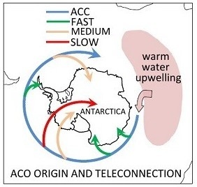
1. Introduction
Oscillation is a universal feature of climate across all spatial and temporal scales. The repetition period of natural climate cycles varies over ten orders of magnitude, from approximately 135–150 million years (My) for Phanerozoic temperature oscillations [1,2] to approximately 80–120 thousand years (Ky) for planetary “Great Ice Ages” or Marine Isotope Stages (MISs) [3,4], approximately 3–11 years (y) for the El Niño-Southern Oscillation (ENSO) [5,6,7], and approximately 40–50 days for the Madden-Julian Oscillation [8,9,10]. Forces external to the Earth, such as periodic variation in solar insolation at the surface induced by natural perturbations of Earth’s orbital cycles, drive at least some of these natural climate cycles [3], but in no case are the Earth’s internal responses to such external forcing fully understood. In the present study we investigate one such cycle, the Antarctic Centennial Oscillation (ACO) [11] over the past approximately 21,000 y from the Last Glacial Maximum (LGM) to the present. The primary purpose of our study is to elucidate the internal climate dynamics of the ACO, including its regional distribution, teleconnection, geographic source, and method of generation.
A secondary purpose of our study is to explore the relationship between the ACO and its postulated contemporary counterpart, the Antarctic Oscillation (AAO), known also as the Southern Annular Mode (SAM). Growing evidence suggests that the ACO and the AAO/SAM are the same natural climate cycle manifested at different times in paleoclimate history. To cite just one congruence, over the last millennium, the ACO as manifest in paleoclimate data oscillated at a mean period of 146 y [11] (Supplementary Material (SM), Table S1), placing it near the median order-of-magnitude ranking of periodicity for known climate cycles. Over the same time period, the AAO as manifest in contemporary climate data oscillated at a mean period of 143 y [12] (blue curve in their Figure 1a), comparable within likely error limits to the repetition frequency of the ACO. The similarity of their respective oscillation frequencies, as extended and expanded in this study, is consistent with the hypothesis that the ACO and AAO/SAM are the same natural climate cycle.
Previous investigators have observed that “despite the clear importance of the SAM (i.e., AAO) in the modern/future climate, very little is known regarding its behavior during pre-industrial times” [13] (p. 1). If the ACO and the AAO/SAM are the same natural climate cycle, discovery of the ACO in multiple paleoclimate records over hundreds of millennia before the onset of the Industrial Age ([11], this paper) promises to provide the missing historical record of the AAO. In this case, understanding the ACO is expected to illuminate the AAO, and conversely. Additionally, clarifying the climate dynamics of the ACO and AAO may provide insight into the internal mechanisms of a broader spectrum of climate oscillations, including for example the recurrent Great Ice Ages (MISs) that dominate contemporary climate on multimillennial time scales.
Additional impetus for this study stems from the finding by several investigators that large temperature excursions in the Southern Hemisphere (SH) are reflected quickly in the Northern Hemisphere (NH), raising the possibility that the ACO contributes to contemporary global warming. For example, the ENSO propagates on an annual time scale to the NH to induce temperature changes up to 2 °C [14]. Similarly, the ACO is the proximate source of Dansgaard-Oeschger (D-O) oscillations of 5–8 °C in Greenland ice cores, showing that the ACO strongly influences temperature in the NH [11]. The amplitude and rate of these natural global temperature excursions forced from the SH exceed the contemporary global warming signal of approximately 0.8 °C since 1880 [15] by up to 1–3 orders of magnitude. Therefore, natural temperature cycles in the SH may have contributed to the global warming signal in the NH over the past 140 y. In this case, elucidating the climate dynamics of the ACO/AAO may assist our understanding of contemporary global climate change and inform the development of correspondingly-adaptive climate policies.
Toward these ends, this study expands our previous investigation of the ACO from four Antarctic drill sites on the East Antarctic Plateau (EAP) to 11 drill sites distributed widely across the Antarctic continent. We apply the identical rationale and analytic approach published previously [11] to the larger sample of paleoclimate records. In the process we develop new empirical evidence that the ACO enveloped all of Antarctica and teleconnected on a multicentennial time scale clockwise around and across the Antarctic continent. We use this new empirical evidence to estimate the geographic site of generation of the ACO in the Southern Ocean (SO) east of Antarctica, and we explore the underlying climate mechanisms through correlation analysis of ACO cycle parameters. Finally, we show that key quantitative metrics of the paleoclimate ACO cycle and the contemporary AAO cycle over the same time periods are not discernibly different, adding to the growing evidence that the ACO and the AAO/SAM are past and present expressions, respectively, of the same natural climate cycle.
In the final section of this paper (Conclusions and Hypotheses) we attempt to integrate our empirical findings with existing knowledge of atmospheric and oceanic processes in a unified theory of ACO/AAO generation and regional teleconnection. We postulate that the ACO/AAO arises from relaxation oscillation (RO) of Westerly Winds (WWs) forced thermodynamically by the temperature gradient between the equator and the poles and buffered by the Antarctic cryosphere as modulated by variation in sea surface temperature (SST) within the Antarctic Circumpolar Current (ACC). This integrated hypothesis of ACO/AAO climate dynamics can account for the generation and teleconnection of the ACO/AAO, although significant puzzles remain. This integrated hypothesis can also help explain disparate and previously-puzzling Antarctic phenomena, including the pattern of sea ice distribution around Antarctica during the LGM and at present; the spatio-temporal course of sea-ice retreat during the LGT, the early Holocene, and seasonally; the temperature difference between West and East Antarctica; and the “climate memory” intrinsic to the Antarctic climate system [11].
2. Methods
2.1. Data Sources
The paleoclimate temperature-proxy records used in this study are labeled following the alphanumeric system developed previously for the ACO at Vostok [11] and tabulated by drill site in the Supplementary Material, Tables S1 and S2. Every result of the present study can be replicated using these open-access data in combination with data available from other sources cited. Information contained in the Supplementary Material enables independent confirmation of the data used here against the sources cited, facilitates replication of all results reported here, and supports further independent analysis of the ACO/AAO.
Open-access databases containing temperature proxies (deuterium, δ2H (‰) and oxygen, δ18O (‰)) from Antarctic ice cores were downloaded from the paleoclimate databases published by the World Paleoclimate Data Center (WPDC), United States National Oceanic and Atmospheric Administration (NOAA) [16]. Ice-core datasets analyzed here and their sources include Vostok [17,18], the European Project for Ice Coring in Antarctica (EPICA) Dome C (EDC) (updated EDC3 age model) [19,20,21], Law Dome (LD) [22,23], Taylor Dome (TD) [24,25], Talos Dome (TALDICE) [22,23], Siple Dome (SD) [22,23], Byrd Dome [22,23], James Ross Island (JRI) [26], EPICA Dronning Maud Land (EDML) [22,23], Dome Fuji (DF) [27,28], and EPICA Dome B (EDB) [29].
To measure latencies between ACOs at Vostok and their identified homologs at other drill sites, we used the most accurate paleoclimate chronologies available wherever applicable, including fast-methane (FM) synchronized stratigraphy [22,23] (LD, Byrd, EDML, SD, and TALDICE), and the multiple-stratigraphy Antarctic Ice Core Chronology of 2012 (AICC2012) [19] (Vostok, EDC, EDML, and TALDICE). We used the GT4 glaciological chronology for Vostok [17,18], which differs by <5% from the AICC2012 chronology over the time periods studied here [11] (SM Figure 3). Remaining drill sites (TD, DF, EDB, and JRI) were evaluated based on the chronologies in original sources, as reported above.
2.2. Analytic Approach and Rationale
The analytic approach used in the present study is identical to that published previously [11]. This approach entails measuring the time delay, or latency, between peaks of homologous ACOs recorded at different drill sites. Latency (time) over any fixed distance is inversely proportional to the VT over the same distance (velocity = distance/time). The latency between homologous ACOs at different drill sites is a non-artifactual measure of VT in that it exceeds the reported chronological uncertainty in the corresponding climate records by up to more than an order of magnitude ([11], this paper). Latency therefore contains useful quantitative information about the propagation direction and velocity of the ACO. Latency was computed in practice by recording the peak times of homologous ACO cycles in different paleoclimate records (Supplementary Material) and subtracting them either from LD peak time (“downstream” computations) or from Vostok peak time (“upstream” computations).
In this study, we extended this rationale and the corresponding analytic approach to paleoclimate records from 11 drill sites distributed widely across Antarctica. The larger sample size enabled building a “sequence map” portraying the regional propagation of identifiable ACOs around and across the Antarctic continent, which in turn permitted inferences about the timing, direction, and velocity of propagation of the ACO. Backward extrapolation of these variables enabled estimating the geographic locus of origin of the ACO. A comparison of latencies in different temperature regimes, the LGM, the Holocene, and the deglaciation between them, the LGT, enabled evaluation of temperature effects, which illuminates and constrains regional teleconnection mechanisms underlying the propagation of this natural climate cycle.
The remaining analytics used here were also the same as those published previously [11] in respect to spectral analysis, the sampling resolution of temperature-proxy records, cycle nomenclature, definitions and properties of ACO cycles, and resolution of uncertainties in respect to time, cycle amplitude, periodicity, frequency aliasing, stratigraphic error, and averaging methodologies [11] (SM). As detailed previously [11] the sampling resolution of Antarctic paleoclimate records is usually lowest at Vostok, and therefore a meaningful comparison of paleoclimate records sampled at higher frequencies generally required averaging them to approximate the sampling resolution at Vostok. The averaging method used is based on a simple arithmetic protocol [11] (SM), which is required to replicate precisely the results described here. The averaging protocols used for all non-Vostok temperature-proxy data are reported previously [11] as the bin width over which sample datapoints were averaged from original data and the start time of the averaging. These two parameters constrain fully the averaging or filtering procedure used here, and therefore are reported in relevant figure captions. To facilitate replication and extension of our findings, we provide the same filtered data we used in this study in the Supplementary Material (Tables S1 and S2) with individual ACO peaks identified by alphanumeric labels following the nomenclature developed originally for the Vostok paleoclimate record [11].
This study encompasses three contiguous time periods covering the full range of relevant temperature regimens, the colder LGM, approximately 21–18 thousand years (Ky) before 1950 (Kyb1950), the most recent glacial transition or LGT (~18 to 11 Kyb1950), and the early (~11–9 Kyb1950) and late (~4–0 Kyb1950) current interstadial, the Holocene Epoch. We also analyzed ACO cycle coherency across records during the middle of the last glaciation from 70–63 Kyb1950. These time periods were selected because the sampling resolution is the highest and comparison of results across these time periods enables evaluation of the ACO during opposing temperature regimes and during the transition between them, providing insights into the effects of temperature on ACO cycle dynamics, including the properties of ACO teleconnection.
2.3. Limitations
The limitations of the methodologies employed here have been detailed previously [11]. To summarize, they include subjective identification of individual ACOs across different paleoclimate records (“homologs”), which is required to measure the latency between ACO peaks at different drill sites. This limitation is ameliorated using identifiable “signpost” ACO cycles [11], i.e., ACO cycles that are associated uniquely and repeatedly in all pertinent paleoclimate records with consensually-accepted climate events such as the LGM, the beginning and end of the LGT, the beginning of the Antarctic Cold Reversal (ACR), the beginning of the Holocene, the 8.2 Ky cold event, etc. Signpost ACOs are objectively identifiable across different paleoclimate records based on these consensually-accepted landmark events in paleoclimate history, and therefore serve as an objective basis for most quantitative latency measurements and calculations reported here.
Identification of non-signpost cycles can be more subjective, but is nonetheless possible when sample records are filtered as described above to create comparable sampling resolutions [11] (SM). Application of waveform-matching algorithms could potentially help resolve this limitation, but such advanced quantitative methods have to our knowledge not been applied in climate science and are not implemented here. For present purposes it is sufficient that latency is non-artifactual, demonstrated by its discernible correlation with other climate variables throughout this study. Independent non-random variables cannot, by definition, form non-random, statistically-discernible associations with Gaussian “noise.”
Three additional limitations unique to this study include the small number of coastal sites available to the analysis, the limited time periods covered by some of these paleoclimate records, particularly from coastal sites, and especially the absence of paleoclimate data from LD during the middle Holocene. Temperature-proxy data from LD ice cores are available for the first and last two millennia of the Holocene [30,31], but are not yet publicly available for the entire Holocene [32]. We cannot confidently identify individual ACOs during the entire Holocene in the absence of a continuous, accurately-dated paleoclimate record. Therefore, latency between homologous ACOs at LD and other drill sites over the Holocene Epoch cannot currently be determined from publicly-accessible data. It is partly for this reason that we used “upstream” latency (from Vostok to other drill sites) to compute the VT (the speed of movement of the advancing ACO wavefront) during the Holocene. Eventual analysis of LD data from the full Holocene is expected to fill this gap and, in combination with the data in the Supplementary Material, Tables S1 and S2, to enable additional tests and extensions of the hypotheses offered here.
2.4. Statistical Methods
Spectral analyses were done on both raw and filtered paleoclimate data using SAS JMP software, version 12.2.0. This commercially-available code returns the probability that frequency spectra were generated by white (Gaussian or random) noise using Fisher’s Kappa (k) statistic [11]. This statistic and the corresponding probabilities are reported in each relevant figure caption in this paper. All spectral analyses were performed on linearly-detrended climate records, following our previous practice [11] and the earlier approach of Prokoph et al. [1]. Stable isotope (deuterium) data analyzed from Vostok and labeled by cycle appear in [11] (SM Table S1), while all other paleoclimate data analyzed here (stable isotopes of deuterium and oxygen) are derived from the sources cited above and are reproduced and labeled here along with the Vostok record in the Supplementary Material, Tables S1 and S2.
Comparison of spectral frequency periodograms from paleoclimate records at different drill sites was done by measuring peak frequencies in each periodogram and computing the percent difference from the most closely matched peak in periodograms of paleoclimate records over similar time periods from different drill sites. Pearson correlation coefficients were assessed for discernible differences from zero using the distribution of the t-statistic at the threshold alpha value (probability of Type I error) of p < 0.05. The alpha range applied here as evidencing a statistical trend in sampled data is 0.05 < p < 0.10. We also computed correlation coefficients using the distribution-free (non-parametric) Spearman Rho correlation coefficient where required, as indicated in the text and figure captions. Use of the Spearman Rho yielded similar but stronger results to the parametric Pearson correlation coefficient. The discernibility of correlation coefficients between latency and geophysical properties of drill sites was assessed using one-sided t-tests because the hypotheses tested were directional, based on findings reported by previous investigators. Two-sided t-tests were used to assess the discernibility of correlation coefficients between ACO cycle frequency and all other cycle parameters, since all remaining hypotheses tested were non-directional. Time series from independent studies on the AAO/SAM were digitized by hand (re-measurement error <±1.0%) for quantitative comparison with properties of the ACO using two-sided t-tests.
3. Results and Discussion
3.1. Overview
We develop two lines of evidence about the regional distribution of the ACO, frequency and time. In the frequency domain, we did comparative spectral analyses to obtain a broad picture of periodicity in the corresponding paleoclimate records and to compare the frequency profiles across different records. In the time domain, we made latency measurements between ACOs at LD or Vostok and homologous ACOs at the 10 additional drill sites analyzed here. Latency analysis enables greater temporal resolution as well as evaluation of variance in latency, and therefore variance in the teleconnection velocity of ACOs as they propagate between drill sites. The Results and Discussion section is organized by time period and, within each time period, by analytic method, with spectral power density followed by latency analysis. The Results and Discussion section concludes with the development of evidence on the origin and mechanism(s) of the ACO and quantitative comparisons between the ACO and the AAO.
3.2. The Last Glacial Maximum and Deglaciation
3.2.1. Spectral Analysis
Previously we reported that discernible spectral density peaks from paleoclimate records at Vostok during the Holocene match those synchronized on the AICC2012 chronology at three other drill sites on the EAP, namely, EDC, TALDICE, and EDML, within ±0.2–2.4% (relative-absolute difference) [11]. Here we extend this comparative spectral analysis to a broader time period and seven additional drill sites distributed across the Antarctic continent. For the time period covering the LGM/LGT and early Holocene (~21–9 Kyb1950), we compare spectral density periodograms from three drill sites, SD, LD, and Byrd (Figure 1), both to each other and to Vostok, by matching the closest spectral density peaks and computing the percent difference (Methods). These results are representative of those from all drill sites (not shown). This comparison is feasible despite the slight difference in time periods covered in the paleoclimate records which were compared because the corresponding time series are only weakly non-stationary over these adjacent and relatively short time frames [11]. The present analysis compares nine statistically-discernible (p < 0.05) spectral peaks at Vostok [11] (Figure 3) with the closest spectral peaks in the climate records from SD, LD, and Byrd.
The mean percent differences between peak frequencies in the indicated pairs of periodograms (relative and absolute differences, respectively) and corresponding samples sizes (number of spectral peaks comprising the mean) are: Vostok versus (v.) SD, ±−2.1–2.1% (n = 9), Vostok v. LD, ±0.6–3.3% (n = 9), and Vostok v. Byrd, ±−1.7–2.2% (n = 9). The mean difference between peaks for all comparisons among these four geographically-distributed drill sites during the LGM/LGT is ±−1.1–2.5% (an absolute range of ±3.6%). The finding that spectral density peaks in these four geographically-distributed drill sites are similar shows that temperature-proxy cycles oscillate at approximately the same frequencies, including those that recur on centennial time scales, at meteorologically-diverse drill sites across Antarctica.
3.2.2. Latency between Homologous Antarctic Centennial Oscillations (ACOs)
In the time domain, we assessed the regional distribution of ACOs and their relative timing across Antarctica by comparing the LD temperature-proxy record to temperature-proxy records from ten other Antarctic drill sites. This approach is exemplified by comparing LD with Vostok for the period 21–9 Kyb1950, encompassing the LGM, the LGT, and the onset of the Holocene (Figure 2). In all paleoclimate records used here, ACO signpost cycles (Methods) #73 and #72 demarcate the LGM and onset of the LGT, respectively; signpost cycles #63 and #62 mark the start of the ACR; and signpost cycle #55 occurs at the end of the LGT and marks the transition to the Holocene. The relative timing of ACOs at Vostok and LD was measured as the difference in time between peaks of ACOs and their homologs, or latency, as shown qualitatively by dashed lines that identify homologous ACO signpost cycles in the two records evaluated (Figure 2).
This analysis shows that ACO cycles at Vostok lag their homologs at LD by an average latency of 1040 y over this time period, i.e., the latency measured from LD to Vostok (time of Vostok peak minus time of LD peak) is in all cases negative. The absolute latencies are higher than reported chronological uncertainties for the corresponding records by a factor of 2–66 [26], and therefore are not attributable to chronological uncertainty or noise. This approach to latency analysis, introduced in our earlier work on the ACO [11], shows that homologous ACOs appear at different drill sites separated by thousands of kilometers (km) and characterized by elevation differences of up to 4 km (Supplementary Material Table S3), with latencies that reach millennial time scales. Latency approaches three to four times the ACO cycle time, implying that information contained in the temperature-proxy time series is retained in the climate system for the corresponding duration. Such retention was previously termed the Antarctic “climate memory.” This empirical finding confirms millennial-scale time shifts reported between the same climate records synchronized using FM as a stratigraphic marker [22,23].
The difference in timing of ACOs is highlighted for all 11 Antarctic temperature-proxy records evaluated here by plotting the corresponding paleoclimate records on the same time scale and connecting the aforementioned five identified homologous ACO signpost cycles with dashed lines (Figure 3a). The latencies from LD to each succeeding drill site can then be assessed visually from the divergence of the vertical dashed reference lines (Figure 3a). The 11 climate records shown are ordered from top to bottom in Figure 3 according the time of occurrence of the identified signpost ACOs, with the earliest appearance at LD (top of panel). Therefore, any given identified signpost ACO cycle generally appears progressively more recently in time from top to bottom. This approach also shows that the change in latency manifests primarily at coastal sites (top of records in Figure 3a), but remains relatively constant at high-elevation sites (middle-to-bottom of records in Figure 3a), as evidenced by the finding that the delay from LD ceases to diverge from the dashed vertical reference lines.
Plotting all Antarctic paleoclimate records from all 11 drill sites on the same time scale highlights graphically that ACOs at Law Dome precede their homologs at Vostok by a millennium, (Figure 3a). Conversely, ACOs at Vostok lag their homologs at Law Dome, i.e., they occur later (more recently) in time (see also Figure 2). These results demonstrate that the earliest recognizable climate events on the Antarctic continent, including identified signpost ACOs, appear first at LD. This primacy applies to both millennial-scale climate events [22,23] and centennial-scale ACOs (Figure 2 and Figure 3). The mean latency from LD to Vostok (Vostok peak minus LD peak) calculated from five signpost cycles (#73, #72, #63, #62, and #55; Supplementary Material Table S1) is −1040 y (Figure 2). A similar calculation on homologous ACOs was iterated across all ACO cycles to determine latency as used in Figure 3a and throughout this study.
Visual matching of major climate events and identified ACO homologs is easier when the corresponding paleoclimate records are shifted in time to bring them into artificial temporal register and then amplified differentially to highlight homologous ACO cycles (Figure 3b). The temporal alignment was achieved by shifting each temperature-proxy record in Figure 3a by a time equal to the average difference in latencies between the aforementioned five signpost ACO cycles in each record and the homologous ACOs in the Vostok record. When the mean latency shift between Vostok and other drill sites as computed from the aforementioned five signpost cycles is added to the time of occurrence of every temperature-proxy datapoint in each corresponding non-Vostok climate record, the eleven records align closely as anticipated (Figure 3b). This analysis shows that all temperature-proxy records reconstructed here from ice cores at ten Antarctic drill sites lag the eleventh drill site evaluated, LD, where identifiable ACOs are first evident on the Antarctic continent.
Magnification of each colored time-series panel on the shifted time scale of Figure 3b is required to identify each ACO homolog visually (Figure 4). The four time periods shown in Figure 3b, (1–4), correspond approximately to the following climate milestones in the NH: the LGM (Figure 4a), Oldest Dryas, Bølling oscillation, and Older Dryas (Figure 4b), the Allerød oscillation and Younger Dryas (Figure 4c), and the Holocene Temperature Maximum (HTM) or Holocene Climate Optimum (HCO) and early Holocene (Figure 4d). Both signpost and non-signpost ACO cycles are labeled in Figure 4, although we used identified signpost cycles for the major quantitative measurements and computations reported here (Methods). Amplitude and time scales differ for each paleoclimate record shown in Figure 4 (see Figure 4 caption) and these variables are, therefore, not directly comparable across the records contained in this figure.
Shifting different climate records so that individual ACOs are in artificial temporal register (Figure 4) confirms that the identified ACO cycles at Vostok (bottom record in Figure 4) are matched 1:1 with homologous cycles at most other Antarctic drill sites, and conversely. The frequency of occurrence of such 1:1 matching is defined here as the ACO Coherency Index (CI) (Supplementary Material, Table S3). The CI from Vostok to other sites is 97.8% (n = 497) for the time period encompassing the LGM, LGT, and early Holocene (~21–9 Kyb1950) while the CI from other sites to Vostok is 94.2% (n = 495). The mean CI is the average of these two percentages, 96.5%. Therefore, most homologous ACO cycles match 1:1 across all 11 drill sites evaluated here.
Computations for an earlier time period (~70–63 Kyb1950) for a single comparison (Vostok and EDC) yielded CIs of 95.5% (Vostok to EDC, n = 21) and 100% (EDC to Vostok). The mean CI for signpost cycles during the Holocene is 99.2%. Matching non-signpost ACOs is more subjective (see Methods), and the corresponding waveforms are sometimes dissimilar in relative amplitude (Figure 4), presumably reflecting small differences arising from averaging and larger differences arising from different meteorological conditions at the drill sites compared [11]. The generally-strong correspondence between the number and position of ACOs in each paleoclimate record evaluated here is interpreted as evidence that the same ACO cycles (“homologs”) appeared at all Antarctic drill sites evaluated. We interpret this finding to mean that ACOs encompass all of Antarctica, which is valid except under the unlikely scenario that ACOs are localized to drill stations, but do not appear in areas between drill stations.
The capacity to recognize individual ACOs in different climate records and to use signpost cycles as objectively-identifiable temporal landmarks (Methods) enables accurate quantitative measurement of the time delay as ACOs propagate between drill sites (e.g., Figure 2). Because this time delay exceeds reported chronological uncertainty in the climate records compared, latency reflects a genuine difference in the time of arrival of ACOs homologs at different drill stations (Methods). It is therefore possible to meaningfully regress latencies against the corresponding geographical and meteorological properties of the eleven Antarctic drill sites studied here (Figure 5) using geophysical data on different drill sites as summarized in Supplementary Material Table S4, and following the comparable rationale of previous investigators in respect to millennial-scale climate trends [22,33].
Previous investigators found that the millennial-scale timing shifts in Antarctic paleoclimate data are greater for sites more distant from the ocean [22]. This association is confirmed here at the higher resolution of centennial-scale ACOs using latencies computed from the same signpost cycles used in Figure 3, namely #73, #72, #63, #62, and #55. The latency in ACO arrival time from LD to other drill sites is least for drill sites nearest the ocean (TALDICE and JRI) and greatest for higher, colder drill sites that are further from the ocean (Vostok, EDB, TD, Byrd, and EDC) (Figure 5a). ACO latency is negatively correlated with the site temperature (Figure 5b), although this correlation is not discernible at p < 0.05 and instead comprises a statistical trend (0.05 < p < 0.10). ACO latency from LD is correlated negatively and discernibly with snow and ice accumulation (Figure 5c), presumably reflecting the association with distance from the ocean, since elevated sites are farther from the ocean, drier, and therefore experience less precipitation. The correlation between latency and site elevation (Figure 5d) is weakly positive, corresponding to a statistical trend. Use of the non-parametric Spearman Rho correlation coefficient yielded similar and generally stronger conclusions (not shown).
The finding that latency differs at sites near the ocean in comparison with inland sites during the LGM and LGT (e.g., Figure 5a) implies that the timing of ACO propagation is influenced by a geophysical property(s) related to the marine environment. The most obvious differences between maritime and inland sites are temperature and humidity, which are higher at low-elevation coastal sites and which therefore support greater snow and ice accumulation. Atmospheric transport is reported to distribute more heat than ocean currents at high latitudes [34], dominated according to modeling studies of sea-ice production by sensible heat [35]. We interpret latency at coastal drill sites as the consequence of delayed warming of ocean water nearest drill stations where ice cores are extracted, resulting in delayed warming of air at downstream drill sites. By this interpretation, this heat is transmitted eventually to more remote inland sites entrained within maritime air, where it is recorded as delayed temperature change in stable isotopes frozen into ice cores as proxy surface temperature at the time of precipitation.
A limitation of correlation analysis between latency and geophysical parameters is that the geophysical parameters are themselves mutually correlated, and therefore not independent. For example, distance from the ocean is correlated negatively with temperature (Pearson product moment correlation coefficient (r) = −0.79, p = 0.002) and accumulation (r = −0.66, p = 0.02), and positively with site elevation (r = 0.70, p = 0.02). Similarly, site temperature is correlated positively with accumulation (r = 0.78, p = 0.002) and negatively with site elevation (r = −0.93, p = 0.00001), and accumulation is correlated negatively with site elevation (r = −0.55, p = 0.01). It is therefore not possible to disaggregate geophysical influences on latency solely using conventional correlation analysis. The relative strength of correlations with latency is generally strongest for the variable of distance from ocean, however, and weakest for site elevation, suggesting that distance from the ocean may be the most influential independent variable and that site elevation is derivative with respect to possible causation.
The spectral density and latency analyses presented above show that the ACO exhibits the same frequency, time series patterning, and geographic distribution in the Southern Hemisphere as the contemporary AAO [11,36,37,38]. These findings suggest that the ACO recorded in paleoclimate data is the same natural temperature cycle as the AAO recorded in more contemporary climate data such as tree rings. In this case, hypotheses proposed here to explain the generation and teleconnection of the ACO (see below, Conclusions and Hypotheses) can be tested using contemporary climate data on the AAO. We report tests of the identity between ACO and AAO cycles below in the final section of the Results and Discussion.
3.2.3. Antarctic Centennial Oscillation (ACO) Latency Map of Antarctica
Centennial-scale ACOs at LD precede homologous cycles in all other temperature-proxy records (e.g., Figure 3), confirming the pattern recognized previously for millennial-scale climate trends [22]. To analyze this pattern at centennial-scale resolution, the time of occurrence of ACOs at LD, expressed as the mean of the aforementioned five signpost cycles and defined as occurring at time = 0, was compared with the latency of ACOs at all other Antarctic drill sites, as computed from temperature-proxy data summarized in Supplementary Material Tables S1 and S2. This analysis shows increasing propagation latency from LD in the sequence TALDICE, JRI, SD, DF, EDML, EDC, EDB, Byrd, Vostok, and TD. This sequence is projected onto a map of Antarctica together with the mean numerical value of the latencies computed using the five aforementioned signpost cycles in Figure 6.
Figure 6.
Latency or “sequence” map for teleconnection of the Antarctic Centennial Oscillation (ACO). Colored arrows illustrate the propagation direction and velocity ranked quantitatively by category as shown in the Latency Key, while associated numbers (red font) show the mean latency from Law Dome (LD) in years (y) over the time period 21–9 thousand years before 1950 (Kyb1950) computed in most cases from five signpost ACO cycles (#73, #72, #63, #62, and #55). A few latencies were computed from fewer signpost cycles owing to absence of data corresponding to the aforementioned signpost cycles. Green, orange, and red arrows signify fast, medium, and slow propagation velocity of ACOs to the indicated drill sites, respectively. The base map of Antarctica was created from software available at the website of the National Snow and Ice Data Center (NSIDC) [39] as modified, and it is used here with permission. The light blue fill in the coastal zone marks the extent of Southern Hemisphere (SH) summer (February) sea ice. Abbreviations: Ky, one thousand years; km, kilometers.

This ACO “latency map” shows graphically that the shortest latencies between ACO homologs at different drill sites occur along the Antarctic coastline in the Ross Sea sector, while longer latencies characterize higher elevations and in particular paleoclimate records from drill sites on the EAP. Since the velocity of teleconnection, VT = distance/time (latency), latency is a proportionate inverse proxy of VT. We use latency and VT interchangeably throughout this paper, with appropriate reversals of sign. On the basis of the mean latency of arrival of the aforementioned five signpost ACO cycles at different drill stations, the average ACO VT between drill stations is grouped into three categories: fast (Figure 6, green arrows), medium (Figure 6, orange arrows) and slow (Figure 6, red arrows).
The absolute values of latency (Figure 6) are in nearly all cases larger than the chronological uncertainty in the corresponding paleoclimate records. Paleoclimate records from two of the three coastal sites showing the smallest latencies (largest VTs) are compared using the FM chronology (LD, TALDICE), where dating uncertainty for the corresponding time periods is reported as 128–300 y [22] (Table 3, p. 676), similar to or smaller than the corresponding measured latencies. Intermediate ACO propagation velocities from LD characterize four sites, SD, EDML, DF, and EDC (Figure 6, orange arrows). Of these four sites, two (EDC and EDML) are included in the most accurate AICC2012 core chronology [19,40] while two are included in the FM chronology (SD and EDML) (22,23). Corresponding latencies are 564 and 660 y, respectively. The mean dating uncertainty over the three relevant periods for EDML on the AICC2012 chronology is 10–200 y [19] (p. 1737). These chronological uncertainties compare with the propagation latency from LD to EDML of 660 y (Figure 6), which, therefore, exceeds chronological uncertainty by up to 66 times. Dating uncertainty for the FM chronology over this time period is 233 y [22] (Table 3, p. 676). The largest ACO propagation latencies that characterize the highest inland upslope drill sites farthest from the ocean include Byrd, TD, and Vostok (Figure 6, red arrows). Of these sites, Byrd is included in the FM chronology [22]. The mean dating uncertainty for Byrd is 309 years compared with the mean propagation latency measured here of 1035 y.
These findings collectively show that ACO cycle latencies exceed chronological uncertainty by more than an order of magnitude. It may be concluded that over the time period 21–9 Kyb1950, the wavefronts of propagating ACO cycles appear first in the eastern coastal region of Antarctica at LD, move clockwise across the Ross Sea sector of the Antarctic coast to JRI, and later spread to progressively higher inland locations on the EAP, culminating in their appearance at the highest drill sites farthest from the ocean, Byrd, Vostok, and TD.
This propagation sequence may help explain the well-known temperature differential between West and East Antarctica, at least during the LGM and LGT. At specific times in the propagation of the ACO cycle, West Antarctica is expected to warm before East Antarctica because the peak of the propagating ACO climate signal has reached West Antarctica but not the EAP. At the peak of the ACO/AAO at the most remote EAP drill sites, this temperature differential is expected to lessen and even reverse. Under this hypothesis, the temperature difference between West and East Antarctica is predicted to fluctuate in phase with the ACO/AAO propagation rhythm from West to East Antarctica. This falsifiable prediction can be tested by reconstructing the temperature differential between West and East Antarctica during the pre-Holocene and cross-correlating this record with the ACO/AAO cycles, which is beyond the scope of this study.
The rates of propagation of ACO climate cycles measured empirically here are within the scope of propagation velocities of known and modeled global oceanic and atmospheric teleconnections, which range from millennial-centennial scale [41,42,43] to decadal [44], annual [45,46] and even daily time scales (see references cited in [46,47]). Empirical measurements of teleconnection times from Antarctica to Greenland range from 1.5–3.0 millennia [48] during the LGM, declining to “little-to-no time lag” during the warmer Holocene [22] (p. 671), paralleling the finding reported here on the temperature dependence of regional ACO teleconnection (see below). The most rapid of these teleconnection velocities propagate on a time scale much faster than the formation and melting of sea ice or the transport of heat in ocean currents, implicating barotropic dynamics [44] and/or the rapid transport of heat in atmospheric “rivers” [34,49,50,51] as possible underlying mechanism(s).
3.2.4. Effect of Warming on Latency during the Last Glacial Termination (LGT)
A more inclusive analysis of latency is achieved by using all identified ACO cycles, including signpost and non-signpost cycles (Figure 7). The pattern of latency change over the period from approximately 21–9 Kyb1950 is consistent at different drill sites: latency from LD increases at drill sites further from the ocean (Figure 7b,d–h), and decreases at coastal sites (Figure 7c,i). TALDICE (Figure 7a), however, presents an enigma: it is more than 2 km above sea level, but it is relatively close to the ocean (250 km, Table S4), and therefore is presumably subject to maritime influences. Here, however, TALDICE presents similar to a non-coastal site. In contrast, TD, which is also elevated (>2 km) but relatively close to the ocean (120 km, Table S4), presents similar to a coastal site, although the timespan of available data is short. This analysis omits DF because sampling frequency prior to 11.78 Kyb1950 is not sufficient to detect centennial temperature-proxy cycles.
Paleoclimate records from non-coastal sites generally show an initial fast increase in latency followed by a slower decline toward an apparent peak (Figure 7). The initial increase in latency begins more than a millennium prior to the start of the LGT at 19,000 ybp ± 250 as estimated independently from observed sea level minima [52], and up to three millennia before the onset of the LGT as defined by signpost ACO cycles #73 and #72 (17,840 yb1950).
The qualitative impression from individual paleoclimate records from non-coastal sites shown in Figure 7 is confirmed quantitatively by averaging latencies across all non-coastal records (Figure 8). The average ACO latency from LD to other drill sites increases more than four-fold from the LGM and across the LGT into the Holocene. The mean of these latencies across the first half of this time period (20,900–15,020 Kyb1950, n = 27) is discernibly different from the mean latency across the second half of this time period (14,780–10,220 Kyb1950, n = 26) (two-sided t-test, p = 0.0000004), i.e., the increase in latency over time is statistically discernible.
Three indices of LGT onset are inset into Figure 7 (downward arrows) which represent: the sea level low-stand based on paleo-evidence (blue arrow, 19,000 ybp ±200 y) [52]; the LD temperature-proxy record based on δ18O stable isotope data [11] (gold arrow, 17,840 yb1950); and the Vostok temperature-proxy record based on δ2H stable isotope data [11] (white arrow, 16,974 yb1950). As in most individual records (Figure 7), the mean latency from LD computed over all non-coastal records starts to increase up to ~3 millennia before the onset of the warming associated with the LGT (Figure 8). This finding shows that the increase in ACO latency (decrease in the VT) to inland sites began millennia before the temperature began to rise during the last deglaciation. We infer that the decrease in the VT was initiated not by the increase in temperature associated with the onset of the LGT, but rather by some unknown variable that decreased the VT well before the increase in regional (Antarctic) temperature.
In an effort to discover what caused this decrease in inland ACO VT prior to the onset of Antarctic warming, we evaluated orbital insolation at 65° N (blue curve in Figure 8) from [53,54]. Orbital insolation begins to increase a few millennia before the increase in latency, satisfying the timing criterion. Additionally, the curve of orbital insolation resembles the curvilinear shape of the latency curve more closely than the linear best-fit trendline (red curve in Figure 8). These findings are consistent with the speculation that the increase in insolation at 65° N caused by orbital forces triggered a chain of climatic events which increased latency to upslope sites, followed up to ~3 millennia later by the onset of the LGT in Antarctica that in turn initiated the most recent MIS #1 [4]. This hypothetical chain of events remains to be elucidated. We return to this enigma below.
To compute the correlation coefficient between insolation at 65° N and ACO/AAO latency, the method of least squares was used to fit the best possible curve to the orbital insolation data over the time period ~21–9 Kyb1950 (Figure 8, blue curve). Among the best-fit curves (coefficient of determination or R2 = 0.9953) is the second-order polynomial of the form:
y = −3E–09x2 + 4E–05x + 4.5227
This equation was used to generate datapoints for all insolation values corresponding to the mean times of all latencies shown in Figure 8. Individual datapoints generated from this equation are shown on the isolation curve (Figure 9a) and regressed against the corresponding simultaneous mean ACO latencies (Figure 9b). The resulting correlation coefficient is strong (r = 0.91) and discernible from zero with high probability (p = 1E−6).
Correlation does not imply causality, but in this case demonstrates a strong association between insolation at 65° N and mean ACO latency. We interpret the increase in latency from LD to inland sites over the LGM and LGT to result ultimately from the associated decline in the equator-to-pole heat gradient. The increase in Antarctic temperature over the LGT reduces this gradient and is therefore expected to reduce Antarctic wind velocity. In this interpretation, reduced winds slow the upslope transport of heat and moisture released from the maritime environment to higher elevations and to the corresponding remote inland drill sites, including Vostok, EDB, and EDC, increasing latency (decreasing the VT). This interpretation implicates movement of heat and moisture to upslope drill sites by atmospheric transport as the means of ACO teleconnection to inland sites.
This interpretation does not, however, explain the delay of up to three millennia from the beginning of the latency increase to the onset of the LGT (Figure 8) This delay is large enough that it cannot be easily dismissed as artifact, but we can only speculate on its cause. One possibility is that the increase in insolation at 65° N affects the Antarctic wind regime before it significantly affects the Antarctic temperature by, for example, inter-hemispheric baroclinic waves and atmospheric transport of heat and moisture [34,49,50,51]. This hypothesis may be testable by evaluating proxies for wind velocity (paleo-dust-flux records), which is beyond the scope of this study. Whatever the cause of the delay of the demonstrated increase in latency to upslope drill stations, the puzzle is a broader one for climate science in that it is reflected also in the retreat of Antarctic ice sheets during the LGM, which began millennia before the onset of the LGT (see below, Conclusions and Hypotheses).
Latency records from individual drill sites (Figure 7) averaged across all inland sites (Figure 8) show cyclic fluctuations that suggest the influence on latency of additional, unidentified exogenous variables. For example, several sites show apparently oscillatory peaks at the onset of the LGT (~18,000 yb1950) and every few centuries to millennia thereafter, culminating in the large peak at approximately 15,000 yb1950. This prominent peak in latency coincides approximately with the ACR, which began at LD at 15,260 yb1950 and at Vostok (Figure 4c) at 13,938 yb1950 (Figure 8).
As a preliminary assessment of possible oscillatory influences on latency, we applied the same autocorrelation method used previously for a similar purpose [2], i.e., the averaged latency curve of Figure 8 was linearly detrended (Figure 10a) to enable easier visual detection of oscillatory patterns and then subjected to progressive lagged autocorrelation analysis (Figure 10b). Quantification by autocorrelation discloses at least three potential periodicities, designated by arrows in Figure 10b, i.e., short (downward arrows), medium (open horizontal arrows), and long (shaded horizontal arrows). The duration of lag order increments in Figure 10b is approximately 184 y, and the three periodicities shown therefore correspond on average to repetition periods of 350, 955, and 2489 y, respectively. These three periodicities are congruent within likely error limits with the previously-identified repetition period of the ACO of 271 y over the time period 21–9 Kyb1950 [11], the Antarctic Isotope Maximum (AIM) cycle [11] of approximately 1000 y over this time period, which is coupled with the Bond Cycle in the NH [55,56,57,58,59,60,61,62,63], and the solar Hallstatt (Bray) cycle of 2400 ± 200 y [64,65,66]. These findings suggest possible non-random cyclic modulation of latency by exogenous variables. Spectral analysis that could confirm these periodicities is beyond the scope of this study.
To explore further the change in ACO latency over the warming period of the LGT, we computed the rate of change in latency over the time period 21–9 Kyb1950, as indexed by the linear slope of best-fit latency curves (Figure 7), and plotted these regression coefficients against the same geophysical parameters of the corresponding drill sites as used above (Figure 5, Supplementary Material Table S4). The slope (rate of change in ACO latency) is strongly and positively correlated with distance from the ocean (Figure 11a), moderately and negatively correlated with site temperature (Figure 11b) and accumulation (Figure 11c), and uncorrelated with site elevation (Figure 11d). Therefore, the rate of change in latency for all ACOs follows the same general pattern as the absolute value of latency for the five signpost cycles represented in Figure 5, extending the earlier conclusions to the entire population of ACOs. Correlation analysis using non-parametric Spearman Rho correlation coefficients yielded similar and generally stronger conclusions (not shown).
In the above analysis, latency is computed from the first Antarctic drill station at which individual ACOs appear, LD, to drill sites at which ACOs appear later. Latency is, therefore, computed in the “downstream” or clockwise direction of the ACC. A different perspective is provided by computing latency in the reverse direction, from Vostok to preceding drill sites in the ACO arrival sequence, i.e., latency is computed in the “upstream” or counter-clockwise direction (Figure 12).
Results from these upstream latency calculations show both similarities and differences from latency computed in the downstream direction. The ACO latency from Vostok to other sites increases for some non-coastal sites (Figure 12c–f), remains approximately the same for others (Figure 12g), and decreases for inland sites farther away from Vostok (Figure 12h,i). Latency to coastal sites again shows a decline (Figure 12a,h), similar to results in the downstream direction. The TD here presents like a coastal site (as in Figure 7i), suggesting that despite its high elevation (2365 m, Supplementary Material Table S4), its relatively close proximity to the ocean (120 km, Supplementary Material Table S4) makes it susceptible to maritime influences. TALDICE also presents like a coastal site (Figure 12a), in contrast to downstream computations (Figure 7a). We have no explanation for these differences.
For all sites at which latency increases during warming, however, the pattern of increase in the upstream direction from Vostok differs markedly from that calculated in the downstream direction from LD. Instead of a continuous increase in latency over the duration of the LGT warming period, the increase in latency is confined to the few millennia immediately prior to the onset of the LGT, after which latency remains relatively constant until two millennia into the Holocene (Figure 12c–g). The same pattern manifests at SD, where latency declines slightly (Figure 12g). At TALDICE, which is relatively high in elevation but closer to the ocean and therefore more subject to maritime influences, latency in the upstream direction in this case declines over the time period evaluated (Figure 12i).
These differences in upstream versus downstream ACO latency are reflected in the upstream mean latency curve encompassing all non-coastal drill sites (Figure 13). The mean latency increases sharply around 18.4 Kyb1950, but then appears qualitatively, at least, to remain approximately constant thereafter. This impression is confirmed quantitatively by comparing the mean of mean latencies over the first half of the record (20,197–14,466 yb1950, n = 29) to the corresponding mean over the second half of the record (13,938–9252 yb1950, n = 29). The difference is not statistically discernible (two-sided t-test, p = 0.27).
We interpret these findings to mean that latency in the upstream direction is relatively constant over time between inland sites over most of the time period evaluated here. Unlike mean latency in the downstream direction (Figure 8), however, the increase in latency from Vostok computed for the upstream direction starts several hundred y after the sea level lowstand [52], a few hundred y before the onset of deglaciation at Law Dome, and approximately one millennium before the onset of deglaciation at Vostok. As in the case of latency in the downstream direction (Figure 8), the cause of this delay remains to be elucidated. The difference between mean latency curves for the downstream (Figure 8) and upstream (Figure 13) directions implies that most of the increase in latency during the LGT is generated closer to the site of origin of the ACO (i.e., LD), inasmuch as it does not manifest in more downstream sites (Figure 12). The same phenomenon is illustrated more broadly in Figure 3a.
Linear detrending of the mean upstream latency curve (Figure 13) is shown in Figure 14a together with autocorrelation analysis (Figure 14b). Lag order corresponds to 192 y increments for this autocorrelation of upstream latency data. This analysis discloses the same short-term cycle seen in downstream latency data (downward arrows in Figure 14b), although in this case the estimated period is shorter, 193 y, than the downstream period of 350 y, and also shorter than the measured period over this time range, 271 y [11] (Supplementary Materials Table S1). The mean of the upstream and downstream periods estimated from mean latency data (271.5 y) is similar to the measured ACO period over this time period (271 y).
Autocorrelation of the upstream mean latency curve (Figure 14b) also shows the same intermediate cycle seen in the downstream data (Figure 10) at a mean period of 1222 y, longer than the corresponding estimate for downstream latency (955 y, Figure 10b), which may be within the error limits of the AIM cycle over this time period (~1000 y). The upstream autocorrelation also shows the longer period estimated here as 2432 y, which is within the error variance of the Hallstatt solar cycle of 2400 ± 200 y [64,65]. This cycle has been reinterpreted recently as caused by systematic oscillation of the planetary mass center of the solar system [66]. These estimates are again only suggestive, but the autocorrelation analysis nonetheless hints at cyclic influences on both downstream and upstream latency oscillating at approximately the same period. Confirmation of these estimates of period requires spectral analysis, which is beyond the scope of this study.
The correlation of latency with geophysical and meteorological parameters of drill sites for downstream latency data (Figure 11) was also done for upstream latency data (Figure 15). As in previous examples (Figure 5 and Figure 11), upstream latency is strongly and positively correlated with distance from the ocean (Figure 15a), weakly and negatively correlated with temperature (Figure 15b), strongly and negatively correlated with accumulation (Figure 15c), and uncorrelated with site elevation (Figure 15d). Therefore, although the temporal dynamics of mean latency differ for the two teleconnection directions (upstream and downstream), correlations with geophysical parameters of drill sites are similar. This analysis of latency in the upstream direction highlights new features of teleconnection and is also necessary because data on downstream latency are absent for the Holocene owing to the lack of information on LD for the mid-Holocene. Until those data become available, the only option is to use upstream latency to assess changes that attend the warmer Holocene (see below).
3.3. The Holocene
In this section, we report for the Holocene (~12–0 Kyb1950) a similar analysis to that above for the LGM and LGT in the frequency (spectral data) and time (latency data) domains. A significant limitation on this analysis is the absence of published paleoclimate data from LD for the middle Holocene [39], without which it is not possible to compare latencies from this crucial drill site in the downstream direction (Methods) over the Holocene.
3.3.1. Spectral Analysis
We describe in this section spectral analysis of paleoclimate records from the Holocene using the same approach as above, limiting results presented to three drill sites, EDB, DF, and JRI (Figure 16). Results are similar in their basic features for all drill sites (not shown). The EDB periodogram covering the period from 11.5–0 Kyb1950 contains 12 prominent spectral density peaks in the period range 40–1000 y (Figure 16a). Similarly, the DF paleoclimate record contains a dozen prominent peaks from 50–745y (Figure 16b), while the paleoclimate record from JRI, located on the northwestern coast of the Antarctic continent near the tip of the Antarctic Peninsula (Figure 6) also shows 12 prominent peaks from 40–724 y (Figure 16c). The mean difference between the most closely matched peak frequencies are: EDB v. DF, ±0.9–2.9% (absolute-relative means); EDB v. JRI, ±–0.5–3.9%, and DF v. JRI, ±−0.5–1.9%. Therefore, as documented above for the time period of the LGM and LGT, spectral peaks from different and widely-separated drill sites during the Holocene occur at similar frequencies (overall absolute difference less than ±3.0%).
Comparison of the nine discernible (p < 0.05) spectral peaks at Vostok during the Holocene [11] (Figure 3) with the most closely matched peaks in the respective periodograms from these three drill sites during the Holocene (Figure 16) gives the following mean differences (relative and absolute differences, respectively, sample size (n) = 9 in each case): Vostok v. EDB, ±1.8–2.9%; Vostok v. DF, ±1.2–2.2%; and Vostok v. JRI, ±1.3–2.1%. The mean difference between peaks for all comparisons among these four geographically-distributed drill sites during the Holocene is therefore ±1.4–2.4%. These results extend previous findings from four drill sites on the EAP to 11 drill sites dispersed widely across Antarctica to show that the temperature-proxy oscillations at different drill sites in Antarctica over centennial and multicentennial scales during the Holocene are closely matched in frequency (less than ±3.0% difference). We infer that the same climate cycles, including ACOs, are manifest during the recent Holocene at all Antarctic drill sites evaluated here.
3.3.2. Latency between Homologous Antarctic Centennial Oscillation (ACO) Cycles
The same latency analysis performed above for the LGM and LGT (Figure 2) is done in this section for the Holocene (Figure 17). These temperature-proxy records are not shifted from their original timing as in Figure 3a and Figure 4, and hence homologous ACOs are not aligned in artificial temporal register, but are instead plotted on the same time scale, making absolute timing and amplitude comparable across records.
During the late Holocene, every ACO at Vostok is reflected by a homolog in the other records shown (Figure 17), including both signpost and non-signpost cycles, signifying a 100% CI between ACOs in the different paleoclimate records evaluated. Therefore, as for the LTM and LGT, homologous ACOs during the Holocene are identifiable at all drill sites evaluated.
Previously we reported that latency differences between ACO homologs disappear during the Holocene for the four drill sites on the EAP [11]. In the present study, we evaluated latencies between homologs during the Holocene across the increased sample of drill sites. As noted above, temperature-proxy data from LD during the mid-Holocene were not available to this analysis, so instead we computed the latency from Vostok to each of the remaining drill sites for which data are available upstream from Vostok (Figure 18). The mean upstream latency from these drill sites to Vostok is 13.2 y as compared with the reported dating uncertainty for this part of the paleoclimate records of 10–200 y [27] and similar to the decadal error variance associated with averaging (SM in reference [11]). Therefore, subject to limitations in available data (Methods), quantitative analysis shows that ACOs during the late Holocene arrived approximately at the same time within chronological error limits at all six drill sites for which data temperature-proxy data were available (Figure 18a–e).
Mean latency across the six drill sites analyzed appears qualitatively the same over time during the 4 Ky-period examined (Figure 18f). This qualitative impression is confirmed by quantitative analysis: the mean latency over the first half of the record during the late Holocene (Figure 18f) (3870–1931 yb1950, n = 15) is not discernibly different from the mean latency over the second half of the record (1692 to 190 yb1950, n = 14) (two-sided t-test, p = 0.64). Therefore, on average, and based on this limited sample size, there is no discernible change in latency from Vostok to upstream drill sites over the late Holocene and the mean upstream latency approaches zero (linear trendline in Figure 18f).
The mean latencies of ACO cycles relative to Vostok for the late Holocene are projected onto a map of Antarctica in Figure 19. When compared with the latency map of the earlier time period over the LGM and LGT (Figure 6), the latency map for the late Holocene (Figure 19) shows that within reported dating uncertainty limits, ACOs during the late Holocene arrive at the same time at all drill sites for which data are available (n = 6, Figure 19), including both coastal sites (JRI and TALDICE) and inland sites (EDML, DF, EDB, and TD). The latency from Vostok to DF, ~190 y, approaches but does not exceed reported maximum chronological uncertainty in the corresponding paleoclimate records.
Since latency is a proxy for the VT, these findings confirm quantitatively what is apparent from qualitative comparison of the corresponding paleoclimate records (Figure 17), i.e., during the late Holocene the VT increases so that all ACOs arrived at approximately the same time at all sites evaluated. These findings are consistent with the hypothesis that the VT increases during the warmer late Holocene in comparison with the LGM/LGT. Because ACOs arrive synchronously at all six drill sites examined, the explanation for the temperature differential between West and East Antarctica offered for the pre-Holocene is questionable for the Holocene, although an unrecognized aspect of the ACO teleconnection process may impose the east-west temperature differential.
3.4. Geographic Origin of the Antarctic Centennial Oscillation (ACO)
The latency of ACO arrival at different drill sites across Antarctica, as described above, permits inferences about the sequencing of this climate cycle as it propagates from its locus of origin around and across the Antarctic continent. The finding that latency is least (zero) at LD in comparison with all other Antarctic drill sites implies that the ACO originates either at LD or further eastward. We assume that the generation of the ACO requires direct air-sea interactions that are blocked by the barrier of surface shelf and sea ice that extends seaward from LD. Beneath this ice barrier Circumpolar Shelf Water (CSF) is formed and Antarctic Bottom Water (AABW) produced in wind-blown patches of open water (polynyas) by refreezing of sea water and consequent brine exclusion [67,68,69,70,71,72,73,74,75]. These processes vent heat and carbon dioxide (CO2) from the SO and impact ocean circulation [76,77,78,79,80,81,82,83].
Since sea ice forms a barrier between the ocean and atmosphere that blocks the exchange of heat and moisture between sea and air [84,85], we infer that the venting of heat and CO2 from subsurface waters on the scale required to generate temperature fluctuations of the magnitude of ACOs can take place only in open ocean waters. The sea ice barrier extended from 400 km offshore from the east Antarctic coastline during the warmer Holocene to nearly 1500 km offshore during the LGM (Figure 20), with comparable but smaller seasonal fluctuations in the area of coverage (Figure 20) [39,86]. We therefore infer that the ACO is generated at a movable geographical locus situated during the LGM and LGT at least 1500 km off the east coast of Antarctica. We place the estimated geographic extent of this locus of generation between 40–60° S, and 30–120° E because this region of the SO experiences the highest sustained surface wind stress recorded over any body of ocean water on Earth [87] (Figure 1.4), generating the greatest upwelling of warmer water to initiate and sustain the positive phase of the ACO (see below).
An alternative approach to localizing the site of ACO generation employs the measured velocity of the ACO teleconnection. LD and TALDICE are separated by ~2460 km of Antarctic coastline (measured from Figure 6), over which distance the ACO propagates in ~240 y (mean latency from LD to TALDICE in Figure 6). The estimated velocity of propagation of the ACO wavefront is therefore 10.25 km/y (2460 km/240 y). The peak-to-peak period of the ACO over the last millennium is 146 y [11] (SM Table S1). The distance equivalent of an ACO wavelength is therefore 146 y × 10.25 km/y = 1496.5 km. That is, any given ACO occupies 1496.5 km of Antarctic coastline at any given time. Under the simplifying assumption that the ACO wavefront during the LGM and LGT propagated at the same velocity from its hypothesized point of origin in the SO to LD as between LD and TALDICE, the origin of the ACO during the LGM lies ~1496.5 km east of LD, near the boundary of sea ice during its maximum extent during the LGM (Figure 20). This estimate is similar to the estimate above based on the maximum area of sea ice coverage (1500 km).
The same rationale enables constraining the Antarctic climate memory, which, as noted, is evidenced by the retention of information in the climate system about the timing and amplitude of several sequential ACOs. The length of the Antarctic coastline reported by NOAA is 53,610 km. Therefore, given the wavelength of the ACO over the last millennium (~1496.5 km), the circumference of Antarctica is capable, in principle, of supporting simultaneously up to 35.8 sequential ACOs (53,610/1496.5). This constraint is simplistic, however, partly because during the warmer Holocene, when ACO period is shorter (frequency is greater), the climate memory fades and disappears and the velocity of teleconnection is higher by an amount that cannot be determined from the present analysis (Figure 19).
A more meaningful constraint on the climate memory is based on the mean period of the ACO over the time period when the Antarctic climate memory is fully functional, i.e., during the last glacial maximum. The mean period of the ACO during the last glacial maximum (from 21–19 Kyb1950) is measured as 232 years [11] (SM Table S1). The wavelength of this mean ACO given the teleconnection velocity of 10.25 km/y as calculated above is 2378 km (232 y × 10.25 km/y. The “average” ACO therefore occupies 2378 km of Antarctic coastline. The circumference of Antarctica (53,610 km) can therefore support up to 22.5 mean ACOs simultaneously (53,610 km/2378 km/ACO). This figure, while simplistic in its derivation, is well above the demonstrated capacity of the climate memory to support up to 5 ACOs simultaneously, estimated over the same period as the maximum ACO latency (~1000 y) divided by ACO period (~200 y). Therefore, the limit on the duration of the climate memory is set by variables that are not determined in this analysis, but in practice appears set at about a millennium.
3.5. Generation of the Antarctic Centennial Oscillation (ACO)
We partially constrained mechanisms of ACO generation by regressing ACO cycle repetition period against the major ACO cycle parameters, including the temperature at cycle onset, cycle amplitude, cycle symmetry (the ratio of warming duration to cooling duration and the ratio of warming rate to cooling rate within each cycle), and warming and cooling rate and duration (Table 1). The rationale underlying this approach is that these parameters are the primary and unique diagnostics of any climate cycle, and their relationships are prime indicators of the internal climate dynamics of the corresponding temperature-proxy oscillation. Time series of the AAO or SAM were digitized by hand from the references cited at the top of each column in Table 1. The accuracy of manual digitization was assessed by re-measuring a representative sample of data points (typically n = 10 or more) from a representative number of datasets (three of six). Mean re-measurement error was in every case less than ±1.0%. In a few cases (<5%), statistical outliers (>3σ) were omitted prior to non-directional t-tests comparing means.
This regression analysis also provides a framework for comparing the ACO quantitatively with other climate cycles, including the AAO/SAM, in the following section of this paper. If these various natural climate oscillations are different manifestations of the same cycle, then their cycle dynamics are expected to be the same, i.e., correlations with period are predicted to be similar in sign and magnitude.
The complete usable time-series dataset on the ACO begins at the oldest time for which centennial-scale cycles can be detected under the constraints of the Nyquist-Shannon frequency sampling theorem, a minimum of two sample points per cycle, which is ~226 millennia before 1950 [11] (SM Table S1). Over these approximately 226 millennia, cycle period is correlated discernibly with all other cycle metrics except cycle symmetry, i.e., the ratio of warming duration to cooling duration or the ratio of the rate of warming to the rate of cooling. Cycle symmetry is, on average, near unity across all cycle frequencies for the ACO dataset at Vostok (duration symmetry, 1.23; rate symmetry, 1.08; in both cases n = 545), with the consequence that the relatively-fixed cycle symmetry is not discernibly correlated with the highly-variable cycle period.
The correlation coefficients between period and warming/cooling duration are strong. Approximately 60% of the variance in warming and cooling duration (R2 × 100) is attributable to variance in period. The correlation coefficients between ACO cycle period and all remaining cycle parameters are discernible with high probability owing in part to the large sample size, but the correlation coefficients are generally weak. The variance in remaining cycle parameters that can be explained by variance in period is approximately 10%, i.e., approximately 90% of variance in ACO cycle parameters is explained by variance in different parameters, including temperature [11].
This correlation analysis suggests a cycle dynamic in which the exogenous forcing energy (interpreted here as the equator-to-pole temperature gradient) affects all internal metrics of the ACO cycle. This interpretation is consistent with a forced reciprocal oscillation that is balanced approximately evenly, i.e., by processes and feedbacks of comparable strength, between the opposing phases of the ACO cycle (warming and cooling).
3.6. Comparison of the Antarctic Centennial Oscillation (ACO) and Antarctic Oscillation (AAO)
Evaluation of ACO cycle dynamics also enables comparison with the same parameters of the AAO/SAM. If the ACO and AAO cycles have the same etiology, i.e., if they correspond to the same natural climate cycle, then their respective climate dynamics as reflected by correlations with cycle period are expected to be similar over the same time periods. For this comparison we used paleoclimate data on the ACO to contrast with contemporary climate data on the AAO/SAM over comparable time periods. Examples of the AAO/SAM were selected from studies referenced in Table 1 and hand-digitized (±<1.0%) for comparison with the ACO as computed from contemporary climate data over the same time period as described above.
Two generalities emerge from this comparison (Table 1). First, cycle symmetry is uncorrelated with period not only for the ACO, but also for the AAO/SAM. This finding implies that the dynamics of this natural climate cycle are similar (equivalent warming and cooling phases) across a wide range of cycle frequencies. Cycle symmetry constrains underlying mechanisms and simultaneously distinguishes the ACO/AAO from other well-known climate cycles that are asymmetrical, including, for example, the Great Ice Age (MIS) cycle and D-O oscillations, both of which exhibit a rapid rise time followed by a slower decay.
Second, and consistent with the finding of similar cycle symmetry over a range of cycle frequencies, ACO warming and cooling duration are each correlated discernibly with cycle period across all cycle types (Table 1), as anticipated for any symmetrical oscillation. These basic properties and corresponding cycle dynamics of the ACO cycle are therefore generally indistinguishable from the comparable properties and dynamics of the AAO/SAM, providing corroborating evidence that the ACO and the AAO/SAM are the same natural climate cycle. An exception to these generalities is the correlation between period and amplitude at onset in Table 1, for which we have no explanation.
We further tested the hypothesis that the ACO and the AAO/SAM are the same natural climate cycle by comparing the most fundamental cycle parameters of each across the same time periods. Three key properties of climate cycles were included in this comparison: repetition period, duration symmetry (warming duration/cooling duration), and rate symmetry (warming rate/ cooling rate). If the ACO and AAO are the same natural climate cycle, then we would anticipate no discernible quantitative differences between these homologous properties across cycles as calculated over the same time periods. Proxies and sources used for this comparison are detailed in Table 2. These three parameters computed for the ACO are in all cases statistically indistinguishable from the same three parameters of the AAO/SAM over the same time period (Table 2), as expected if the ACO is the same climate cycle as the AAO/SAM. This analysis provides additional empirical evidence that the ACO is the same natural climate cycle as the AAO.
The quantitative empirical analyses summarized in Table 1 and Table 2 include cycles reconstructed from diverse proxies and geographic locations, including the NH. In particular, we compared cycles recorded in the Fe (iron) concentration in a sediment core from the North Atlantic [89] (and references therein) and in speleotherms from a cave in southwestern Ireland [90] with the ACO reconstructed from Antarctic paleoclimate data covering the same time period [11]. The three key cycle parameters, period, duration symmetry, and rate symmetry, are statistically indistinguishable for these three reconstructed cycles at all locations evaluated. Previously, it was inferred that the NH temperature cycles are a global reflection of the AAO/SAM [11,88,89,90]. The comparisons in Table 1 and Table 2 provide quantitative support for this inference and additional evidence for the global reach of the ACO/AAO.
4. Conclusions and Hypotheses
The empirical evidence reported in this paper suggests, with various degrees of confidence, twelve conclusions about the ACO.
- The ACO manifests at all major Antarctic drill sites, and therefore may encompass all of Antarctica;
- The ACO originates in the SO off the east coast of Antarctica in the area bounded by 30–120° E and 40–60° S, where sustained surface wind stress across ocean water is the highest on Earth;
- The ACO temperature cycle may therefore be driven by a coupled wind cycle;
- Homologous ACOs during the LGM and LGT arrived first at LD and then propagated clockwise around Antarctica to arrive at later times (latencies) at remaining drill sites;
- ACO latency, and therefore its inverse, teleconnection velocity, varies with distance from the ocean;
- ACO teleconnection velocity varies also with temperature;
- During the ~7-millennium warming period of the LGT, ACO teleconnection velocity from LD to coastal sites increased;
- During the warming period of the LGT, teleconnection velocity from LD to inland sites decreased;
- These changes in teleconnection velocity are correlated strongly with insolation at 65° N;
- The Antarctic climate system retains information about temperature over several ACO cycles, the previously-reported Antarctic “climate memory;”
- All major parameters of the ACO cycle are correlated with its frequency except symmetry, which remains near unity (i.e., similar warming and cooling duration and rate) across all ACO cycle frequencies;
- Empirical evidence of comparable climate dynamics suggests the ACO and AAO are the same natural cycle and that it extends to the NH.
In this section we integrate these conclusions into a single, integrated and falsifiable hypothesis about the origin and propagation of the ACO. To formulate this hypothesis, we start with known atmospheric and oceanic processes, which we then use to interpret the empirical evidence reported in this study. We first apply this approach to the generation of the ACO, and continue with the regional teleconnection of the ACO, including proposed physical mechanisms for each. We conclude with a summary of future research that may be capable of falsifying the proposed hypotheses.
4.1. Generation of the Antarctic Centennial Oscillation (ACO)
We postulate that the ACO, and by implication the AAO, is generated by relaxation oscillation (RO) of Westerly Winds (WWs) forced by the temperature differential between the equator and the South Pole (SP). To begin an ACO warming cycle (the positive phase), increasing Westerly Wind (WW) velocity in the SO between 40–60° S and 30–120° E causes upwelling of warmer Antarctic Intermediate Water (AAIM) and Sub-Antarctic Mode Water (SAAMW), and CO2 venting from carbon-rich subsurface ocean water, [80,91,92,93,94,95,96,97,98,99,100,101,102,103,104]. This warmer water is recruited into the ACC (Figure 20) [70,86] and transported clockwise around the Antarctica to sculpt the downstream Antarctic icescape [105] by melting sea ice and ice shelf at its base and at the grounding lines of ice sheets [103,106,107,108,109,110,111,112,113,114], part of the hypothesized physical mechanism of ACO teleconnection as developed in the next section.
On the basis of these well-established properties of air-sea interaction, we hypothesize that the warming phase of the ACO/AAO is initiated by the acceleration of surface WWs caused by an increased wind velocity in the coupled overlying tropospheric Antarctic Circumpolar Vortex (AACV) and forced ultimately by the equator-to-pole temperature gradient [115,116,117,118]. The acceleration of westerly surface winds initiates the positive phase of the ACO/AAO, characterized by a meridionally-constricted AACV, a consequent poleward shift of the WW belt, greater WW velocity as required to conserve angular momentum and to reduce rotational inertia, and consequently greater oceanic upwelling, resultant accelerated northward movement of cold surface water by Ekman transport, and related changes in atmospheric and ocean circulation [119,120,121,122,123].
In this RO hypothesis, accelerated upwelling brings heat contained in warmer (by 5–10 °C) intermediate-depth water (AAIM and SAAMW) [123,124] to the surface, where it is recruited into the ACC (Figure 20). At the same time, the meridional poleward constriction of the ACC that accompanies the developing positive phase of the ACO [70,125,126] combines with increased poleward transport of heat from heightened regional eddy activity [70,123,127,128,129,130,131] to induce net poleward heat transfer in ACC surface waters. In this process, the SST difference from the Polar Front (PF) to the Antarctic near-shoreline during the positive phase of the ACO/AAO can reach 16 °C [70]. These wind-driven oceanic responses transport heat poleward and focus it on the Antarctic ice margins, supplemented by glacial meltwater during the Antarctic summer [132], to sculpt the Antarctic icescape and teleconnect the ACO around the coastline of Antarctica, as discussed below.
As polar temperature continues to rise during the warming (positive) phase of the ACO, the equator-to-pole temperature gradient that regulates the velocity of the cyclonic AACV declines proportionately. The consequent reduction of WW velocity (stress) decelerates the upwelling of warmer subsurface water (AAIM and SAAMW), reducing the export of cold surface water northward from high latitudes by diminishing the rate and volume of Ekman transport. These influences collectively cool Antarctic surface waters, regenerate the Antarctic cryosphere and initiate the cooling phase of the ACO. In this hypothesis, the warming phase of the ACO exerts negative feedback on temperature to trigger and sustain the subsequent cooling phase. Then, as cooling proceeds, the equator-to-pole heat gradient increases, regenerating the winds that induce the warming phase of the next ACO.
The ACO is therefore conceived here as a natural climatic relaxation oscillator [133,134] in which each phase of the cycle (warming and cooling) is self-limiting by negative feedback and triggers and reinforces the opposing phase by positive feedback to complete the cycle [2,135,136,137,138,139]. This oscillation is supported by atmospheric and oceanic feedbacks that induce corresponding delays and establish the timing parameters of the ACO/AAO, accompanied by coordinated oscillation of Antarctic ice volume modulated by the ACC. The results of correlation analyses of period with other cycle parameters (Table 1) are consistent with the hypothesis that the timing and driving forces of warming and cooling phases of the ACO cycle are approximately balanced, explaining ACO cycle symmetry across all cycle frequencies and its consequent lack of correlation with the highly-variable ACO cycle period.
The ACO/AAO under the RO hypothesis is therefore the integrated product of coupled natural geophysical oscillators that interactively engage the atmosphere, hydrosphere, and cryosphere, propelled by the Earth’s heat engine. This internal climate dynamic is driven ultimately by external solar influences that vary with astronomical forces, namely, well-known perturbations of the orbital cycles of the Earth. Consistent with this RO hypothesis, AABW formation, and therefore sea-ice dynamics near LD, are episodic, evidenced by current-created ripples in bottom sediments [67,68,69]. Similarly, strong decadal-to-centennial temperature signals have been observed in the SO [140,141]. The concentration of opal in cores of bottom sediments, a proxy for the extent of overlying sea ice, oscillates at a period that closely reproduces the periodicity of temperature change in Antarctic ice cores [142] (Figures 3d and 4a, p. 1437), [143,144]. Centennial-scale shifts in wind velocity over the last millennium [143] are also consistent with this hypothesis. Computations using a coupled climate model that incorporates aspects of the RO hypothesis show that variation in deep convection in the SO releases heat in a cyclic temporal pattern that closely reproduces periodic temperature variations of the ACO at EDML and related oscillatory oceanic and atmospheric variations [144]. Comparable results have been obtained with the Kiel climate model [145].
A potential new feedback suggested by the RO hypothesis entails the cyclic shift in the site of ACO/AAO generation by up to 1000 km as sea ice melts and forms again during the passage of each ACO, seasonally and over longer glacial cycles (Figure 20). Consequent movement of the locus of ACO generation (the upwelling zone in Figure 20) can, in principle, shift the site of ACO/AAO genesis regionally by hundreds of km on seasonal, centennial, and millennial time scales to areas of significantly different average wind velocity, imposing additional and unexplored feedbacks onto wind-induced changes in the ACO/AAO. Millennial-scale variation in the frequency and amplitude of the ACO have been reported from the temperature record in association with the AIM cycle [11], and modeling studies suggest that a southward shift of the WW belt in the LGM increased the meridional overturning circulation by up to 10% [81].
4.2. Teleconnection of the Antarctic Centennial Oscillatin (ACO)
The latency of the ACO signal, i.e., the delay in propagation of ACOs from one Antarctic drill site to another, is a proportionate inverse proxy of teleconnection velocity. Therefore, the properties of latency directly reflect the mechanisms and dynamics of teleconnection. Latency was first reported in Antarctic paleoclimate records for millennial-scale climate events [22] as confirmed here (Figure 3). The long (multicentennial) duration of latency (Figure 2) implies that latency is governed or at least limited by a process with a long time constant, e.g., the advance and retreat cycle of ice shelf and sea ice [11,146,147]. Latency on a centennial time scale was analyzed previously for ACOs recorded at four EAP drill sites [11], and is confirmed here at centennial resolution for ACOs recorded across 11 drill sites spanning the Antarctic continent.
We interpret ACO latency during colder climates as the consequence of the demonstrated sequential clockwise movement of ACOs around the Antarctica and subsequent upslope teleconnection to inland sites. Sea ice insulates the ocean surface surrounding Antarctica, preserving internal heat and blocking the release of moisture until the ACC reaches polynyas, areas of open ocean water in the ice pack surrounding Antarctica [71,73,148,149,150,151], where air-sea exchange of heat and moisture can occur. This exchange releases heat and moisture to the atmosphere during the positive phase of the ACO, and absorbs heat from the atmosphere during the negative phase of the ACO. Katabatic winds create at least thirteen identified major and numerous smaller offshore polynyas around Antarctica [ibid.]. These openings in the ice pack are potent sources of sensible and latent heat carried in moisture released from the underlying warmer mid-depth water [151,152,153,154,155,156,157]. Sensible-heat polynyas are produced by offshore warm-water upwelling and recruitment into the ACC and may vary in location, while latent-heat polynyas are formed nearshore by downslope katabatic winds that are steered by Antarctic topography [158,159], and therefore are dynamic, waxing and waning, but geographically stable around Antarctica [150,151,155,160,161].
As the ACO traverses its clockwise circuit during the positive phase of the ACO, heat and moisture are released from the ACC at these polynyas into the overlying atmosphere downstream from the site of origin of the ACO. Consistent with this teleconnection hypothesis, the temperature of AABW, which is generated by sea ice formation within polynyas, fluctuates on multidecadal time scales that are similar to the repetition period of the ACO [108] and correlated with the AAO/SAM [162,163]. Propagation of the ACO in the streamline of the ACC is the proposed source of latency, and therefore is the physical mechanism that underlies and regulates variation in the velocity of teleconnection.
Once heat and moisture are released at polynyas during the positive phase of the ACO, they enter the local temperature record as precipitation that is then frozen into ice cores at coastal sites. Slower upslope transport of warmer and wetter maritime air to inland drill sites occurs, in this hypothesis, through the atmosphere by orographic lifting [49,163,164,165,166,167,168] and synoptic flow from regional cyclonic activity, as well as by vertical mixing in the troposphere powered by katabatic wind circulation [158,160,169,170,171,172]. Katabatic wind velocity is greatest in regions of maximal topographic relief [156,173] and hence orographic transport in the upslope direction is expected to maximize in areas of minimal topographic relief or during infrequent lulls in katabatic winds. Under the ACO teleconnection hypothesis proposed here, this propagation of heat and moisture to inland drill sites is slowed by reduced upslope wind velocities caused by the diminished equator-to-pole heat gradient that accompanies Antarctic warming. The delay disappears, i.e., teleconnection velocity equalizes across the Antarctica, only when ice volume is minimal and when warmer, and wetter air pervades all of the Antarctic, i.e., during the Holocene.
As individual ACOs follow their clockwise circuit around Antarctica, the teleconnection hypothesis developed here holds that the warming phase first melts coastal sea ice, cooling and freshening the ACC, and thereby temporarily preserving the downstream cryosphere. Consistent with this hypothesis, sea ice coverage is less in all seasons and all glacial states on the East Antarctic coast than elsewhere in Antarctica (Figure 20), as expected if warmer water brought to the surface by upwelling east of Antarctica impinges first on the East Antarctic coastline before it is cooled and freshened on its clockwise transit around the Antarctica.
This same sequence is reflected on millennial scales in the paleoclimate record. During the LGT, the retreat of ice sheets in East Antarctica generally occurred earlier than in West Antarctica [174,175,176,177,178,179] (for alternative views see [180,181]). The ice margin retreated during the LGT starting first in East Antarctica ~18 thousand years before present (Kybp) and was nearly complete by ~12 Kybp. The retreat proceeded almost simultaneously on the west Antarctic Peninsula [182] as would be expected if the two regions were thermally connected through the ACC, as we suggest here. In contrast, the retreat of the ice margin occurred millennia later in the sheltered western Ross Sea and on the Weddell Sea coastline of Antarctica, where ice-margin retreat was minimal at 15 Kybp and did not begin in earnest until the Holocene [182]. The delayed, mid-Holocene pulse of ice thinning of the West Antarctic Ice Sheet [183] is consistent with, and predicted by, the ACO teleconnection hypothesis developed here. This sequence parallels, on a millennial time scale, the underlying transfer dynamics of heat and moisture which we hypothesize characterize the ACC on the centennial scale of ACOs. We postulate that heat carried in the ACC regulates the delay in arrival time of ACOs (latency), and it is coupled with and causes corresponding oscillations in the extent of sea ice coverage surrounding Antarctica.
This empirical study of latency suggests two interdependent and interacting components of teleconnection, oceanic and atmospheric. The oceanic phase operates by fast transport of warmer ocean water within the ACC from the LD to coastal sites, causing a relatively fast temperature change in the maritime atmosphere induced at these coastal sites by the ACO. The atmospheric phase operates by transport of warmer and wetter maritime air upslope to inland sites, mediated by Antarctic winds, including orographic lifting of synoptic airflows and the katabatic wind circulation. Rapid intrusion of warm, moist maritime air into low-elevation West Antarctica caused by sustained cyclonic activity in the South Pacific sector of the SO [169] has been invoked to explain the early increase in temperature, while the delay in the upslope transport of heat and moisture may explain the relative stability of temperature on the meteorologically-insulated EAP.
The teleconnection hypothesis developed here explains potentially the well-known temperature differential between West and East Antarctica. The contemporary warming of West Antarctica in comparison with the slight cooling in East Antarctica [26,184,185,186] has been interpreted to result from the advection of warm marine air across West Antarctica associated with a stronger ACC flow, combined with reduced heat exchange with the troposphere and reduced downward turbulent heat flux near the surface of the ice sheet in East Antarctica [187]. West Antarctica is expected to warm starting with the positive phase of each ACO that arrives there, while East Antarctica remains cold owing to reduced downward heat flux, higher elevation, and radiative cooling. This west-to-east temperature differential is expected under the teleconnection hypothesis developed here to lessen during the negative phase of the ACO in West Antarctica as temperature there declines, while in East Antarctica the warming phase of the preceding ACO causes temperature to increase there. The temperature differential between West and East Antarctica is therefore predicted by this teleconnection hypothesis to vary cyclically, coupled with and driven by the propagation of the ACO, suggesting the falsifiable hypothesis that the west-east temperature differential is cyclic and locked in phase with the ACO cycle. This interpretation predicts a fluctuating west-east temperature differential during the LGM and LGT. During the Holocene, however, we show here that ACOs arrive simultaneously at all drill sites. It is not clear that such synchronous arrival of ACOs at all drill sites can explain the west-east temperature differential, unless some unknown feature of teleconnection during the Holocene contributes. This issue remains to be clarified.
The difference in teleconnection velocity as a function of distance from the ocean can also account for the opposite responses of teleconnection velocity observed at coastal versus inland sites during the ~7-millennium warming period of the LGT (Figure 7). We suggest that the velocity of teleconnection from the East Antarctic coastline to the downstream coastal sites increases during the LGT because of the rapid transit of warmer surface water along the initial path of the ACO, caused by progressive net reduction of the cryosphere and the comparatively short distance over which released heat must travel through the atmosphere to enter the ice-core temperature-proxy record at nearby coastal sites and across the Ross Sea sector to JRI.
We postulate that during the LGT, the teleconnection velocity decreases to inland sites because of the declining intensity of the Antarctic wind regime caused by the increase in insolation at 65° N, the consequent faster rise in temperature at the SP, the resulting decline in the equator-to-pole heat gradient, and consequent weakening of Antarctic winds and resulting increase in radiative cooling on the EAP. The slower teleconnection velocity of ACOs to inland sites is therefore explained in this hypothesis by a reduction in the intensity of winds that transport heat and moisture released at the coastline to upslope sites.
This hypothesis of ACO teleconnection also explains the change in teleconnection velocity to inland drill sites from multicentennial time scales in cold climates (Figure 6) to vanishingly small during the warmer Holocene (Figure 19). When sea ice and ice shelf volume are minimal, i.e., during the Antarctic summer and the Holocene, heat and moisture content of maritime air maximizes around all of Antarctica, ensuring more rapid teleconnection and contributing to the temperature dependence of teleconnection velocity. During warmer Antarctic climates it is possible that the transfer of heat and moisture upslope no longer depends exclusively on circuitous transport of the ACC around the Antarctic. Instead, as the warmer and wetter maritime environment encompasses most or all of Antarctica, heat and moisture may be carried directly upslope from the East Antarctic coastline closer to the ACO origin, following the course of the red arrows in Figure 6. This revised routing of warm air could, in principle, contribute to the west-east temperature differential during the Holocene if the corresponding temporal phase patterns of arriving ACOs are appropriate, which remains to be clarified.
Finally, this hypothesis of ACO generation and regional teleconnection explains the Antarctic climate memory [11], the conservation of the internal architecture of the waveform of individual ACO cycles and trains of multiple ACOs during their propagation around and across the Antarctic continent. These features of ACOs and ACO trains are preserved during ACO propagation for up to a millennium in a low-temperature environment, i.e., the LGM and early LGT (e.g., Figure 2). This time duration is equivalent to three to four ACO cycles at the repetition period during the LGM, i.e., the climate memory persists for approximately 1 Ky at the then prevailing ACO repetition frequency.
The Antarctic climate memory manifests both for individual ACOs, which propagate with little change in relative position, amplitude, and waveform, and on longer time scales, when the spatial wavelength of individual ACO cycles is short enough to support the propagation of trains of ACOs. By this proposed mechanism, the buffering effects of the cryosphere on changes in sea surface temperature persist for longer than a single ACO cycle, delaying the teleconnection of several sequential ACO cycles and manifesting as the empirically-observed climate memory.
This hypothesis of ACO teleconnection can also explain the demonstrated temperature dependence of the Antarctic climate memory. The memory is fully operational during the colder LGM and early LGT, but the simultaneous arrival of ACOs at different Antarctic drill sites during the relative warmth of the late Holocene implies the loss of the climate memory as temperature increases. We postulate that this loss of climate memory is a consequence of the greater volume and broader regional distribution of warm, wet maritime air. This hypothesis suggests the falsifiable corollary hypothesis that the Antarctic maritime icescape encodes the time structure of the ACO and ACO trains through fluctuation of local net accumulation and loss of ice, perhaps related to the disappearance and formation of polynyas as described above, a speculation that can be tested in future research.
The ACO cycle can, therefore, be conceptualized in this teleconnection hypothesis as a series of moving wavefronts, with up to three to five ACOs traveling at the same time clockwise around the circumference of Antarctica to imprint the icescape with the dynamic signature of ACO wavelength. The “climate memory” is, in this teleconnection hypothesis, created by the corresponding dynamic variation in the icescape around the continent, another falsifiable corollary of the integrated hypothesis of ACO generation and teleconnection developed here.
We recognize at least three remaining unanswered questions. The first is the delay between the decrease in upslope teleconnection velocity and the onset of the LGT that starts one to three millennia later (Figure 7 and Figure 8). This observation suggests that some force that manifests prior to temperature change in the Antarctic begins to slow the velocity of teleconnection millennia before the start of warming associated with the LGT. We find here that insolation at 65° N meets at least the timing criterion for such an influence, since insolation at 65° N starts to increase millennia earlier than the increase in latency (decrease in teleconnection velocity) to inland sites. We speculate that this transient and relatively small increase in the equator-to-pole temperature gradient influences atmospheric mass movements to delay upslope transport before the onset of Antarctic warming, through underlying mechanisms remain to be elucidated.
A second question raised by the results of this study is the contrasting behavior of latency computed in the downstream versus upstream propagation directions of the ACO (Figure 3a, Figure 7, and Figure 13). In both individual and averaged time series, latency from the LD on the east Antarctic coastline increases steadily downstream over the LGT, while latency from Vostok to upstream sites remains relatively constant. This difference may have a straightforward resolution. Upslope conditions are colder and meteorologically less variable than coastal sites dominated by the variable maritime environment, rendering latency between upslope drill sites more fixed than latency between maritime sites that are subject to rapidly-changing oceanic influences.
A third question emerges from the early Holocene temperature record at LD and bears directly on the source of the ACO/AAO signal in the NH. Paleoclimate data at the end of the LGT document continued warming at LD for at least two millennia into the Holocene (Figure 2, Figure 3a). A warming “overshoot” comparable to that observed at LD does not occur at any other Antarctic drill site, where temperature proxies either plateau at the start of the Holocene or begin to decline (Figure 3a) (but see [33] for a different perspective based a somewhat different analytic approach). Our findings imply that warming continues at LD, the drill site closest to the presumptive site of origin of the ACO (Figure 20), for millennia after temperature reaches a plateau or declines everywhere else in Antarctica. The temperature overshoot at LD is clearly not teleconnected downstream to other Antarctic drill sites during the Holocene, perhaps because a diminished cryosphere no longer supports the same downstream propagation of the ACO/AAO.
While the mechanisms remain obscure, the temperature-proxy overshoot at LD may explain the HTM that characterizes the first few millennia of the Holocene in the NH. It is well-established that the HTM manifests in the NH [188,189,190,191,192], and that global temperature during these few millennia was on average 1.6 ± 0.8 °C warmer than the 20th-century average [188]. The hypothesis that contemporary global warming is unique in its magnitude and rate is not supported by these findings. This circumstantial evidence suggests that the ACO/AAO generated east of Antarctica (Figure 20) is the proximate source of both the ACO/AAO that is propagated throughout Antarctica ([11] and this paper) and is also the proximate source of the warming climate signal that is manifest globally [11]. The data collectively suggest that both Antarctic and NH signatures of the ACO/AAO originate from the same geographic locus, namely the site of ACO/AAO generation identified here east of Antarctica (Figure 20).
4.3. Future Research
A complete theory of ACC dynamics and transport is not yet available and “remains a formidable task” almost two decades after those words were first written [193] (p. 285). The hypotheses formulated here, while preliminary, nonetheless explain our empirical findings in a unified theoretical context based on well-established oceanic and atmospheric processes. These hypotheses also, unexpectedly, may at least partially explain several previously-puzzling Antarctic phenomena and provide a framework for future research on the ACO and its influence on global climate.
We suggest that the most important open scientific questions are whether, how, and how much the ACO/AAO affects past and current global temperature. This first set of questions can be explored using a tripartite approach: establishing the relation between the ACO/AAO cycle and the Antarctic wind regime; comparing ACO/AAO timing and amplitude in paleoclimate records of the SH and NH; and exploring the relative magnitudes of anthropogenic v. natural attribution of the 0.8 °C global warming recorded since 1880 [15].
A second open scientific question is whether the ACO/AAO, and computer models based on related empirical data, can accurately hindcast and forecast future climate change. This second question can be addressed initially following the extrapolation methodology pioneered by Liu and colleagues to project future temperature on the Tibetan Plateau from past climate cycles recorded in tree rings [194]. The regularity of the ACO/AAO suggests that it may be plausible to model and forecast both past and future climate using empirical data with unprecedented precision and statistical confidence.
These scientific questions have implications both for the contemporary global warming debate and current climate policy. If a natural temperature cycle (the ACO/AAO) explains a significant portion of the current global warming signal, then existing policy instruments based on the Anthropogenic Global Warming (AGW) hypothesis may require reconsideration. Consistent with this possibility, it has long been known that warming in the SH is reflected rapidly in the NH. Decades ago, Halpert and Ropelewski [14] demonstrated the strong global reach of the ENSO in the form of phase-locked interannual global surface temperature anomalies of up to ±2 °C throughout the NH. The same authors cite numerous studies published up to a half-century ago showing that the ENSO affects global weather, and conclude that “the [ENSO] is related to a large portion of the interannual [surface temperature] variability for several regions of the world” [14] (p. 593). It has since been found that temporally-summated ACOs propagate to the NH on a millennial rhythm to cause D-O oscillations of up to several °C in amplitude recorded in Greenland ice cores [11], and therefore that the ACO strongly affects temperature in the NH. Further evidence of the global reach of the ACO/AAO comes from analyses of North Atlantic (NA) sediment cores [89] (references therein) and an Irish speleotherm [90], as re-evaluated here. These studies collectively show that the ACO/AAO is associated with significant and rapid changes in temperature in the NH during both glacial and inter-glacial periods, and that these temperature changes are substantially (order-of-magnitude) larger and faster than the current global warming signal of 0.8 °C recorded over the 140 y since 1880 [15]. If the contemporary global warming signal contains a substantial natural component, consistent with the current apogee of the ACO/AAO cycle, then the regulatory regime of existing and future legal instruments intended to mitigate presumed global warming by CO2 will require significant restructuring.
In particular, new adaptation strategies will need to account for the prospective shift to the negative phase of the ACO/AAO and the implicit impending transition to a multidecadal era of global cooling. Continued regulation of the emission anthropogenic CO2 may nonetheless be advisable as a policy objective. Atmospheric CO2 acidifies the ocean and is the leading candidate for the “kill mechanism” [195] of past mass extinctions of marine life [2]. While there is no scientific consensus on the agent(s) of past mass extinctions [195], the toxicity of CO2 to marine organisms is well established [196,197,198,199]. Alternative hypotheses are less attractive in light of the finding that CO2 is the primary gaseous component of emissions to the marine environment from the Earth’s mantle at undersea thermal vents [200]. Other components of mantle emissions are toxic, but it has not been shown that they can cause widespread harm to ocean life even in the highest concentrations found in the marine environment near existing thermal vents.
Research on the relationship between mass extinction and CO2 concentration is especially timely because the concentration of CO2 in the atmosphere may be approaching the threshold for irreversible damage to oceanic phytoplankton, estimated as 450 parts per million by volume (ppmv) [201]. The current concentration of CO2 at the Mauna Loa observatory is ~411 ppmv [202]. At the current rate of increase of atmospheric CO2 of ~2 ppmv annually [202], atmospheric CO2 concentration will reach 450 ppmv, the estimated ocean-acidification “tipping point” for widespread damage to marine life [201], in approximately two decades. Further research to clarify the relationship between the carbon cycle and marine biodiversity, which is essential to provide a sound evidentiary basis for a rational carbon policy, is needed urgently.
In summary, the empirical results and hypotheses formulated in this study suggest several avenues of potentially-fruitful research with both scientific and policy implications. This research will be facilitated by the apparent congruence between the paleoclimate ACO and the contemporary AAO/SAM, which, based on location, timing, and long-term behavior, are inferred to represent a single natural temperature cycle ([11] and this paper). In this case further research aimed at understanding the ACO/AAO and its impacts can usefully be conducted on three broad fronts: analysis of paleoclimate data to better understand the ACO/AAO and its past and future impact on global climate, analysis of contemporary climate data on the AAO to solidify its relationship with the ACO and to better understand its role in contemporary climate, and evaluation of the speculated relationship between mass extinctions and the carbon cycle.
Supplementary Materials
The following are available online at https://0-www-mdpi-com.brum.beds.ac.uk/2225-1154/7/9/112/s1, Table S1: LGM/LGT data used in this study. Table S2: Holocene data used in this study. Table S3: Coherency analysis of 1:1 matching of Antarctic Centennial Oscillation (ACO) homologs in different paleoclimate records. Table S4: Geophysical characteristics of drill sites evaluated in this study.
Author Contributions
Conceptualization, W.J.D., P.J.T., and W.B.D.; Methodology, W.J.D. and W.B.D.; Software, W.B.D.; Validation, W.J.D., P.J.T., and W.B.D.; Formal Analysis, W.J.D. and W.B.D.; Investigation, W.J.D., P.J.T., and W.B.D.; Resources, W.J.D.; Data curation, W.J.D.; Writing—Original Draft Preparation, W.J.D.; Writing—Review and Editing, W.J.D., P.J.T., and W.B.D.; Visualization, W.J.D.; Supervision, W.J.D.; Project Administration, W.J.D.; and Funding Acquisition, no funding.
Funding
This research received no external funding.
Acknowledgments
This research was supported generally by the University of California at Santa Cruz and the Environmental Studies Institute, a non-profit (501)(3)(c) corporation based in Santa Cruz, CA, USA. We thank Jean Jouzel for providing the EPICA Dome B temperature-proxy data used in this analysis and for additional valued assistance. Robert G. Plantz read portions of the manuscript and provided helpful feedback. We are grateful to the thousands of Antarctic scientists and staff for their extensive field and laboratory work performed under difficult circumstances to produce the data on which this study is based, and to the online sources, including particularly the World Data Center for Paleoclimatology (WDCP) of the U.S. National Oceanic and Atmospheric Administration (NOAA), that make these data accessible to the public and without which this research could not have been conducted. Tax-deductible contributions to the research of the Environmental Studies Institute may be made through its website, www.EnvironmentalStudiesInstitute.org.
Conflicts of Interest
The authors declare that they have no conflict of interest in respect to this paper.
Abbreviations
| AABW | Antarctic Bottom Water |
| AACV | Antarctic Circumpolar Vortex |
| AAIM | Antarctic Intermediate Water |
| AAO | Antarctic Oscillation |
| ACC | Antarctic Circumpolar Current |
| ACO | Antarctic Centennial Oscillation |
| ACR | Antarctic Cold Reversal |
| AGW | Anthropogenic Global Warming |
| AICC2012 | Antarctic Ice Core Chronology of 2012 |
| AICC2012 sites | Drill sites synchronized on the AICC2012 chronology (Vostok, EDC, EDML, TALDICE) |
| AIM | Antarctic Isotope Maximum |
| CI | Coherency Index |
| CO2 | Carbon Dioxide |
| CSF | Circumpolar Shelf Water |
| DF | Dome Fuji |
| D-O | Dansgaard-Oeschger |
| EAP | East Antarctic Plateau |
| EDC | EPICA Dome C |
| EDML | EPICA Dronning Maud Land |
| EPICA | European Project for Ice Coring in Antarctica |
| Fe | Iron |
| FM | Fast Methane |
| FM Sites | Drill sites synchronized on the FM chronology (LD, Byrd, EDML, SD, TALDICE) |
| GT4 | Glaciological Terminology, version 4 (Vostok chronology) |
| HCO | Holocene Climate Optimum |
| HTM | Holocene Temperature Maximum |
| JRI | James Ross Island |
| km | kilometers |
| Ky | Thousand years |
| Kybp | Thousand years before present |
| Kyb1950 | Thousand years before 1950 |
| LD | Law Dome |
| LGT | Last Glacial Termination |
| LGM | Last Glacial Maximum |
| MIS | Marine Isotope Stage |
| My | Million years |
| n | sample size |
| NA | North Atlantic |
| NH | Northern Hemisphere |
| NOAA | U.S. National Oceanic and Atmospheric Administration |
| NSIDC | National Snow and Ice Data Center |
| p | probability of Type I error rate (alpha) |
| ppmv | Parts per million by volume |
| r | Pearson product moment correlation coefficient |
| R2 | Coefficient of Determination (r2) |
| RO | Relaxation Oscillation |
| SAM | Southern Annular Mode |
| SAAMW | Sub-Antarctic Mode Water |
| SD | Siple Dome |
| SH | Southern Hemisphere |
| SM | Supplementary Material |
| SO | Southern Ocean |
| SP | South Pole |
| SST | Sea Surface Temperature |
| σ | standard deviation |
| TALDICE | Talos Dome |
| TD | Taylor Dome |
| v. | versus |
| VT | Velocity of Teleconnection |
| WW | Westerly Wind |
| WPDC | World Paleoclimate Data Center of NOAA |
| y | year(s) |
References
- Prokoph, A.; Shields, G.; Veizer, J. Compilation and time-series analysis of a marine carbonate δ18O, δ13C, 87Sr/86Sr and δ34S database55 through Earth history. Earth Sci. Rev. 2008, 87, 113–133. [Google Scholar] [CrossRef]
- Davis, W.J. The relationship between atmospheric carbon dioxide concentration and global temperature for the last 425 million years. Climate 2017, 5, 76. [Google Scholar] [CrossRef]
- Milankovitch, M. Mathematische Klimalehre und Astronomische Theorie der Klimaschwankungen. In Handbuch der Klimatologie; Koppen, W., Geiger, R., Eds.; Springer: Berlin, Germany, 1930; Volume 1. [Google Scholar]
- Lisiecki, L.E.; Raymo, M.E. A Pliocene-Pleistocene stack of 57 globally distributed benthic δ18O records. Paleoceanography 2005, 20, 1003–1020. [Google Scholar] [CrossRef]
- Walker, G.T. Correlation in seasonal variations of weather, VIII. A preliminary study of world weather. Mem. India Met. Dept. 1923, 24, 75–131. [Google Scholar]
- Li, J.; Xie, S.P.; Cook, E.R. El Niño phases embedded in Asian and North American drought reconstructions. Quat. Sci. Rev. 2014, 85, 20–34. [Google Scholar] [CrossRef]
- Ford, H.L.; Ravelo, A.C.; Polissar, P.J. Reduced El Niño-Southern Oscillation during the Last Glacial Maximum. Science 2015, 347, 255–258. [Google Scholar] [CrossRef] [PubMed]
- Madden, R.A.; Julian, P.R. Detection of a 40–50 day oscillation in the zonal wind in the tropical Pacific. J. Atmos. Sci. 1971, 28, 702–708. [Google Scholar] [CrossRef]
- Cassou, C. Intraseasonal interaction between the Madden–Julian Oscillation and the North Atlantic Oscillation. Nature 2008, 455, 523–527. [Google Scholar] [CrossRef] [PubMed]
- Kim, D.; Kug, J.S.; Sobel, A.H. Propagating versus nonpropagating Madden–Julian Oscillation events. J. Clim. 2014, 27, 111–125. [Google Scholar] [CrossRef]
- Davis, W.J.; Taylor, P.J.; Davis, W.B. The Antarctic Centennial Oscillation: A natural paleoclimate cycle in the Southern Hemisphere that influences global temperature. Climate 2018, 6, 3. [Google Scholar] [CrossRef]
- Abram, N.J.; Mulvaney, R.; Vimeux, F.; Phipps, S.J.; Turner, J.; England, M.H. Evolution of the Southern Annular Mode during the past millennium. Nat. Clim. Chang. 2014, 4, 564–569. [Google Scholar] [CrossRef] [Green Version]
- Moreno, P.I.; Vilanova, I.; Villa-Martinez, R.; Garreaud, R.D.; Rojas, M.; De Pol-Holz, R. Southern Annular Mode-like changes in southwestern Patagonia at centennial timescales over the last three millennia. Nat. Commun. 2014, 5, 4375. [Google Scholar] [CrossRef] [PubMed] [Green Version]
- Halpert, M.S.; Ropelewski, C.F. Surface temperature patterns associated with the Southern Oscillation. J. Clim. 1992, 5, 577–593. [Google Scholar] [CrossRef]
- National Aeronautic and Space Administration (NASA). 2019. Available online: https://climate.nasa.gov/climate_resources/139/graphic-global-warming-from-1880-to-2018/ (accessed on 3 March 2019).
- National Oceanographic and Atmospheric Administration (NOAA). World Data Center for Paleoclimatology. Available online: www.ncdc.noaa.gov/data-access/paleoclimatology-data/datasets (accessed on 3 March 2019).
- Petit, J.R.; Jouzel, J.; Raynaud, D.; Barkov, N.I.; Barnola, J.M.; Basile, I.; Bender, M.; Chappellaz, J.; Davis, M.; Delaygue, G.; et al. Climate and atmospheric history of the past 420,000 years from the Vostok ice core, Antarctica. Nature 1999, 399, 429–436. [Google Scholar] [CrossRef] [Green Version]
- Petit, J.R.; Jouzel, J.; Raynaud, D.; Barkov, N.I.; Barnola, J.M.; Basile, I.; Bender, M.; Chappellaz, J.; Davis, J.; Delaygue, G.; et al. Vostok Ice Core Data for 420,000 Years. In IGBP PAGES/World Data Center for Paleoclimatology Data Contribution Series 2001–076; NOAA/NGDC Paleoclimatology Program: Boulder, CO, USA, 2001. [Google Scholar]
- Veres, D.; Bazin, L.; Landais, A.; Kele, H.T.M.; Lemieux-Dudon, B.; Parrenin, F.; Martinerie, P.; Blayo, E.; Blunier, T.; Capron, E.; et al. The Antarctic ice core chronology (AICC2012): An optimized multi-parameter and multi-site dating approach for the last 120 thousand years. Clim. Past 2013, 9, 1733–1748. [Google Scholar] [CrossRef]
- Jouzel, J.; Masson-Delmotte, V.; Cattani, O.; Dreyfus, G.; Falourd, S.; Hoffmann, G.; Minster, B.; Nouet, J.; Barnola, J.M.; Chappellaz, J.; et al. Orbital and millennial Antarctic climate variability over the past 800,000 Years. Science 2007, 317, 793–796. [Google Scholar] [CrossRef] [PubMed]
- Jouzel, J.; Masson-Delmotte, V.; Cattani, O.; Dreyfus, G.; Falourd, S.; Hoffmann, G.; Minster, B.; Nouet, J.; Barnola, J.M.; Chappellaz, J.; et al. EPICA Dome C Ice Core 800KYr Deuterium Data and Temperature Estimates. In IGBP PAGES/World Data Center for Paleoclimatology Data Contribution Series # 2007–091; NOAA/NCDC Paleoclimatology Program: Boulder, CO, USA, 2007. [Google Scholar]
- Pedro, J.B.; Van Ommen, T.D.; Rasmussen, S.O.; Morgan, V.I.; Chappellaz, J.; Moy, A.D.; Masson-Delmotte, V.; Delmotte, M.; Moy, A. The last deglaciation: Timing the bipolar seesaw. Clim. Past 2011, 7, 671–683. [Google Scholar] [CrossRef]
- Pedro, J.B.; van Ommen, T.D.; Rasmussen, S.O.; Morgan, V.I.; Chappellaz, J.; Moy, A.D.; Masson-Delmotte, V.; Delmotte, M. Antarctic Ice Core Deglacial Water Isotope Data on GICC05 Timescale. In IGBP PAGES/World Data Center for Paleoclimatology Data Contribution Series 2011–088; NOAA/NCDC Paleoclimatology Program: Boulder, CO, USA, 2011. [Google Scholar]
- Steig, E.J.; Hart, C.P.; White, J.W.C.; Cunningham, W.L.; Davis, M.D.; Saltzman, E.S. Changes in climate, ocean and ice-sheet conditions in the Ross embayment, Antarctica, at 6 ka. Ann. Glaciol. 1998, 27, 305–310. [Google Scholar] [CrossRef] [Green Version]
- Steig, E.J. Synchronous climate changes in Antarctica and the North Atlantic. Science 1998, 282, 92–95. [Google Scholar] [CrossRef]
- Mulvaney, R.; Abram, N.J.; Hindmarsh, R.C.A.; Arrowsmith, C.; Fleet, L.; Triest, J.; Sime, L.C.; Alemany, O.; Foord, S. Recent Antarctic Peninsula warming relative to Holocene climate and ice-shelf history. Nature 2012, 489, 141–144. [Google Scholar] [CrossRef] [Green Version]
- Uemura, R.; Masson-Delmotte, V.; Jouzel, J.; Landais, A.; Motoyama, H.; Stenni, B. Ranges of moisture-source temperature estimated from Antarctic ice cores stable isotope records over glacial-interglacial cycles. Clim. Past 2012, 8, 1109–1125. [Google Scholar] [CrossRef]
- Uemura, R.; Masson-Delmotte, V.; Jouzel, J.; Landais, A.; Motoyama, H.; Stenni, B. Dome Fuji 360KYr Stable Isotope Data and Temperature Reconstruction. In IGBP PAGES/World Data Center for Paleoclimatology Data Contribution Series 2012–112; NOAA/NCDC Paleoclimatology Program: Boulder, CO, USA, 2012. [Google Scholar]
- Jouzel, J.; (Laboratoire de Géochimie Isotopique DPC, CEN Saclay, 91191, Gif-sur-Yvette Cedex, France). Personal communication, 2017.
- Stenni, B.; Curran, M.A.J.; Abram, N.J.; Orsi, A.; Goursaud, S.; Masson-Delmotte, V.; Neukom, R.; Goosse, H.; Divine, D.; Van Ommen, T.; et al. Antarctic climate variability on regional and continental scales over the last 2000 years. Clim. Past 2017, 13, 1609–1634. [Google Scholar] [CrossRef] [Green Version]
- Emile-Geay, J. A global multiproxy database for temperature reconstructions of the Common Era. Sci. Data 2017, 4, 170088. [Google Scholar]
- Moy, A.; (Australian Antarctic Division, Department of the Environment and Energy, Kingston, Tasmania, Australia). Personal communication, 2019.
- Masson, V.; Vimeux, F.; Jouzel, J.; Morgan, V.; Delmotte, M.; Ciais, P.; Hammer, C.; Johnsen, S.; Lipenkov, V.Y.; Mosley-Thompson, E.; et al. Holocene climate variability in Antarctica based on 11 ice-core isotopic records. Quat. Res. 2000, 54, 348–358. [Google Scholar] [CrossRef]
- Trenberth, K.; Caron, J. Estimates of meridional atmosphere and ocean heat transports. J. Clim. 2001, 14, 3433–3443. [Google Scholar] [CrossRef]
- Marsland, S.J.; Bindoff, N.; Williams, G.D.; Budd, W.F. Modeling water mass formation in the Mertz Glacier Polynya and Adélie Depression, East Antarctica. J. Geophys. Res. Space Phys. 2004, 109. [Google Scholar] [CrossRef]
- Villalba, R.; Lara, A.; Masiokas, M.H.; Urrutia, R.; Luckman, B.H.; Marshall, G.J.; Mundo, I.A.; Christie, D.A.; Cook, E.R.; Neukom, R.; et al. Unusual Southern Hemisphere tree growth patterns induced by changes in the Southern Annular Mode. Nat. Geosci. 2012, 5, 793–798. [Google Scholar] [CrossRef]
- Hessl, A.; Allen, K.J.; Vance, T.; Abram, N.J.; Saunders, K.M. Reconstructions of the Southern Annular Mode (SAM) during the last millennium. Prog. Phys. Geog. Earth Environ. 2017, 41, 834–849. [Google Scholar] [CrossRef]
- Turney, C.S.M.; Jones, R.T.; Fogwill, C.; Hatton, J.; Williams, A.N.; Hogg, A.; Thomas, Z.A.; Palmer, J.; Mooney, S.; Reimer, R.W. A 250-year periodicity in Southern Hemisphere westerly winds over the last 2600 years. Clim. Past 2016, 12, 189–200. [Google Scholar] [CrossRef] [Green Version]
- National Snow and Ice Data Center, University of Colorado, Boulder. Available online: https://nsidc.org/ (accessed on 12 March 2019).
- Bazin, L.; Landais, A.; Lemieux-Dudon, B.; Kele, H.T.M.; Veres, D.; Parrenin, F.; Martinerie, P.; Ritz, C.; Capron, E.; Lipenkov, V.; et al. An optimized multi-proxy, multi-site Antarctic ice and gas orbital chronology (AICC2012): 120–800 ka. Clim. Past 2013, 9, 1715–1731. [Google Scholar] [CrossRef]
- Seidov, D. Meltwater and the global ocean conveyor: Northern versus southern connections. Glob. Planet. Chang. 2001, 30, 257–270. [Google Scholar] [CrossRef]
- Kleiven, H.F.; Kissel, C.; Laj, C.; Ninnemann, S.; Richter, T.O.; Cortijo, E. Reduced North Atlantic Deep Water coeval with the glacial Lake Agassiz freshwater outburst. Science 2008, 319, 60–64. [Google Scholar] [CrossRef] [PubMed]
- Galaasen, E.V.; Ninnemann, U.S.; Irvali, N.; Kleiven, H.F.; Rosenthal, Y.; Kissel, C.; Hodell, D.A. Rapid reductions in North Atlantic Deep Water during the peak of the last interglacial period. Sci. Exp. 2014, 343, 1129–1132. [Google Scholar] [CrossRef] [PubMed]
- Masuda, S.; Awaji, T.; Sugiura, N.; Matthews, J.P.; Toyoda, T.; Kawai, Y.; Doi, T.; Kouketsu, S.; Igarashi, H.; Katsumata, K.; et al. Simulated rapid warming of abyssal North Pacific waters. Sci. Exp. 2010, 329, 319–322. [Google Scholar] [CrossRef] [PubMed]
- Meredith, M.P.; Gordon, A.L.; Garabato, A.C.N.; Abrahamsen, P.; Huber, B.A.; Jullion, L.; Venables, H.J. Synchronous intensification and warming of Antarctic Bottom Water outflow from the Weddell Gyre. Geophys. Res. Lett. 2011, 38. [Google Scholar] [CrossRef] [Green Version]
- Yuan, X.; Martinson, D.G. Antarctic sea ice extent variability and its global connectivity. J. Clim. 2000, 13, 1697–1717. [Google Scholar] [CrossRef]
- Vettoretti, G.; Peltier, W.R. Interhemispheric air temperature phase relationships in the nonlinear Dansgaard-Oeschger oscillation. Geophys. Res. Lett. 2015, 42, 1180–1189. [Google Scholar] [CrossRef]
- Blunier, T.; Nunberg, J.H. Timing of millennial-scale climate change in Antarctica and Greenland during the last glacial period. Science 2001, 291, 109–112. [Google Scholar] [CrossRef] [PubMed]
- Bromwich, D.H. Snowfall in high southern latitudes. Rev. Geophys. 1988, 26, 149–168. [Google Scholar] [CrossRef] [Green Version]
- Baggett, C.; Feldstein, S.; Lee, S. An investigation of the presence of atmospheric rivers over the North Pacific during planetary-scale wave life cycles and their role in Arctic warming. J. Atmos. Sci. 2016, 73, 4329–4347. [Google Scholar] [CrossRef]
- Feldstein, S.B.; Held, I.M. Barotropic decay of baroclinic waves in a two-layer beta-plane model. J. Atmos. Sci. 1989, 46, 3416–3430. [Google Scholar] [CrossRef]
- Yokoyama, Y.; Lambeck, K.; De Deckker, P.; Johnston, P.; Fifield, L.K. Timing of the Last Glacial Maximum from observed sea-level minima. Nature 2000, 406, 713–716. [Google Scholar] [CrossRef] [PubMed]
- Huybers, P. Early Pleistocene glacial cycles and the integrated summer insolation forcing. Science 2006, 313, 508–511. [Google Scholar] [CrossRef] [PubMed]
- Huybers, P. Combined obliquity and precession pacing of late Pleistocene deglaciations. Nature 2011, 480, 229–232. [Google Scholar] [CrossRef] [PubMed]
- Heinrich, H. Origin and consequences of cyclic ice rafting in the northeast Atlantic Ocean during the past 130,000 years. Quat. Res. 1988, 29, 142–152. [Google Scholar] [CrossRef]
- Dansgaard, W.; Johnsen, S.J.; Clausen, H.B.; Dahl-Jensen, D.; Gundestrup, N.S.; Hammer, C.U.; Hvidberg, C.S.; Steffensen, J.P.; Svelnbjörnsdottir, A.E.; Jouzel, J.; et al. Evidence for general instability of past climate from a 250-kyr ice-core record. Nature 1993, 364, 218–220. [Google Scholar] [CrossRef]
- Bond, G.; Broecker, W.; Johnsen, S.; McManus, J.; Labeyrie, L.; Jouzel, J.; Bonani, G. Correlations between climate records from North Atlantic sediments and Greenland ice. Nature 1993, 365, 143–147. [Google Scholar] [CrossRef]
- Bond, G.C.; Lotti, R. Iceberg Discharges into the North Atlantic on millennial time scales during the last glaciation. Science 1995, 267, 1005–1010. [Google Scholar] [CrossRef]
- Bond, G. A Pervasive millennial-scale cycle in North Atlantic Holocene and glacial climates. Science 1997, 278, 1257–1266. [Google Scholar] [CrossRef]
- Bond, G.C.; Showers, W.; Elliot, M.; Evans, M.N.; Lotti, R.; Hajdas, I.; Bonani, G.; Johnsen, S. The North Atlantic’s 1–2 kyr Climate Rhythm: Relation to Heinrich Events, Dansgaard/Oeschger Cycles and the Little Ice Age. In Mechanisms of Global Climate Change at Millennial Time Scales; Clark, P.U., Webb, R.S., Keigwin, L.D., Eds.; American Geophysical Union: Washington, DC, USA, 1999; pp. 35–68. ISBN 0-87590-095-X. [Google Scholar]
- Bond, G.; Kromer, B.; Beer, J.; Muscheler, R.; Evans, M.N.; Showers, W.; Hoffmann, S.; Lotti-Bond, R.; Hajdas, I.; Bonani, G. Persistent solar influence on North Atlantic climate during the Holocene. Science 2001, 294, 2130–2136. [Google Scholar] [CrossRef]
- Ditlevsen, P.D.; Andersen, K.K.; Svensson, A. The DO-climate events are probably noise induced: Statistical investigation of the claimed 1470 years cycle. Clim. Past 2007, 3, 129–134. [Google Scholar] [CrossRef]
- Obrochta, S.P.; Miyahara, H.; Yokoyama, Y.; Crowley, T.J. A re-examination of evidence for the North Atlantic “1500-year cycle” at Site 609. Quat. Sci. Rev. 2012, 55, 23–33. [Google Scholar] [CrossRef]
- Vasiliev, S.S.; Dergachev, V.A. The~2400-year cycle in atmospheric radiocarbon concentration: Bispectrum of 14C data over the last 8000 years. Ann. Geophys. 2002, 20, 115–120. [Google Scholar] [CrossRef]
- Usoskin, I.; Gallet, Y.; Lopes, F.; Kovaltsov, G.A.; Hulot, G. Solar activity during the Holocene: The Hallstatt cycle and its consequence for grand minima and maxima. Astron. Astrophys. 2016, 587. [Google Scholar] [CrossRef]
- Scafetta, N.; Milani, F.; Bianchini, A.; Ortolani, S. On the astronomical origin of the Hallstatt oscillation found in radiocarbon and climate records throughout the Holocene. Earth Sci. Rev. 2016, 162, 24–43. [Google Scholar] [CrossRef] [Green Version]
- Broecker, W.S.; Peacock, S.L.; Walker, S.; Weiss, R.; Farbach, E.; Schroeder, M.; Mikolajewicz, U.; Heinze, C.; Key, R.; Peng, T.-H.; et al. How much deep water is formed in the Southern Ocean? J. Geophys. Res. Space Phys. 1998, 103, 15833–15843. [Google Scholar] [CrossRef]
- Harris, P.T. Ripple cross-laminated sediments on the East Antarctic shelf: Evidence for episodic bottom water production during the Holocene? Mar. Geol. 2000, 170, 317–330. [Google Scholar] [CrossRef]
- Harris, P.T.; Brancolini, G.; Armand, L.; Busetti, M.; Beaman, R.J.; Giorgetti, G.; Presti, M.; Trincardi, F. Continental shelf drift deposit indicates non-steady state Antarctic bottom water production in the Holocene. Mar. Geol. 2001, 179, 1–8. [Google Scholar] [CrossRef]
- Olbers, D.; Borowski, D.; Völker, C.; Wölff, J.O. The dynamical balance, transport and circulation of the Antarctic Circumpolar Current. Antarct. Sci. 2004, 16, 439–470. [Google Scholar] [CrossRef] [Green Version]
- Tamura, T.; Ohshima, K.I.; Nihashi, S. Mapping of sea ice production for Antarctic coastal polynyas. Geophys. Res. Lett. 2008, 35, L07606. [Google Scholar] [CrossRef]
- Kusahara, K.; Hasumi, H.; Williams, G.D. Impact of the Mertz Glacier Tongue calving on dense water formation and export. Nat. Commun. 2011, 2, 159. [Google Scholar] [CrossRef] [PubMed]
- Van Sebille, E.; Spence, P.; Mazloff, M.R.; England, M.H.; Rintoul, S.R.; Saenko, O.A. Abyssal connections of Antarctic Bottom Water in a Southern Ocean state estimate. Geophys. Res. Lett. 2013, 40, 2177–2182. [Google Scholar] [CrossRef]
- Ohshima, K.I.; Fukamachi, Y.; Williams, G.D.; Nihashi, S.; Roquet, F.; Kitade, Y.; Tamura, T.; Hirano, D.; Herraiz-Borreguero, L.; Field, I.; et al. Antarctic Bottom Water production by intense sea-ice formation in the Cape Darnley polynya. Nat. Geosci. 2013, 6, 235–240. [Google Scholar] [CrossRef]
- Purkey, S.G.; Johnson, G.C. Antarctic bottom water warming and freshening: Contributions to sea level rise, ocean freshwater budgets, and global heat gain. J. Clim. 2013, 26, 6105–6122. [Google Scholar] [CrossRef]
- Waugh, D.W. Changes in the ventilation of the southern oceans. Philos. Trans. R. Soc. A Math. Phys. Eng. Sci. 2014, 372, 20130269. [Google Scholar] [CrossRef] [PubMed]
- Toggweiler, J.R.; Russell, J.L.; Carson, S.R. Midlatitude westerlies, atmospheric CO2, and climate change during the ice ages. Paleoceanography 2006, 21, PA2005. [Google Scholar] [CrossRef]
- Watson, A.J.; Garabato, A.C.N. The role of Southern Ocean mixing and upwelling in glacial-interglacial atmospheric CO2 change. Tellus B Chem. Phys. Meteorol. 2006, 58, 73–87. [Google Scholar] [CrossRef]
- Bouttes, N.; Paillard, D.; Roche, D.M. Impact of brine-induced stratification on the glacial carbon cycle. Clim. Past 2010, 6, 575–589. [Google Scholar] [CrossRef] [Green Version]
- Skinner, L.C.; Fallon, S.; Waelbroeck, C.; Michel, E.; Barker, S. Ventilation of the deep Southern Ocean and deglacial CO2 rise. Science 2010, 328, 1147–1151. [Google Scholar] [CrossRef] [PubMed]
- Völker, C.; Köhler, P. Responses of ocean circulation and carbon cycle to changes in the position of the Southern Hemisphere westerlies at Last Glacial Maximum. Paleoceanography 2013, 28, 726–739. [Google Scholar] [CrossRef] [Green Version]
- Ferrari, R.; Jansen, M.F.; Adkins, J.F.; Burke, A.; Stewart, A.L.; Thompson, A.F. Antarctic sea ice control on ocean circulation in present and glacial climates. Proc. Natl. Acad. Sci. USA 2014, 111, 8753–8758. [Google Scholar] [CrossRef] [PubMed] [Green Version]
- Watson, A.J.; Vallis, G.K.; Nikurashin, M. Southern Ocean buoyancy forcing of ocean ventilation and glacial atmospheric CO2. Nat. Geosci. 2015, 8, 861–864. [Google Scholar] [CrossRef]
- Porter, S.E.; Parkinson, C.L.; Mosley-Thompson, E. Bellingshausen sea ice extent recorded in an Antarctic Peninsula ice core. J. Geophys. Res. Atmos. 2016, 121, 886. [Google Scholar] [CrossRef]
- Parkinson, C.L. Southern Ocean sea ice and its wider linkages: Insights revealed from models and observations. Antarct. Sci. 2004, 16, 387–400. [Google Scholar] [CrossRef]
- Turner, J.; Bindschadler, R.; Convey, P.; di Prisco, G.; Fahrbach, E.; Gutt, J.; Hodgson, D.; Mayewski, P.; Summerhayes, C. (Eds.) Antarctic Climate Change and the Environment; Scientific Committee on Antarctic Research/Scott Polar Research Institute: Cambridge, UK, 2009; ISBN 978-0-948277-22-1. [Google Scholar]
- Tomczak, M.; Godfrey, J.S. Regional Oceanography: An Introduction; Elsevier Science Inc.: Tarrytown, NY, USA, 1994. [Google Scholar]
- Moreno, P.I.; Francois, J.P.; Villa-Martínez, R.; Moy, C.M. Millennial-scale variability in Southern Hemisphere westerly wind activity over the last 5000 years in SW Patagonia. Quat. Sci. Rev. 2009, 28, 25–38. [Google Scholar] [CrossRef]
- Lamy, F.; Hebbeln, D.; Röhl, U.; Wefer, G. Holocene rainfall variability in southern Chile: A marine record of latitudinal shifts of the Southern Westerlies. Earth Planet Sci. Lett. 2001, 185, 369–382. [Google Scholar] [CrossRef]
- McDermott, F. Centennial-scale Holocene climate variability revealed by a high-resolution speleothem delta O-18 record from SW Ireland. Science 2005, 309, 1816. [Google Scholar] [CrossRef]
- Hall, A.; Visbeck, M. Synchronous variability in the Southern Hemisphere atmosphere, sea ice, and ocean resulting from the annular mode. J. Clim. 2002, 15, 3043–3057. [Google Scholar] [CrossRef]
- Stott, L.; Timmermann, A.; Thunell, R. Southern Hemisphere and deep-sea warming led deglacial atmospheric CO2 rise and tropical warming. Science 2007, 318, 435–438. [Google Scholar] [CrossRef]
- Anderson, R.F.; Ali, S.; Bradtmiller, L.I.; Nielsen, S.H.H.; Fleisher, M.Q.; Anderson, B.E.; Burckle, L.H. Wind-driven upwelling in the Southern Ocean and the deglacial rise in atmospheric CO2. Science 2009, 323, 1443–1448. [Google Scholar] [CrossRef]
- Denton, G.H.; Anderson, R.F.; Toggweiler, J.R.; Edwards, R.L.; Schaefer, J.M.; Putnam, A.E. The Last Glacial Termination. Science 2010, 328, 1652–1656. [Google Scholar] [CrossRef] [PubMed] [Green Version]
- Moreno, P.; Francois, J.; Moy, C.; Villa-Martínez, R. Covariability of the Southern Westerlies and atmospheric CO2 during the Holocene. Geology 2010, 38, 727–730. [Google Scholar] [CrossRef]
- Yu, J.; Broecker, W.S.; Elderfield, H.; Jin, Z.; McManus, J.; Zhang, F. Loss of carbon from the deep sea since the Last Glacial Maximum. Science 2010, 330, 1084–1087. [Google Scholar] [CrossRef]
- Skinner, L.; Scrivner, A.; Vance, D.; Barker, S.; Fallon, S.; Waelbroeck, C. North Atlantic versus Southern Ocean contributions to a deglacial surge in deep ocean ventilation. Geology 2013, 41, 667–670. [Google Scholar] [CrossRef]
- Skinner, L.C.; Waelbroeck, C.; Scrivner, A.E.; Fallon, S.J. Radiocarbon evidence for alternating northern and southern sources of ventilation of the deep Atlantic carbon pool during the last deglaciation. Proc. Natl. Acad. Sci. USA 2014, 111, 5480–5484. [Google Scholar] [CrossRef] [PubMed] [Green Version]
- Burke, A.; Robinson, L.F. The Southern Ocean’s role in carbon exchange during the last deglaciation. Science 2012, 335, 557–561. [Google Scholar] [CrossRef]
- Hayakawa, H.; Shibuya, K.; Aoyama, Y.; Nogi, Y.; Doi, K. Ocean bottom pressure variability in the Antarctic Divergence Zone off Lützow-Holm Bay, East Antarctica. Deep Sea Res. Part I Oceanogr. Res. Pap. 2012, 60, 22–31. [Google Scholar] [CrossRef]
- Spence, P.; Griffies, S.M.; England, M.; Hogg, A.M.; Saenko, O.A.; Jourdain, N. Rapid subsurface warming and circulation changes of Antarctic coastal waters by poleward shifting winds. Geophys. Res. Lett. 2014, 41, 4601–4610. [Google Scholar] [CrossRef] [Green Version]
- Prasanna, K.; Ghosh, P.; Kumar, N.A. Stable isotopic signature of Southern Ocean deep water CO2 ventilation. Deep Sea Res. Part II Top. Stud. Oceanogr. 2015, 118, 177–185. [Google Scholar] [CrossRef]
- Greene, C.A.; Blankenship, D.D.; Gwyther, D.E.; Silvano, A.; Van Wijk, E. Wind causes Totten Ice Shelf melt and acceleration. Sci. Adv. 2017, 3, e1701681. [Google Scholar] [CrossRef]
- Menviel, L.; Spence, P.; Yu, J.; Chamberlain, M.A.; Matear, R.J.; Meissner, K.J.; England, M.H. Southern Hemisphere westerlies as a driver of the early deglacial atmospheric CO2 rise. Nat. Commun. 2018, 9, 2503. [Google Scholar] [CrossRef] [PubMed]
- Tamura, T.; Williams, G.; Fraser, A.; Ohshima, K. Potential regime shift in decreased sea ice production after the Mertz Glacier calving. Nat. Commun. 2012, 3, 826. [Google Scholar] [CrossRef] [PubMed] [Green Version]
- Rignot, E. Rapid bottom melting widespread near Antarctic ice sheet grounding lines. Science 2002, 296, 2020–2023. [Google Scholar] [CrossRef] [PubMed]
- Shepherd, A.; Wingham, D.; Rignot, E. Warm ocean is eroding West Antarctic ice sheet. Geophys. Res. Lett. 2004, 31, L23402. [Google Scholar] [CrossRef]
- Pritchard, H.D.; Ligtenberg, S.R.M.; Fricker, H.A.; Vaughan, D.G.; Broeke, M.R.V.D.; Padman, L. Antarctic ice-sheet loss driven by basal melting of ice shelves. Nature 2012, 484, 502–505. [Google Scholar] [CrossRef] [PubMed]
- Depoorter, M.A.; Bamber, J.L.; Griggs, J.A.; Lenaerts, J.T.M.; Ligtenberg, S.R.M.; Broeke, M.R.V.D.; Moholdt, G. Calving fluxes and basal melt rates of Antarctic ice shelves. Nature 2013, 502, 89–92. [Google Scholar] [CrossRef]
- Rignot, E.; Jacobs, S.; Mouginot, J.; Scheuchl, B. Ice-shelf melting around Antarctica. Science 2013, 341, 266–270. [Google Scholar] [CrossRef]
- Schmidtko, S.; Heywood, K.J.; Thompson, A.F.; Aoki, S. Multidecadal warming of Antarctic waters. Science 2014, 346, 1227–1231. [Google Scholar] [CrossRef] [Green Version]
- Gille, S.T. How ice shelves melt. Science 2014, 346, 1180–1181. [Google Scholar] [CrossRef]
- Paolo, F.S.; Fricker, H.A.; Padman, L. Volume loss from Antarctic ice shelves is accelerating. Science 2015, 348, 327–331. [Google Scholar] [CrossRef] [Green Version]
- Buizert, C.; Sigl, M.; Severi, M.; Markle, B.R.; Wettstein, J.J.; McConnell, J.R.; Pedro, J.B.; Sodemann, H.; Goto-Azuma, K.; Kawamura, K.; et al. Abrupt ice-age shifts in southern westerly winds and Antarctic climate forced from the north. Nature 2018, 563, 681–685. [Google Scholar] [CrossRef] [PubMed]
- Carnot, S. Réflexions sur la puissance motrice du feu et sur les machines propres à développer cette puissance. Annales scientifiques de l’École Normale Supérieure 1872, 1, 393–457. [Google Scholar] [CrossRef]
- Kleidon, A.; Lorenz, R. Entropy Production by Earth System Processes. In Non-equilibrium Thermodynamics and the Production of Entropy. Understanding Complex Systems; Kleidon, A., Lorenz, R.D., Eds.; Springer: Berlin/Heidelberg, Germany, 2005; pp. 1–20. ISBN 978-3-540-22495-2. [Google Scholar]
- Laliberté, F.; Zika, J.; Mudryk, L.; Kushner, P.J.; Kjellsson, J.; Döös, K. Constrained work output of the moist atmospheric heat engine in a warming climate. Science 2015, 347, 540–543. [Google Scholar] [CrossRef] [PubMed]
- Blunden, J.; Arndt, D.S.; Hartfield, G. (Eds.) State of the Climate in 2017. Bull. Amer. Meteor. Soc. 2018, 99, Si–S310. [Google Scholar] [CrossRef]
- Gong, D.; Wang, S. Antarctic oscillation: Concept and applications. Chin. Sci. Bull. 1998, 43, 734–738. [Google Scholar] [CrossRef]
- Lovenduski, N.S.; Gruber, N. Impact of the Southern Annular Mode on Southern Ocean circulation and biology. Geophys. Res. Lett. 2005, 32, L11603. [Google Scholar] [CrossRef]
- Gillett, N.P.; Kell, T.D.; Jones, P.D. Regional climate impacts of the Southern Annular Mode. Geophys. Res. Lett. 2006, 33, L23704. [Google Scholar] [CrossRef]
- Hauck, J.; Völker, C.; Wang, T.; Hoppema, M.; Losch, M.; Wolf-Gladrow, D.A. Seasonally different carbon flux changes in the Southern Ocean in response to the southern annular mode. Glob. Biogeochem. Cycles 2013, 27, 1236–1245. [Google Scholar] [CrossRef] [Green Version]
- Langlais, C.E.; Rintoul, S.R.; Zika, J.D. Sensitivity of Antarctic Circumpolar Current transport and eddy activity to wind patterns in the Southern Ocean. J. Phys. Oceanogr. 2015, 45, 1051–1067. [Google Scholar] [CrossRef]
- Glasby, G.P. Antarctic Sector of the Pacific; Elsevier: New York, NY, USA, 1990; ISBN 0-444-88510-2. [Google Scholar]
- Gille, S.T. Meridional displacement of the Antarctic Circumpolar Current. Phil. Trans. R. Soc. A 2014, 372, 20130273. [Google Scholar] [CrossRef]
- Couldrey, M.P.; Jullion, L.; Garabato, A.C.N.; Rye, C.; Herraiz-Borreguero, L.; Brown, P.J.; Meredith, M.P.; Speer, K.L.; Herraiz-Borreguero, L. Remotely induced warming of Antarctic Bottom Water in the eastern Weddell gyre. Geophys. Res. Lett. 2013, 40, 2755–2760. [Google Scholar] [CrossRef] [Green Version]
- Knauss, J.A. Introduction to Physical Oceanography, 2nd ed.; Prentice-Hall, Inc.: Upper Saddle River, NJ, USA, 1997; pp. 152–156. [Google Scholar]
- Karsten, R.; Jones, H.; Marshall, J. The role of eddy transfer in setting the stratification and transport of a circumpolar current. J. Phys. Oceanogr. 2002, 32, 39–54. [Google Scholar] [CrossRef]
- Bryden, H.L.; Cunningham, S.A. How wind-forcing and air-sea heat exchange determine the meridional temperature gradient and stratification for the Antarctic Circumpolar Current. J. Geophys. Res. 2003, 108, 3275. [Google Scholar] [CrossRef]
- Thompson, A.F.; Heywood, K.J.; Schmidtko, S.; Stewart, A.L. Eddy transport as a key component of the Antarctic overturning circulation. Nat. Geosci. 2014, 7, 879–884. [Google Scholar] [CrossRef]
- Stewart, A.L.; Thompson, A.F. Eddy-mediated transport of warm Circumpolar Deep Water across the Antarctic Shelf Break. Geophys. Res. Lett. 2015, 42, 432–440. [Google Scholar] [CrossRef]
- Dierssen, H.M.; Smith, R.C.; Vernet, M. Glacial meltwater dynamics in coastal waters west of the Antarctic peninsula. Proc. Natl. Acad. Sci. USA 2002, 99, 1790–1795. [Google Scholar] [CrossRef] [PubMed] [Green Version]
- Van der Pol, B. On “relaxation-oscillations”. Lond. Edin. Dub. Philosoph. Mag. J. Sci. (Philosoph. Mag. Since 1949) 1926, 11, 978–992. [Google Scholar] [CrossRef]
- Lorenz, E.N. Deterministic non-periodic flow. J. Atmos. Sci. 1963, 20, 130–141. [Google Scholar] [CrossRef]
- Källén, E.; Crafoord, C.; Ghil, M. Free oscillations in a climate model with ice-sheet dynamics. J. Atmos. Sci. 1979, 36, 2292–2303. [Google Scholar] [CrossRef]
- Ghil, M.; Le Treut, H. A climate model with cryodynamics and geodynamics. J. Geophys. Res. Ocean 1981, 86, 5262–5270. [Google Scholar] [CrossRef]
- Yiou, P.; Ghil, M.; Jouzel, J.; Paillard, D.; Vautard, R. Nonlinear variability of the climatic system from singular and power spectra of Late Quaternary records. Clim. Dyn. 1994, 9, 371–389. [Google Scholar] [CrossRef]
- Paillard, D. Glacial cycles: Toward a new paradigm. Rev. Geophys. 2001, 39, 325–346. [Google Scholar] [CrossRef] [Green Version]
- Crucifix, M. Oscillators and relaxation phenomena in Pleistocene climate theory. Philos. Trans. R. Soc. A Math. Phys. Eng. Sci. 2012, 370, 1140–1165. [Google Scholar] [CrossRef] [PubMed] [Green Version]
- Shevenell, A.E.; Ingalls, A.E.; Domack, E.W.; Kelly, C. Holocene Southern Ocean surface temperature variability west of the Antarctic Peninsula. Nature 2011, 470, 250–254. [Google Scholar] [CrossRef] [PubMed]
- Latif, M.; Martin, T.; Reintges, A.; Park, W. Southern Ocean decadal variability and predictability. Curr. Clim. Chang. Rep. 2017, 3, 163–173. [Google Scholar] [CrossRef]
- Etourneau, J.; Collins, L.G.; Willmott, V.; Kim, J.H.; Barbara, L.; Leventer, A.; Schouten, S.; Damste, J.S.S.; Bianchini, A.; Klein, V.; et al. Holocene climate variations in the western Antarctic Peninsula: Evidence for sea ice extent predominantly controlled by changes in insolation and ENSO variability. Clim. Past 2013, 9, 1431–1446. [Google Scholar] [CrossRef]
- Koffman, B.G.; Kreutz, K.J.; Breton, D.J.; Kane, E.J.; Winski, D.A.; Birkel, S.D.; Kurbatov, A.V.; Handley, M.J. Centennial-scale shifts in the position of the Southern Hemisphere westerly wind belt over the past millennium. Clim. Past Discuss. 2013, 9, 3125–3174. [Google Scholar] [CrossRef]
- Pedro, J.; Martin, T.; Steig, E.J.; Jochum, M.; Park, W.; Rasmussen, S.O. Southern Ocean deep convection as a driver of Antarctic warming events. Geophys. Res. Lett. 2016, 43, 2192–2199. [Google Scholar] [CrossRef] [Green Version]
- Martin, T.; Park, W.; Latif, M. Multi-centennial variability controlled by Southern Ocean convection in the Kiel Climate Model. Clim. Dyn. 2013, 40, 2005–2022. [Google Scholar] [CrossRef]
- DeConto, R.; Pollard, D.; Harwood, D. Sea ice feedback and Cenozoic evolution of Antarctic climate and ice sheets. Paleoceanography 2007, 22, 3214. [Google Scholar] [CrossRef]
- Pollard, D.; DeConto, R.M. Modelling West Antarctic ice sheet growth and collapse through the past five million years. Nature 2009, 458, 329–332. [Google Scholar] [CrossRef]
- Cavalieri, D.J.; Martin, S. A Passive Microwave Study of Polynyas along the Antarctic Wilkes Land Coast. In Antarctic Research Series; American Geophysical Union (AGU): Washington, DC, USA, 1985; Volume 43, pp. 227–252. [Google Scholar]
- Williams, G.D.; Herraiz-Borreguero, L.; Roquet, F.; Tamura, T.; Ohshima, K.I.; Fukamachi, Y.; Fraser, A.D.; Gao, L.; Chen, H.; McMahon, C.R.; et al. The suppression of Antarctic bottom water formation by melting ice shelves in Prydz Bay. Nat. Commun. 2016, 7, 12577. [Google Scholar] [CrossRef] [PubMed]
- Nihashi, S.; Ohshima, K.I. Circumpolar Mapping of Antarctic coastal polynyas and landfast sea ice: Relationship and variability. J. Clim. 2015, 28, 3650–3670. [Google Scholar] [CrossRef]
- Roberts, A.; Allison, I.; Lytle, V.I. Sensible- and latent-heat-flux estimates over the Mertz Glacier polynya, East Antarctica, from in-flight measurements. Ann. Glaciol. 2001, 33, 377–384. [Google Scholar] [CrossRef] [Green Version]
- Maqueda, M.A.M.; Willmott, A.J.; Biggs, N.R.T. Polynya dynamics: A review of observations and modeling. Rev. Geophys. 2004, 42, 1–37. [Google Scholar] [CrossRef]
- Fusco, G.; Budillon, G.; Spezie, G. Surface heat fluxes and thermohaline variability in the Ross Sea and in Terra Nova Bay polynya. Cont. Shelf Res. 2009, 29, 1887–1895. [Google Scholar] [CrossRef]
- Fiedler, E.K.; Lachlan-Cope, T.A.; Renfrew, I.A.; King, J.C. Convective heat transfer over thin ice covered coastal polynyas. J. Geophys. Res. Space Phys. 2010, 115, 10051. [Google Scholar] [CrossRef]
- De Lavergne, C.; Palter, J.B.; Galbraith, E.D.; Bernardello, R.; Marinov, I. Cessation of deep convection in the open Southern Ocean under anthropogenic climate change. Nat. Clim. Chang. 2014, 4, 278–282. [Google Scholar] [CrossRef]
- Paul, S.; Willmes, S.; Heinemann, G. Long-term coastal-polynya dynamics in the southern Weddell Sea from MODIS thermal-infrared imagery. Cryosphere 2015, 9, 2027–2041. [Google Scholar] [CrossRef] [Green Version]
- Ohshima, K.I.; Nihashi, S.; Iwamoto, K. Global view of sea-ice production in polynyas and its linkage to dense/bottom water formation. Geosci. Lett. 2016, 3, 13. [Google Scholar] [CrossRef]
- Parish, T.R.; Bromwich, D.H. Continental-scale simulation of the Antarctic katabatic wind regime. J. Clim. 1991, 4, 135–146. [Google Scholar] [CrossRef]
- Massom, R.A.; Harris, P.; Michael, K.J.; Potter, M. The distribution and formative processes of latent-heat polynyas in East Antarctica. Ann. Glaciol. 1998, 27, 420–426. [Google Scholar] [CrossRef] [Green Version]
- Parish, T.R.; Cassano, J.J. The Role of katabatic winds on the Antarctic surface wind regime. Mon. Weather Rev. 2003, 131, 317–333. [Google Scholar] [CrossRef]
- Rusciano, E.; Budillon, G.; Fusco, G.; Spezie, G. Evidence of atmosphere-sea-ice-ocean coupling in the Terra Nova Bay polynya (Ross Sea—Antarctica). Cont. Shelf Res. 2013, 61, 112–124. [Google Scholar] [CrossRef]
- Jacobs, S.S.; Giulivi, C.F. Large multidecadal salinity trends near the Pacific–Antarctic continental margin. J. Clim. 2010, 23, 4508–4524. [Google Scholar] [CrossRef]
- Lax, J.N.; Schwerdtfeger, W. Terrain-induced vertical motion and occurrence of ice crystal fall at South Pole in summer. Antarct. J. U.S. 1976, 9, 144–145. [Google Scholar]
- Ohtake, T.; Inoue, M. Formation Mechanism of Ice Crystal Precipitation in the Antarctic Atmosphere. In Proceedings of the 8th International Conference on Cloud Physics, Laboratoire Associe de Meteorologie, Clermont-Ferrand, France; 1980; pp. 221–224. [Google Scholar]
- Smiley, V.N.; Whitcomb, B.M.; Morley, B.M.; Warburton, J.A. Lidar determinations of atmospheric ice crystal layers at South Pole during clear-sky precipitation. J. Appl. Meteorol. 1980, 19, 1074–1090. [Google Scholar] [CrossRef]
- Inoue, M.; Ohtake, T.; Wakahama, G. Summer precipitation onto the south polar plateau. Merm. Natl. Polar Res. Spec. Issue Jpn. 1984, 34, 70–86. [Google Scholar]
- Birnbaum, G.; Brauner, R.; Ries, H. Synoptic situations causing high precipitation rates on the Antarctic plateau: Observations from Kohnen Station, Dronning Maud Land. Antarct. Sci. 2006, 18, 279–288. [Google Scholar] [CrossRef]
- Jullion, L.; Garabato, A.C.N.; Meredith, M.P.; Jones, S.C. Wind-controlled export of Antarctic Bottom Water from the Weddell Sea. Geophys. Res. Lett. 2010, 37, l09609. [Google Scholar] [CrossRef]
- Nicolas, J.P.; Bromwich, D.H. Climate of West Antarctica and influence of marine air intrusions. J. Clim. 2011, 24, 49–67. [Google Scholar] [CrossRef]
- Scott, R.C.; Lubin, D. Unique manifestations of mixed-phase cloud microphysics over Ross Island and the Ross Ice Shelf, Antarctica. Geophys. Res. Lett. 2016, 43, 2936–2945. [Google Scholar] [CrossRef]
- Murphey, B.B.; Hare, T.; Hogan, A.W.; Lieser, K.; Toman, J.; Woodgates, T. Vernal atmospheric mixing in the Antarctic. J. Appl. Meteorol. 1991, 30, 494–507. [Google Scholar] [CrossRef]
- Bromwich, D.H.; Nicolas, J.P.; Hines, K.M.; Kay, J.E.; Key, E.L.; Lazzara, M.A.; Lubin, D.; McFarquhar, G.M.; Gorodetskaya, I.V.; Grosvenor, D.P.; et al. Tropospheric clouds in Antarctica. Rev. Geophys. 2012, 50, 50. [Google Scholar] [CrossRef]
- Parish, T.R.; Bromwich, D.H. Reexamination of the near-surface airflow over the Antarctic continent and implications on atmospheric circulations at high southern latitudes. Mon. Weather. Rev. 2007, 135, 1961–1973. [Google Scholar] [CrossRef]
- Elverhøi, A.; Elverh, A. Evidence for a late Wisconsin glaciation of the Weddell Sea. Nature 1981, 293, 641–642. [Google Scholar] [CrossRef]
- Anderson, J.B.; Andrews, J.T. Radiocarbon constraints on ice sheet advance and retreat in the Weddell Sea, Antarctica. Geology 1999, 27, 179–182. [Google Scholar] [CrossRef]
- Anderson, J.B.; Shipp, S.S.; Lowe, A.L.; Wellner, J.S.; Mosola, A.B. The Antarctic ice sheet during the Last Glacial Maximum and its subsequent retreat history: A review. Quat. Sci. Rev. 2002, 21, 49–70. [Google Scholar] [CrossRef]
- Stolldorf, T.; Schenke, H.W.; Anderson, J.B. LGM ice sheet extent in the Weddell Sea: Evidence for diachronous behavior of Antarctic Ice Sheets. Quat. Sci. Rev. 2012, 48, 20–31. [Google Scholar] [CrossRef]
- Livingstone, S.J.; Cofaigh, C.Ó.; Stokes, C.R.; Hillenbrand, C.D.; Vieli, A.; Jamieson, S.S. Antarctic palaeo-ice streams. Earth Sci. Rev. 2012, 111, 90–128. [Google Scholar] [CrossRef] [Green Version]
- Hillenbrand, C.D.; Bentley, M.J.; Stolldorf, T.D.; Hein, A.S.; Kuhn, G.; Graham, A.G.; Fogwill, C.J.; Kristoffersen, Y.; Smith, J.A.; Anderson, J.B.; et al. Reconstruction of changes in the Weddell Sea sector of the Antarctic Ice Sheet since the Last Glacial Maximum. Quat. Sci. Rev. 2014, 100, 111–136. [Google Scholar] [CrossRef]
- Clark, P.U.; Dyke, A.S.; Shakun, J.D.; Carlson, A.E.; Clark, J.; Wohlfarth, B.; Mitrovica, J.X.; Hostetler, S.W.; McCabe, A.M. The Last Glacial Maximum. Science 2009, 325, 710–714. [Google Scholar] [CrossRef] [Green Version]
- Weber, M.E.; Clark, P.U.; Ricken, W.; Mitrovica, J.X.; Hostetler, S.W.; Kuhn, G. Interhemispheric ice-sheet synchronicity during the Last Glacial Maximum. Science 2011, 334, 1265–1269. [Google Scholar] [CrossRef]
- Bentley, M.J.; Cofaigh, C.Ó.; Anderson, J.B.; Conway, H.; Davies, B.; Graham, A.G.; Hillenbrand, C.D.; Hodgson, D.A.; Jamieson, S.S.; Larter, R.D.; et al. A community-based geological reconstruction of Antarctic ice sheet deglaciation since the Last Glacial Maximum. Quat. Sci. Rev. 2014, 100, 1–9. [Google Scholar] [CrossRef]
- Hein, A.S.; Marrero, S.M.; Woodward, J.; Dunning, S.A.; Winter, K.; Westoby, M.J.; Freeman, S.P.H.T.; Shanks, R.P.; Sugden, D.E. Mid-Holocene pulse of thinning in the Weddell Sea sector of the West Antarctic ice sheet. Nat. Commun. 2016, 7, 12511. [Google Scholar] [CrossRef] [Green Version]
- Kwok, R.; Comiso, J.C. Spatial patterns of variability in Antarctic surface temperature: Connections to the Southern Hemisphere Annular Mode and the Southern Oscillation. Geophys. Res. Lett. 2002, 29, 50-1. [Google Scholar] [CrossRef]
- Turner, J.; Colwell, S.R.; Marshall, G.J.; Carleton, A.M.; Jones, P.D.; Lagun, V.; Reid, P.A.; Iagovkina, S.; Lachlan-Cope, T.A. Antarctic climate change during the last 50 years. Int. J. Clim. 2005, 25, 279–294. [Google Scholar] [CrossRef]
- Nicolas, J.P.; Bromwich, D.H. New reconstruction of Antarctic near-surface temperatures: Multidecadal trends and reliability of global re-analyses. J. Clim. 2014, 27, 8070–8093. [Google Scholar] [CrossRef]
- Broeke, M.R.V.D.; Van Lipzig, N.P.M. Changes in Antarctic temperature, wind and precipitation in response to the Antarctic Oscillation. Ann. Glaciol. 2004, 39, 119–126. [Google Scholar] [CrossRef] [Green Version]
- Kaufman, D.S.; Ager, T.A.; Anderson, N.J.; Anderson, P.M.; Andrews, J.T.; Bartlein, P.J.; Brubaker, L.B.; Coats, L.L.; Cwynar, L.C.; Duvall, M.L.; et al. Holocene thermal maximum in the western Arctic (0–180 W). Quatern. Sci. Rev. 2004, 23, 529–560. [Google Scholar] [CrossRef]
- Kraus, M.; Matthiessen, J.; Stein, R. A Holocene Marine Pollen Record from the Northern Yenisei Estuary (Southeastern Kara Sea, Siberia). In: Stein, R., Fahl, K., Fütterer, D.K. and Galimov, E. (eds.) (2003): Siberian River Run-Off in the Kara Sea: Characterization, Quantification, Variability and Environmental Significance. Proc. in Marine Sci. 2003, 6, 435–456. [Google Scholar]
- An, Z.; Porter, S.C.; Kutzbach, J.E.; Xihao, W.; Suming, W.; Xiaodong, L.; Xiaoqiang, L.; Weijian, Z. Asynchronous Holocene optimum of the East Asian monsoon. Quatern. Sci. Rev. 2000, 19, 743–762. [Google Scholar] [CrossRef]
- Zhou, W.; Yu, X.; Jull, A.J.T.; Burr, G.; Xiao, J.Y.; Lu, X.; Xiana, F. High-resolution evidence from southern China of an early Holocene optimum and a mid-Holocene dry event during the past 18,000 years. Quatern. Res. 2004, 62, 39–48. [Google Scholar] [CrossRef]
- SuYun, W.; HouYan, L.; JiaQi, L.; Negendank, J.F.W. The early Holocene optimum inferred from a high-resolution pollen record of Huguangyan Maar Lake in southern China. Chinese Sci. Bull. 2007, 52, 2829–2836. [Google Scholar] [CrossRef]
- Rintoul, S.R.; Hughes, C.W.; Olbers, D. The Antarctic circumpolar current system. Internat. Geophys. 2001, 77, 271–302. [Google Scholar] [CrossRef]
- Liu, Y.; Cai, Q.; Song, H.; An, Z.; Linderholm, H.W. Amplitudes, rates, periodicities and causes of temperature variations in the past 2485 years and future trends over the central-eastern Tibetan Plateau. Chinese Sci. Bull. 2011, 56, 2986–2994. [Google Scholar] [CrossRef] [Green Version]
- Bambach, R.K. Phanerozoic biodiversity mass extinctions. Annu. Rev. Earth Planet Sci. 2006, 34, 127–155. [Google Scholar] [CrossRef]
- Galgani, L.; Stolle, C.; Endres, S.; Schulz, K.; Engel, A. Effects of ocean acidification on the biogenic composition of the sea-surface microlayer: Results from a mesocosm study. J. Geophys. Res. Oceans 2014, 119, 7911–7924. [Google Scholar] [CrossRef] [Green Version]
- Doney, S.C.; Fabry, V.J.; Feely, R.A.; Kleypas, J.A. Ocean acidification: The other CO2 problem. Annu. Rev. Mar. Sci. 2009, 1, 169–192. [Google Scholar] [CrossRef]
- Weinbauer, M.G.; Mari, X.; Gattuso, J.P. Effects of Ocean Acidification on the Diversity and Activity of Heterotrophic Marine Microorganisms. In Ocean Acidification; Gattuso, J.P., Hansson, L., Eds.; Oxford University Press: New York, NY, USA, 2012; pp. 83–98. ISBN 978-0-19-959108-4. [Google Scholar]
- Teixidó, N.; Gambi, M.C.; Parravacini, V.; Kroeker, K.; Micheli, F.; Villéger, S.; Ballesteros, E. Functional biodiversity loss along natural CO2 gradients. Nat. Commun. 2018, 9, 5149. [Google Scholar] [CrossRef]
- Lupton, J.; Lilley, M.; Butterfield, D.; Evans, L.; Embley, R.; Massoth, G.; Christenson, B.; Nakamura, K.I.; Schmidt, M. Venting of a separate CO2-rich gas phase from submarine arc volcanoes: Examples from the Mariana and Tonga-Kermadec arcs. J. Geophys. Res. 2008, 113, B08S12. [Google Scholar] [CrossRef]
- McNeil, B.I.; Matear, R.J. Southern Ocean acidification: A tipping point at 450-ppm atmospheric CO2. Proc. Natl. Acad. Sci. USA 2008, 105, 18860–18864. [Google Scholar] [CrossRef]
- Keeling, R.; Piper, S.; Bollenbacher, A.; Walker, S. Atmospheric CO2 Records from Sites in the SIO Air Sampling Network. In Carbon Dioxide Information Analysis Center (CDIAC) Datasets; ORNL Environmental Sciences Division: Oak Ridge, TN, USA, 2009. [Google Scholar]
Figure 1.
Spectral power periodograms of temperature-proxy records from three drill sites over the period 21–9 thousand years before 1950 (Kyb1950) showing similar frequency profiles. (a) Siple Dome; (b) Law Dome; and (c) Byrd. Numerals within plot areas identify the period in years (y) of the corresponding spectral-density peaks marked by vertical red arrows. The time period covered, averaging bin width, Fischer’s Kappa statistic and corresponding probability that the distribution is discernibly different from white noise are (a) 21–9 Kyb1950, 60 y, 38.3, 1.8E–19, (b) 21–9 Kyb1950, 60 y, 14.2, 8.9E–6; (c) 16.77-10.02 Kyb1950, 75 y, 18.4, 4.7E–9.

Figure 2.
Time series showing latencies of objectively-identified signpost Antarctic Centennial Oscillations (ACOs) from Law Dome (LD, gold curve) and Vostok (black curve) during the Last Glacial Maximum (LGM), the Last Glacial Termination (LGT), and early Holocene. Vertical dashed lines and associated numerals mark the five numbered signpost Antarctic Centennial Oscillation (ACO) cycles used here and are matched by color to the corresponding paleoclimate record. Measured latencies between homologous signpost cycles are shown inside corresponding double-headed arrows that connect dashed lines corresponding to the same ACO. Warming continues at LD for at least 2 millennia following the end of the LGT. Abbreviation: ACR, Antarctic Cold Reversal.

Figure 3.
Time series panels of paleoclimate temperature-proxy records from 11 Antarctic drill stations during the period 21–9 thousand years before 1950 (Kyb1950) showing the difference in timing of homologous Antarctic Centennial Oscillation (ACO) cycles across all drill sites evaluated in this study. Sources of data are represented by colors identifying drill sites following the color-coding protocol in Figure 6. (a) Records plotted on the original common timeline (Kyb1950). Divergent dashed lines connect peaks (approximate midpoints) of identified signpost ACOs in adjacent records as follows: cycle #73 and #72 (black), #63 and #62 (blue), and #55 (red). Vertical dashed lines mark the occurrence of the same ACO cycle at Law Dome (LD) and are for reference (see text). Displaced dashed lines to the right of the vertical reference lines define the time shift of homologous ACOs relative to LD as indicated by the bidirectional colored arrows near the bottom of the panel. (b) Latency-shifted timelines. Each record is displaced in time relative to Vostok by the mean difference in timing of the five ACO signpost cycles highlighted in (a). The averaging protocol for these paleoclimate records required to replicate these results precisely are (bin width followed by start date of averaging, yb1950): LD (3, 9000); Talos Dome (TALDICE; 3, 9000); Siple Dome (SD; 3, 9000); Dome Fuji (DF, raw data unaveraged); James Ross Island (raw data unaveraged); European Project for Ice Coring in Antarctica (EPICA) Dronning Maud Land (EDML; 4, 9000); EPICA Dome C (EDC; 3, 9000); EPICA Dome B (EDB; raw data unaveraged); Byrd (3, 9000); and Taylor Dome (TD; bins of 50 y, 8926). Vostok data were sampled at among the lowest resolutions of these 11 records and are unaveraged original data.

Figure 4.
Antarctic Centennial Oscillation (ACO) cycles at 11 Antarctic drill stations and four time periods (a–d) from ~21–9 thousand years before 1950 (Kyb1950). Alphanumeric labels above peaks correspond to ACO cycle numbers, using Vostok as the reference [11]. Parts (a–d) magnify the four colored panels in Figure 3b (1–4), respectively. Neither absolute chronology nor amplitude are comparable across these records, which have been shifted in time and changed in amplitude to highlight 1:1 ACO matches. Red ovals enclose ACOs that are unmatched in the Vostok record and used to compute the ACO Coherency Index (CI, see text). DZ designates the “dead zone” (c) of the Vostok paleoclimate record, during which time samples were apparently not taken [11]. The origin of paleoclimate records is color coded according to originating drill sites (see Figure 6). Black, red, and blue ACO labels in the bottom (Vostok) record correspond respectively to ACO cycle definitions 1, 2, and 3 [11] (SM Table S1) based on cycle amplitude.


Figure 5.
The relationship between geophysical and meteorological properties of Antarctic drill sites from Supplementary Material Table S4 and the propagation latency of Antarctic Centennial Oscillation (ACO) climate cycles from Law Dome (LD) to the indicated drill site (the “downstream” direction, see text) over the last glaciation, termination and early Holocene, 21–9 thousand years before 1950 (Kyb1950). The regressions of mean propagation latency of five signpost ACO cycles (#73, #72, #63, #62, and #55) from the indicated color-coded sites to Vostok are shown on: (a) distance from ocean, (b) site temperature, (c) snow accumulation rate at the site (water equivalent per year), and (d) site elevation. Datapoints are colored to identify drill sites following the color-coding protocol used in Figure 6. The sample size (n) = 9 in (a), and 11 in (b–d). Abbreviation: r, Pearson product moment correlation coefficient.

Figure 7.
Latency between Antarctic Centennial Oscillation (ACO) homologs from Law Dome (LD) to the indicated drill site over the time period ~21–9 thousand years before 1950 (Kyb1950). Parts (a)−(i) correspond to different drill sites shown in the plot area of each graph. Latency is computed here in the “downstream” (clockwise) direction, i.e., from LD to Vostok (see text). Negative latencies here (a, c) and throughout this paper signify that Vostok peaks lag peaks of homologous cycles at the indicated drill site, i.e., occurs later (more recently) in time. Linear trendlines are fitted by the method of least squares.

Figure 8.
Mean latency between homologous Antarctic Centennial Oscillations (ACOs) from Law Dome (LD) to downstream drill sites over the time period ~21–9 thousand years before 1950 (Kyb1950). Vertical error bars represent ±1 standard deviation of the corresponding means computed from non-coastal latency data shown in Figure 7. The linear trendline (solid red curve) was fitted to mean latency data by the method of least squares. The blue curve shows computed insolation at 65° N for a glacial ablation threshold τ = 300 W/m2 [53,54] while the dashed red curve shows the best fit second-order polynomial curve to the insolation data (text, Equation 1). The three downward arrows show the time of onset of the Last Glacial Termination (LGT) from three different indices: sea level low-stand (blue arrow [52]), the LD δ18O temperature-proxy record (gold arrow) [11], and the Vostok δ2H temperature-proxy record [11] (white arrow).

Figure 9.
The relationship between mean latency from Law Dome (LD) to all non-coastal downstream drill sites (Figure 8) and orbital insolation at 65° N [53,54]. (a) The computed second-order polynomial (Equation (1) in text) best-fit function (red curve) to orbital insolation at 65°N. The datapoints on the curve represent insolation values computed for the time of occurrence of each mean latency datapoint using text-Equation 1. (b) The regression of orbital insolation on mean latency using datapoints shown in (a) as computed from Figure 8. Orbital insolation is from Huybers and corresponds to a glacial ablation threshold τ = 300 W/m2 [53,54].

Figure 10.
Linearly-detrended mean downstream latency curve (Figure 8) (a) and the resulting autocorrelation correlogram (b). The arrows in (b) mark visually-estimated recurrence of three cycles (short, intermediate, and long) in the autocorrelation data. See text for interpretation.
Figure 10.
Linearly-detrended mean downstream latency curve (Figure 8) (a) and the resulting autocorrelation correlogram (b). The arrows in (b) mark visually-estimated recurrence of three cycles (short, intermediate, and long) in the autocorrelation data. See text for interpretation.

Figure 11.
Regression of drill site geophysical properties (Supplementary Material Table S4) on the slope of latency versus time in the time series of Figure 7 for 10 of the 11 Antarctic drill sites represented in this study. Shown are the regression of slope on: (a) distance from ocean, (b) site temperature, (c) snow accumulation rate at the site (water equivalent per year), and (d) site elevation. Datapoints are colored to identify drill sites following the key in Figure 6. Dome Fuji (DF) is omitted because in this sequence it is a statistical outlier (>3 standard deviations, σ, see text).

Figure 12.
Latency between Antarctic Centennial Oscillation (ACO) homologs from Vostok to the indicated drill site (a–i) across the time period ~21–9 thousand years before 1950 (Kyb1950). Latencies here are measured in the reverse (“upstream”) direction from those in Figure 7 (see text). Trendlines are fitted by the method of least squares. Dome Fuji (DF) is omitted because sampling resolution prior to 11.78 Kyb1950 is inadequate to detect centennial-scale temperature-proxy cycles.

Figure 13.
Mean latency between homologous Antarctic Centennial Oscillations (ACOs) from Vostok to upstream drill sites over the time period ~21–9 thousand years before 1950 (Kyb1950) (averages of data in Figure 12). Vertical error bars represent ±1 standard deviation of the corresponding mean. The linear trendline was fitted by the method of least squares. The three downward arrows mark the onset of the Last Glacial Termination (LGT) based on the following three indices: sea level lowstand [52] (blue arrow), the Law Dome (LD) δ18O temperature-proxy record [11] (gold arrow), and the Vostok δ2H temperature-proxy record [11] (white arrow). The abrupt increase in latency occurs after the sea-level lowstand, but before the warming marked by the onset of the LGT at LD and Vostok.

Figure 14.
Linearly-detrended mean upstream latency curve (Figure 12) (a) and the resulting autocorrelation correlogram (b). The arrows in (b) designate visual interpretation of short, intermediate, and long oscillatory influences as in Figure 10b.

Figure 15.
The relationship between geophysical and meteorological properties of Antarctic drill sites (Supplementary Material Table S4) and the propagation latency of Antarctic Centennial Oscillation (ACO) climate cycles from Vostok to the indicated drill site (the “upstream” or counter-clockwise direction, see text) over the last glaciation and termination (~21–9 thousand years before 1950 (Kyb1950). Shown are the regression of latency on: (a) distance from ocean, (b) site temperature, (c) snow accumulation rate at the site (water equivalent per year), and (d) site elevation. Datapoints are colored to identify drill sites following the color code in Figure 6.

Figure 16.
Spectral power periodograms of temperature-proxy records from three drill sites over the Holocene from ~12.0–0 thousand years before 1950 (Kyb1950) showing similar frequency profiles. (a) Dome B (11.5 to 0 Kyb1950), (b) Dome Fuji (12.0 to 0 Kyb1950), and (c) James Ross Island (13.0 to 0 Kyb1950). Numerals within plot areas correspond to the period in years (y) of the corresponding spectral power peaks identified by vertical red arrows. The Fischer’s Kappa statistic and corresponding probability that the distribution is discernibly different from white noise are: (a) 20.41, 5E–8, (b) 10.71, 1E–3, and (c) 45.052, 7E–21.

Figure 17.
One-to-one matching of Antarctic Centennial Oscillation (ACO) cycles with homologs at Vostok across six Antarctic ice-core records from 4–0 thousand years before 1950 (Kyb1950). Every cycle recorded at Vostok is matched 1:1 with an ACO homolog in every other temperature-proxy record shown, and conversely (100% cross-record cycle coherency). The Talos Dome (TALDICE) record is incomplete because data during the Holocene are not available before 700 yb1950.

Figure 18.
Latency between the peaks of homologous Antarctic Centennial Oscillations (ACOs) from Vostok to the indicated drill upstream site over the recent Holocene, 4 to 0 thousand years before 1950 (Kyb1950). Parts (a) through (e) show results from individual drill stations, while (f) shows the average of (a–e). Linear trendlines are fitted by the method of least squares to illustrate temporal trends. Latency differences were computed against Vostok as a mean of latencies measured from signpost cycles #1, #9, #15, and #20.

Figure 19.
Latency map for the recent Holocene, 4.0–0 thousand years before 1950 (Kyb1950) showing the mean difference in time of arrival of homologous Antarctic Centennial Oscillations (ACOs) in comparison with Vostok at the indicated drill sites, based on mean latencies within each graph in Figure 18. Red numerals are latencies from Vostok based on comparison of four signpost cycles (see text). Negative signs signify that Vostok peaks lagged peaks at the indicated drill sites. The mean difference across all drill sites, 13.2 years (y) is similar to or smaller by in excess of an order of magnitude than the chronological uncertainty in the corresponding climate records (10–200 y), i.e., mean latency cannot be distinguished from zero, indicating that the cycles arrive synchronously at all drill sites evaluated. Credits are as in Figure 6.

Figure 20.
Map of the Southern Hemisphere (SH) showing the boundaries of modern summer sea ice (M-SSI) and modern winter sea ice (M-WSI), and winter sea ice during the Last Glacial Maximum (LGM) SH winter (LGM-WSI). Sea-ice extent is based on the distribution and concentration of opal produced by diatoms associated with sea ice and recovered from cores in bottom sediments [86]. The pink zone labeled “upwelling” is the site of the strongest sustained surface wind stress over ocean water anywhere on Earth (the “Furious Fifties”) ([87], Figure 1.4), which is inferred to underlie the oscillatory temperature cycle of the Antarctic Centennial Oscillation (ACO) as developed in the text. The pink arrow emanating from the schematic upwelling zone symbolizes the recruitment of upwelling deeper warm water into the clockwise ACC to sculpt the downstream icescape. This figure was constructed from [86] (Figure 3.17, p. 145), as modified. This reconstruction, and particularly the distance of the sea-ice margins from the East Antarctic coastline, is used to estimate propagation time from the site of origin of the ACO to Law Dome (LD; see text).


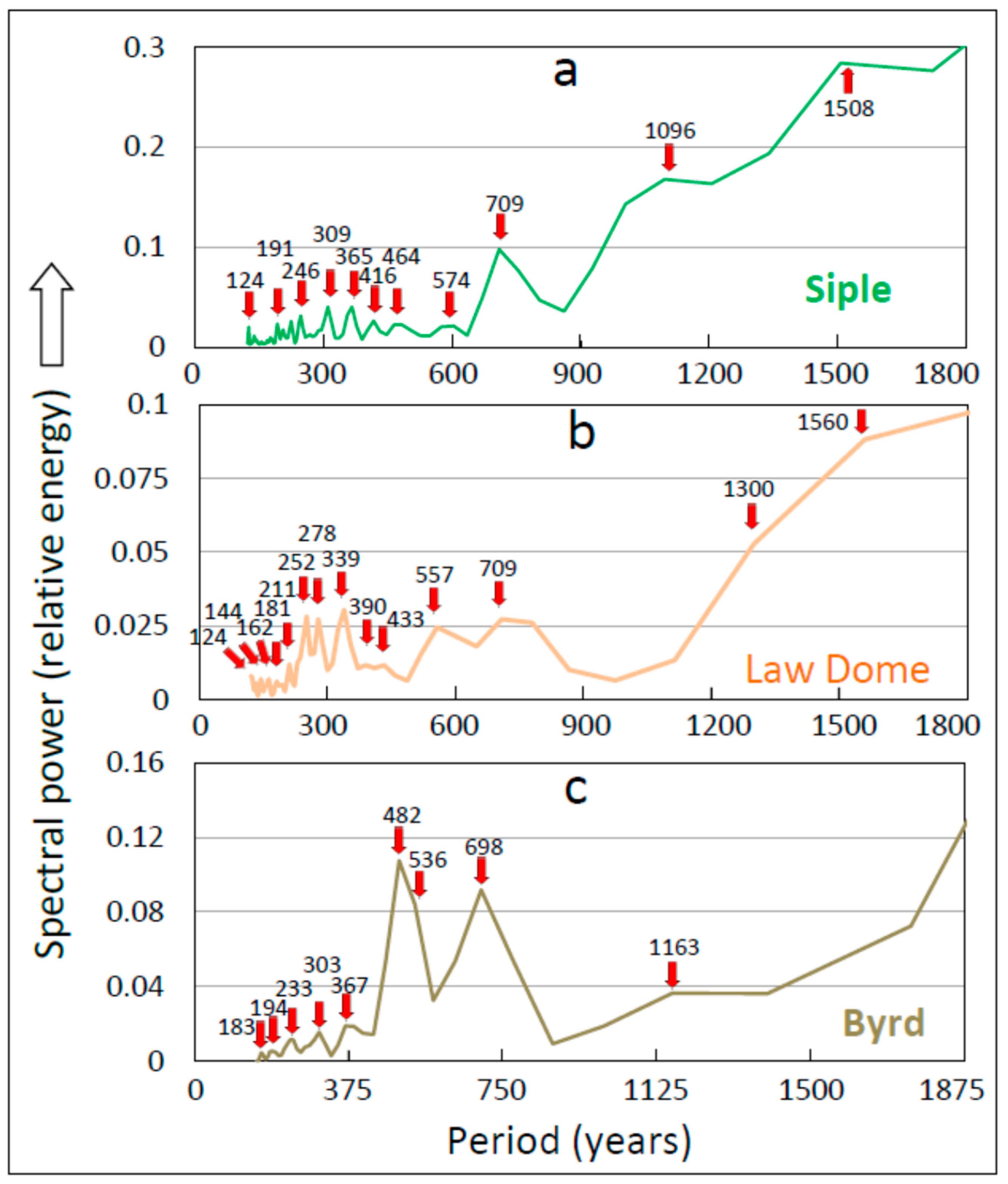
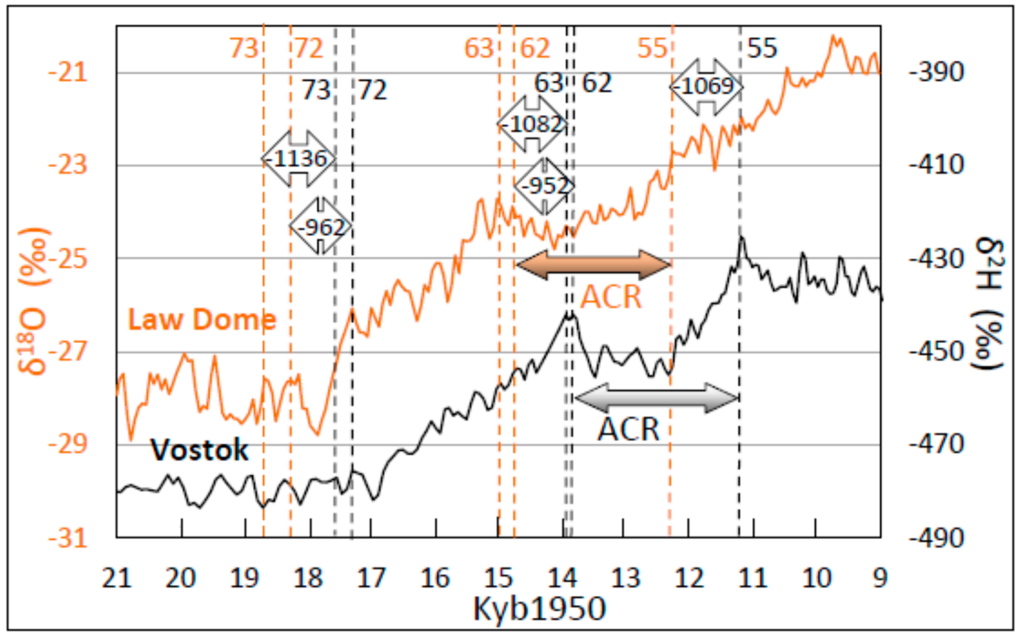
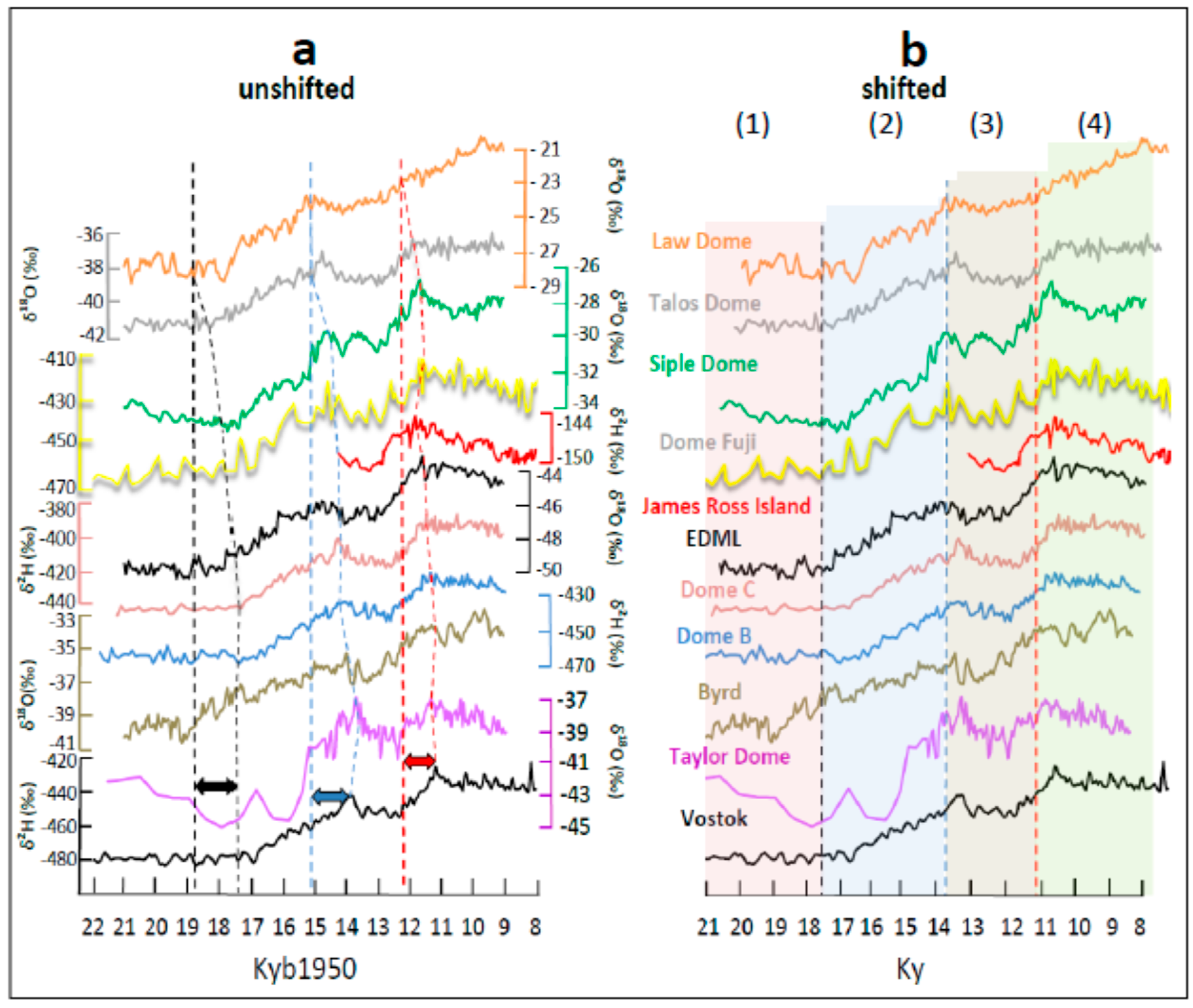
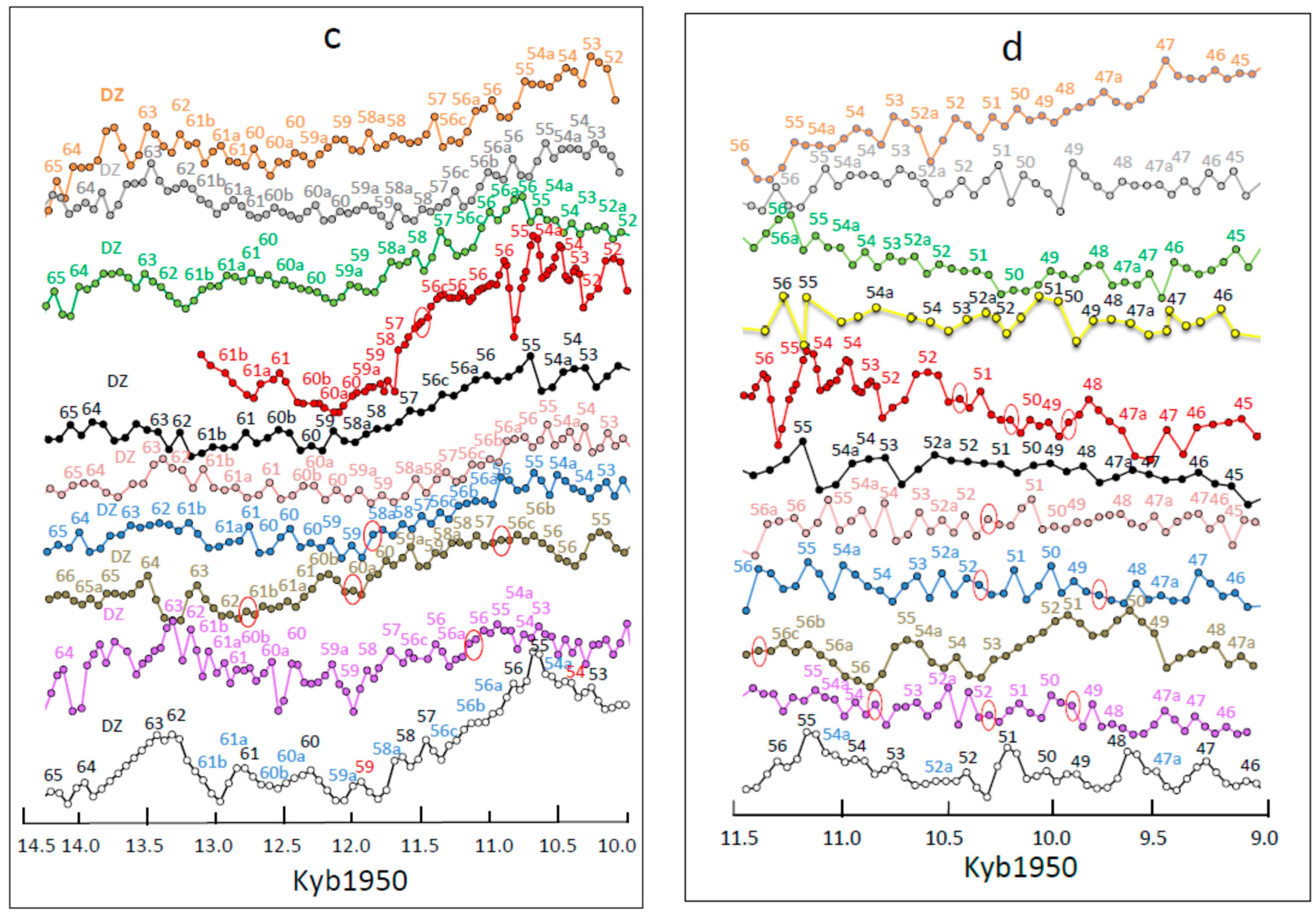
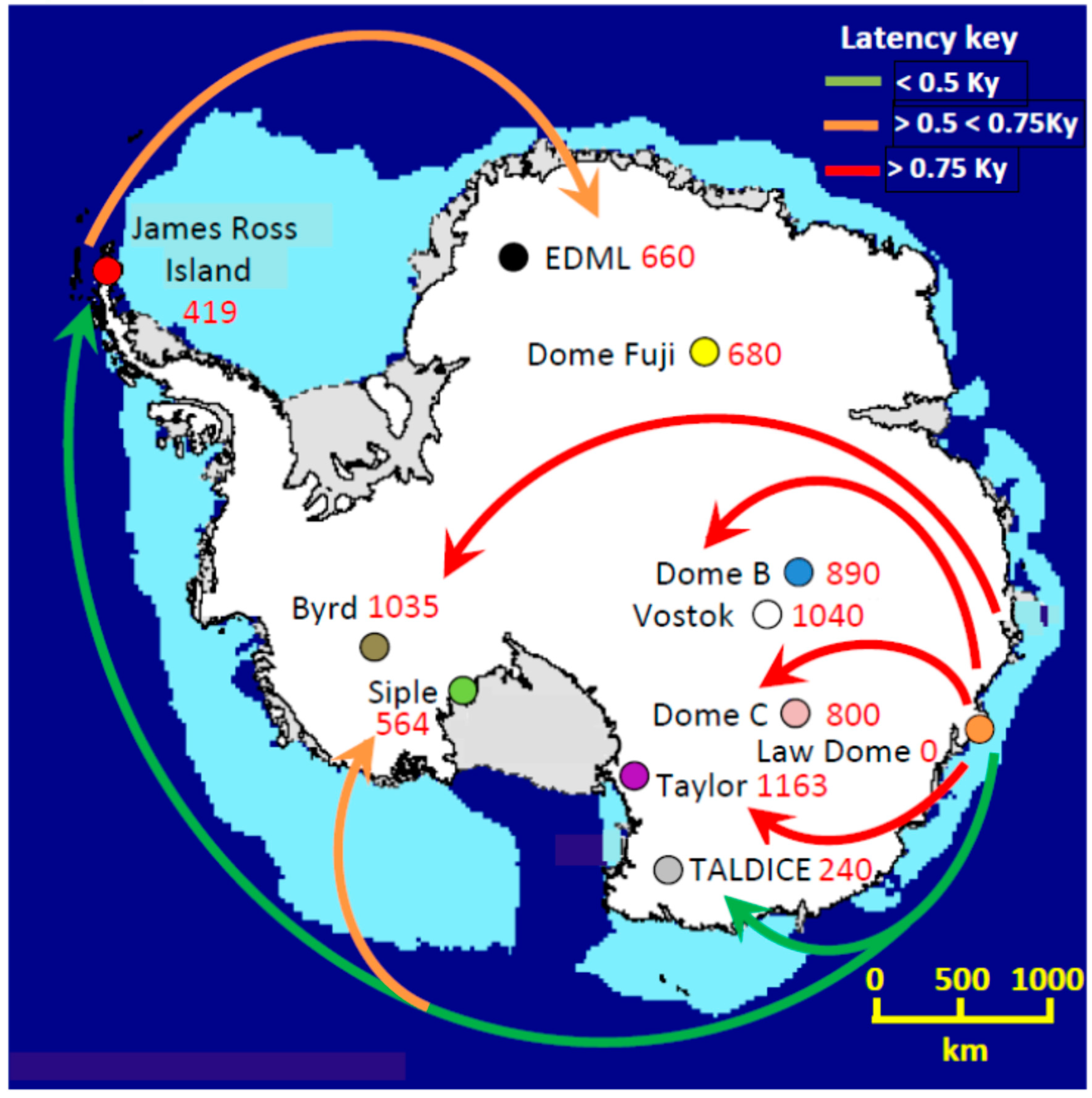
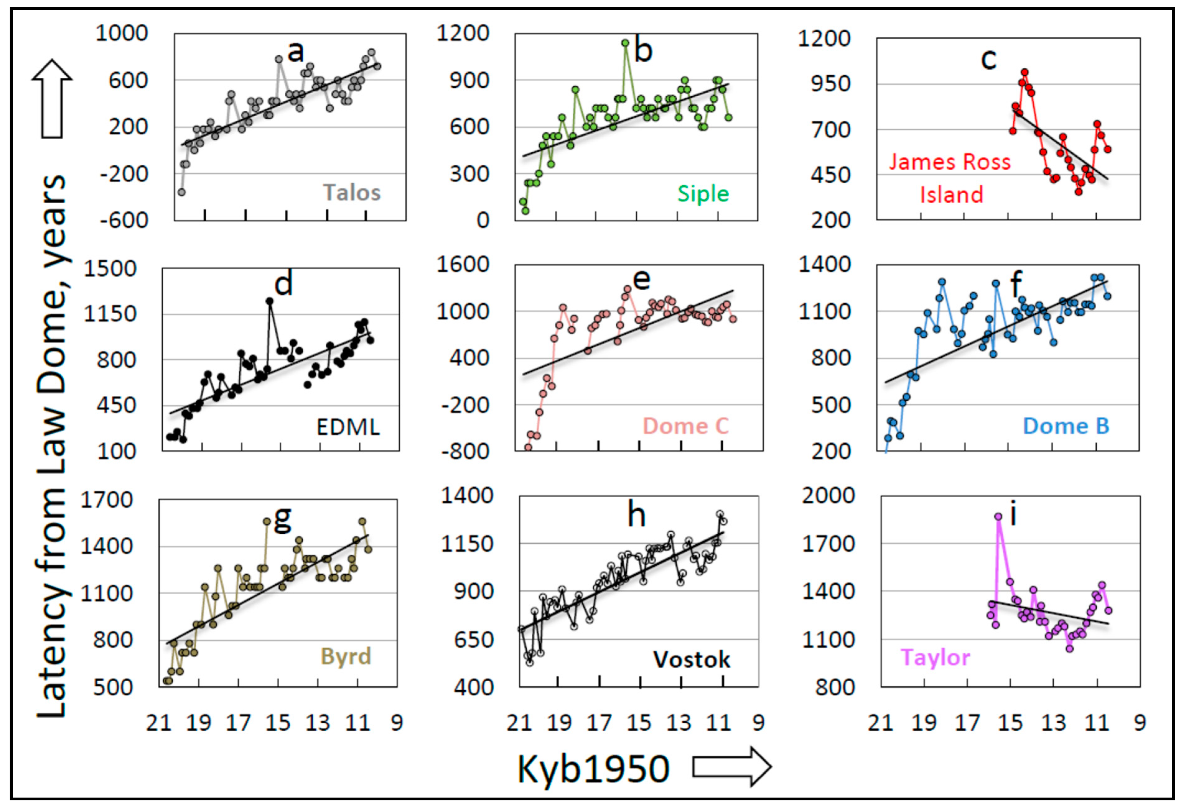
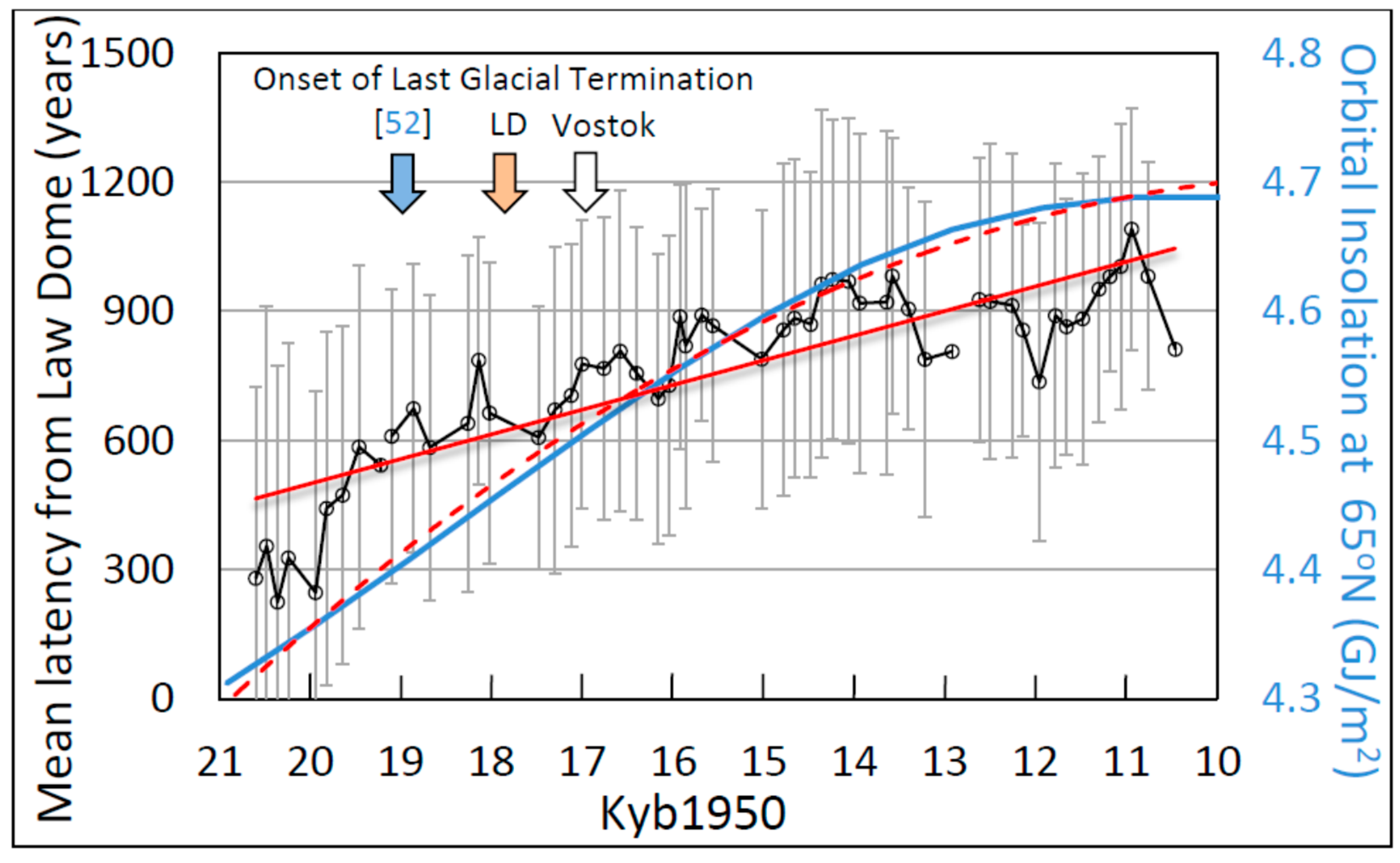
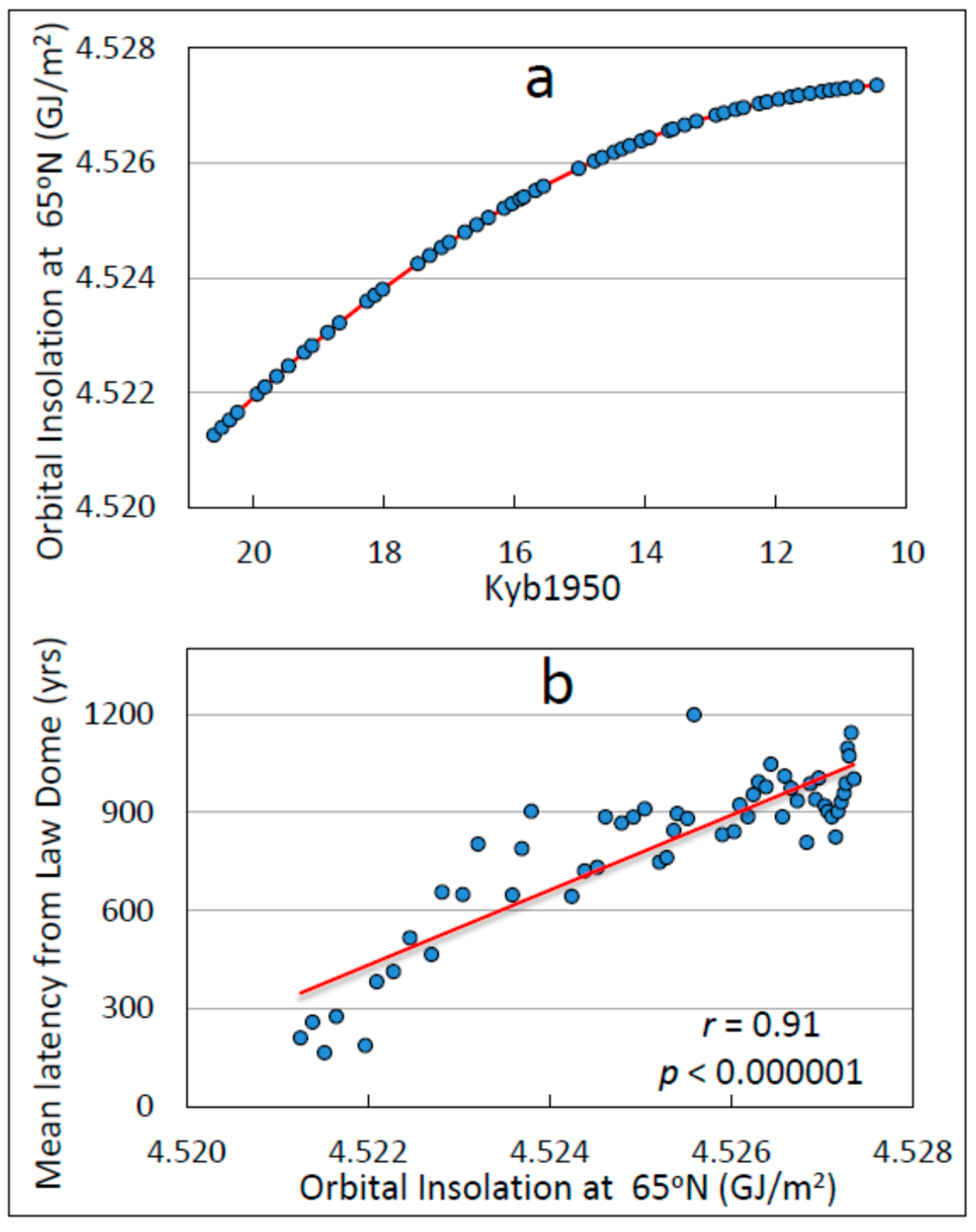
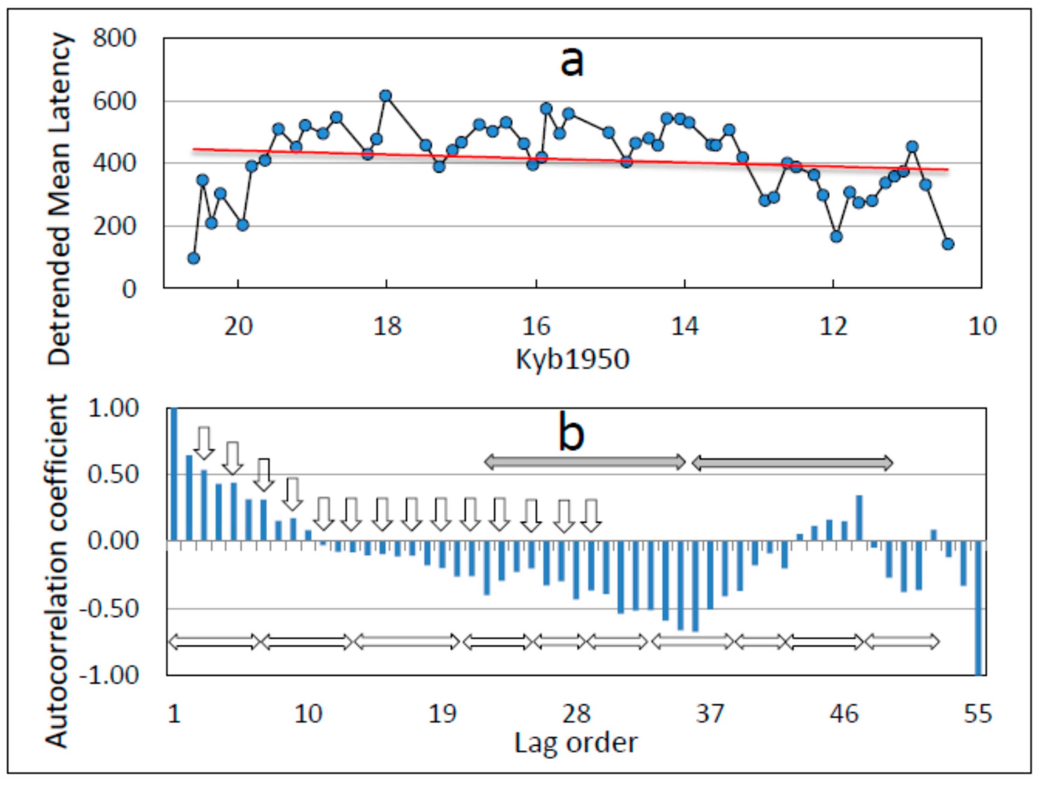
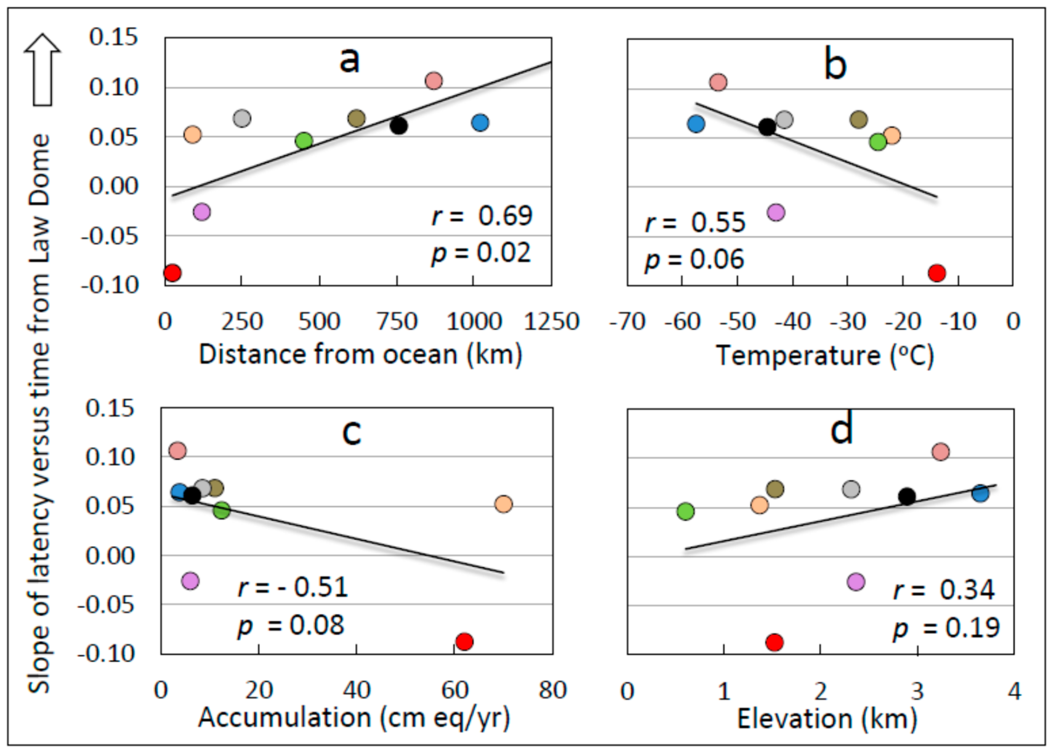
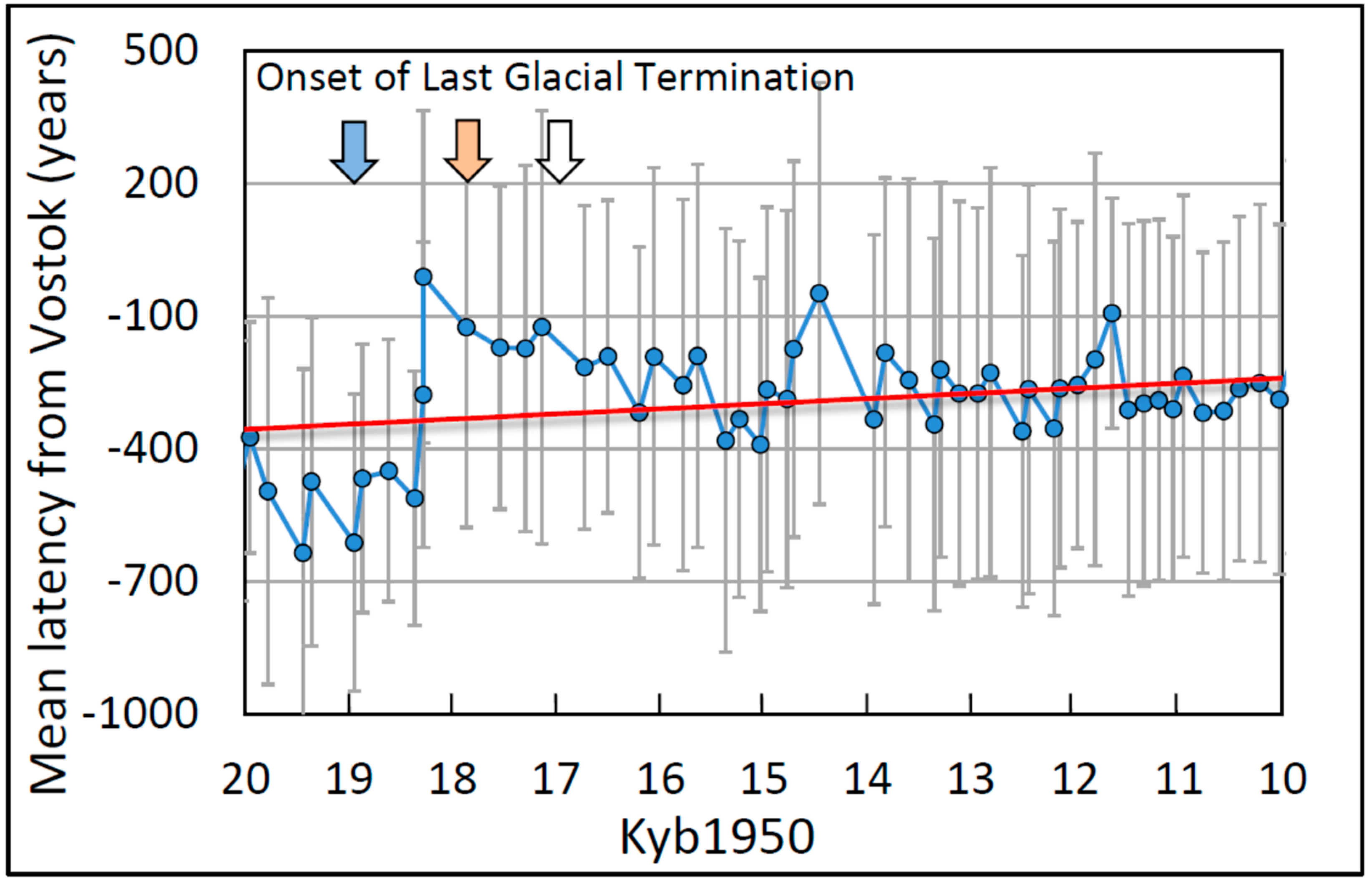
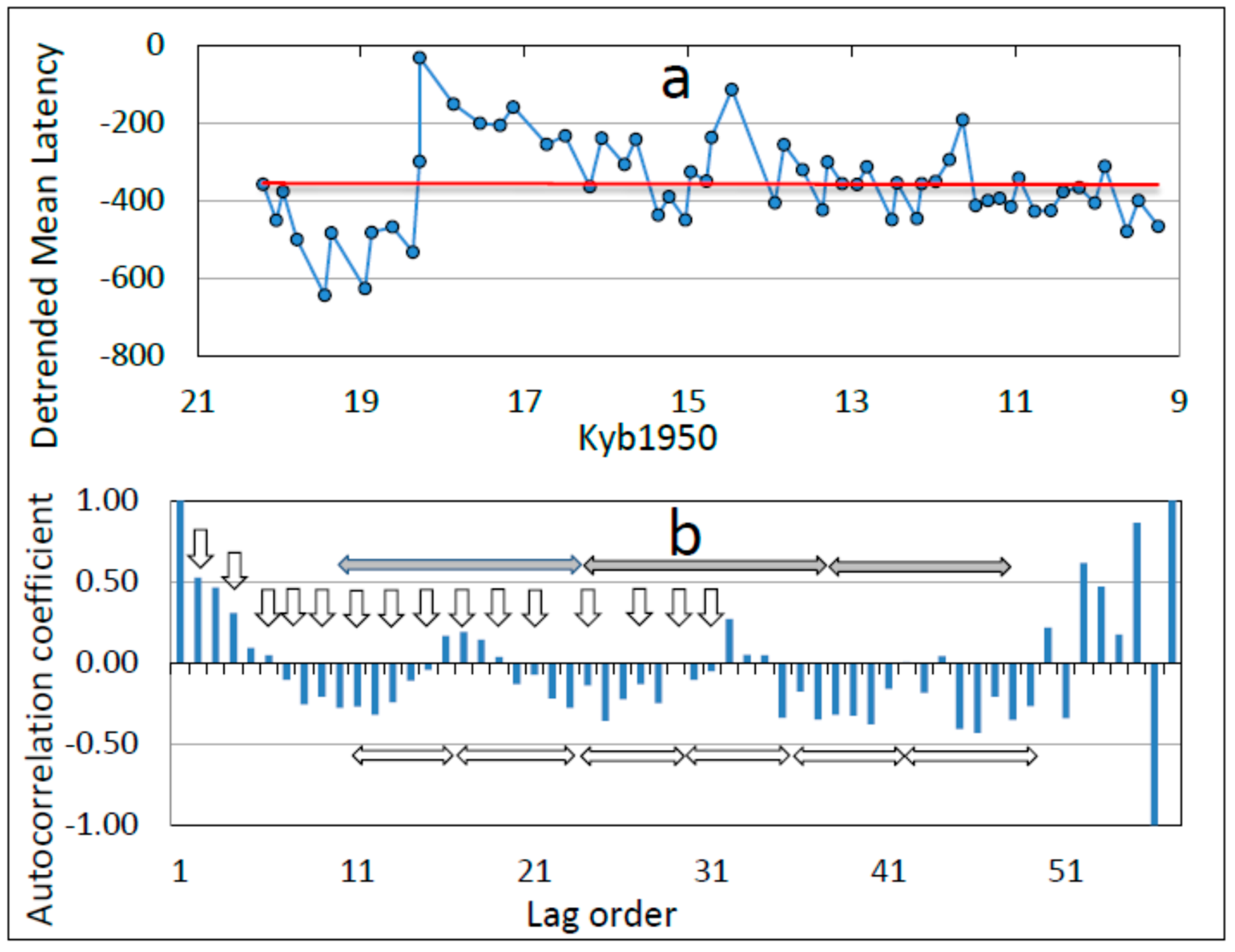
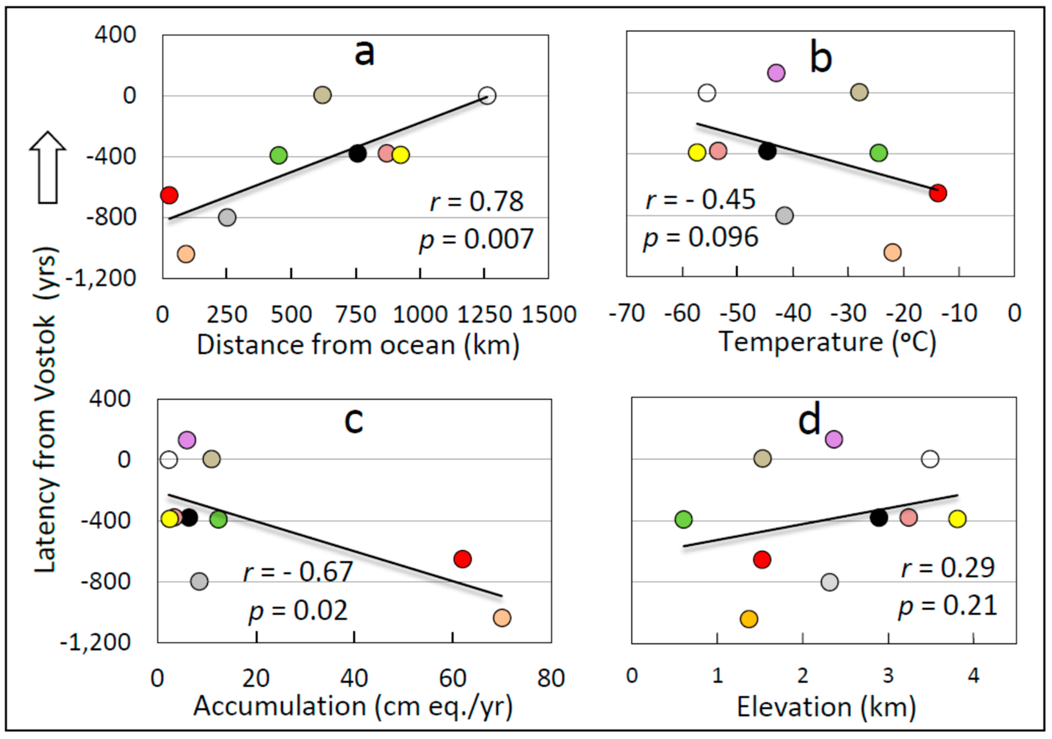
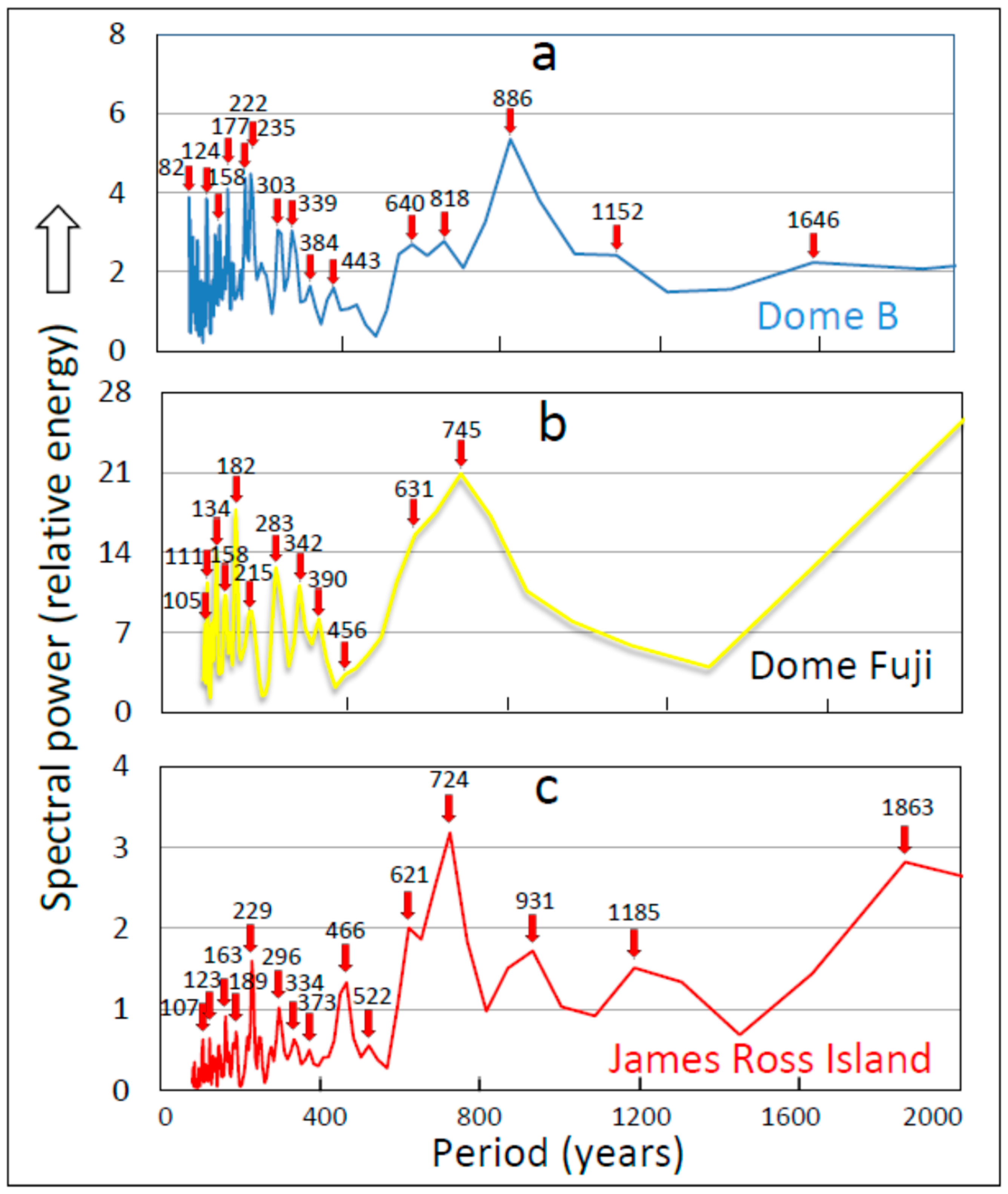
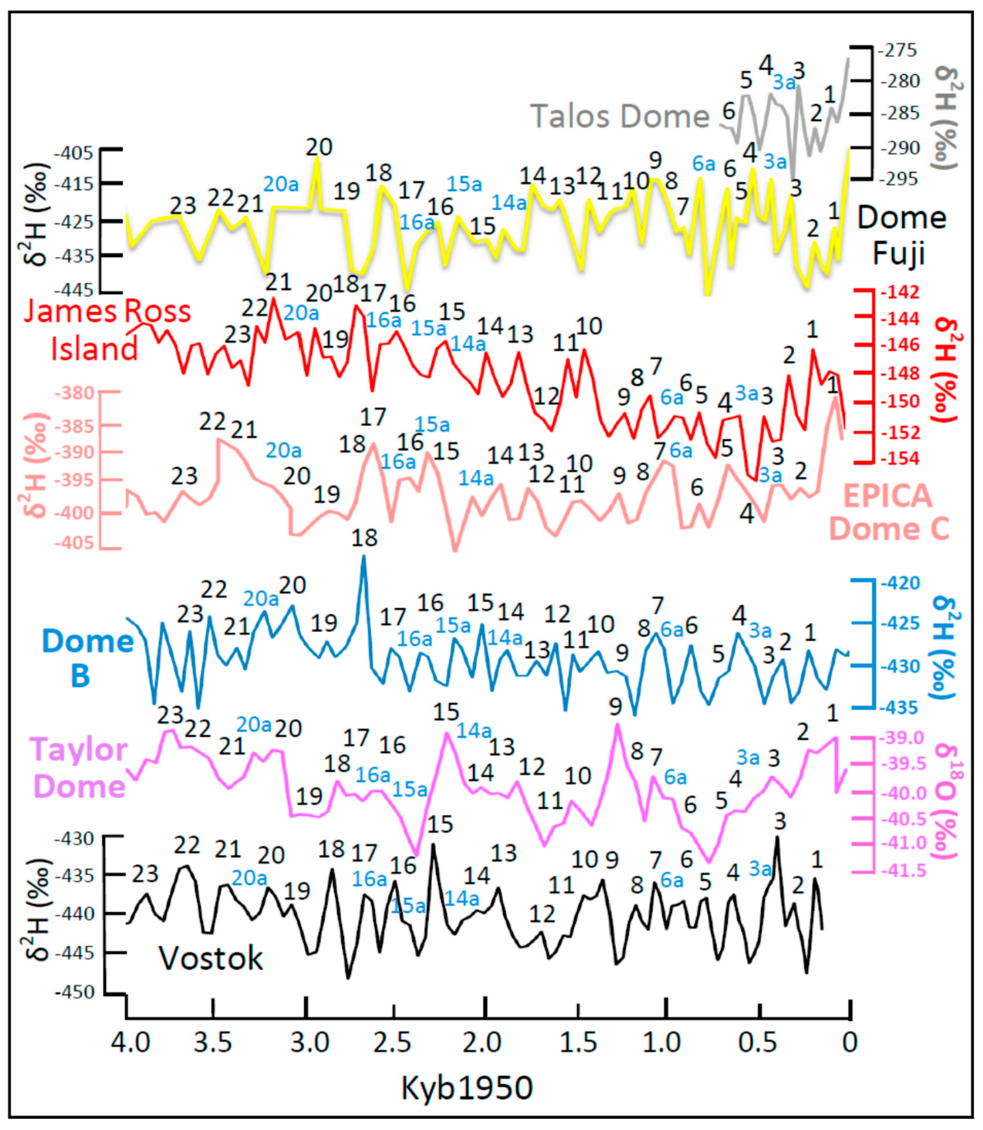
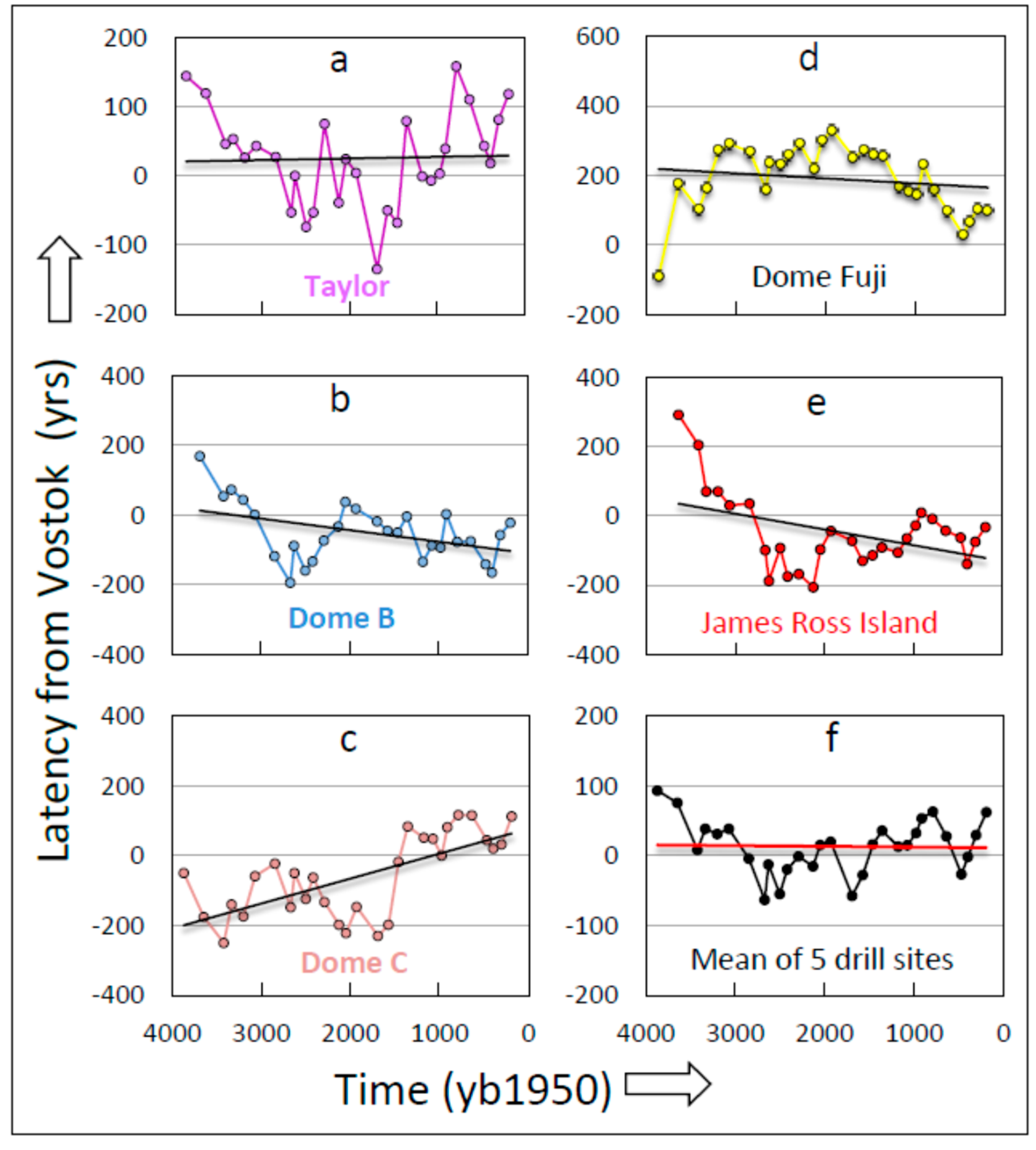
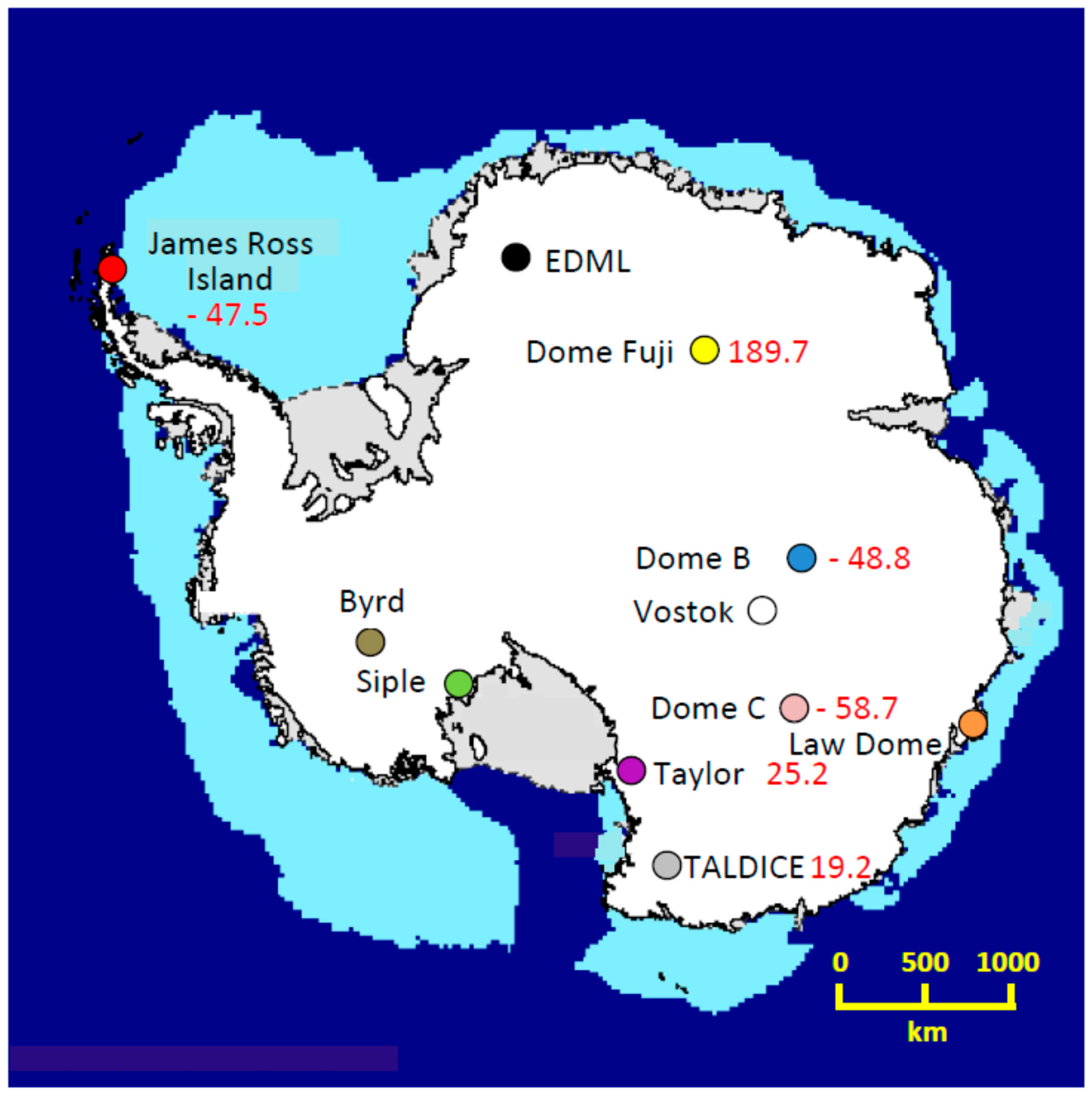
Table 1.
Comparison of climate dynamics of the Antarctic Centennial Oscillation (ACO) with the Antarctic Oscillation (AAO).
Table 1.
Comparison of climate dynamics of the Antarctic Centennial Oscillation (ACO) with the Antarctic Oscillation (AAO).
| 1. Cycle Parameter Correlated with Period | 2. ACO Temperature Proxies ([11], this Paper) | 3. AAO, Patagonia Pollen [88] | 4. AAO, Patagonia Pollen [13] | 5. AAO, Fe in North Atlantic Sediment Core [89] | 6. AAO, Speleotherm δ18O from Ireland [90] | 7. AAO, Falkland Islands Pollen [38] |
|---|---|---|---|---|---|---|
| Amplitude at cycleonset | r = −0.30 p < 0.0001 n = 624 | r = 0.15 p = 0.51 n = 22 | r = 0.03 p = 0.89 n = 24 | r = 0.47 p = 0.02 n = 24 | r = −0.04 p = 0.87 n = 20 | r = 0.21 p = 0.40 n = 18 |
| Cycle amplitude | r = 0.21 p < 0.0001 n = 545 | r = −0.09 p = 0.75 n = 15 | r = 0.51 p = 0.01 n = 24 | r = 0.51 p = 0.01 n = 23 | r = 0.18 p = 0.50 n = 16 | r = 0.44 p = 0.12 n = 14 |
| Cycle symmetry (duration) | r = −0.05 p = 0.48 n = 545 | r = −0.17 p = 0.45 n = 22 | r = −0.09 p = 0.68 n = 24 | r = 0.00 p = 1.0 n = 24 | r = 0.09 p = 0.71 n = 20 | r = −0.14 p = 0.59 n = 17 |
| Cycle symmetry (rate) | r = 0.02 p = 0.48 n = 545 | r = 0.24 p = 0.39 n = 15 | r = 0.03 p = 0.91 n = 17 | r = −0.04 p = 0.87 n = 19 | r = 0.32 p = 0.37 n = 10 | r = −0.50 p = 0.07 n = 14 |
| Warming duration | r = 0.77 p < 0.0001 n = 545 | r = 0.63 p = 0.001 n = 24 | r = 0.35 p = 0.09, n = 24 | r = 0.38 p = 0.07 n = 24 | r = 0.54 p = 0.01 n = 20 | r = 0.69 p = 0.002 n = 18 |
| Cooling duration | r = 0.79 p < 0.0001 n = 545 | r = 0.75 p < 0.0001 n = 24 | r = 0.73 p < 0.0001 n = 24 | r = 0.31 p = 0.14 n = 24 | r = 0.41 p = 0.07 n = 20 | r = 0.73 p = 0.001 n = 18 |
| Warming rate | r = −0.30 p < 0.0001 n = 545 | r = −0.40 p = 0.11 n = 18 | r = 0.02 p = 0.93 n = 24 | r = 0.10 p = 0.70 n = 17 | r = 0.21 p = 0.44 n = 16 | r = 0.004 p = 1.00 n = 14 |
| Cooling rate | r = −0.20 p < 0.0001 n = 545 | r = −0.50 p = 0.04 n = 17 | r = −0.04 p = 0.85 n = 24 | r = −0.03 p = 0.91 n = 18 | r = 0.17 p = 0.53 n = 16 | r = 0.27 p = 0.35 n = 14 |
Shown are Pearson correlation coefficients (r) between cycle period and other major cycle parameters (column 1) for the Antarctic Centennial Oscillation (ACO) (column 2) and for the AAO (columns 3–7). The top row shows the cycle identity, location, proxy used, and source of data. The red font within cells designates correlation coefficients that are discernibly different from zero (p < 0.05) or show a tendency toward a discernible difference from zero (0.05 < p < 0.01). Black font designates correlation coefficients that are not discernibly different from zero. Both correlations and the absence of correlation of key cycle properties with period are generally comparable across paleoclimate cycles for the ACO and AAO, suggesting that they are different manifestations of the same natural climate cycle. Use of the non-parametric (distribution-free) Spearman Rho correlation coefficient yielded similar and stronger conclusions (not shown). Abbreviations: Amplit., amplitude; dur., duration; n, sample size; p, alpha level (probability of Type I error); r, Pearson product moment correlation coefficient.
Table 2.
Comparison of key cycle properties (period, duration symmetry, rate of temperature change symmetry) of the Antarctic Centennial Oscillation (ACO, black font) with homologous properties of the Antarctic Oscillation (AAO, purple font) using a two-sided t-test.
Table 2.
Comparison of key cycle properties (period, duration symmetry, rate of temperature change symmetry) of the Antarctic Centennial Oscillation (ACO, black font) with homologous properties of the Antarctic Oscillation (AAO, purple font) using a two-sided t-test.
| 1. Cycles Compared, AAO Location, AAO Proxy, References | 2. Mean Periods of Cycles (y) | 3. Mean Duration Symmetries (Warming/Cooling) | 4. Mean Rate Symmetries (Warming/Cooling) |
|---|---|---|---|
| ACO v. AAO, Patagonia, pollen [88] | 145 (n = 21) 137 (n = 22) p = 0.70 | 1.36 (n = 22) 0.84 (n = 14) p = 0.79 | 1.26 (n = 23) 1.58 (n = 14) p = 0.39 |
| ACO v. AAO, Patagonia, pollen [13,88] | 144 (n = 24) 120 (n = 24) p = 0.12 | 1.33 (n = 23) 1.27 (n = 24) p = 0.83 | 1.00 (n = 22) 1.39 (n = 23) p = 0.27 |
| ACO v. AAO, NA, Fe in Sediment Core, [13,89] | 118 (n = 16) 107 (n = 24) p = 0.40 | 1.33 (n = 26) 1.26 (n = 24) p = 0.76 | 1.00 (n = 22) 1.75 (n = 20) p = 0.32 |
| ACO v. AAO, δ18O in in Irish speleotherm [13,90] | 144 (n = 24) 146 (n = 20) p = 0.93 | 1.33 (n = 23) 1.25 (n = 20) p = 0.81 | 1.00 (n = 22) 0.66 (n = 13) p = 0.17 |
| ACO v. AAO, Falkland Islands, pollen [38] | 143 (n = 18) 132 (n = 18) p = 0.49 | 1.42 (n = 18) 1.06 (n = 18) p = 0.20 | 1.26 (n = 18) 1.19 (n = 14) p = 0.88 |
Shown are the mean values of three key cycle properties (column 2, repetition period; column 3, symmetry of cycle duration; and column 4, symmetry of cycle rate of temperature change) for the Antarctic Centennial Oscillation (ACO) v. the Antarctic Oscillation (AAO) over comparable time periods. Each cell contains three entries: the mean value of the ACO computed from paleoclimate data (stable isotopes in ice cores, black font), the homologous mean for the AAO over the same time period computed from contemporary climate data (purple font), and the probability that the two means are discernibly different (red font). The red font identifies the alpha level returned from a two-sided heteroscedastic t-test comparing the two means in each cell. The differences between means in each cell are in all cases statistically indiscernible (p > 0.05), consistent with the hypothesis that the ACO and the AAO are the same natural climate cycle. Abbreviations: δ18O, oxygen stable water isotope; Fe, iron; NA, North Atlantic; n, sample size; p, alpha level; v., versus.
© 2019 by the authors. Licensee MDPI, Basel, Switzerland. This article is an open access article distributed under the terms and conditions of the Creative Commons Attribution (CC BY) license (http://creativecommons.org/licenses/by/4.0/).
Share and Cite
MDPI and ACS Style
Davis, W.J.; Taylor, P.J.; Davis, W.B. The Origin and Propagation of the Antarctic Centennial Oscillation. Climate 2019, 7, 112. https://0-doi-org.brum.beds.ac.uk/10.3390/cli7090112
AMA Style
Davis WJ, Taylor PJ, Davis WB. The Origin and Propagation of the Antarctic Centennial Oscillation. Climate. 2019; 7(9):112. https://0-doi-org.brum.beds.ac.uk/10.3390/cli7090112
Chicago/Turabian StyleDavis, W. Jackson, Peter J. Taylor, and W. Barton Davis. 2019. "The Origin and Propagation of the Antarctic Centennial Oscillation" Climate 7, no. 9: 112. https://0-doi-org.brum.beds.ac.uk/10.3390/cli7090112
Note that from the first issue of 2016, this journal uses article numbers instead of page numbers. See further details here.