Hydrological Modeling Response to Climate Model Spatial Analysis of a South Eastern Europe International Basin


1
Department of Civil Engineering, Aristotle University of Thessaloniki, 54124 Thessaloniki, Greece
2
Department of Meteorology Climatology, School of Geology, Aristotle University of Thessaloniki, 54124 Thessaloniki, Greece
*
Author to whom correspondence should be addressed.
Climate 2020, 8(1), 1; https://0-doi-org.brum.beds.ac.uk/10.3390/cli8010001
Submission received: 24 October 2019
/
Revised: 5 December 2019
/
Accepted: 18 December 2019
/
Published: 19 December 2019
(This article belongs to the Special Issue Impact of Climate-Change on Water Resources)
Abstract
:One of the most common questions in hydrological modeling addresses the issue of input data resolution. Is the spatial analysis of the meteorological/climatological data adequate to ensure the description of simulated phenomena, e.g., the discharges in rainfall–runoff models at the river basin scale, to a sufficient degree? The aim of the proposed research was to answer this specific question by investigating the response of a spatially distributed hydrological model to climatic inputs of various spatial resolution. In particular, ERA-Interim gridded precipitation and temperature datasets of low, medium, and high resolution, i.e., 0.50° × 0.50°, 0.25° × 0.25°, and 0.125° × 0.125°, respectively, were used to feed a distributed hydrological model that was applied to a transboundary river basin in the Balkan Peninsula, while all the other model’s parameters were maintained the same at each simulation run. The outputs demonstrate that, for the extent of the specific basin study, the simulated discharges were adequately correlated with the observed ones, with the marginally best results presented in the case of precipitation and temperature of 0.25° × 0.25° spatial analysis. The results of the research indicate that the selection of ERA-Interim data can indeed improve or facilitate the researcher’s outputs when dealing with regional hydrologic simulations.
1. Introduction
The accuracy of hydrologic models is limited by many factors [1,2]. Data availability, both in terms of quantity, i.e., large data series and spatial coverage of the case study basin, and quality, i.e., reliable and unbiased datasets, plays a significant role in the modeling procedure and is one of the factors that are bound to affect the produced results. O’Riordan [3] demonstrated that the lack of historic data or even the comprehensiveness of monitoring could lead to distorted findings. In hydrological simulations and forecasting, precipitation is one of the most important inputs, with the precipitation’s gauge network density and the gauges’ spatial distribution having direct impacts on the modeling results [4]. Xu et al. [5] showed that the error of the simulated runoff was gradually narrowed to a specific threshold number of gauges, beyond which the model’s performance did not demonstrate considerable improvements. Similarly, Anctil et al. [6] demonstrated that a model’s performance was reduced when spatial rainfall was derived from a network where the number of network gauges was lower than a specific threshold. Woods et al. [7] found that the size of the representative elementary area [8] was influenced more by the catchment topography than by the spatial resolution of the rainfall data. Moreover, the density of the stations/grids for a hydrologic network that was defined by the World Meteorological Organization [9] indicated that the density was strongly dependent on the physiographic characteristics of the regions. The current availability of gridded precipitation data series [10,11,12] offers spatial coverage at various resolutions on a worldwide scale.
The accuracy of gridded data sources was thoroughly examined in the literature [13,14,15,16]. In northeast China, for example, a comparative study regarding gridded datasets, such as those of the Global Precipitation Climatology Center (GPCC), the Climate Research Unit (CRU), and the University of Delaware (UDEL), with station-based precipitation data, demonstrated that gridded databases overestimated the annual precipitation [17]. At the European scale, the comparison of existing precipitation datasets with E-OBS gridded data revealed that the differences were relatively large, and usually biased toward lower values in E-OBS [18]. Nevertheless, the selection of the proper grid resolution is of particular significance, since low grid resolution could lead to uncertainty of the predictions, while, in the case of overestimation of resolution, the workload is increasingly demanding [19]. Gridded climatic variables were also exploited for the assessment of other atmospheric processes, such as the daily global solar radiation [20].
Meteorological reanalysis data are among the most used gridded datasets, with those most widely used presented by Fuka et al. [21]. Although both gridded data and reanalysis data initially come from terrestrial and airborne observation networks, the reanalysis data go a step forward, i.e., they are assimilated into a numerical weather prediction model to produce a spatially and temporally coherent synthesis of meteorological variables covering the last few decades [22]. Reanalysis provides a multivariate, spatially complete, and coherent record of the global atmospheric circulation [23], and its usefulness was proven both in areas where there is a plethora of data and in areas where weather stations are limited or even do not exist [24]. Many studies compared reanalysis products to observation data and, in general, they concluded that reanalysis products are comparable to station measurements [23,25,26]. ERA-Interim is one of the latest global reanalysis products developed by the European Center for Medium-Range Weather Forecasts (ECMWF) [23]. ERA-Interim is highly used over regions with sparse observations, such as high mountainous regions or complex terrains [27,28]. The accuracy of these datasets was evaluated in many places of the word. For example, the Hu et al. [29] investigation regarding the reliability of the precipitation variable took place in central Asia. ERA-Interim was also used to assess, in terms of consistency, the temperature and precipitation extremes [30].
One of the principal hydro-climate applications of gridded datasets is to incorporate them into spatially distributed hydrologic models as climate forcings [31]. The literature presents some recent studies that investigated the impact of the spatial resolution of reanalysis products on hydrologic modeling [32,33]. In a large mountain watershed in Canada, for example, Woo and Thorne [34] exploited ERA-40, NCEP–NCAR, and NARR reanalysis products to simulate the contribution of snowmelt to the river regime. However, coupling of reanalysis data with hydrologic models was less explored and, in general, studies on this topic focused on a limited number of basins [22]. Moreover, the literature review showed that the coupling of reanalysis data with hydrologic models is mainly based on single spatial resolutions [35,36]. Fuka et al. [21], for example, in their hydrologic simulation, used specific reanalysis products covering the globe at hourly time steps since 1979 at a 38-km resolution. Limited researches evaluated a broader range of spatial analysis, such as Essou et al. [22], where they used three different reanalysis datasets of spatial resolution varying between 30 km and 10 km to trigger the hydrologic simulation procedure.
Based on the aforementioned review, this specific research aims at investigating the runoff response of a watershed in reanalysis climatic data of varying resolution. In particular, this study seeks to assess the sensitivity of a hydrologic model, namely MODSUR, by comparing the low-resolution ERA-Interim datasets (0.50° × 0.50°) with the medium-resolution ERA-Interim datasets (0.25° × 0.25°) and the high-resolution ERA-Interim datasets (0.125° × 0.125°). The case study area is a transboundary river basin in southeastern Europe (SEE), where the climatic conditions in the upstream part of the basin are different to those of the downstream part due to its proximity to the sea. The performed analysis on the three different datasets demonstrated the degree of correlation among the relevant climatic variables, as well as the correlation of the simulated discharges with the observed discharges of the river. This research is considered of significant importance because ERA-Interim reanalysis data are routinely used for (i) case areas where the lack of data is dominant, and (ii) the bias correction of climatic variables, when climate change is inserted into the research. Hence, the outputs could shed light on questions relative to the required resolution of climatic data when used in hydrologic studies.
2. Materials and Methods
2.1. Case Study Area
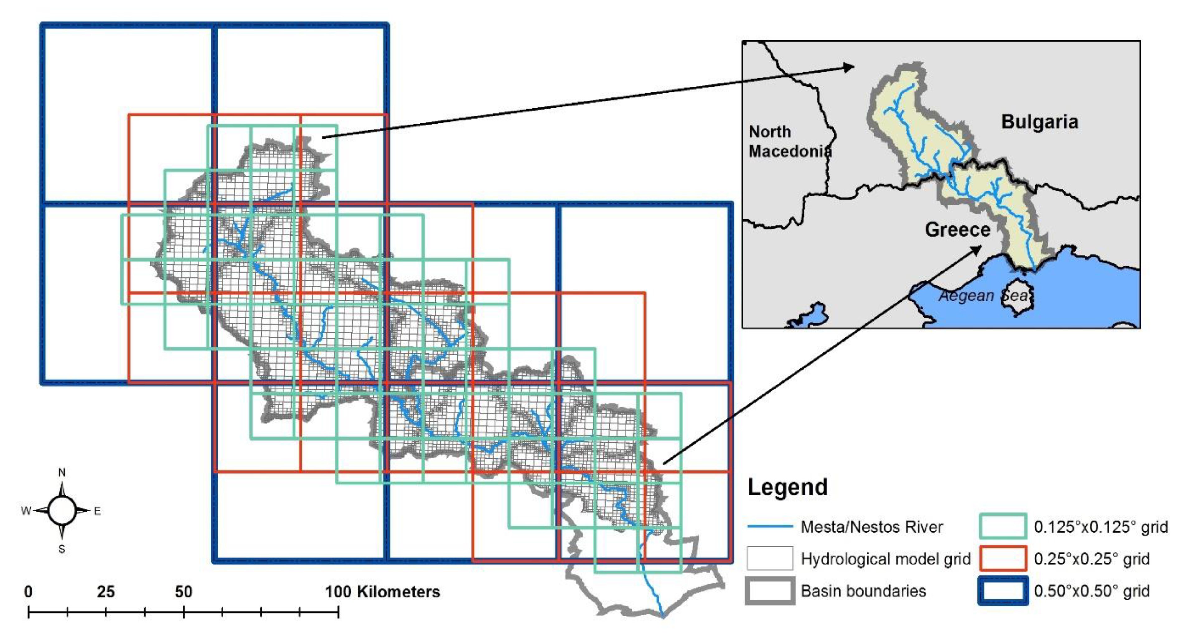
The transboundary basin of Mesta/Nestos River, which is shared between Bulgaria and Greece, was the area of interest in this research. The specific basin is one of the 18 international rivers and lake basins in southeastern Europe and one of the five transboundary river basins of Greece. Moreover, this basin forms part of the Hydrology for the Environment, Life and Policy (HELP) demonstration basins of UNESCO’s Intergovernmental Hydrological Programme (IHP) [37]. The morphology of the catchment is mountainous with the exception of the delta region (Figure 1). Due to the basin’s (i) orientation from north to south and (ii) complex topography, since it spreads among the highest mountains of SEE and the sea level, the climate can change from typically coastal Mediterranean to practically alpine [38].
The headwaters are located in southwestern Bulgaria, while the river outlets are located in the north Aegean Sea, in Greece. The total length of the river’s main course and the basin’s extent are 255.0 km and 6,218.0 km2, respectively, figures that are almost equally shared by the two countries (Figure 1). The average inflows into Greece are estimated at 0.14 × 10⁹ m3, i.e., water volumes that are significantly lower (approximately 50%) than the 0.278 × 10⁹ m3 that are referred to in the Water Convention [39]. The observed decrease in water inflows from the upstream country to the downstream country are mainly attributed to the climatic variations. Bulgaria, in particular, argues [39] that, over the last 20 years, precipitation presented a decrease of 30%, thus leading to a subsequent decrease in water discharge.
2.2. Reanalyis Data and Derived Datasets
The analyzed data consisted of temperature and precipitation time series obtained from ERA-Interim, produced by the ECMWF (European Center for Medium-Range Weather Forecasts). Detailed information about the ERA-Interim reanalysis can be found in Dee et al. [23]. The precipitation data used in this study were projected on a grid of 0.5° × 0.5° (ERAI_50), 0.25° × 0.25° (ERAI_25), and 0.125° × 0.125° (ERAI_12.5) from the original Gaussian reduced grid (T255 reduced Gaussian grid of about 0.7° × 0.7°) [40], and they are provided at a daily time step. The length of the time series was 35 years extending from 1981 to 2015, with the specific length considered sufficient to carry out statistical analysis of the climatic data. ERA-Interim is an improved version compared to previous reanalysis products of ECMWF, based on the use of additional observations, the updated data assimilation system, and the increased resolution [23].
2.3. River Basin Simulation
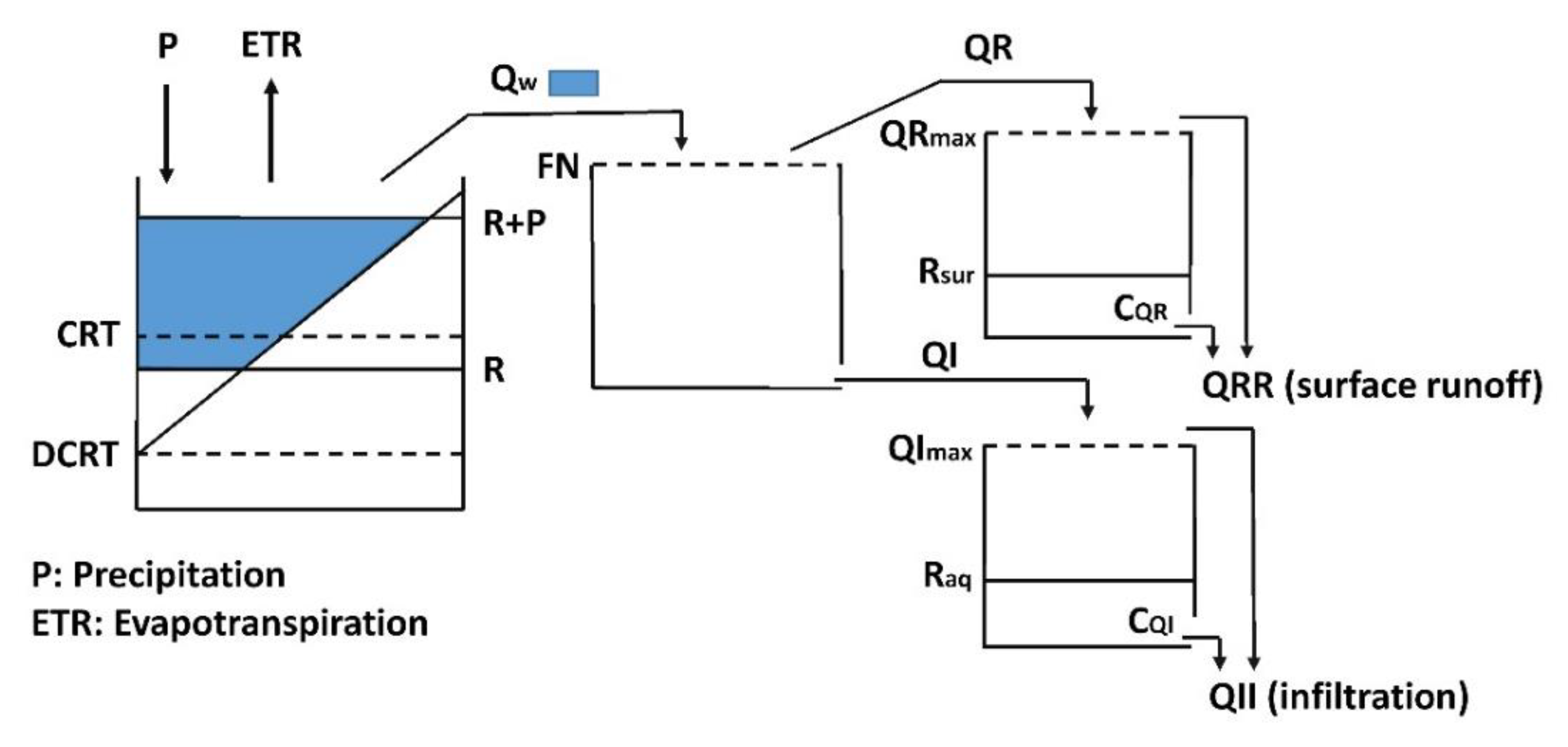
The simulation of the basin’s discharges was accomplished with the MODSUR (modélisation de transfers de surface) spatial distributed hydrologic model. MODSUR is the surface modeling component of the coupled surface and groundwater MODCOU (modélisation couplée) simulation model, which was developed by the Ecole Nationale Supérieure des Mines de Paris [41]. The model operation is based on a densely spaced grid, and it uses a progressive quadtree structure with varying cell sizes. This means that the surface domain is divided into grid cells of size a, 2a, 4a, and 8a, with the higher resolution attributed to the grid cells representing the river. For the selected case study basin, the utilized grid was composed of 9212 cells. The ensemble of connected cells builds the runoff network, which gathers the flow down to the catchment outlet. The water budget in the model was computed in each grid cell using a system of four reservoirs [41,42], as a function of precipitation (P), evapotranspiration (ETR), and water level of the reservoir (R), i.e., the initial stocked water in the soil. The system of reservoirs is responsible for the repartition of rainfall water into runoff, infiltration, evapotranspiration, and soil water storage (Figure 2).
The excess water transferred from the first to the second reservoir is defined as follows:
where DCRT is the minimum stocked water (mm) in the soil below which no water quantity is available, and CRT the average stocked water quantity (mm), while Rmax, RBA, and dR are expressed as follows:
The partitioning of the water to runoff (QR) and infiltration (QI) is conducted in the second reservoir. It is controlled by the parameter FN that corresponds to the maximum value of infiltration over a time step (mm/day), and it is expressed as follows:
The third and fourth reservoirs are responsible for the calculation of the final infiltration (QII) and the surface runoff (QRR). The latter is further analyzed as pure runoff (if overflowing) and delayed runoff. The final calculation of the QRR is given as follows:
where Rsur is the level of the surface runoff reservoir (mm), QRmax the surface runoff reservoir’s overflow level (mm), and CQR is the depletion ratio of the surface runoff reservoir (mm). The operation of the infiltration reservoir is similar to the aforementioned reservoir. For the specific case study, no interactions between the surface domain and the water table were introduced due to lack of data. Thus, the infiltration reservoir was not inserted in the simulation process.
For the Mesta/Nestos basin, the reservoir parameters were based on the catchment characteristics with digitized maps of geology and land uses to be overlaid on the hydrologic grid. For each cell of the grid, the dominant characteristics, e.g., geological formations and land-use types, were selected to define the relevant infiltration and evapotranspiration coefficients per cell. The MODSUR model was implemented in basins of varying scales, e.g., the Maritza basin in Bulgaria [43], as well as the selected case study [37].
Because of the increased altimetry of the basin, as the highest peak of the Balkan Peninsula (namely, peak Musala of 2925 m above sea level) is located within the basin, the snow coverage and melting processes play a significant role both in the river’s spring increased discharge and in the continuity of the discharge during the summer. The snow component NEIGE, which is a compatible add-on of the MODSUR model, was used to simulate the snow cover regime on the principle of “degree days” [44,45], using an approach which distinguishes snow melting processes between forested and non-forested areas. The degree-day method is a temperature index method that equates the total daily melt to a coefficient times the temperature difference between the mean daily temperature and a base temperature (generally 0 °C).
where M is the snowmelt expressed in mm/day, CM is the degree-day coefficient (mm/degree-day °C), and Ta and Tb are the mean daily air and base temperatures (°C), respectively. The coefficient CM depends on the season and the location, and it varies between 1.6 and 6.0 mm/degree-day °C [45].
In the NEIGE model [46], the snowmelt process is conditioned by the following equation:
where tsto is the temperature of the stocked snow (°C), cof is a coefficient of warming of the stocked snow, tmean is the average daily air temperature (°C), and ts is the threshold temperature for the snow melting (°C).
If this first condition is verified, then a portion of the stocked snow layer could be melted. However, the stocked snow layer has a specific storage capacity of liquid water. In order for the water to be outflowed, the volume of the stocked water should exceed that storage capacity, with the latter expressed as follows:
where Snt is the water (in liquid form) accumulated in the stocked snow layer (mm), ttf is the percentage of transformation (mm/°C), Sts is the threshold temperature for the transformation (°C), and Sn is the stocked snow (mm). When the previous conditions are coupled, then the quantity, Fn(j), of the melted snow in mm is given as follows:
For the case study basin, the parameters of the NEIGE model, such as the threshold temperatures in °C for the snow melting in the forested and non-forested areas, were retrieved by Etchevers and Martin [47]. The variables proposed by the aforementioned authors were used by the French Meteorological Organization in their snow melt model for a Mediterranean basin, i.e., a basin which has similar characteristics to the current case study.
As aforementioned, the MODSUR model was already successfully applied to the study area, with the calibration and validation period from 1987 to 1993 (R2 = 0.64) and from 1994 to 1995 (R2 = 0.68), respectively [37]. For the model calibration, the precipitation data came from a network of 18 stations covering both parts of the basin, while the measured discharges were derived from two gauge stations. Although the rainfall datasets were available at a daily time step, the time step of the historical discharges was at the monthly level. For that purpose, the daily simulated outputs of the hydrologic model were averaged at monthly mean values in order to perform the model validation. In the present research, the parameterization of the model was the same as the aforementioned one [37], and the modifications were related to the forcing variables. Daily precipitation and temperature came from the three different climatic datasets, one per climate model, and they covered a period of 15 years, i.e., from 1 January 1981 to 31 December 1995. The potential evapotranspiration (PET) was calculated based on the Thornthwaite method utilizing the temperature time series of each dataset. The climatic gridded variables were nested in the hydrologic model grid with the use of Geographic Information Systems’ (GIS) spatial analyst tools. Finally, in order to perform a comparison with the historical monthly observations, the simulated daily discharges for each one of the ERA-Interim datasets were aggregated at monthly level. It should also be stated that the simulated flows using different ERA-Interim resolution datasets were conducted on a 15-year period (1981–1995) that included the nine-year calibration validation period (1987–1995) of the hydrologic model.
The evaluation of the model’s results was conducted with the coefficient of determination (R2), which describes the degree of collinearity between simulated and measured data, as well as the percent bias (PBIAS). The latter assesses the average tendency of the simulated dataset to be either smaller or larger than the observed corresponding items [48].
3. Results
In the following two sections, the analysis of both annual and seasonal temperature and precipitation of 35 years, i.e., from 1981 to 2015, is presented. The spatial variability of the temperature and precipitation variables was explored based on the rotated principal component analysis (RPCA). By using the RPCA, newly projected data were acquired by transforming (rotating) all the original variables with the principal components [49]. Two rotated components were explored for both temperature and precipitation annual data representing climatic variability over the northern (N) and southern (S) parts of the river basin. The last section is devoted to the comparable analysis of the basin discharges that were produced by the coupling of the three different reanalysis datasets with the hydrologic model.
3.1. Climate Analysis of Temperature Data
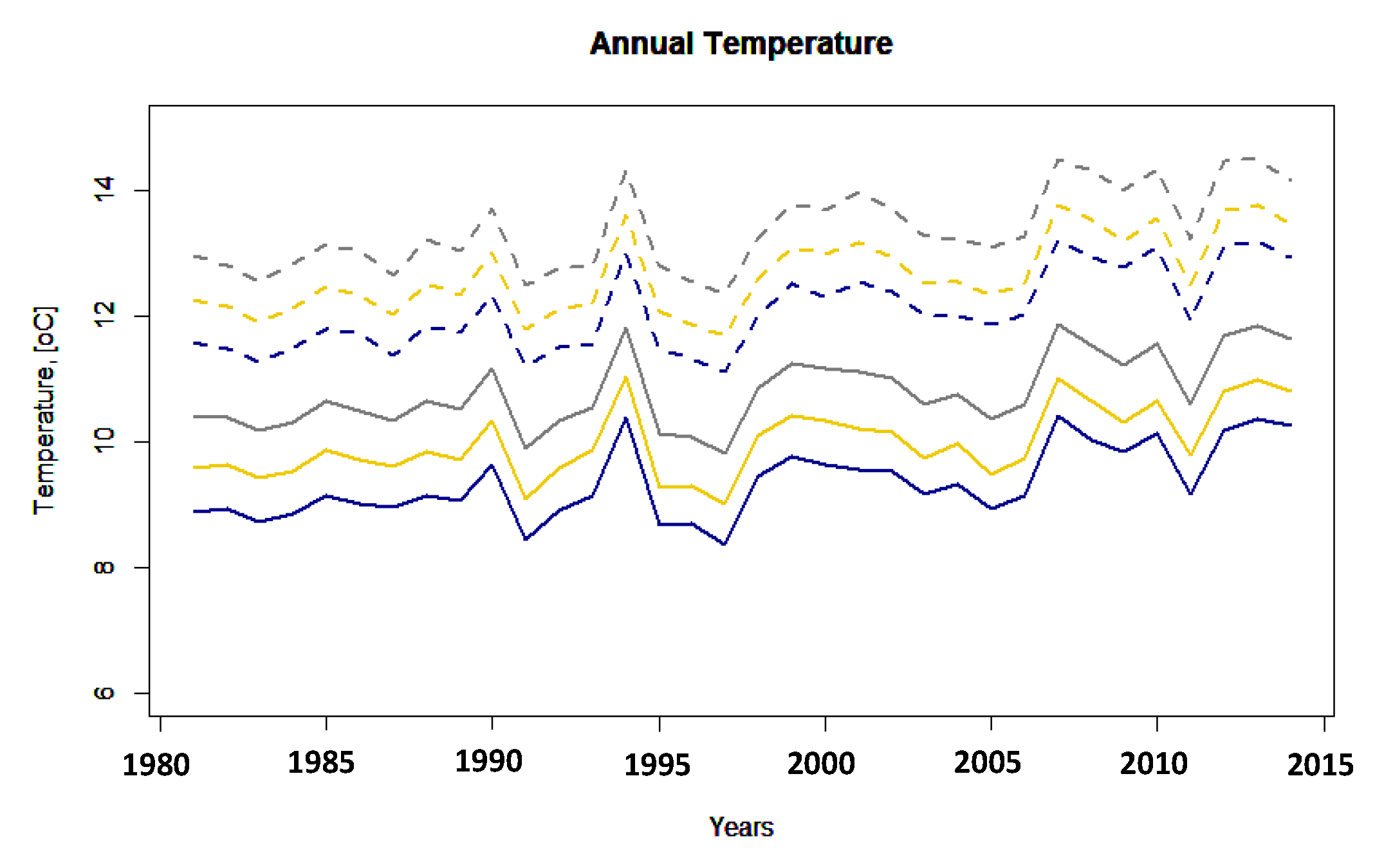
The annual temperature line plots for the northern (solid lines) and southern (dashed lines) Mesta/Nestos catchment are demonstrated in Figure 3. The different colors attribute the results of ERAI_50 (gray-colored curves), ERAI_25 (yellow-colored curves), and ERAI_12.5 (blue-colored curves) spatial analysis. As shown in the figure, there was a difference of almost 2.0–3.0 °C between the temperature of the northern and the southern parts of the basin, since the northern part is dominated by high mountains while the southern part gets gradually flatter upon approaching to the sea. The temperature difference was detected for all the evaluated data resolutions. Additionally, the data with the highest resolution (0.125° × 0.125°) presented the lowest temperature in both areas, while the data of 0.50° × 0.50° resolution were associated with the highest temperatures. The temperature for ERAI_25 varied between the temperatures of high- and low-resolution datasets.
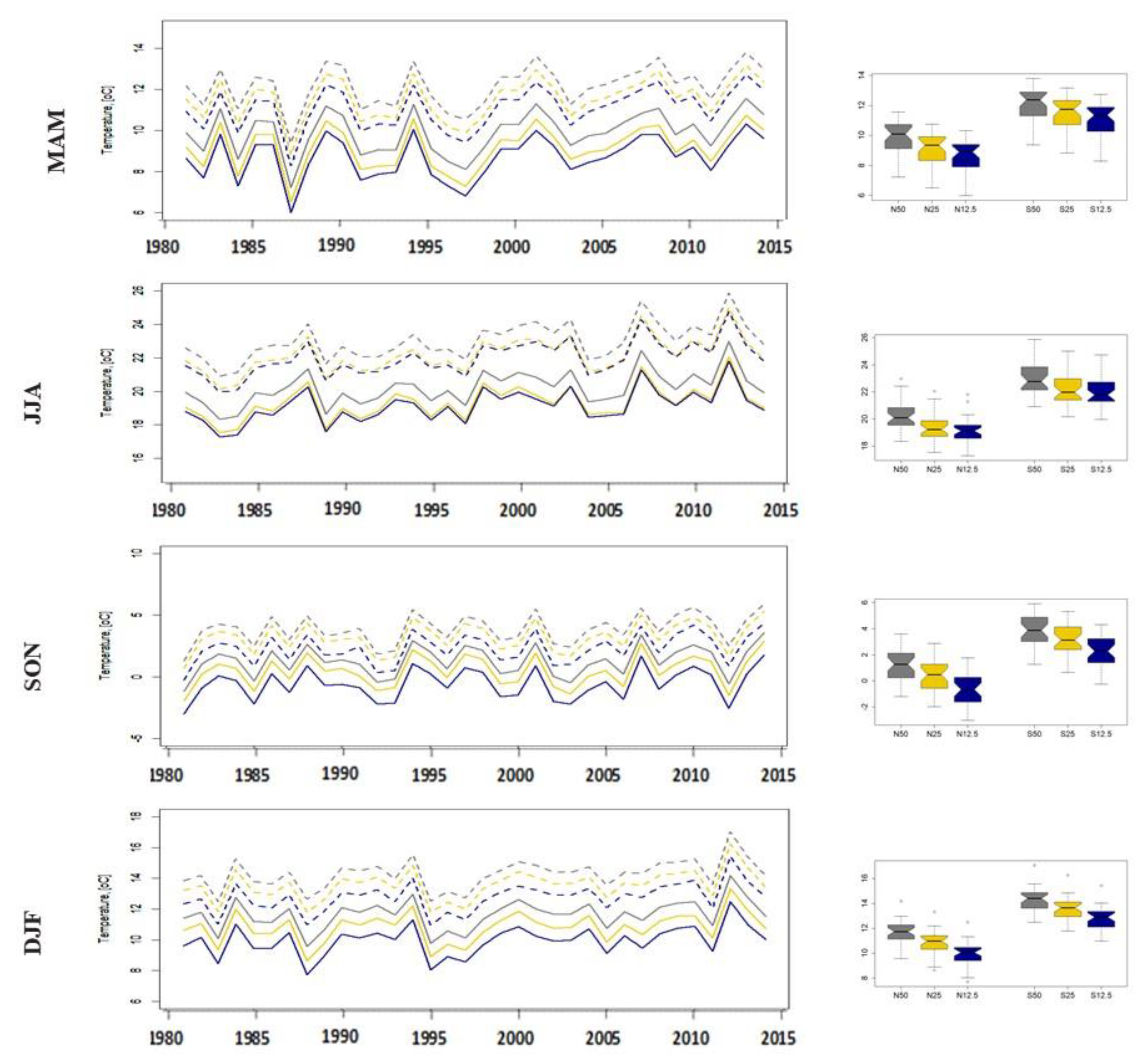
The seasonal diagram, as depicted in Figure 4, shows that the southern part of the basin had the highest temperatures during the whole year (all seasons). Additionally, the temperatures (blue colored lines) derived from the higher-resolution spatial analysis datasets were the lowest in both areas and during all seasons, while those derived from the coarser-resolution datasets were the highest (gray-colored lines). The most evident temperature bias between the two regions was detected during summer, with the southern flat region warmer than the northern mountainous region by about 2.0–3.0 °C. According to the seasonal graphs, the second warmest season was spring (MAM: March–April–May). The corresponding boxplots describe the difference between the northern and the southern parts of the Mesta/Nestos basin for the three spatial resolutions (N50–S50: gray; N25–S25: yellow; N12.5–S12.5: blue).
3.2. Climate Analysis of Precipitation Data
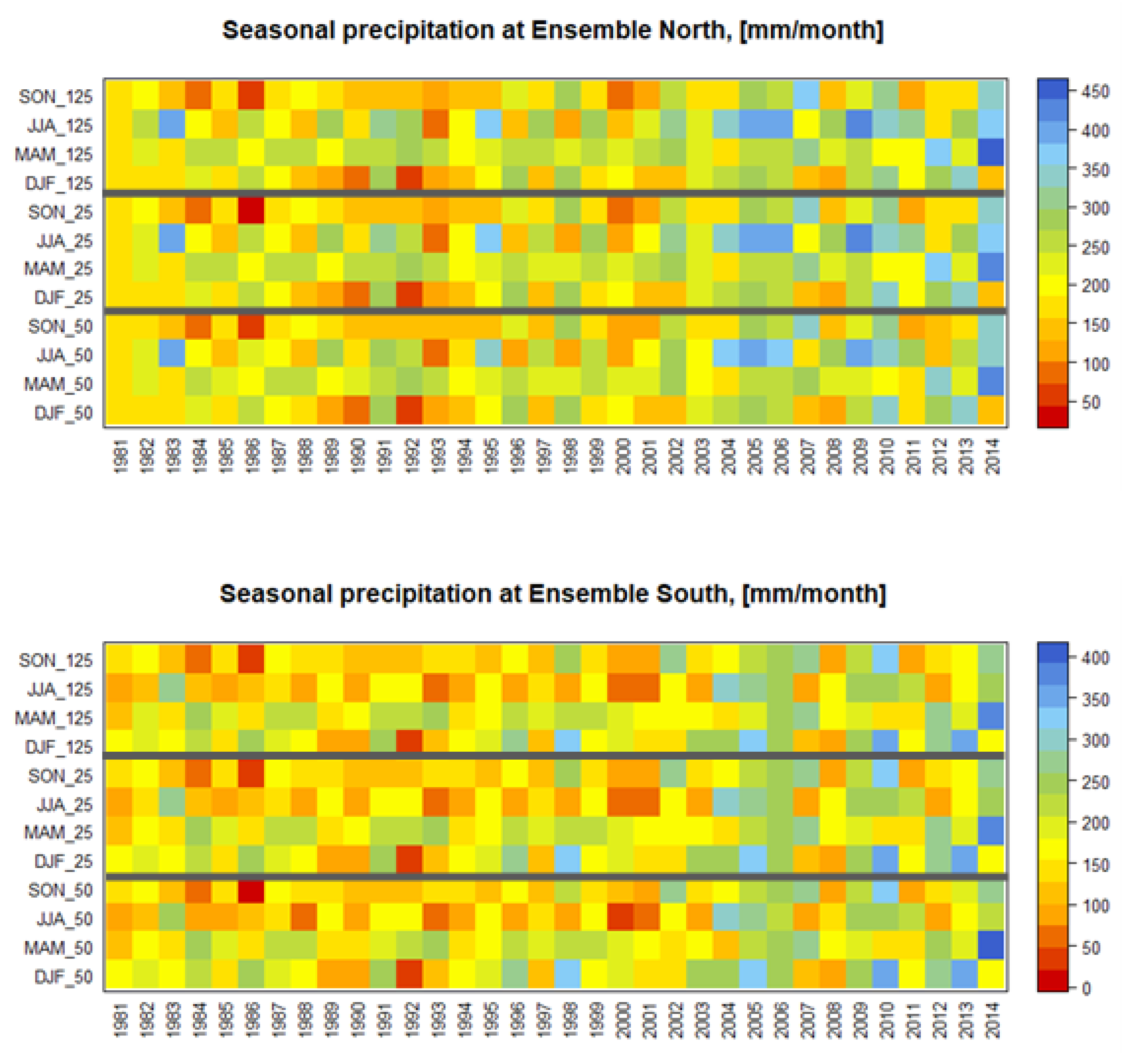
The results for the precipitation parameter show that the southern part of the basin, which is the warmest, was also the driest, since its precipitation was almost 100 mm lower than that of the upstream part. The most important output for the precipitation variable was that all the datasets with different spatial resolution presented almost equal results. The statistics of the annual results can be seen in Table 1, where the values of the mean, maximum, interquartile range (IQR), standard deviation (SD), skewness, and kurtosis are presented for the two parts of the basin and for all resolutions. According to the analysis, the mean, maximum, and IQR values were higher in the northern part of the basin, e.g., the mean precipitation of N50 and S50 (N50 and S50 stands for the northern and southern parts of basin with data at 0.50° × 0.50°, respectively) was equal to 2.3 mm and 1.9 mm, respectively. The skewness and kurtosis were lower in the northern than in the southern part, while the standard deviation was almost equal in both parts of the basin. The results between the different spatial analyses in the same area presented no differences. As it can be seen in Table 1, in both areas, the climatic characteristics of precipitation were very close, meaning that the lowest-resolution spatial analysis could provide the same accuracy as the highest one.
The corresponding seasonal results for the two basin regions and for the three spatial resolutions are demonstrated in Figure 5. In both parts of the basin, the three spatial analyses had almost equal results during the four seasons and during the 35 years of data availability. The results were equal in most years except for some very specific cases. For example, in 1982, in both areas, the analysis of the ERA_12.5 data presented slightly higher precipitation for the summer season (JJA: June–July–August), while, in the year 2000, the data derived from the lowest-resolution dataset presented a slightly lower precipitation during summer (north part of the basin) and slightly more rainfall during autumn (southern part of the basin). It should be mentioned that, after 2003, the wet seasons were more obvious in both parts of the basin, while the previous years were characterized by drought conditions, particularly the years of 1984, 1986, and 1992 for both parts of the basin, while the years 2000 and 2001 were more intense in the southern part of the basin.
3.3. Hydrologic Model Outputs
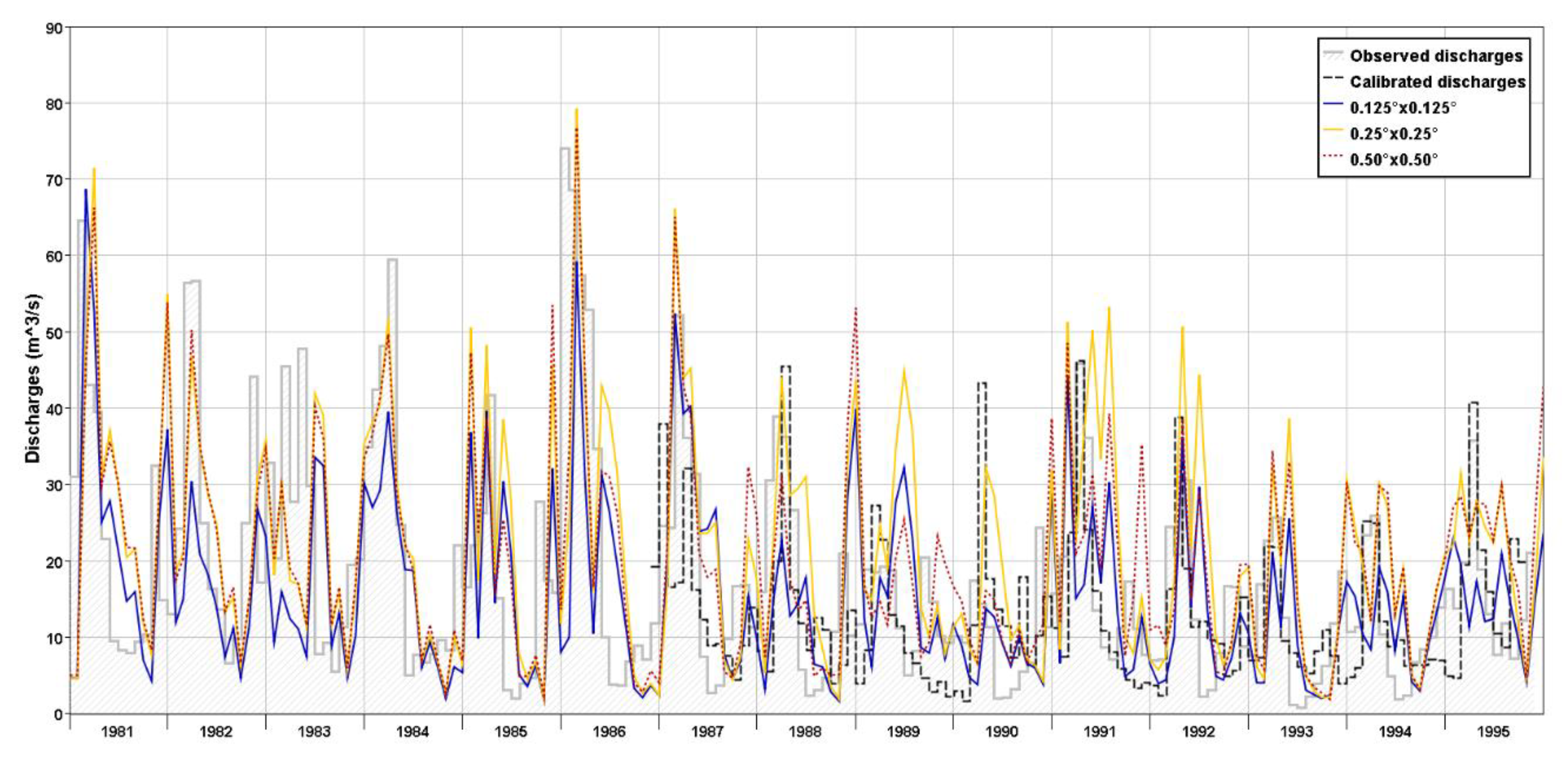
Altogether, the simulation results demonstrated a satisfactory correlation among the observed discharges and the simulated ones, as depicted in Figure 6. In terms of streamflow seasonality, the simulated discharges followed the Mediterranean area’s pattern, i.e., high flows during late winter and spring, and low flows during summer and autumn. In the case of ERAI_50 and ERAI_25, the average discharges over the designated period from 1981 to 1995 were 20.7 m3/s and 21.9 m3/s, respectively. The aforementioned discharges were relatively higher than the 18.1 m3/s that was observed during the same period. This means that, in the case of ERAI_50 and ERAI_25, there was an overestimation of the river discharges of approximately 14.3% and 20.9%, respectively. On the other hand, for the ERAI_12.5 simulation, the discharges were equal to 15.8 m3/s, i.e., there is an underestimation of approximately 13.7% of the runoff. Moreover, in all simulation runs, the observed dry period of 1989 to 1994 was clearly depicted, as well as the maximum monthly flows that occurred in the period 1986–1987.
Regarding the observed discharges at the interannual (15 years of data) time scale, the maxima of 34.8 m3/s and 35.7 m3/s occurred during April and May, as demonstrated in Figure 7 for the MAM (March–April–May) time period. The simulated discharges of 31.1 m3/s at 0.50° × 0.50°, 33.7 m3/s at 0.25° × 0.25°, and 23.9 m3/s at 0.125° × 0.125° resolution are shown for the same period. As for the minimum discharges, all scenarios matched the observed minimum flows in autumn. The observed minimum of 5.5 m3/s in September was slightly lower than the 7.7 m3/s and 6.5 m3/s of the ERAI_50 and ERAI_25, as demonstrated in Figure 7 for the SON (September–October–November) time period. For the ERAI_12.5 simulations, the minimum of 5.6 m3/s occurred in October. The relatively high streamflows of June, as shown in the JJA (June–July–August) diagram of Figure 7, were attributed to increased precipitation that generally occurs during the beginning of the summer season.
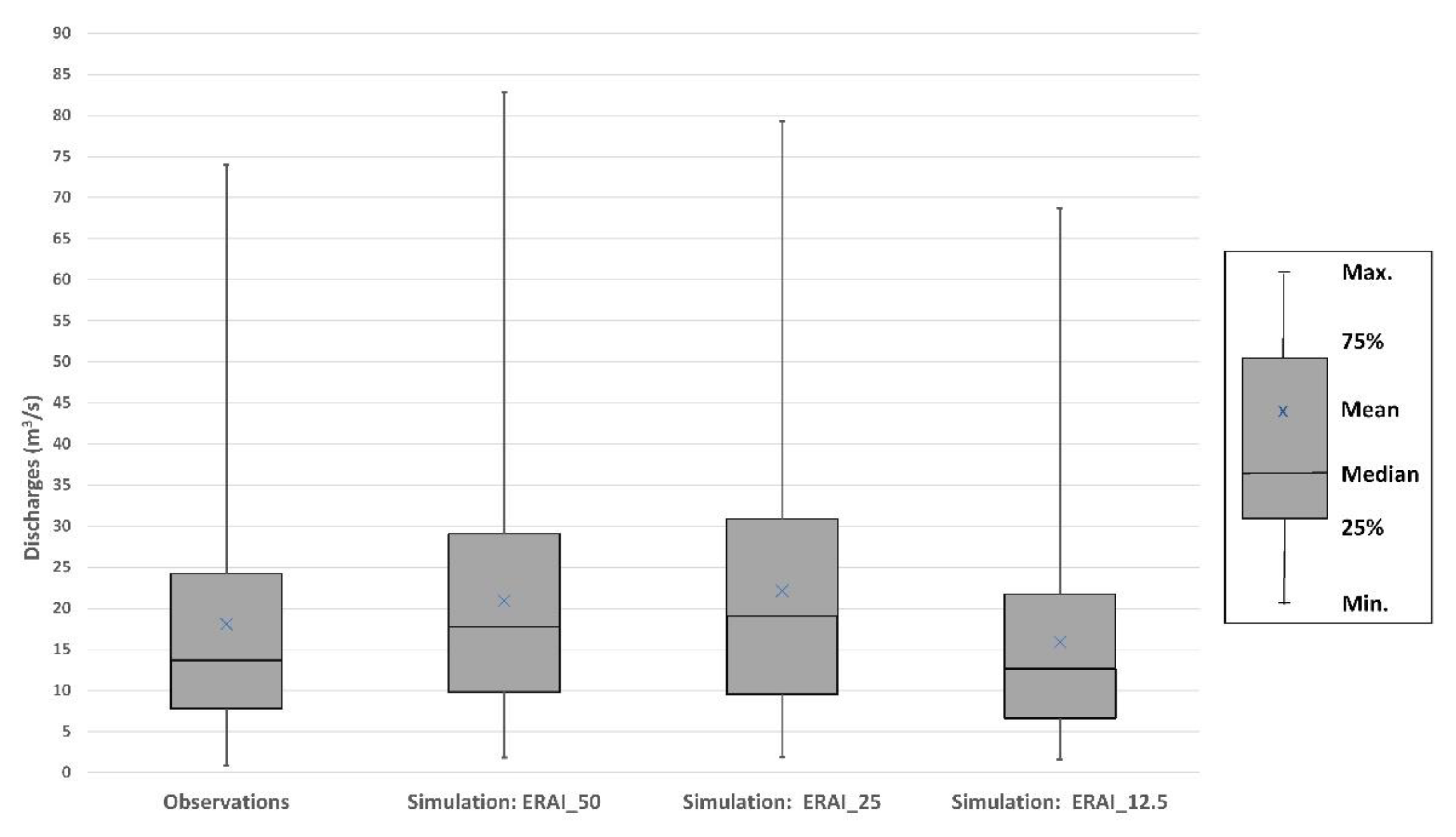
The coefficient of determination R2 for the simulations was equal to 0.63 for the 0.125° × 0.125°, 0.69 for the 0.25° × 0.25°, and 0.66 for the 0.50° × 0.50° simulation. At the same time, the PBIAS for the same sequence of simulations was 24.81, −8.82, and −3.31, respectively. The monthly analysis of the results (Figure 8) revealed an increased correlation of all the datasets. In particular, the observed minimum flow of 0.9 m3/s was of the same magnitude as the 1.8 m3/s (ERAI_50), 1.9 m3/s (ERAI_25), and 1.6 m3/s (ERAI_12.5) simulations. At the same time, the maximum discharge of 74.0 m3/s was comparable to 82.8 m3/s (ERAI_50), 79.3 m3/s (ERAI_25), and 68.7 m3/s (ERAI_12.5). The median of all the datasets ranged between 12.5 m3/s and 19.0 m3/s, with the minimum and maximum values related to 0.125° × 0.125° and 0.25° × 0.25° simulations, respectively. Finally, what can also be observed is that the interquartile range, i.e., the area between the upper and lower quartiles, of the ERAI_50 and ERAI_25 datasets was almost identical.
4. Discussion
The aim of the present research was to assess the spatial resolution of reanalysis climatic data below or over which the hydrologic modeling simulation was not affected by the scale of the inputs. To address this issue, three different reanalysis datasets of 0.50° × 0.50°, 0.25° × 0.25°, and 0.125° × 0.125° resolution were used as inputs to a spatially distributed hydrologic model in order to generate discharges of a study basin.
The literature demonstrates a number of researches where either reanalysis products were evaluated with ground truth data [23,25,26] or reanalysis products of different origin were used for hydrologic simulations. Regarding the latter, Essou et al. [22] investigated the hydrologic response of 370 watersheds based on three reanalysis products with the same spatial resolution. The watershed areas ranged between 104 and 10,325 km2, and they were allocated in five different climatic regions, including the Mediterranean and continental climates, which is the climate of the region to which the Mesta/Nestos basin belongs. The novelty of the current research consists of the assessment of reanalysis data coming from the same source, i.e., the ECMWF reanalysis product, but with different spatial resolutions, determining the performance of hydrologic simulations at a river basin scale. To the authors’ knowledge, no similar analysis regarding the impact of the spatial analysis of ERA reanalysis gridded data on the hydrologic modeling procedure is referenced in the literature. At the same time, apart from the sensitivity analysis of the simulated discharges for the ERAI_50, ERAI_25, and ERAI_12.5 datasets, the current research explicitly provides a comparative analysis of the aforementioned reanalysis gridded variables of precipitation and temperature, and important outputs are designated.
As for the gridded variables of temperature and precipitation, the performed analysis demonstrated that, in the case of temperatures, the lower temperatures originated from the data with the finer spatial resolution. On the other hand, the higher temperatures over the basin area were attributed to the data with coarser spatial analysis. This difference was observed as the higher-resolution datasets managed to detect the altitude and the vertical temperature gradient in a more detailed way. The representation of the terrain’s elevation in the case of finer-resolution datasets attributes the regional climatic characteristics in a more accurate manner, particularly in mountainous watersheds. In the case of a coarser mesh, these topographic variations are smoothed due to the average elevation that is attributed to each cell. Erum et al. [31] used three high-resolution gridded datasets with different resolutions, namely, NARR, ANUSPLIN, and CaPA, with resolutions of ~32 km, 10 km, and 15 km, respectively, for a case study area in western Canada. The coarsest of the three aforementioned datasets demonstrated warmer temperatures in all seasons except for winter, where the second in terms of resolution data presented almost the same outputs as the first. Regarding the precipitation variable, the analysis revealed negligible statistical differences in the two parts of the basin. The Mesta/Nestos catchment, due to its complex topography and adjacency to the north Aegean Sea, probably required much more than basic elevation information for the successful climate interpolation of precipitation data. This finding is consistent with that of Daly et al. [33] and Leung and Qian [50], who proved that elements such as elevation, location, the vicinity of the sea, catchment topographic orientation, and vertical atmospheric layer are essential for the interpolation of precipitation.
The catchment size seems to affect the impact of resolution of precipitation input on stream discharge, since the impact of fine-resolution precipitation input was negligible for the specific catchment. In small catchment areas up to 100.0 km2, Berne et al. [51] demonstrated that, under specific characteristics, such as a slope between 1% and 10%, impermeability between 10% and 60%, and the Mediterranean climate, the required resolution of precipitation input should be 5.2 km. For catchment areas larger than 1000 km2, it was demonstrated [52] that they are not highly affected by the spatial resolution of precipitation. According to Fu et al. [52], all simulations that are related to lower discharges are linked with datasets of finer resolution, apart from during the warm periods of the year. Temperature variability seems to be a primary factor of discharge reduction at the lower resolution, while rainfall coverage can remain a principal factor at finer resolutions. Kouwen [53] also showed in his research that lower-resolution radar rainfall data of 10.0 km × 10.0 km can sufficiently be used for modeling floods compared to higher-resolution data of 2.0 km × 2.0 km.
The increased resolution has the benefit of reducing numerical truncation errors [54], while it permits the simulation of fine-scale details. However, in complex terrains, such as mountainous areas coupled with plains, and in complex climates, such as continental climate effected by seacoast climate, lower-resolution data might be more suitable for the simulation and prediction of the temperature [55]. Colle et al. [56] reached similar conclusions by indicating that higher resolution is more sensitive to the convective parameterization and reduces the accuracy of climate parameters, especially when the topography is complex. As demonstrated in the results, in the case of low and medium resolution, the overestimation of the discharges was on the order of 14.3% and 20.9%, respectively, while, in the case of higher resolution, there was an underestimation of 13.7%. Similar hydrologic modeling performance was presented in a German catchment of approximately 4000 km2 [57]. That research, where the spatial variation was based on kriging from point measurements, proved that simulations with coarser-resolution data outperformed the finer-resolution simulations. On the other hand, Haddeland et al. [58] concluded that, when the topographic and land-cover data resolution is altered, as well as the forcing variables, then the coarser-resolution forced simulations are more biased than finer-resolution simulations. In any case, since the runoff response of a watershed is not directly proportional to precipitation, but it is also governed by the physical characteristics of a watershed (e.g., topography, soil, and land cover), differences in the timing and volume of the produced discharges is bound to occur. The need for amelioration of the distributed model structure to make better use of inputs of fine resolution could be proposed as a solution to the simulation process uncertainty. The later output agrees with Bell and Moore [59], who demonstrated in their research, contrary to what they initially believed, that, in the case of gridded rainfalls, the best performance is obtained when lower-resolution radar data are utilized, and they suggested a revision of the model structure.
An additional reason behind the simulated outputs is the dependence of the river’s flow, particularly in the summer period, on the snowmelt process. The temperature is the principal variable that affects the melting of snow when using a snowmelt runoff model. For the current case basin, the overestimated discharges of ERAI_50 and EAI_25 data coincided with the high temperatures that were presented in both datasets. Thus, it is believed that the ERA dataset resolution does not compensate for errors in the model calibration in the region. However, the application of different hydrological models that contain snowmelt-computing options could provide different outputs, since each model has its own snowmelt algorithm. Verden et al. [60] investigated the performance of snowmelt algorithms that are integrated into watershed models, namely, HEC-1, SSARR UBC, NWSRFS, PRMS, SHE, SRM, and TANK, and they reached the conclusion that different snowpack melt quantities were derived from each model in the same case area. Jain et al. [61] demonstrated that warmer climatic conditions increase the annual stream flow but not severely. At the same time, Lutz et al. [62] concluded that, in the case of climate change, i.e., increased temperatures, the snowmelt process is caused by an increase in precipitation and from accelerated melt due to the higher temperatures. The aforementioned finding might be contradictory to the temperature’s impact on evapotranspiration, meaning that high temperatures result in increased evapotranspiration and, hence, decreased water flows. However, Koedyk and Kingston [63], in order to investigate the influence of PET on a river’s runoff, used six different PET methods for a temperature increase of 2.0 °C as derived from five general circulation models. The output of their research demonstrated that, in rivers of continuous flow, the impact is relatively small, i.e., under 5% at the monthly scale and at most 5.2% at the annual scale.
Concerning the accuracy of the simulated discharges, their statistical assessment demonstrated the reliability of the outputs, i.e., R2 > 0.63 for each of the simulated datasets, since values greater than 0.5 are typically considered acceptable [64]. It should be mentioned that the derived model evaluation statistics are sensitive to high values (outliers) and insensitive to additive and proportional differences between model predictions and measured data [65]. However, the daily and monthly datasets used in this study do not fall into the previous categories. As for the PBIAS method, low-magnitude values indicate accurate model simulation, as in the case of the 0.50° × 0.50° and 0.25° × 0.25° resolution, while positive and negative values indicate model underestimation and overestimation bias, respectively [48]. Moreover, according to the general performance ratings for recommended statistics for a monthly time step [65], a PBIAS (%) of the streamflow with ranges of ±10 < PBIAS < ±15 and ±15 < PBIAS < ±25 is considered good and satisfactory, respectively. In the proposed research, the results derived from climate data of 0.50° × 0.50° and 0.25° × 0.25° (PBIAS equal to −3.31 and −8.82, respectively) were classified as good, and those of 0.125° × 0.125° (PBIAS equal to +24.2) were classified as satisfactory [66].
Considering the number of areas in Europe, as well as other parts of the world, where dense meteorological monitoring networks are lacking, the potential offered by the gridded and reanalysis datasets is unique. The proposed research outputs are considered appropriate for assisting the selection of reanalysis data resolution, mostly in cases with similar geomorphological characteristics and climatic conditions. Moreover, since the climatic change impact on water resources is ongoing research, it is believed that the present study could offer added value to the selection process of reanalysis data that will be used for the bias correction of climate change datasets.
5. Conclusions
Data availability and, in particular, precipitation and temperature data series are crucial for the hydrologic simulation of river basins. Apart from the accuracy and reliability of data, their spatial coverage and density have increased impact on the hydrologic modeling behavior. Currently, the availability of gridded dataset products of various resolutions provides solutions in areas of coarse gauge networks or even in regions with a lack of observations. However, this plethora of data sources that provide meteorological and climatological variables at meshes of varying resolution could be a bottleneck in hydrologic modeling.
The assessment of the impact of three different ERA-Interim reanalysis datasets, in terms of spatial resolution, on river basin hydrology suggests that, for the runoff simulations at a daily time step, the most appropriate dataset is of medium resolution. The produced biases in the case of climatic variables of coarser or more refined resolution are relatively low (≤ ±10%); thus, these data could also be used for the long-term management of water resources. An important factor of the outputs is the dependence of the summer runoff on the snowmelt process. Moreover, the scale of the basin plays an important role in the selection of the most appropriate resolution. Overall, the results presented that reanalysis data sources could be used as proxies to successfully force hydrological models. Finally, the proposed research could also shed light in studies focusing on climate change impacts on hydrology; thus, the question whether climate input data having higher spatial resolution result in better model simulations could be explored.
Author Contributions
In this research, all authors equally contributed to the conceptualization of the paper, the simulations, and the interpretation of the outputs, as well as to the writing, review, and editing of the paper. All authors have read and agreed to the published version of the manuscript.
Funding
This research received no external funding.
Conflicts of Interest
The authors declare no conflicts of interest.
References
- Brigode, P.; Oudin, L.; Perrin, C. Hydrological model parameter instability: A source of additional uncertainty in estimating the hydrological impacts of climate change? J. Hydrol. 2013, 476, 410–425. [Google Scholar] [CrossRef] [Green Version]
- Refsgaard, J.C.; Storm, B. Construction, Calibration and Validation of Hydrological Models. In Distributed Hydrological Modelling. Water Science and Technology Library; Abbott, M.B., Refsgaard, J.C., Eds.; Springer: Dordrecht, Netherlands, 1990; Volume 22. [Google Scholar]
- O’Riordan, T. Environmental Science for Environmental Management; Routledge: London, UK, 2014. [Google Scholar]
- Chen, Y.C.; Wei, C.; Yeh, H.C. Rainfall network design using kriging and entropy. Hydrol. Process. 2008, 22, 340–346. [Google Scholar] [CrossRef]
- Xu, H.; Xu, C.Y.; Chen, H.; Zhang, Z.; Li, L. Assessing the influence of rain gauge density and distribution on hydrological model performance in a humid region of China. J. Hydrol. 2013, 505, 1–12. [Google Scholar] [CrossRef]
- Anctil, F.; Lauzon, N.; Andréassian, V.; Oudin, L.; Perrin, C. Improvement of rainfall–runoff forecasts through mean areal rainfall optimization. J. Hydrol. 2006, 328, 717–725. [Google Scholar] [CrossRef]
- Woods, R.A.; Sivapalan, M.; Duncan, M. Investigating the representative elementary area concept: An approach based on field data. Hydrol. Process. 1995, 6, 291–312. [Google Scholar] [CrossRef]
- Bathurst, J.C. Physically based distributed modeling of upland catchment using the Systeme Hydrologique Europeen. J. Hydrol. 1986, 87, 79–123. [Google Scholar] [CrossRef]
- World Meteorological Organization. Density of stations for a network. In Hydrology—From Measurement to Hydrological Information, Vol 1, Guide to Hydrological Practices, 6th ed.; WMO-168; World Meteorological Organization: Geneva, Switzerland, 2008. [Google Scholar]
- Khan, A.J.; Koch, M.; Chinchilla, K.M. Evaluation of Gridded MultiSatellite Precipitation Estimation (TRMM-3B42-V7) Performance in the Upper Indus Basin (UIB). Climate 2018, 6, 76. [Google Scholar] [CrossRef] [Green Version]
- Rossi, M.; Kirschbaum, D.; Valigi, D.; Mondini, A.; Guzzetti, F. Comparison of Satellite Rainfall Estimates and Rain Gauge Measurements in Italy, and Impact on Landslide Modeling. Climate 2017, 5, 90. [Google Scholar] [CrossRef] [Green Version]
- Haylock, M.R.; Hofstra, N.; Klein Tank, A.M.G.; Klok, E.J.; Jones, P.D.; New, M. A European daily high-resolution gridded data set of surface temperature and precipitation for 1950–2006. J. Geophys. Res. 2008, 113. [Google Scholar] [CrossRef] [Green Version]
- Lazoglou, G.; Anagnostopoulou, C.; Skoulikaris, C.; Tolika, K. Bias Correction of Climate Model’s Precipitation Using the Copula Method and Its Application in River Basin Simulation. Water 2019, 11, 600. [Google Scholar] [CrossRef] [Green Version]
- Nerini, D.; Zulkafli, Z.; Wang, L.; Onof, C.; Buytaert, W.; Lavado-Casimiro, W.; Guyot, J. A Comparative Analysis of TRMM–Rain Gauge Data Merging Techniques at the Daily Time Scale for Distributed Rainfall–Runoff Modeling Applications. J. Hydrometeorol. 2015, 16, 2153–2168. [Google Scholar] [CrossRef] [Green Version]
- Nastos, P.T.; Kapsomenakis, J.; Douvis, K.C. Analysis of precipitation extremes based on satellite and high-resolution gridded data set over Mediterranean basin. Atmos. Res. 2013, 131, 46–59. [Google Scholar] [CrossRef]
- Adam, J.C.; Lettenmaier, D.P. Adjustment of global gridded precipitation for systematic bias. J. Geophys. Res. Atmos. 2003, 108, 4257. [Google Scholar] [CrossRef]
- Faiz, M.A.; Liu, D.; Fu, Q.; Sun, Q.; Li, M.; Baig, F.; Li, T.; Cui, S. How accurate are the performances of gridded precipitation data products over Northeast China? Atmos. Res. 2018, 211, 12–20. [Google Scholar] [CrossRef]
- Hofstra, N.; Haylock, M.; New, M.; Jones, P.D. Testing E-OBS European high-resolution gridded data set of daily precipitation and surface temperature. J. Geophys. Res. 2009, 114. [Google Scholar] [CrossRef]
- Gao, L.; Schulz, K.; Bernhardt, M. Statistical downscaling of ERA-interim forecast precipitation data in complex terrain using lasso algorithm. Adv. Meteorol. 2014, 2014. [Google Scholar] [CrossRef] [Green Version]
- Jahani, B.; Mohammadi, B. A comparison between the application of empirical and ANN methods for estimation of daily global solar radiation in Iran. Theor. Appl. Climatol. 2019, 137, 1257. [Google Scholar] [CrossRef]
- Fuka, D.R.; Walter, M.T.; MacAlister, C.; Degaetano, A.T.; Steenhuis, T.S.; Easton, Z.M. Using the Climate Forecast System Reanalysis as weather input data for watershed models. Hydrol. Process. 2014, 28, 5613–5623. [Google Scholar]
- Essou, G.R.C.; Sabarly, F.; Lucas-Picher, P.; Brissette, F.; Poulin, A. Can precipitation and temperature from meteorological reanalyses be used for hydrological modeling? J. Hydrometeorol. 2016. [Google Scholar] [CrossRef]
- Dee, D.; Uppala, S.M.; Simmons, A.J.; Berrisford, P.; Poli, P.; Kobayashi, S.; Andrae, U.; Balmaseda, M.A.; Balsamo, G.; Bauer, P.; et al. The ERA-Interim reanalysis: Configuration and performance of the data assimilation system. Quart. J. R. Meteor. Soc. 2011, 137, 553–597. [Google Scholar] [CrossRef]
- Bosilovich, M.G. Regional climate and variability of NASAMERRA and recent reanalyses: U.S. summertime precipitation and temperature. J. Appl. Meteor. Climatol. 2013, 52, 1939–1951. [Google Scholar] [CrossRef]
- Lorenz, C.; Kunstmann, H. The hydrological cycle in three state-of-the-art reanalyses: Intercomparison and performance analysis. J. Hydrometeorol. 2012, 13, 1397–1420. [Google Scholar] [CrossRef] [Green Version]
- Grusson, Y.; Anctil, F.; Sauvage, S.; Sánchez Pérez, J.M. Testing the SWAT Model with Gridded Weather Data of Different Spatial Resolutions. Water 2017, 9, 54. [Google Scholar] [CrossRef] [Green Version]
- Gao, L.; Bernhardt, M.; Schulz, K. Elevation correction of ERA-Interim temperature data in complex terrain. Hydrol. Earth Syst. Sci. 2012, 16, 4661–4673. [Google Scholar] [CrossRef] [Green Version]
- Muppa, S.K.; Anandan, V.K.; Kesarkar, K.A.; Rao, S.V.B.; Reddy, P.N. Study on deep inland penetration of sea breeze over complex terrain in the tropics. Atmospheric. Res. 2012, 104, 209–216. [Google Scholar] [CrossRef]
- Hu, Z.; Hu, Q.; Zhang, C.; Chen, X.; Li, Q. Evaluation of reanalysis, spatially interpolated and satellite remotely sensed precipitation data sets in central Asia. J. Geophys. Res. Atmos. 2016, 121, 5648–5663. [Google Scholar] [CrossRef] [Green Version]
- Donat, M.G.; Sillmann, J.; Wild, S.; Alexander, L.V.; Lippmann, T.; Zwiers, F.W. Consistency of Temperature and Precipitation Extremes across Various Global Gridded In Situ and Reanalysis Datasets. J. Clim. 2014, 27, 5019–5035. [Google Scholar] [CrossRef]
- Eum, H.I.; Dibike, Y.; Prowse, T.; Bonsal, B. Inter-comparison of high-resolution gridded climate data sets and their implication on hydrological model simulation over the Athabasca Watershed, Canada. Hydrol. Process. 2014, 28, 4250–4271. [Google Scholar] [CrossRef]
- Lundquist, J.D.; Minder, J.R.; Neiman, P.J.; Sukovich, E. Relationships between Barrier Jet Heights, Orographic Precipitation Gradients, and Streamflow in the Northern Sierra Nevada. J. Hydrometeorol. 2010, 11, 1141–1156. [Google Scholar] [CrossRef] [Green Version]
- Daly, C.; Halbleib, M.; Smith, J.I.; Gibson, W.P.; Doggett, M.K.; Taylor, G.H.; Curtis, J.; Pasteris, P.P. Physiographically sensitive mapping of climatological temperature and precipitation across the conterminous United States. Int. J. Climatol. A J. R. Meteorol. Soc. 2011, 28, 2031–2064. [Google Scholar] [CrossRef]
- Woo, M.K.; Thorne, R. Snowmelt contribution to discharge from a large mountainous catchment in subarctic Canada. Hydrol. Process. 2006, 20, 2129–2139. [Google Scholar] [CrossRef]
- Bhattacharya, T.; Khare, D.; Arora, M. A case study for the assessment of the suitability of gridded reanalysis weather data for hydrological simulation in Beas river basin of North Western Himalaya. Appl. Water Sci. 2019, 9, 110. [Google Scholar] [CrossRef] [Green Version]
- Tarek, M.; Brissette, F.P.; Arsenault, R. Evaluation of the ERA5 reanalysis as a potential reference dataset for hydrological modeling over North-America. Hydrol. Earth Syst. Sci. Discuss. 2019. [Google Scholar] [CrossRef]
- Skoulikaris, C.H.; Ganoulis, J. Climate Change Impacts on River Catchment Hydrology Using Dynamic Downscaling of Global Climate Models. In National Security and Human Health Implications of Climate Change, NATO Science for Peace and Security Series C: Environmental Security; Fernando, H., Klaić, Z., McCulley, J., Eds.; Springer: Berlin, Germany, 2012; pp. 281–287. [Google Scholar]
- Bank of Greece. Environmental, Economic and Social Impacts Due to Climate Change in Greece; Bank of Greece: Athens, Greece, 2011; p. 546. [Google Scholar]
- UNECE. Second Assessment of Transboundary Rivers, Lakes and Groundwaters; UNECE: Geneva, Switzerland, 2011. [Google Scholar]
- Balsamo, G.; Albergel, C.; Beljaars, A.; Boussetta, S.; Brun, E.; Cloke, H.; De Rosnay, P. ERA-Interim/Land: A global land surface reanalysis data set. Hydrol. Earth Syst. Sci. 2015, 19, 389–407. [Google Scholar] [CrossRef] [Green Version]
- Ledoux, E.; Girard, G.; de Marsily, G.; Deschenes, J. Spatially distributed modelling: Conceptual approach, coupling surface water and ground water. In Unsaturated Flow Hydrologic Modelling-Theory and Practice; Morel-Seytoux, H.J., Ed.; NATO ASI Series S 275; Kluwer Academic: Boston, CA, USA, 1989; pp. 435–454. [Google Scholar]
- Violette, S.; Ledoux, E.; Goblet, P.; Carbonnel, J.-P. Hydrologic and thermal modeling of an active volcano: The Piton de la Fournaise, Reunion. J. Hydrol. 1997, 191, 37–63. [Google Scholar] [CrossRef]
- Artinyan, E.; Habets, F.; Noilhan, J.; Ledoux, E.; Dimitrov, D.; Martin, E.; Le Moigne, P. Modelling the water budget and the riverflows of the Maritsa basin in Bulgaria. Hydrol. Earth Syst. Sci. 2008, 12, 21–37. [Google Scholar] [CrossRef] [Green Version]
- Natural Resources Conservation Service (NRCS). National Engineering Handbook, Part 630 Hydrology; U.S. Department of Agriculture: Washington, DC, UAS, 1993; Chapt. 11, Snowmelt.
- Rango, A.; Martinec, J. Revisiting the degree-day method for snowmelt computations. J. Am. Water Resour. Assoc. 1995, 31, 657–669. [Google Scholar] [CrossRef]
- Etchevers, P.; Golaz, C.; Habets, F. Simulation of the water budget and the river flows of the Rhone basin from 1981 to 1994. J. Hydrol. 2001, 244, 60–85. [Google Scholar] [CrossRef]
- Etchevers, P.; Martin, E. Impact d’un changement climatique sur le manteau neigeux et l’hydrologie des bassins versants de montagne. In Proceedings of the Colloque International «L’eau en montagne», Mégève, France, 6 September 2002. [Google Scholar]
- Gupta, H.V.; Sorooshian, S.; Yapo, P.O. Status of automatic calibration for hydrologic models: Comparison with multilevel expert calibration. J. Hydrologic. Eng. 1999, 4, 135–143. [Google Scholar] [CrossRef]
- Jolliffe, I.T.; Cadima, J. Principal component analysis: A review and recent developments. Phil. Trans. R. Soc. A 2016, 374, 20150202. [Google Scholar] [CrossRef]
- Leung, L.R.; Qian, Y. The sensitivity of precipitation and snowpack simulations to model resolution via nesting in regions of complex terrain. J. Hydrometeorol. 2003, 4, 1025–1043. [Google Scholar] [CrossRef]
- Berne, A.; Delrieu, G.; Creutin, J.D.; Obled, C. Temporal and spatial resolution of rainfall measurements required for urban hydrology. J Hydrol. 2004, 299, 166–179. [Google Scholar] [CrossRef]
- Fu, S.; Sonnenborg, T.O.; Jensen, K.H.; He, X. Impact of Precipitation Spatial Resolution on the Hydrological Response of an Integrated Distributed Water Resources Model. Vadose Zone J. 2011, 10, 25–36. [Google Scholar] [CrossRef]
- Kouwen, N. SIMPLE—A Watershed Model for Flood Forecasting. Users’ Manual; Department of Civil Engineering, University of Waterloo: Waterloo, ON, Canada, 1986; p. 130. [Google Scholar]
- Wang, X.; Steinle, P.; Seed, A.; Xiao, Y. The Sensitivity of Heavy Precipitation to Horizontal Resolution, Domain Size, and Rain Rate Assimilation: Case Studies with a Convection-Permitting Model. Adv. Meteorol. 2016, 2016. [Google Scholar] [CrossRef]
- Giunta, G.; Salerno, R.; Ceppi, A.; Ercolani, G.; Mancini, M. Effects of Model Horizontal Grid Resolution on Short- and Medium-Term Daily Temperature Forecasts for Energy Consumption Application in European Cities. Adv. Meteorol. 2019, 2019. [Google Scholar] [CrossRef]
- Colle, B.A.; Olson, J.B.; Tongue, J.S. Multiseason verification of the MM5. Part II: Evaluation of high-resolution precipitation forecasts over the northeastern United States. Weather. Forecast. 2003, 18, 458–480. [Google Scholar] [CrossRef]
- Das, T.; Bárdossy, A.; Zehe, E.; He, Y. Comparison of conceptual model performance using different representations of spatial variability. J. Hydrol. 2008, 356, 106–118. [Google Scholar] [CrossRef]
- Haddeland, I.; Matheussen, B.V.; Lettenmaier, D.P. Influence of spatial resolution on simulated streamflow in a macroscale hydrologic model. Water Resour. Res. 2002, 38, 291–2910. [Google Scholar] [CrossRef]
- Bell, V.A.; Moore, R.J. The sensitivity of catchment runoff models to rainfall data at different spatial scales. Hydrol. Earth Syst. Sci. 2000, 4, 653–667. [Google Scholar] [CrossRef]
- Verdhen, A.; Chahar, B.R.; Sharma, O.P. Snowmelt modelling approaches in watershed models: Computation and comparison of efficiencies under varying climatic conditions. Water Resour. Manag. 2014, 28, 3439–3453. [Google Scholar] [CrossRef]
- Jain, S.K.; Goswami, A.; Saraf, A.K. Assessment of Snowmelt Runoff Using Remote Sensing and Effect of Climate Change on Runoff. Water Resour. Manag. 2010, 24, 1763. [Google Scholar] [CrossRef]
- Lutz, A.F.; Immerzeel, W.W.; Shrestha, A.B.; Bierkens, M.F.P. Consistent increase in High Asia’s runoff due to increasing glacier melt and precipitation. Nat. Clim. Chang. 2014, 4, 587–592. [Google Scholar] [CrossRef] [Green Version]
- Koedyk, L.P.; Kingston, D.G. Potential evapotranspiration method influence on climate change impacts on river flow: A mid-latitude case study. Hydrol. Res. 2016, 47, 951–963. [Google Scholar] [CrossRef] [Green Version]
- Santhi, C.; Arnold, J.G.; Williams, J.R.; Dugas, W.A.; Srinivasan, R.; Hauck, L.M. Validation of the SWAT model on a large river basin with point and nonpoint sources. J. Am. Water Resour. Assoc. 2001, 37, 1169–1188. [Google Scholar] [CrossRef]
- Legates, D.R.; McCabe, G.J. Evaluating the use of “goodness-of-fit” measures in hydrologic and hydroclimatic model validation. Water Resour. Res. 1999, 35, 233–241. [Google Scholar] [CrossRef]
- Moriasi, D.N.; Arnold, J.G.; Van Liew, M.W.; Bingner, R.L.; Harmel, R.D.; Veith, T.L. Model evaluation guidelines for systematic quantification of accuracy in watershed simulations. Trans. ASABE 2007, 50, 885–900. [Google Scholar] [CrossRef]
Figure 1.
Case study basin with overlaying grids of the hydrologic model (gray rectangles) and of the 0.50° × 0.50° (blue cells), 0.25° × 0.25° (red cells), and 0.125° × 0.125° (green cells) ERA-Interim meshes.
Figure 1.
Case study basin with overlaying grids of the hydrologic model (gray rectangles) and of the 0.50° × 0.50° (blue cells), 0.25° × 0.25° (red cells), and 0.125° × 0.125° (green cells) ERA-Interim meshes.

Figure 2.
Representation of the MODSUR (modélisation de transfers de surface) hydrologic model operation mode.
Figure 2.
Representation of the MODSUR (modélisation de transfers de surface) hydrologic model operation mode.

Figure 3.
Line plot of annual temperature data for the northern (solid lines) and southern (dashed lines) parts of the Mesta/Nestos basin. Temperatures at 0.50° × 0.50°, 0.25° × 0.25°, and 0.125° × 0.125° resolution are represented in gray, yellow, and blue, respectively.
Figure 3.
Line plot of annual temperature data for the northern (solid lines) and southern (dashed lines) parts of the Mesta/Nestos basin. Temperatures at 0.50° × 0.50°, 0.25° × 0.25°, and 0.125° × 0.125° resolution are represented in gray, yellow, and blue, respectively.

Figure 4.
Line plots and boxplots of seasonal temperature data for the northern (solid line) and southern (dash line) parts of the basin. The temperatures at 0.50° × 0.50°, 0.25° × 0.25°, and 0.125° × 0.125° resolution are represented in gray, yellow, and blue, respectively.
Figure 4.
Line plots and boxplots of seasonal temperature data for the northern (solid line) and southern (dash line) parts of the basin. The temperatures at 0.50° × 0.50°, 0.25° × 0.25°, and 0.125° × 0.125° resolution are represented in gray, yellow, and blue, respectively.

Figure 5.
Seasonal precipitation data for north and south Mesta/Nestos catchment.

Figure 6.
Observed (hashed area) and initial calibrated (black dotted curve) discharges versus simulated discharges of 0.125° × 0.125°, 0.25° × 0.25°, and 0.50° × 0.50° spatial analysis (blue, yellow, and brown curves, respectively).
Figure 6.
Observed (hashed area) and initial calibrated (black dotted curve) discharges versus simulated discharges of 0.125° × 0.125°, 0.25° × 0.25°, and 0.50° × 0.50° spatial analysis (blue, yellow, and brown curves, respectively).

Figure 7.
Quarterly correlation of observed and simulated discharges at the political borders of the transboundary Mesta/Nestos river basin.
Figure 7.
Quarterly correlation of observed and simulated discharges at the political borders of the transboundary Mesta/Nestos river basin.

Figure 8.
Boxplots comparing the Mesta/Nestos river discharges, as derived from the hydrologic simulation of the basin under different input gridded datasets.
Figure 8.
Boxplots comparing the Mesta/Nestos river discharges, as derived from the hydrologic simulation of the basin under different input gridded datasets.


Table 1.
Statistics of the precipitation data at 50.0 × 50.0, 25.0 × 25.0, and 12.5 × 12.5 km resolution for the northern and southern parts of the Mesta/Nestos basin. IQR—interquartile range.
Table 1.
Statistics of the precipitation data at 50.0 × 50.0, 25.0 × 25.0, and 12.5 × 12.5 km resolution for the northern and southern parts of the Mesta/Nestos basin. IQR—interquartile range.
| N50 | N25 | N12.5 | S50 | S25 | S12.5 | |
|---|---|---|---|---|---|---|
| Mean | 2.3 | 2.4 | 2.4 | 1.9 | 1.9 | 1.9 |
| Maximum | 60.9 | 60.1 | 59.3 | 72.5 | 69.8 | 69.6 |
| IQR | 2.8 | 2.9 | 2.9 | 1.5 | 1.7 | 1.7 |
| SD | 4.4 | 4.5 | 4.5 | 4.5 | 4.4 | 4.4 |
| Skewness | 3.6 | 3.5 | 3.4 | 4.6 | 4.5 | 4.5 |
| Kurtosis | 18.7 | 17.5 | 17.0 | 31.1 | 30.2 | 30.4 |
© 2019 by the authors. Licensee MDPI, Basel, Switzerland. This article is an open access article distributed under the terms and conditions of the Creative Commons Attribution (CC BY) license (http://creativecommons.org/licenses/by/4.0/).
Share and Cite
MDPI and ACS Style
Skoulikaris, C.; Anagnostopoulou, C.; Lazoglou, G. Hydrological Modeling Response to Climate Model Spatial Analysis of a South Eastern Europe International Basin. Climate 2020, 8, 1. https://0-doi-org.brum.beds.ac.uk/10.3390/cli8010001
AMA Style
Skoulikaris C, Anagnostopoulou C, Lazoglou G. Hydrological Modeling Response to Climate Model Spatial Analysis of a South Eastern Europe International Basin. Climate. 2020; 8(1):1. https://0-doi-org.brum.beds.ac.uk/10.3390/cli8010001
Chicago/Turabian StyleSkoulikaris, Charalampos, Christina Anagnostopoulou, and Georgia Lazoglou. 2020. "Hydrological Modeling Response to Climate Model Spatial Analysis of a South Eastern Europe International Basin" Climate 8, no. 1: 1. https://0-doi-org.brum.beds.ac.uk/10.3390/cli8010001
Note that from the first issue of 2016, this journal uses article numbers instead of page numbers. See further details here.