Implications of Winter NAO Flavors on Present and Future European Climate


1
Department of Earth System Analysis, Potsdam Institute for Climate Impact Research (PIK), 14412 Potsdam, Germany
2
Institute of Meteorology, Free University Berlin, 12165 Berlin, Germany
3
Department of Meteorology and Climatology, Aristotle University of Thessaloniki, 54124 Thessaloniki, Greece
*
Author to whom correspondence should be addressed.
Climate 2020, 8(1), 13; https://0-doi-org.brum.beds.ac.uk/10.3390/cli8010013
Submission received: 12 December 2019
/
Revised: 9 January 2020
/
Accepted: 10 January 2020
/
Published: 14 January 2020
(This article belongs to the Special Issue The North Atlantic Ocean Dynamics and Climate Change)
Abstract
:The North Atlantic Oscillation (NAO), a basic variability mode in the Northern Hemisphere, undergoes changes in its temporal and spatial characteristics, with significant implications on European climate. In this paper, different NAO flavors are distinguished for winter in simulations of a Coupled Atmosphere-Ocean GCM, using Self-Organizing Maps, a topology preserving clustering algorithm. These flavors refer to various sub-forms of the NAO pattern, reflecting the range of positions occupied by its action centers, the Icelandic Low and the Azores High. After having defined the NAO flavors, composites of winter temperature and precipitation over Europe are created for each one of them. The results reveal significant differences between NAO flavors in terms of their effects on the European climate. Generally, the eastwardly shifted NAO patterns induce a stronger than average influence on European temperatures. In contrast, the effects of NAO flavors on European precipitation anomalies are less coherent, with various areas responding differently. These results confirm that not only the temporal, but also the spatial variability of NAO is important in regulating European climate.
1. Introduction
North Atlantic Oscillation (NAO) is a basic variability mode known to have a strong influence on weather and climate in the Euro-Atlantic sector of the Northern Hemisphere, especially in winter. It is often quantified with the use of standardized indices, for example from the difference of normalized sea-level pressure (SLP), or geopotential height (gph), between the subtropical anticyclone near the Azores or Lisbon and the subpolar low pressure system near Iceland [1]. In its positive phase (NAO+), there is an enhanced westerly flow over the North Atlantic and northward shift of the midlatitude storm track. During NAO+, we have warmer conditions in northern and central Europe and cooler conditions over the Mediterranean. NAO signals can be also be found in winter precipitation over Europe [2], but are generally less clear than temperature signals [3]. With NAO+, higher (lower) winter precipitation accompanies higher temperatures over northern Europe (Mediterranean), although the largest changes in rainfall may occur over the Atlantic Ocean [4]. During the negative NAO phase (NAO−), a weak subtropical high and a weak Icelandic Low prevail, resulting in a reduced pressure gradient and in fewer and weaker winter storms with a more west–east trajectory, while moist air is brought into the Mediterranean and cold air into northern Europe [5]. NAO is driven by numerous factors of different origin and on different time scales ranging from daily to seasonal to decadal [6]. Such drivers can be attributed to internal atmospheric processes; internal climate variability, mainly described by tropical and extratropical forcing; and external radiative forcing—natural or anthropogenic.
During the early 1990s, an increase of the NAO index values (here, the NAO index is defined as the difference between the normalized SLP time series from the Azores and Iceland [7]) was observed that presumably contributed to the wintertime hemispheric warming trend during these years. This phase occurred after a period of predominantly low values during the 1960s and it came along with an eastward shift of the NAO centers [8]. This change in the atmospheric circulation over the North Atlantic accounts for several other remarkable alterations in weather and climate over the extratropical Northern Hemisphere and it has been a subject of debate, especially regarding the ability to detect and distinguish between natural and anthropogenic climate change [5]. Previous studies on this matter argue that the changes observed in the NAO pattern could be a result of human activity [9]. A frequent outcome of models depicting the increasing greenhouse gas concentrations is the intensification of the 500 hPa storm track over northern Europe. As storm track activity is correlated with the NAO, a tendency towards higher NAO index values seems to be expected. According to Ulbrich & Christoph [9], this long term trend is not as rapid as the one of the storm track intensity and this could likely be due to a northeastward shift of the NAO centers with enhanced greenhouse concentrations. This is something that a spatially fixed index cannot capture, thus leading to an underestimation of the change. The eastward shift of the NAO action centers, also seen in the results of Rousi et al. in both model [10] and reanalysis data [11], may be attributed to the strong mean westerly wind during the same period [12]. Since 2000, beyond its variations, the NAO index has shown an overall decrease. The winter of 2009/10, for instance, was marked by record persistence of an extremely negative phase of the NAO that caused severe cold spells over northwestern Europe [13].
What is certainly true is that NAO is a dynamical pattern that exhibits strong asymmetries in space and time [14], regardless of whether this is due to natural climate variability, anthropogenic climate change, or a combination of the two. Such variations can be of great importance for European climate. This provides the motivation of this study to avoid using a point-based, spatially fixed index to study NAO, and to adopt a spatial approach, with the use of Self-Organizing Maps (SOMs) instead. For this reason, we define NAO flavors as the different relative locations occupied by the two action centers, the Icelandic Low and the Azores High, compared to a NAO prototype pattern based on Principal Component Analysis. This way, we obtain flavors that are characterized by easterly and westerly shifts of those action centers. This issue is relevant to the stability of teleconnection patterns in general, since changing the domain and time period of the analysis can introduce differences in the results [15]. This is how SOMs can be useful, by providing a more domain- and time-specific methodology to study teleconnections.
In previous work of Rousi et al. [11], the SOM methodology was applied on 500 hPa geopotential height anomalies of winter months of the NCEP/NCAR reanalysis data, in order to study the different NAO flavors. In the present study, this work is brought one step forward, with the use of the same methodology on the same atmospheric field but for model simulations, for a present (1971–2000) and a future (2071–2100) period. Furthermore, the effects of the NAO flavors on temperature and precipitation over Europe are examined.
Therefore, this study aims to answer the following research questions:
- -
- Which are the NAO flavors in the in the present and future simulations of the ECHAM5 model?
- -
- Do these flavors change at the end of the 21st century?
- -
- What are the implications of the NAO flavors on temperature and precipitation over Europe according to the same model?
- -
- Are these implications significantly different from the typical response to NAO?
The paper is structured as follows. In Section 2, the Materials and Methods are described. NAO flavors and their effects on winter temperature and precipitation over Europe are presented in the Results, Section 3. In Section 4 and Section 5, Discussion and Conclusions, the results are compared to those of relevant studies and their physical meaning is discussed.
2. Materials and Methods
2.1. Materials
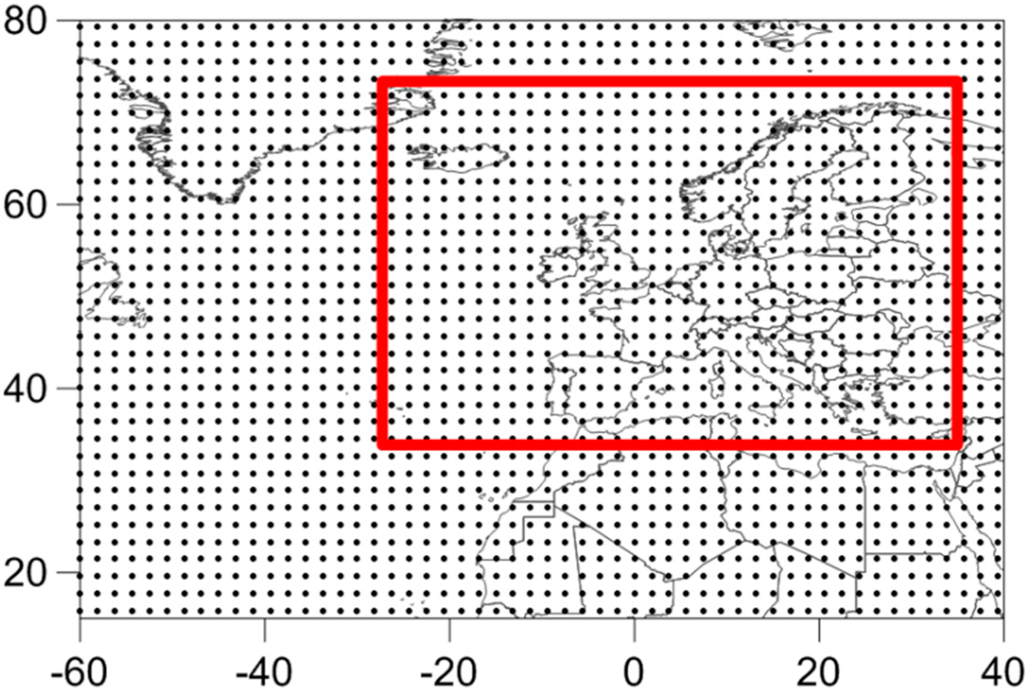
The data used to study the NAO pattern consist of winter (December–January–February) daily anomalies (the monthly climatology of the period studied is subtracted from the time series of each month) of the 500 hPa geopotential height field (gph500), simulated by the GCM ECHAM5/MPI for a present, 1971–2000 [16], and a future period, 2071–2100, based on the A1B SRES scenario [17]. Surface air temperature and precipitation winter daily data originate from the same model. The spatial resolution of the model is 1.875° × 1.875°. The area used to study the NAO pattern is defined by 60° W to 40° E and 15° N to 80° N and a smaller window over Europe is used for temperature and precipitation, as in 25° W to 34° E and 34° N to 72° N (Figure 1).
The ECHAM5/MPI model is a fifth-generation atmospheric General Circulation Model (GCM), developed at the Max Planck Institute for Meteorology (MPI), a recent version in a series of ECHAM models evolving originally from the weather prediction model of the European Centre for Medium Range Weather Forecasts (ECMWF). The particular model was chosen due to its documented capability of reproducing the NAO-related atmospheric circulation [10,18]. For further information on the model, refer to Roeckner et al. [19] and Jungclaus et al. [20].
2.2. Methods
2.2.1. Self-Organizing Maps
The main method used in this work to study NAO flavors is Self-Organizing Maps (SOM). SOM is a non-linear data analysis method that codifies large multivariate datasets onto a 2-dimensional array, where topological properties of input data are maintained. In other words, SOM is not only able to cluster the data, but to order the clusters as well. It is an Artificial Neural Network (ANN) technique of unsupervised learning, proposed in the 1980s by Kohonen [21,22] and used since then in a large number of different fields (medicine, biology, finance, speech recognition, text mining, image processing and other [23]), atmospheric sciences being one of them [24,25]. The methodology has proved useful in matters of weather and circulation pattern classification [26,27,28] and it is considered a good alternative, with several additional advantages to more traditional methods, such as Principal Component Analysis [10,29], Factor Analysis and k-means [30,31], Hierarchical Clustering [32], and others.
There are two main properties of the method, the self-organization, which refers to the ability of a simple algorithm to produce organization starting from possibly total disorder, and the topology conservation property, which means that similar input data belong to the same node or to neighboring ones [33]. Each node is defined by a weight vector of same size with the input data, a position in the array and the associated input data. The SOM algorithm starts with a random initialization, so that random values are chosen for the initial weight vectors. As a next step, each of the input data is attributed to its Best Matching Unit (BMU), according to a metric, which is usually the Euclidean distance. Then, the BMU is updated, becoming more similar to the input. Neighboring nodes are also updated—a property that makes SOM different from other clustering techniques as k-means [34]—according to the neighborhood radius size, which is linearly decreasing with time. The algorithm keeps returning to the start for as long as the clustering result keeps changing and it gets finalized when all input data have been classified to their BMU.
There is a number of choices that have to be made associated with the application of the SOMs. One of them is the size of the SOM array, which is usually chosen subjectively, according to the aim of each study. Here, aiming for a great degree of detail of the spatial variability of the NAO pattern, a large SOM array was chosen, equal to 10 × 10. Gibson et al. [35] also use large SOM configurations as they are found to generally improve the realism of the classification. SOM is a randomly initialized network, thus it gives a different clustering result every time it is implemented [36], although the conclusions drawn remain remarkably consistent. Nevertheless, it is highly recommended that multiple random runs are conducted and the one with the minimum errors should be chosen [10]. The two most frequently used errors to evaluate a SOM clustering result are the quantization and the topographical error. The first one measures the goodness of the neural network, thus how well it fits the input data. Therefore, the smallest the q-error, the better the clustering. Q-error is defined as follows:
where N is the number of data-vectors and is the BMU of the corresponding data-vector.
The topographical error is a measure of the topology preservation. It is the percentage of input data (in this case days) for which the second-best matching unit is an adjacent to the BMU SOM node. So the lower the topographic error, the better SOM preserves the topology [37]. The topographic error is calculated, as shown in Equation (2):
where equals 0 if vector’s first and second BMUs are adjacent SOM nodes and 1 if they are not.
In the present study, 10 random runs were performed and the best one according to the sum of the two aforementioned errors, was kept and analyzed. For the implementation of the SOM algorithm the R “kohonen package” [38] was used.
2.2.2. Defining the NAO Flavors
As a first step, Principal Component Analysis (PCA) was applied on the data of the reference period (1971–2000) in order to obtain a typical NAO spatial pattern as a prototype for comparison. According to many relevant studies, winter NAO is well represented by the first Empirical Orthogonal Factor (EOF1) of the sea-level pressure [5,39,40] or the geopotential height field at 500 hPa over North Atlantic [41,42].
After that, the SOM methodology was applied on the combined dataset of both reference and future periods. A large SOM array was used, in order to obtain a great degree of detail regarding the different longitudinal positions occupied by the two NAO action centers throughout the study periods. In particular, the SOM dimensions were chosen to be 10 × 10, resulting in 100 SOM nodes (a SOM node is analogous to a cluster in clustering techniques), representing characteristic atmospheric states extracted from the data. Then, the covariance between EOF1 and each of the 100 SOM nodes was calculated and the cases for which it was found to be higher/lower than one standard deviation, were characterized as “NAO-like nodes”, for positive (NAO+) and negative (NAO−) phase accordingly. For the rest of this study, only these NAO-like nodes are considered.
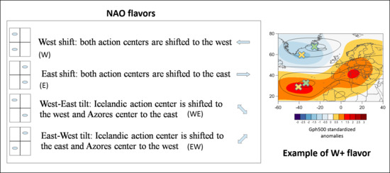
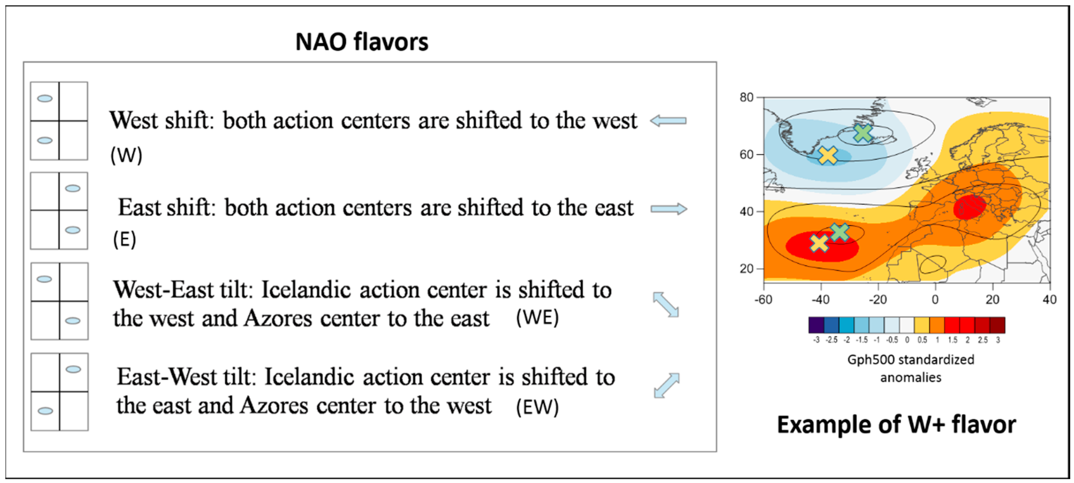
As a next step, each of the NAO-like nodes was compared to the EOF1 prototype as to the locations of the two centers of action. Certain variations of these locations were found, referred to as NAO flavors from now on, as each of the action centers, Icelandic Low and Azores High, can be located either west or east of the prototype defined by the EOF1. Therefore, the following categories of NAO flavors were obtained and the patterns related to NAO+ and NAO− were grouped respectively (see also Figure 2, where the NAO flavors are presented graphically in the left panel and a random day characterized by a W+ flavor is shown as an example in the right panel):
- West shift (W): both action centers are shifted to the west of the NAO prototype centers.
- West-east tilt (WE): the Icelandic center is shifted to the west and the Azores one to the east.
- East shift (E): both action centers are shifted to the east
- East-west tilt (EW): the NAO pattern is tilted, the Icelandic center is shifted to the east and the Azores one to the west.
Then, the longitudinal shift was measured as the horizontal distance between the centers of the EOF1 prototype and the centers of each flavor, for both the Icelandic Low and Azores High. Then the average of the two was calculated and attributed to each of the NAO flavors. This way, shifts were categorized in three groups: shorter than 10°, between 10 and 30° and longer than 30°.
At the last part of this study, composites of the days that belong to each of the NAO flavors were constructed and their statistical characteristics, such as frequency, persistence, and temporal trend of frequency (using the Mann-Kendall trend test) were analyzed. These composites were also used to study temperature and precipitation anomalies over Europe for each of the NAO flavors. The differences were tested for statistical significance at the 0.95 confidence level with the use of Student’s t-test.
3. Results
In this section, the results are presented in the following order: first, results related to atmospheric circulation, the NAO flavors, and their characteristics are shown. Then, the effects of these flavors on temperature and precipitation over Europe are presented with the use of composite maps and the statistical significant differences compared to their mean climate state are presented.
3.1. NAO Flavors
The EOF1 of the domain studied (presented with black contour lines in the map of the right panel of Figure 2) is a characteristic winter NAO pattern, with lower than average geopotential heights over Iceland and higher than average over the Azores Islands. All NAO-like patterns found in this study will be compared to this NAO-prototype pattern.
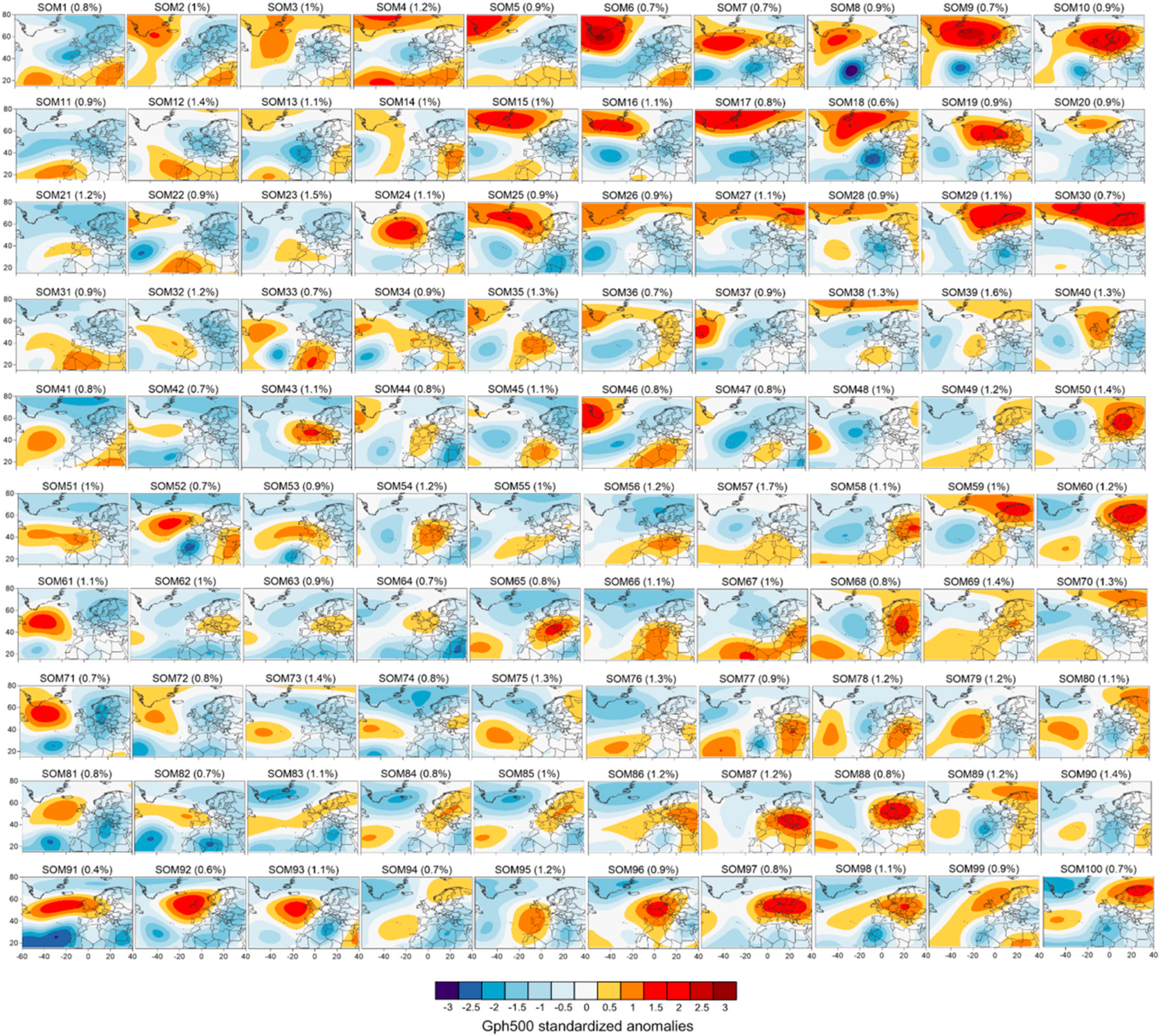
The results of the SOM application on the dataset under study are shown in the maps of Figure 3. There are 100 SOM nodes (10 × 10 array) representing characteristic atmospheric states of the 500 hPa geopotential height anomalies for winter. On top of each map, the number of the SOM node and its frequency for the studied period are noted.
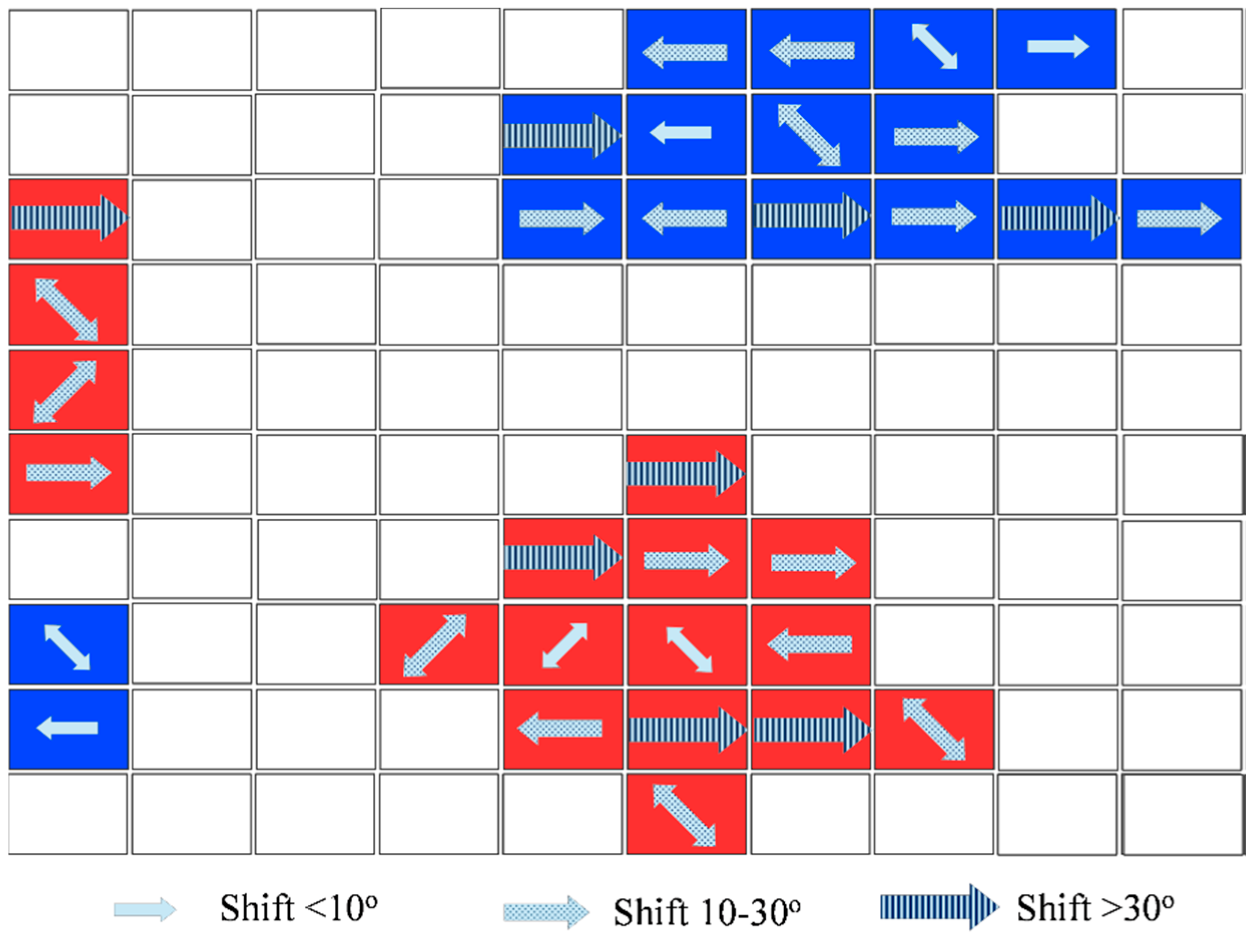
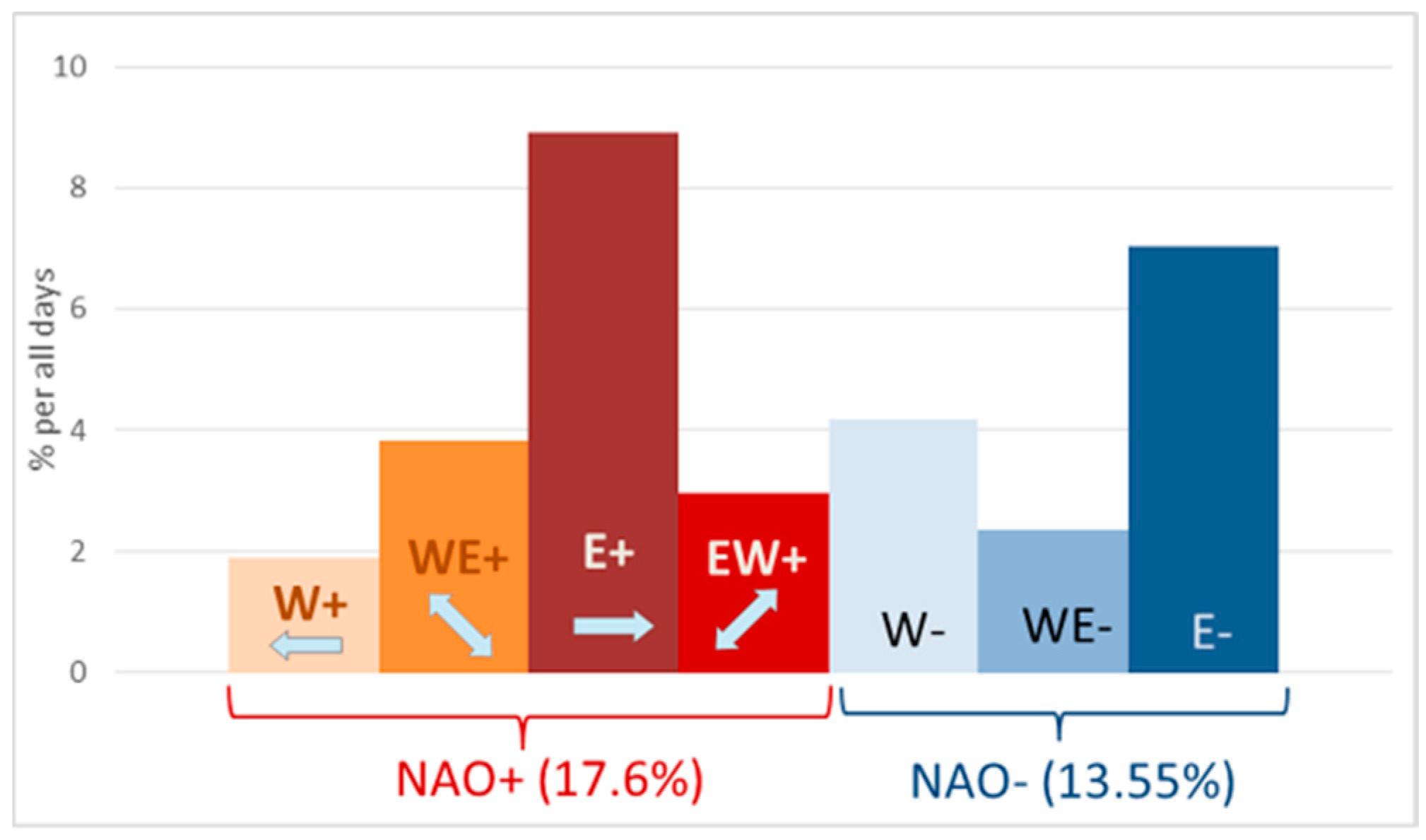
By calculating the covariance of the EOF1 with all the SOM nodes, 33 of the latter were found to be above/below the threshold of plus/minus one standard deviation and thus characterized as NAO-like nodes (presented in Figure 4 as coloured boxes), accounting for 31% of the days of the study period. Among these days, 17.6% are NAO+ and 13.5% NAO− (red and blue boxes in Figure 4, respectively). Examining the present and future period separately, NAO days are more frequent in the future (+1.6%), a fact that is due to an increase of NAO− days from 12.7% in 1971–2000 to 14.4% in 2071–2100. NAO+ days are slightly decreasing (−0.2%). The overall trend of the frequency of the NAO days is positive, but not statistically significant. In a comparison with reanalysis data (NCEP/NCAR, not shown), the model seems to overestimate (underestimate) the frequency of occurrence of NAO+ (NAO−) days.
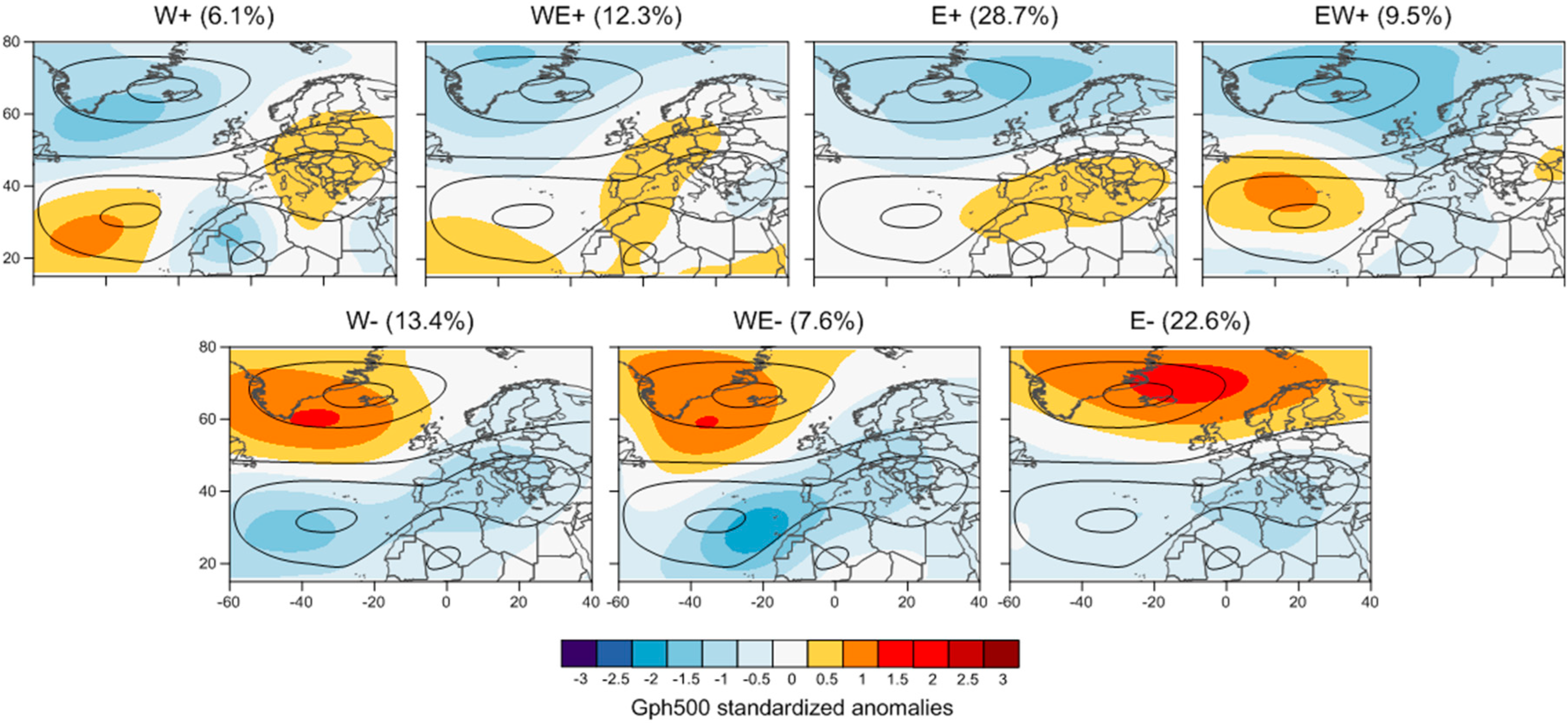
In Figure 4, one can clearly see the topological ordering property of the SOM methodology, with positive (red coloured boxes) and negative NAO phases (blue coloured boxes) well separated in the SOM array and each group of nodes occupying a different part of it. At the next step, the shifts of the NAO action centers were measured, in means of differences in longitudinal degrees from the EOF1-based prototype. These shifts, or NAO flavors, are presented with arrows in Figure 4 and their frequency distributions among the days of the periods studied are shown in Figure 5. Their statistical characteristics are summarized in Table 1. The composites of geopotential height anomalies for each of the flavors are presented in Figure 6. When NAO is in its positive phase, the most frequent flavor is the east one (E+), occurring in 29% of NAO days and in 50% of NAO+ days, in particular. This flavor, apart from being the most dominant, is also characterized by positive frequency trends in both periods, which is statistically significant only for the future one (Table 1). Moreover, it is the most persistent flavor with an average occurrence of 3 days and a maximum occurrence of 13 days in a row. The WE+ flavor is also exhibiting a statistical significant positive trend during the future period. On the other hand, the W+ and EW+ flavors seem to increase in persistence in the future period compared to the present. For the negative phase of NAO, the most frequent and persistent flavor is again the east one (E−), with a frequency of 23% among NAO days and 52% among NAO− days and an average (maximum) persistence of 3.4 (11) days. The west flavor (W−) follows, with an occurrence of 13% among NAO days.
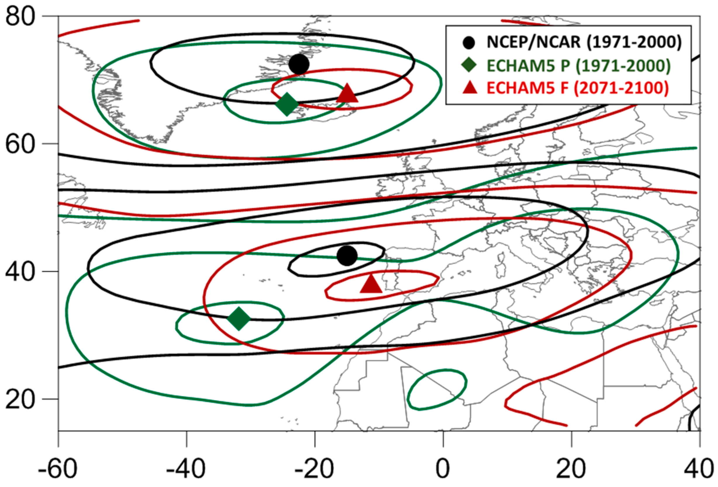
When compared to reanalysis data, the model overestimates the frequency of E+ days that nevertheless remains the most frequent NAO+ flavor in all datasets examined. It also overestimates the frequency of E− and underestimates those of all other flavors for NAO−. This tendency can be partly explained by the fact that the centers of the NAO prototype for the model’s reference period are located more to the west, compared to the ones in the reanalysis data, as seen in Figure 7. Nevertheless, in the model’s future period, there is still a displacement of the NAO centers farther to the east, both compared to the model’s present period and the reanalysis data.
The NAO flavors can also be examined regarding the shift of the two action centers. As seen in Table 2, for both NAO+ and NAO−, the two action centers are more frequently shifted to the east. For NAO+, the Icelandic Low is, in average, located 23° east of the EOF1 prototype, while the Azores High has an even larger average displacement of 35° east. For NAO−, the Icelandic Low (Azores High) shows an average east displacement of 17° (26°). In other words, the east shift is dominant for both action centers and for both NAO phases. A more detailed description of the shifts for each action center is given in Table 2.
3.2. NAO Flavors and Temperature over Europe
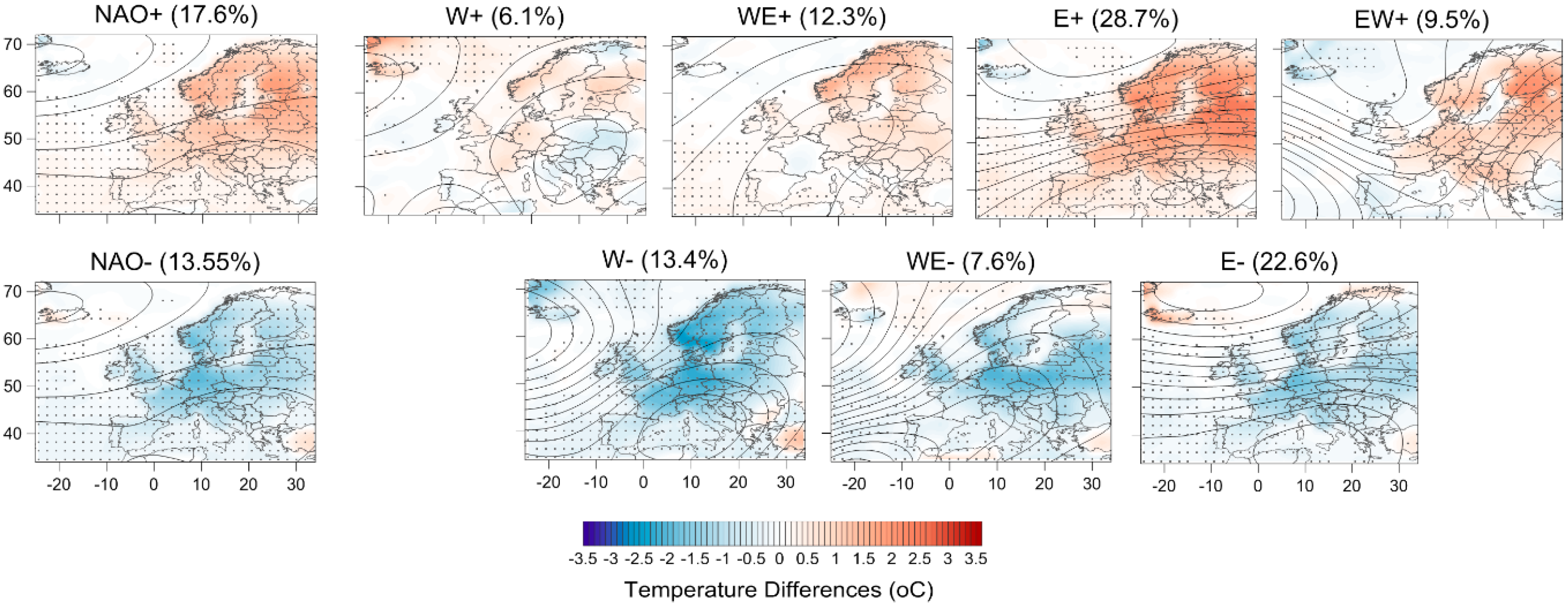
Here, the NAO flavors discussed in the previous session are examined with respect to their implications on winter surface air temperature over Europe. The results are presented in Figure 8 and Figure 9, in the form of differences from the mean state. The temperature differences during NAO+ and NAO-, regardless of the flavor, are also shown for comparison.
As expected, during NAO+, warmer temperature prevail over central and northern Europe, with the highest values over the northeastern regions, such as Finland and the Baltic countries. The North Atlantic is not much affected, with the exception of Iceland and a small area around it, where temperature is lower than average during NAO+ days. For NAO-, the situation is more or less the opposite than the one just described, with cooler than average temperatures over most of Europe. The lowest temperatures are found over central Europe and particularly in Germany.
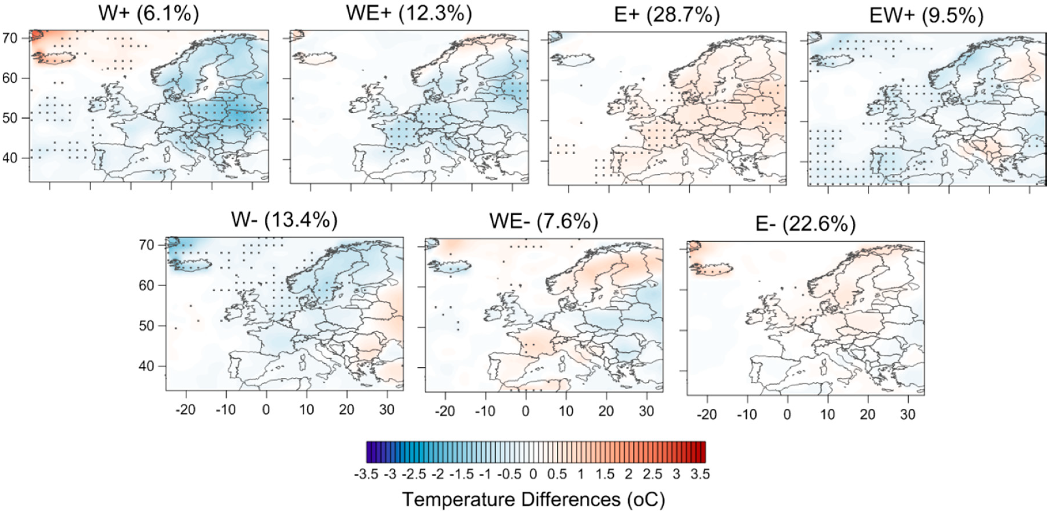
This is the general situation during NAO positive and negative phases. However, there are differences in how the NAO flavors, as defined in this study, contribute to the response of the temperature regime over Europe. This can be seen in the maps of Figure 8 (differences between average temperature and temperature for the days that are characterized by each NAO flavor), but also in those of Figure 9, where the differences are calculated from the temperature during days of positive (and negative) NAO phase.
Starting with NAO+, the west flavor (W+) gives warmer temperatures over North Europe as NAO+ in general, but they are less extended into Scandinavia and Eastern Europe and are mostly not statistically significant. On the other hand, statistically significant warmer temperatures are found over Iceland and the farthest north Atlantic, a situation occurring only during this particular NAO+ flavor. Southern and Eastern Europe are dominated by cooler than average temperatures, however the differences are not statistically significant. The WE+ flavor is related to warmer temperatures over most of eastern and northern Europe, with larger, and statistical significant, values over most parts of Scandinavia. Small negative differences are found over France and northern Atlantic. When the E+ flavor dominates, we see the largest and most significant positive temperature differences, spread all over Europe. The highest winter temperatures are found during this flavor and, in particular, over northeastern Europe, while there are cooler than average temperatures over Iceland. The EW+ flavor is characterized by warmer temperatures over large parts of Europe, apart from the Iberian Peninsula, the UK, and the farthest eastern regions. The highest values are found over Finland and the Baltic countries.
Therefore, E+ is the flavor that contributes the most to the expected NAO+ response of milder winters over Europe, and it also exhibits, as mentioned above, a positive temporal trend (though not statistically significant). This contribution can also be clearly seen in Figure 9, as E+ is the only flavor with temperatures higher than those during all NAO+ days. In certain regions, including France, the Iberian Peninsula, and the UK, the differences exceeding the NAO+ average effects are statistically significant. The WE+ flavor is characterized by a statistically significant positive trend of its frequency in the future period (equal to an increase in frequency of 0.3% per year), which means more common occurrence of warmer temperatures over central and northeastern Europe.
In regard to NAO, there are slightly different spatial patterns of temperature during the NAO flavors. The W− is the one with the more spread and largest negative differences, with the lowest values located over North Sea and Scandinavia. When the pattern occurs in a WE− flavor, the coolest temperatures are found over central Europe, and particularly north Germany and Poland. During the E− flavor, south and southeastern Europe present lower temperatures than for all NAO-days.
3.3. NAO Flavors and Precipitation over Europe
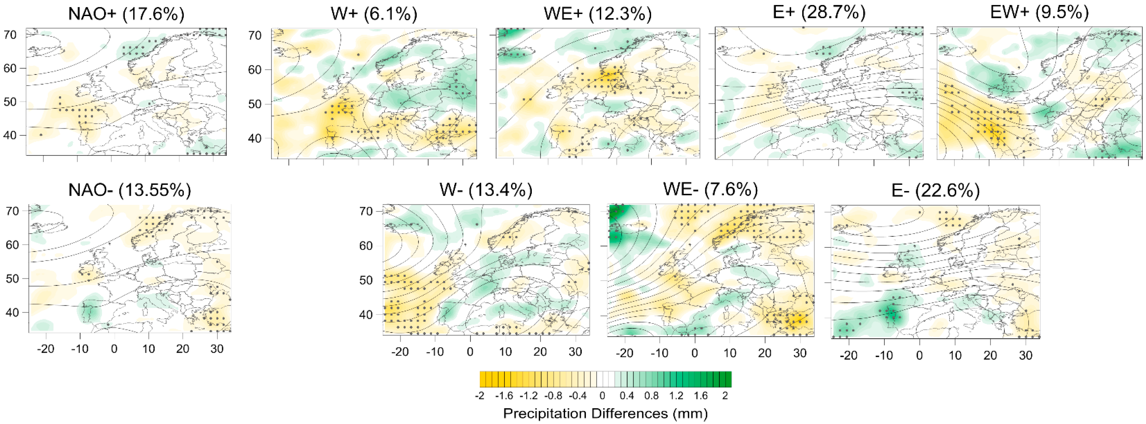
Regarding the response of precipitation to the NAO flavors, the spatial patterns are not as coherent as the ones for temperature, due to its more regional/localized character, but there still exist regions where the effect of certain flavors is prominent. Such cases are connected to areas where frontal rainfall can be facilitated or hindered by the atmospheric configuration during the various NAO flavors.
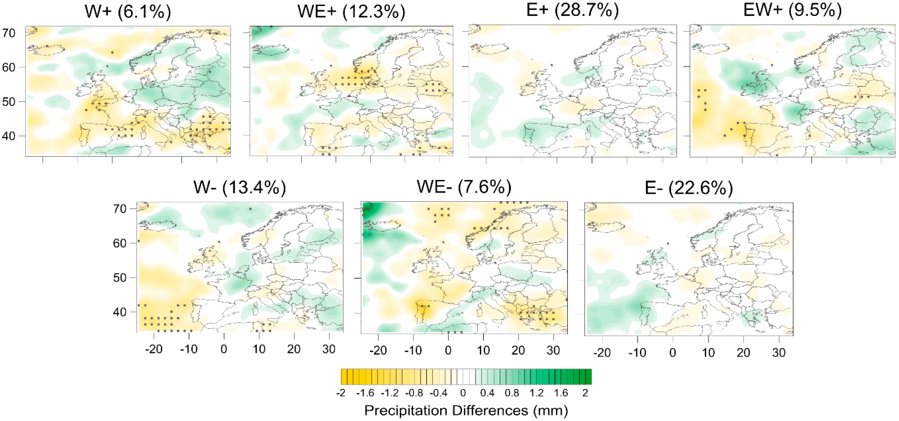
During NAO+, there is decreased precipitation over the western part of Europe, especially north of Spain, over the Biscay Bay, and the English Channel (Figure 10). Increased precipitation is found over north of Norway and in the southeastern Mediterranean. Comparing the general NAO+ conditions with those occurring during the various flavors, there are some clear differences in precipitation amounts and their statistical significance (as seen in Figure 10 and Figure 11). For instance, during W+, there are many more regions exhibiting a statistically significant decrease in precipitation. Other than western Europe, these areas include the northern coasts of the Mediterranean and southeastern Europe. Over those areas, during days with the W+ flavor, these anomalies are statistically significant in comparison to average NAO+ days. On the other hand, precipitation is significantly increased over the northeastern part of the domain, something not seen when averaging over all NAO+ days. During the WE+ flavor, there is a significant decrease of precipitation over the North Sea and southern Scandinavia, as well as southwestern Mediterranean, and small parts of eastern Europe. The statistically increased precipitation over northern parts of the domain that occurs during NAO+, is mainly a contribution of the WE+ flavor for Iceland, and of the E+ flavor for the western locations.
During NAO−, there is a dipole of positive and negative precipitation differences over western Iberian Peninsula and western UK, respectively. There are not so many statistically significant differences for all NAO− days, but many more for certain flavors in different regions. During W−, a significant decrease is seen over the southern part of the Atlantic, while for WE− this is the case for the northern regions of the domain and for the southeastern as well. The E− flavor is bringing statistically significant more precipitation over the southwestern part of the domain, including the Iberian and the Biscay Bay. In this case, the more pronounced, compared to all other flavors, westerly circulation over this region allows for more low-pressure systems that bring excess precipitation.
4. Discussion
Our approach in this paper is that of avoiding the use of a point-based NAO index, but instead, defining different spatial flavors, according to the positions that the NAO centers of action occupy each time, with the use of SOMs. As underlined in recent impact-related studies, (climate–streamflow links in Steirou et al. [43]; northern European sea level in Chafik et al. [44]; influence of weather regimes on the energy sector in van der Wiel et al. [45]), the need for a non-station based index is pronounced in order to fully capture the spatial configuration of the NAO mode. Studies in the past have focused on defining different flavors of ENSO [46] or of Indian Ocean Dipole events [47] with SOMs, or with complex climate networks [48]. The NAO pattern has received a lot of attention as well, as particularly for the North Atlantic, the sensitivity of teleconnections’ structure to a slight shift in the base point or in the sign of their primary action centers can be fairly large due to their nonlinear characteristics [49]. Several previous studies have tried to tackle the non-stationarity of the NAO pattern, using for instance, regions rather than points [10], a seasonally and geographically mobile index [50], or different techniques trying to include the interplay of the NAO actions centers between them [51] and with other teleconnection patterns, such as the East Atlantic and the Scandinavian pattern [52,53].
Therefore, in this paper, we argue and show that NAO flavors have different local effects on winter temperature and precipitation over Europe. Castro-Díez et al. [54] also state that winter temperatures in southern Europe are not only sensitive to the phase of the NAO, but also to the exact location of the NAO centers of action. As indicated by Rust et al. [55], the NAO has explanatory potential for temperature in wide areas of Europe that is related to circulation anomalies, particularly in winter. As the advection of maritime or continental air masses dominates in winter, the specific location of the NAO centers is of great importance as to where exactly those masses will be transported, leading to warmer or colder temperatures and excess or decreased precipitation amounts. In a recent study, Kim et al. [56] pointed out that the conventional NAO definition could not account for pronounced differences found in sea surface temperature over North Atlantic, whereas a west-centered NAO pattern and the corresponding index lead to significant improvements. This was the case for the winter of 2008, due to the fact that the large-scale atmospheric anomalies were centered in the western North Atlantic setting a strong pressure gradient over the Labrador Sea [56]. As NAO has been recognized as a major driver of the Atlantic Meridional Overturning Circulation [57], but can also be partially driven by it on interdecadal timescales [58], the better understanding of their nonlinear, nonstationary interactions is important, and our spatial NAO flavors approach, can contribute to this direction. Moreover, according to Vicente-Serrano & López-Moreno [59], the non-stationarity in the relationship between NAO and European precipitation is associated with the multidecadal variability in the locations of the NAO’s centers of action. Yao & Luo [60] examined the difference between an eastern and a western-type of NAO and their impacts on European temperature and precipitation and their results show that there are regionally different responses of these variables. In their case, only the location of the northern NAO center of action (Icelandic Low) was considered, while we chose to examine the relative position of the southern one (Azores High) as well.
5. Conclusions
The main conclusions of this study can be summarized in the following points:
- NAO is not a stationary pattern. Its centers of action exhibit different spatial variations, affecting temperature and precipitation regimes in Europe in different ways. This is why the definition of NAO flavors is a useful approach. It is important to mention that the NAO flavors should be defined from scratch each time for different datasets and time-periods. The ones presented here regard the winter field of geopotential height at 500hPa for 1971–2000 and 2071–2100 in the ECHAM5 model. Most of the NAO flavors found in these simulations do not change significantly in frequency and persistence at the end of the 21st century. However, they do have significant implications for temperature and precipitation over Europe, that differ from the typical NAO effects, when all NAO+ or NAO− days are taken under consideration.
- The model identifies the centers of NAO for the present period to the west of those in the reanalysis data, while the centers for the future period present a significant displacement to the east (mainly compared to the model present period, but also to the reanalysis). This is in agreement with several studies documenting eastward shifts of the NAO centers of action, in both observed data [61] and in experiments with general circulation models of different levels of complexity [9,62,63]. According to Peterson et al. [64], it is the strength of the mean westerly flow that drives the changes in the spatial structure of interannual NAO variability in a nonlinear way. In agreement with the above statements, we find that the most frequent NAO flavor is an east shift, for both positive and negative NAO.
- The typical warmer winter temperatures over Europe are mainly found to be occurring during the E+ flavor. Yao & Luo [60] also reached similar conclusions, as an NAO pattern with its northern center of action located to the east of 10° W of longitude has a wider and stronger imprint on European temperature than when it is located in a westerly position. Colder winter temperatures are found over northern Europe, mostly as a response to the W− flavor, while this is the case for Eastern Europe when WE− is dominant.
- Precipitation is spatially more incoherent compared to temperature and this is reflected in our results. During the W+ and EW+ flavors, precipitation amounts are significantly lower in western Europe, while this is the case for Scandinavia when W− and WE− flavors are dominant. Significantly more precipitation is occurring over northeastern Europe mainly with W+, and with E- over southwestern Europe. For more detailed and localized effects of the NAO flavors on regional precipitation, one should look at the different SOMs that comprise those flavors, instead of only looking at their composites, as this way, regional differences even out.
Future work is planned in order for the proposed methodology to be applied on ensembles of different models and runs so that robust results can be obtained, regarding not only the natural variability of the NAO pattern, but also differences in the context of a changing climate. The present study should be seen as a methodological one, as it is an experiment carried out using only one climate model. Moreover, the same methodology is being used to define summer NAO flavors and also to examine the effects of the flavors on other climate variables, such as winds and storm tracks, as well as extreme events. The interactions of NAO flavors with North Atlantic sea-surface temperatures are also under examination. Another interesting direction is to further analyze the different NAO patterns that present split action centers and try to understand their drivers.
Author Contributions
All authors conceived the idea of the study. E.R. did the data analysis and wrote the original draft manuscript. All authors contributed to the discussion and interpretation of the results and the editing of the manuscript. All authors have read and agreed to the published version of the manuscript.
Funding
E.R. was financially supported by the German Academic Exchange Service–DAAD (grant 91580150) and the German Federal Ministry of Education and Research–BMBF (grant 01LP1611A).
Acknowledgments
The authors are grateful to the Max Planck Institute for Meteorology and the German Climate Computing Center (DKRZ) that provide the ECHAM5 model data freely to the public. The authors would also like to thank four anonymous reviewers for their constructive comments and suggestions that improved the manuscript.
Conflicts of Interest
The authors declare no conflict of interest.
References
- Hurrell, J.W. Decadal trends in the North Atlantic Oscillation: Regional temperatures and precipitation. Science 1995, 269, 676–679. [Google Scholar] [CrossRef] [PubMed] [Green Version]
- Wibig, J. Precipitation in Europe in relation to circulation patterns at the 500 hPa level. Int. J. Climatol. 1999, 19, 253–269. [Google Scholar] [CrossRef]
- Scaife, A.A.; Folland, C.K.; Alexander, L.V.; Moberg, A.; Knight, J.R. European climate extremes and the North Atlantic Oscillation. J. Clim. 2008, 21, 72–83. [Google Scholar] [CrossRef]
- Scaife, A.A.; Knight, J.R.; Vallis, G.K.; Folland, C.K. A stratospheric influence on the winter NAO and North Atlantic surface climate. Geophys. Res. Lett. 2005, 32. [Google Scholar] [CrossRef] [Green Version]
- Hurrell, J.W.; Kushnir, Y.; Ottersen, G.; Visbeck, M. An overview of the North Atlantic Oscillation. Geophys. Monogr. Am. Geophys. Union 2003, 134, 1–36. [Google Scholar]
- Wang, L.; Ting, M.; Kushner, P.J. A robust empirical seasonal prediction of winter NAO and surface climate. Sci. Rep. 2017, 7, 279. [Google Scholar] [CrossRef] [Green Version]
- Rogers, J.C. The Association between the North Atlantic Oscillation and the Southern Oscillation in the Northern Hemisphere. Mon. Weather Rev. 1984, 112, 1999–2015. [Google Scholar] [CrossRef]
- Hilmer, M.; Jung, T. Evidence for a recent change in the link between the North Atlantic Oscillation and Arctic Sea ice export. Geophys. Res. Lett. 2000, 27, 989–992. [Google Scholar] [CrossRef] [Green Version]
- Ulbrich, U.; Christoph, M. A shift of the NAO and increasing storm track activity over Europe due to anthropogenic greenhouse gas forcing. Clim. Dyn. 1999, 15, 551–559. [Google Scholar] [CrossRef]
- Rousi, Ε.; Anagnostopoulou, C.; Tolika, K.; Maheras, P. Representing teleconnection patterns over Europe: A comparison of SOM and PCA methods. Atmos. Res. 2015, 152, 123–137. [Google Scholar] [CrossRef]
- Rousi, E.; Ulbrich, U.; Rust, H.W.; Anagnostolpoulou, C. An NAO climatology in reanalysis data with the use of self-organizing maps. In Perspectives on Atmospheric Sciences; Karacostas, T., Bais, A., Nastos, P.T., Eds.; Springer Atmospheric Sciences; Springer: Cham, Switzerland, 2017; pp. 719–724. [Google Scholar]
- Luo, D.; Gong, T. A possible mechanism for the eastward shift of interannual NAO action centers in last three decades. Geophys. Res. Lett. 2006, 33. [Google Scholar] [CrossRef]
- Cattiaux, J.; Vautard, R.; Cassou, C.; Yiou, P.; Masson-Delmotte, V.; Codron, F. Winter 2010 in Europe: A cold extreme in a warming climate. Geophys. Res. Lett. 2010, 37. [Google Scholar] [CrossRef] [Green Version]
- Luo, D.; Chen, X.; Feldstein, S.B. Linear and nonlinear dynamics of North Atlantic Oscillations: A new thinking of symmetry breaking. J. Atmos. Sci. 2018, 75, 1955–1977. [Google Scholar] [CrossRef]
- Nigam, S.; Baxter, S. Teleconnections. In Encyclopedia of Atmospheric Sciences, 2nd ed.; North, G., Ed.; Elsevier Science: Amsterdam, The Netherlands, 2015; pp. 90–109. [Google Scholar]
- Roeckner, E. IPCC MPI-ECHAM5_T63L31 MPI-OM_GR1. 5L40 20C3M_All Run No. 3: Atmosphere 6 HOUR Values MPImet/MaD Germany; World Data Center for Climate: Hamburg, Germany, 2005. [Google Scholar]
- Roeckner, E.; Lautenschlager, M.; Schneider, H. IPCC-AR4 MPIECHAM5_T63L31 MPI-OM_GR1.5 L40 SRESA1B Run No.3: Atmosphere 6 HOUR Values MPImet/MaD Germany; World Data Center for Climate: Hamburg, Germany, 2006. [Google Scholar]
- Stoner, A.M.K.; Hayhoe, K.; Wuebbles, D.J. Assessing general circulation model simulations of atmospheric teleconnection patterns. J. Clim. 2009, 22, 4348–4372. [Google Scholar] [CrossRef]
- Roeckner, E.; Bäuml, G.; Bonaventura, L.; Brokopf, R.; Esch, M.; Giorgetta, M.; Hagemann, S.; Kirchner, I.; Kornblueh, L.; Manzini, E.; et al. The Atmospheric General Circulation Model EHAMPart I: Model Description; MPI für Meteorologie: Hamburg, Germany, 2003. [Google Scholar]
- Jungclaus, J.H.; Keenlyside, N.; Botzet, M.; Haak, H.; Luo, J.J.; Latif, M.; Marotzke, J.; Mikolajewicz, U.; Roeckner, E. Ocean circulation and tropical variability in the coupled model ECHAM5/MPI-OM. J. Clim. 2006, 19, 3952–3972. [Google Scholar] [CrossRef] [Green Version]
- Kohonen, T. Self-organized formation of topologically correct feature maps. Biol. Cybern. 1982, 43, 59–69. [Google Scholar] [CrossRef]
- Kohonen, T. Self-Organizing Maps; Springer: Berlin/Heidelberg, Germany, 2001. [Google Scholar]
- Miljković, D. Brief review of self-organizing maps. In Proceedings of the 2017 40th International Convention on Information and Communication Technology, Electronics and Microelectronics (MIPRO), Opatija, Croatia, 22–26 May 2017; pp. 1061–1066. [Google Scholar]
- Cavazos, T. Large-scale circulation anomalies conducive to extreme precipitation events and derivation of daily rainfall in Northeastern Mexico and Southeastern Texas. J. Clim. 1999, 12, 1506–1523. [Google Scholar] [CrossRef]
- Hewitson, B.; Crane, R. Self-organizing maps: Applications to synoptic climatology. Clim. Res. 2002, 22, 13–26. [Google Scholar] [CrossRef]
- Reusch, D.B.; Alley, R.B.; Hewitson, B.C. North Atlantic climate variability from a self-organizing map perspective. J. Geophys. Res. Atmos. 2007, 112. [Google Scholar] [CrossRef]
- Schuenemann, K.C.; Cassano, J.J.; Finnis, J. Synoptic forcing of precipitation over Greenland: Climatology for 1961–1999. J. Hydrometeorol. 2009, 10, 60–78. [Google Scholar] [CrossRef]
- Rousi, E.; Mimis, A.; Stamou, M.; Anagnostopoulou, C. Classification of circulation types over Eastern mediterranean using a self-organizing map approach. J. Maps 2014, 10, 232–237. [Google Scholar] [CrossRef] [Green Version]
- Reusch, D.B.; Alley, R.B.; Hewitson, B.C. Relative performance of self-organizing maps and principle component analysis in pattern extraction from synthetic climatological data. Polar Geogr. 2005, 29, 188–212. [Google Scholar] [CrossRef]
- Kiang, M.Y.; Kumar, A. An evaluation of self-organizing map networks as a robust alternative to factor analysis in data mining applications. Inf. Syst. Res. 2001, 12, 177–194. [Google Scholar] [CrossRef]
- Philippopoulos, K.; Deligiorgi, D.; Kouroupetroglou, G. Performance comparison of self-organizing maps and k-means clustering techniques for atmospheric circulation classification. Int. J. Energy Environ. 2014, 8, 171–180. [Google Scholar]
- Abbas, O. Comparisons between data clustering algorithms. Int. Arab J. Inf. Technol. 2008, 5, 320–325. [Google Scholar]
- Cottrell, M.; Fort, J.; Pagès, G. Theoretical aspects of the SOM algorithm. Neurocomputing 1998, 21, 119–138. [Google Scholar] [CrossRef] [Green Version]
- Kaski, S. Data exploration using self-organizing maps. In Acta Polytechnica Scandinavica: Mathematics, Computing and Management in Engineering Series No. 82; Finnish Academy of Technology: Espoo, Finland, 1997. [Google Scholar]
- Gibson, P.B.; Uotila, P.; Perkins-Kirkpatrick, S.E.; Alexander, L.V.; Pitman, A.J. Evaluating synoptic systems in the CMIP5 climate models over the Australian region. Clim. Dyn. 2016, 47, 2235–2251. [Google Scholar] [CrossRef]
- Fort, J.C.; Letremy, P.; Cottrell, M. Advantages and drawbacks of the Batch Kohonen algorithm. In Proceedings of the European Symposium on Artificial Neural Networks ESANN, Bruges, Belgium, 24–26 April 2002; pp. 223–230. [Google Scholar]
- Uriarte, E.A.; Martín, F.D. Topology preservation in SOM. Int. J. Appl. Math. Comput. Sci. 2005, 1, 19–22. [Google Scholar]
- Wehrens, R.; Kruisselbrink, J. Flexible self-organizing maps in kohonen 3.0. J. Stat. Softw. 2018, 87, 1–18. [Google Scholar] [CrossRef] [Green Version]
- Barnston, A.G.; Livezey, R.E. Classification, seasonality and persistence of low-frequency atmospheric circulation patterns. Mon. Weather Rev. 1987, 115, 1083–1126. [Google Scholar] [CrossRef]
- Glowienka-Hense, R. The North Atlantic Oscillation in the Atlantic-European SLP. Tellus A 1990, 42, 497–507. [Google Scholar] [CrossRef]
- Van Loon, H.; Rogers, J.C. The seesaw in winter temperatures between Greenland and Northern Europe. Part I: General description. Mon. Weather Rev. 1978, 106, 296–310. [Google Scholar] [CrossRef] [Green Version]
- Wallace, J.M.; Gutzler, D.S. Teleconnections in the geopotential height field during the Northern Hemisphere winter. Mon. Weather Rev. 1981, 109, 784–812. [Google Scholar] [CrossRef]
- Steirou, E.; Gerlitz, L.; Apel, H.; Merz, B. Links between large-scale circulation patterns and streamflow in Central Europe: A review. J. Hydrol. 2017, 549, 484–500. [Google Scholar] [CrossRef]
- Chafik, L.; Nilsen, J.E.O.; Dangendorf, S. Impact of North Atlantic teleconnection patterns on Northern European sea level. J. Mar. Sci. Eng. 2017, 5, 43. [Google Scholar] [CrossRef] [Green Version]
- Van Der Wiel, K.; Bloomfield, H.C.; Lee, R.W.; Stoop, L.P.; Blackport, R.; Screen, J.A.; Selten, F.M. The influence of weather regimes on European renewable energy production and demand. Environ. Res. Lett. 2019, 14, 094010. [Google Scholar] [CrossRef]
- Johnson, N.C. How many ENSO flavors can we distinguish? J. Clim. 2013, 26, 4816–4827. [Google Scholar] [CrossRef]
- Verdon-Kidd, D.C. On the classification of different flavours of Indian Ocean Dipole events. Int. J. Clim. 2018, 38, 4924–4937. [Google Scholar] [CrossRef]
- Wiedermann, M.; Radebach, A.; Donges, J.F.; Kurths, J.; Donner, R.V. A climate network-based index to discriminate different types of El Niño and La Niña. Geophys. Res. Lett. 2016, 43, 7176–7185. [Google Scholar] [CrossRef] [Green Version]
- Chen, W.Y.; Dool, H.V.D. Sensitivity of teleconnection patterns to the sign of their primary action center. Mon. Weather Rev. 2003, 131, 2885–2899. [Google Scholar] [CrossRef]
- Portis, D.H.; Walsh, J.E.; El Hamly, M.; Lamb, P.J. Seasonality of the North Atlantic Oscillation. J. Clim. 2001, 14, 2069–2078. [Google Scholar] [CrossRef]
- Hameed, S.; Piontkovski, S. The dominant influence of the Icelandic Low on the position of the Gulf Stream northwall. Geophys. Res. Lett. 2004, 31, 1998–2001. [Google Scholar] [CrossRef]
- Moore, G.W.K.; Renfrew, I.A.; Pickart, R.S. Multidecadal mobility of the North Atlantic Oscillation. J. Clim. 2013, 26, 2453–2466. [Google Scholar] [CrossRef] [Green Version]
- Zubiate, L.; Mcdermott, F.; Malley, M.O. Spatial variability in winter NAO—Wind speed relationships in western Europe linked to concomitant states of the East Atlantic and Scandinavian patterns. Q. J. R. Meteorol. Soc. 2017, 143, 552–562. [Google Scholar] [CrossRef] [Green Version]
- Castro-Díez, Y.; Pozo-Vazquez, D.; Rodrigo, F.S.; Esteban-Parra, M.J. NAO and winter temperature variability in southern Europe. Geophys. Res. Lett. 2002, 29. [Google Scholar] [CrossRef]
- Rust, H.W.; Richling, A.; Bissolli, P.; Ulbrich, U. Linking teleconnection patterns to European temperature—A multiple linear regression model. Meteorol. Z. 2015, 24, 411–423. [Google Scholar] [CrossRef]
- Kim, W.M.; Yeager, S.; Chang, P.; Danabasoglu, G. Atmospheric conditions associated with Labrador Sea deep convection: New insights from a case study of the 2006/07 and 2007/08 winters. J. Clim. 2016, 29, 5281–5297. [Google Scholar] [CrossRef]
- Delworth, T.L.; Zeng, F. The impact of the North Atlantic Oscillation on climate through its influence on the Atlantic meridional overturning circulation. J. Clim. 2016, 29, 941–962. [Google Scholar] [CrossRef]
- Caesar, A.L.; Rahmstorf, S.; Robinson, A.; Feulner, G.; Saba, V. Title: Observed fingerprint of a weakening Atlantic Ocean overturning circulation. Nature 2018, 556, 191–196. [Google Scholar] [CrossRef]
- Vicente-Serrano, S.M.; López-Moreno, J.I. Nonstationary influence of the North Atlantic Oscillation on European precipitation. J. Geophys. Res. Space Phys. 2008, 113. [Google Scholar] [CrossRef]
- Yao, Y.; Luo, D. Relationship between zonal position of the North Atlantic Oscillation and Euro-Atlantic blocking events and its possible effect on the weather over Europe. Sci. China Earth Sci. 2014, 57, 2628–2636. [Google Scholar] [CrossRef]
- Jung, T. The North Atlantic Oscillation: Variability and Interactions with the North Atlantic Ocean and Arctic Sea Ice; Christian-Albrechts-Universität: Kiel, Germany, 2000. [Google Scholar]
- Peterson, K.A.; Derome, J.; Greatbatch, R.J.; Lu, J.; Lin, H. Hindcasting the NAO using diabatic forcing of a simple AGCM. Geophys. Res. Lett. 2002, 29, 50–51. [Google Scholar] [CrossRef]
- Jung, T.; Hilmer, M.; Ruprecht, E.; Kleppek, S.; Gulev, S.K.; Zolina, O. Characteristics of the recent eastward shift of interannual NAO variability. J. Clim. 2003, 16, 3371–3382. [Google Scholar] [CrossRef] [Green Version]
- Peterson, K.A.; Lu, J.; Greatbatch, R.J. Evidence of nonlinear dynamics in the eastward shift of the NAO. Geophys. Res. Lett. 2003, 30. [Google Scholar] [CrossRef]
Figure 1.
Area of study. The large domain was used for the gph500 analysis of the North Atlantic Oscillation (NAO) and the small one (within the red box) for temperature and precipitation over Europe.
Figure 1.
Area of study. The large domain was used for the gph500 analysis of the North Atlantic Oscillation (NAO) and the small one (within the red box) for temperature and precipitation over Europe.

Figure 2.
Description of the NAO flavors. On the left panel, the flavors are explained in terms of shifts and tilts of the NAO action centers compared to the position of the EOF prototype. On the right panel, a random day characterized by a westerly shifted NAO+ flavor is presented. Coloured contours represent the 500 hPa geopotential height anomalies for this day and black contour lines the EOF1 anomalies. Green crosses represent the NAO centers of the EOF1 and yellow crosses the centers of this particular day. The longitudinal shift is then calculated, as the horizontal difference of the two corresponding centers in degrees of longitude (°).

Figure 3.
The 10 × 10 Self-Organizing Maps (SOM) array of winter gph500 standardized anomalies for the periods 1971–2000 and 2071–2100. The frequency of occurrence of each SOM is shown in parenthesis on top of each map. These SOMs are used in the following step to define NAO-like nodes and are grouped together to form the NAO flavors according to relative location of the action centers to the EOF1 NAO-prototype.

Figure 4.
Positive (red) and negative (blue) NAO phases for each of the SOMs of Figure 3. NAO flavors and quantification (in longitudinal degrees as the average of the shifts of the two action centers for each flavor) of the shift for each case are shown with arrows.
Figure 4.
Positive (red) and negative (blue) NAO phases for each of the SOMs of Figure 3. NAO flavors and quantification (in longitudinal degrees as the average of the shifts of the two action centers for each flavor) of the shift for each case are shown with arrows.

Figure 5.
Frequency distribution of NAO flavors (percentage over all days).

Figure 6.
SOM composites of gph500 standardized anomalies for each of the NAO flavors and their frequency (per NAO days) in both periods studied for NAO+ (top row) and NAO− (bottom row). EOF1 is plotted on every composite with black contour lines for comparison.
Figure 6.
SOM composites of gph500 standardized anomalies for each of the NAO flavors and their frequency (per NAO days) in both periods studied for NAO+ (top row) and NAO− (bottom row). EOF1 is plotted on every composite with black contour lines for comparison.

Figure 7.
EOF1 for NCEP/NCAR reanalysis data (1971–2000, black contour lines), and the ECHAM5 model (1971–2000, green contour lines and 2071–2100, red contour lines). The NAO centers (defined at the grid points with the maximum anomalies) are plotted with a black circle, green rhomb and red triangle for the three datasets respectively.

Figure 8.
SOM composites of temperature differences for NAO+ (top row) and NAO− (bottom row) for each of the NAO flavors and for all NAO+ and NAO− days as well. Stippling shows statistical significance at the 0.95 confidence level. Contour lines present EOF1 of the gph500 field in the case of NAO+ and NAO− and the gph500 NAO flavor for in all other cases.

Figure 9.
SOM composites of temperature differences from NAO+ (top row) and NAO− (bottom row) for each of the NAO flavors. Stippling shows statistical significance at the 0.95 confidence level.
Figure 9.
SOM composites of temperature differences from NAO+ (top row) and NAO− (bottom row) for each of the NAO flavors. Stippling shows statistical significance at the 0.95 confidence level.

Figure 10.
As in Figure 8 but for precipitation.
Figure 10.
As in Figure 8 but for precipitation.

Figure 11.
As in Figure 9 but for precipitation.
Figure 11.
As in Figure 9 but for precipitation.


Table 1.
NAO flavors, their frequencies, persistence, trends, and differences between future (F) and present (P) period. Statistical significant trends (for p = 0.05) are highlighted in yellow.
Table 1.
NAO flavors, their frequencies, persistence, trends, and differences between future (F) and present (P) period. Statistical significant trends (for p = 0.05) are highlighted in yellow.
| Both Periods | P (1971–2000) | F (2071–2100) | Freq Differences F-P | Persistence Differences F-P | ||||||||
|---|---|---|---|---|---|---|---|---|---|---|---|---|
| NAO Flavor | Freq (per NAO Days) | Mean Persistence (Max. Pers.) | NAO Flavor | Freq (per NAO Days) | Trend | Mean Persistence (Max. Pers.) | NAO Flavor | Freq (per NAO Days) | Trend | Mean Persistence (Max. Pers.) | ||
| W+ | 6.1% | 2 (7) | W+ | 5.1% | − | 1.7 (4) | W+ | 6.9% | − | 2.4 (7) | 1.8% | 0.7 (3) |
| WE+ | 12.3% | 2.2 (10) | WE+ | 13.5% | + | 2.4 (10) | WE+ | 11.1% | + | 2 (6) | −2.4% | −0.4 (−4) |
| E+ | 28.7% | 2.9 (13) | E+ | 29.0% | + | 3.5 (13) | E+ | 28.4% | + | 2.5 (12) | −0.6% | −1 (−1) |
| EW+ | 9.5% | 2.3 (9) | EW+ | 10.7% | − | 2.1 (6) | EW+ | 8.3% | + | 2.5 (9) | −2.4% | 0.3 (3) |
| Total NAO+ | 56.5% | 2.4 (13) | Total NAO+ | 58.3% | 2.4 (13) | Total NAO+ | 54.7% | 2.4 (12) | −3.5% | 0 (−1) | ||
| W− | 13.4% | 2.8 (10) | W− | 14.2% | − | 3.2 (10) | W− | 12.6% | − | 2.5 (9) | −1.6% | −0.7 (−1) |
| WE− | 7.6% | 3.2 (10) | WE− | 6.3% | + | 3.7 (9) | WE− | 8.8% | − | 2.9 (10) | 2.5% | −0.8 (1) |
| E− | 22.6% | 3.4 (11) | E− | 21.2% | + | 3 (10) | E− | 23.8% | − | 3.8 (11) | 2.7% | 0.8 (1) |
| Total NAO− | 43.5% | 3.1 (11) | Total NAO− | 41.7% | 3.3 (10) | Total NAO− | 45.3% | 3.1 (11) | 3.5% | −0.2 (1) | ||
Table 2.
Characteristics of the shifts of the action centers for NAO+ and NAO−. Maximum frequencies and shifts are highlighted for each center of action and NAO phase.
Table 2.
Characteristics of the shifts of the action centers for NAO+ and NAO−. Maximum frequencies and shifts are highlighted for each center of action and NAO phase.
| Action Center | Shift Direction | NAO+ | NAO− | ||
|---|---|---|---|---|---|
| Frequency % per All Days (% per NAO Days) | Average Displacement (Max. Displ) | Frequency % per All Days (% per NAO Days) | Average Displacement (Max. Displ) | ||
| Icelandic Low | Eastern | 12% (40%) | 23° (39°) | 7% (25%) | 17° (56°) |
| Western | 6% (18%) | 11° (23°) | 7% (21%) | 11° (28°) | |
| Azores High | Eastern | 12% (37%) | 35° (54°) | 9% (30%) | 26° (53°) |
| Western | 5% (17%) | 11° (21°) | 4% (13%) | 11° (21°) | |
© 2020 by the authors. Licensee MDPI, Basel, Switzerland. This article is an open access article distributed under the terms and conditions of the Creative Commons Attribution (CC BY) license (http://creativecommons.org/licenses/by/4.0/).
Share and Cite
MDPI and ACS Style
Rousi, E.; Rust, H.W.; Ulbrich, U.; Anagnostopoulou, C. Implications of Winter NAO Flavors on Present and Future European Climate. Climate 2020, 8, 13. https://0-doi-org.brum.beds.ac.uk/10.3390/cli8010013
AMA Style
Rousi E, Rust HW, Ulbrich U, Anagnostopoulou C. Implications of Winter NAO Flavors on Present and Future European Climate. Climate. 2020; 8(1):13. https://0-doi-org.brum.beds.ac.uk/10.3390/cli8010013
Chicago/Turabian StyleRousi, Efi, Henning W. Rust, Uwe Ulbrich, and Christina Anagnostopoulou. 2020. "Implications of Winter NAO Flavors on Present and Future European Climate" Climate 8, no. 1: 13. https://0-doi-org.brum.beds.ac.uk/10.3390/cli8010013
Note that from the first issue of 2016, this journal uses article numbers instead of page numbers. See further details here.