Economic and Ecological Impacts of Increased Drought Frequency in the Edwards Aquifer


1
Department of Public Finance, School of Economics, Xiamen University, Xiamen 361005, China
2
Department of Agricultural Economics, Texas A&M University, College Station, TX 77840, USA
*
Author to whom correspondence should be addressed.
Climate 2020, 8(1), 2; https://0-doi-org.brum.beds.ac.uk/10.3390/cli8010002
Submission received: 13 November 2019
/
Revised: 7 December 2019
/
Accepted: 18 December 2019
/
Published: 20 December 2019
(This article belongs to the Special Issue Climate Change in Complex Systems: Effects, Adaptations, and Policy Considerations for Agriculture and Ecosystems)
Abstract
:This paper examines how increased drought frequency impacts water management in arid region, namely the Edwards Aquifer (EA) region of Texas. Specifically, we examine effects on the municipal, industrial, and agricultural water use; land allocation; endangered species supporting springflows and welfare. We find that increases in drought frequency causes agriculture to reduce irrigation moving land into grassland for livestock with a net income loss. This also increases water transfer from irrigation uses to municipal and industrial uses. Additionally, we find that regional springflows and well elevation will decline under more frequent drought condition, which implicates the importance of pumping limits and/or minimum springflow limits. Such developments have ecological implications and the springflows support endangered species and a switch from irrigated land use to grasslands would affect the regional ecological mix.
1. Introduction
The Edwards Aquifer (EA) provides high-quality water to more than 2 million people in the Texas counties of Kinney, Uvalde, Medina, Bexar, Comal, and Hays and supplies a considerable proportion of the base flow to the Guadalupe River. The EA water supports pumping use by irrigated cropping, households, businesses, industries, and users of spring-fed rivers. Aquifer fed springs provide important habitat for endangered species [1]. The EA water supply relies on precipitation-based recharge, which is highly influenced by weather and adversely affected by drought.
Climate change may alter drought frequency and affect water use in the EA region. The Special Report on Managing the Risks of Extreme Events and Disasters to Advance Climate Change Adaptation (SREX) report of the Intergovernmental Panel on Climate Change (IPCC) shows that changing climate can result in alterations in the frequency, duration, and intensity of extreme weather events [2]. More frequent and severe droughts are expected across many regions in the 21st century [3,4,5,6]. Changing climate is projected to reduce groundwater resources in most dry subtropical regions, which may intensify water use competition among sectors [7]. Texas has been projected to experience more frequent future drought [8,9]. Increases in the drought frequency or average temperature along with decreases in rainfall all increase water demand but lower water availability.
Recent climatic trends may increase water and drought concerns. For example, the 2000’s was the warmest decade on record [10], and 2011 was the strongest La Niña year on record [11]. Additionally, La Niña years are associated with low EA region recharge and drought [12]. Texas and the EA region have been facing drought conditions for the last few years, and 2011 was the most severe, with 88% of the entire state under exceptional drought conditions in September/October [13].
This study examines the implications of increasing drought frequency on the EA region in terms of water availability, water use, agricultural production, land allocation, springflow, welfare, and ecology.
2. Background and Literature Review
2.1. Edwards Aquifer
The EA is a crucial water source for municipal, industrial, and agricultural pumping users and supports the springflow needs of endangered species in south-central Texas. Balancing water allocation between pumping users and springflows has been debated for over two decades. EA recharge depends on rainfall and is highly variable. Recharge has varied widely: in 1956, it was 43.7 thousand acre-feet with precipitation of 11.22 inches; and in 1992, the recharge reached 2,176.1 thousand acre-feet with 38.31 inches. Significant droughts in the 1950s resulted in the cessation of flows in the Comal Springs, which led to the extinction of the fountain darter population [14]. Habitat for several endangered species is supported by springflows [15]. The aquifer is karstic and does not retain water as it fell greatly in the year after the large recharge events [16].
In Texas, surface water is governed by the prior appropriation doctrine while groundwater is governed by the rule of capture, which discourages the conjunctive use of groundwater and surface water. The groundwater use can be regulated by the Texas Supreme Court with that regulation subjected to compensation [14]. In early 1993, springflow protection was ordered by a federal court based on a suit under the endangered species act. Then, the Texas legislature passed Texas Senate Bill 1477 (SB1477), which created the Edwards Aquifer Authority (EAA) and directed the EAA to manage the aquifer withdrawals. SB1477 required the maximum annual volume of water pumped to be 400 thousand acre-feet by 2008 and mandated establishment of water rights. Furthermore, regional water managers, in order to protect endangered species, introduced springflow and aquifer elevation-dependent management. The Critical Period Management Plan (CPMP) is currently used for management and makes pumping dependent on aquifer elevation and springflow. For example, the CPMP requires a permitted withdrawal reduction of 20% when the 10-day average of the rate of flow of the Comal Springs is below 225 cubic feet per second (cfs).
2.2. Literature Review
The US southwest is projected to have more frequent multi-year droughts [17,18] and reduced cool season precipitation [19]. Diffenbaugh et al. [20] concluded that global warming was increasing drought probability. Sheffield and Wood [9] projected that central North American long-term droughts would become three times more common. Such developments stress the regional water situation and enhance water competition.
Conjunctive use of ground and surface water is a common strategy for managing drought in arid regions [21,22]. Daneshmand et al. [23] applied an integrated hydrologic, socio-economic, and environmental approach to assess conjunctive water use during drought in the Zayandehrood water basin in Iran, and found that conjunctive use would preserve water supply reductions to under 10% of the irrigation demand during a drought. Pulido-Velazquez et al. [24] analyzed the economic and reliability benefits from different conjunctive uses of surface and groundwater in southern California and noted that conjunctive operations could be adjusted in anticipation of drought and wet years to reduce water scarcity and scarcity cost.
On an aquifer scale, Castaño et al. [25] used a groundwater flow model to evaluate the impacts of drought cycles (from 1980 to 2008) on the evolution of groundwater reserves in the Mancha oriental aquifer system (SE Spain), and their results showed that if the drought was to persist, the costs from the storage deficit ranged from €21.7 million to €34.9 million. Golden and Johnson [26] developed an economic model of production and temporal allocation to estimate producer and hydrologic impacts over a 60-year time horizon in the Ogallala aquifer area in northwest Kansas, and found that limited irrigation was the least costly method of conserving water. The importance of groundwater management under drought conditions has also been found along the Changjiang River, China [27], South Africa [28], and northwestern Bangladesh [29].
Several studies have been conducted on the EA. Scanlon et al. [30] used the equivalent porous media models to simulate groundwater flow in Barton Springs Edwards aquifer. Loaiciga et al. [31] scaled historical recharge data to 2×CO2 conditions to set up recharge scenario and found that the water resources of the EA could be severely impacted under warmer climate scenario if aquifer recharge and pumping strategies were not properly considered. McCarl et al. [32] used the Edwards Aquifer Simulation Model (EDSIM) to examine the economic dimensions of water management policy on the EA region. EDSIM is an economic and hydrological simulation model that depicts water allocation, agriculture, municipal/industrial (M&I) use, springflow and pumping lifts in the EA, and it depicts the water supply and use across nine states defined by the probability distribution of recharge. These states represent the full spectrum of recharge possibilities, and lower recharge years are used in this study to represent drought. The drought defined here is meteorological since recharge in a karst aquifer correlates well with rainfall variation [16]. Subsequently, EDSIM has been used to study climate change effects [33], regional water planning [34], El Niño-Southern Oscillation (ENSO) effects [12], and elevation dependent management [35]. To date, EA studies have not considered the possible discontinuation of cropping with the conversion of agricultural land to livestock pasture. Use of integrated crop-livestock systems represents a method of adapting to increased drought [36,37]. A number of studies have been performed on the economic impacts of increased drought occurrence, with most studies focused on surface water [38,39,40].
To conduct our research, we modified the EDSIM model used by McCarl and team [12,32,33,34,35] adding livestock production, land conversion to grassland from irrigated cropping in turn supporting livestock production and used it under scenarios exhibiting an increased probability of drought occurrences.
3. Modeling Framework
The main model used here is the EDSIM, which simulates the agricultural and municipal and industrial (M&I) water uses, compares irrigated versus dryland cropping, and considers the livestock herd size, pumping cost and springflow. This model optimizes the consumers’ and producers’ surpluses by simulating the economic allocation of land and water in a perfectly competitive economy (as discussed in McCarl and Spreen [41] and Lambert et al. [42]) subject to legislatively imposed pumping limits.
EDSIM is a two-stage stochastic model [43] with nine states of nature representing different recharge amounts and climate conditions. At the first stage, the choice of developed irrigated land, land conversion between irrigated land and grassland and dryland, crop mix and livestock herd size is decided independently of recharge state. At the second stage, the recharge state is taken into account. The crop irrigation strategy, crop harvesting, livestock feeding, and M&I water use can be adjusted when the recharge state is known. The irrigation strategy is decided with knowledge of the recharge state, yield consequences, pumping lift, and crop mix. Livestock production is not directly affected by the water availability. Livestock competes with crops as more livestock land arises only through land conversion between cropland and grassland. Water use in the M&I sectors is dependent on the recharge state plus pumping lift. Pumping lift is a function of aquifer elevation which in turn is a function of initial aquifer level, recharge amount and pumping use. Two aquifer pools are modeled one in the east and one in the west. The volume of springflow is determined by initial aquifer level, recharge amount and pumping by agricultural and non-agricultural sectors.
A mathematical presentation on the model is given in Appendix A.
4. Scenario Setup
The analysis on the effects of increasing drought was conducted by running the model under alternative scenarios. These scenarios contained changes in the probability of drought occurrence plus changes with and without pumping and springflow limits as well as at different times considering population growth. The specific scenarios are defined in Table 1.
- Under the increased drought frequency scenarios, the probability of drought events with lower recharge level in the 78-year (year 1934–2011) distribution was increased. According to the recent work by Aryal et al. [8], a 20% increase in drought frequency is projected. Hence, we followed Adamson et al. [38] and increased the probability of drought years so they were some 20% larger while decreasing the probability of the rest of the years so it was some 20% smaller, with the probability of normal years unchanged.
- A maximum pumping limit of 400 thousand acre-feet was considered based on SB1477. Another scenario of a minimum springflow of 225 cfs was introduced to take into account endangered species protection. This is essentially a strategy currently being utilized in the region. Additionally, we examined a maximum lower pumping limit of 375 thousand acre-feet to investigate how it performed under the increased drought.
- We considered M&I demand growth stimulated by population growth in the form of a 10% increase in water demand by the M&I sectors.
5. Data Specification
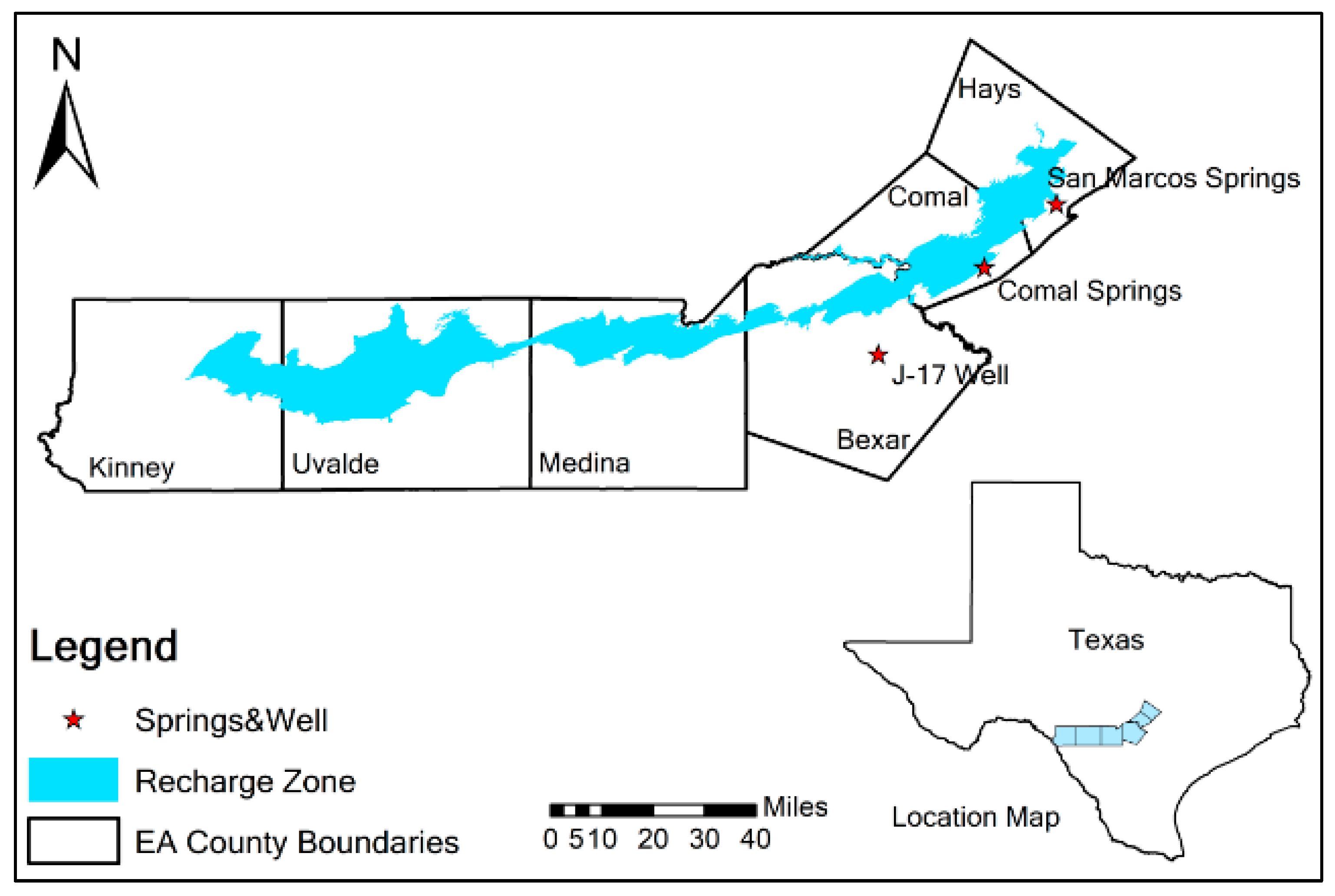
EDSIM depicts the activity in parts of six counties that constitute the recharge and pumping use zone of the EA. The counties are Kinney, Uvalde, Medina, Bexar, Comal, and Hays. Study area is shown in Figure 1. Data are generally at the county level. When county-level data were unavailable, then district data were used mainly for crop and livestock production budget data. We discussed the basics of the data below with details provided in Ding [44].
5.1. Crop and Livestock Data
Crop budget data were drawn from the annual budgets produced by the Texas A&M AgriLife Extension Service. These budget data include crop yield, price, and input cost with year 2011 being used. Crop mix data were drawn from Quick Stats, National Agricultural Statistics Services (NASS) and the Census of Agriculture. The mix data included the harvested acreage by crop.
The livestock budgets also came from the Texas A&M Agrilife Extension Service although due to data availability we had used information from an adjacent region [45]. The budgets were defined on an animal unit (AU) basis. One head of cattle was treated as one animal unit, and six head of goats and five head of sheep were also considered on one animal unit [46]. The net benefit per AU was specified as the returns above direct expenses less the cost of grassland use per acre per AU. Livestock mix were defined based on inventory which were collected from Quick Stats, NASS.
5.2. Recharge Data and States of Nature
Following the original EDSIM, there are nine recharge states that range from heavily dry to heavily wet based on regional US geological survey data as reported by the EAA. To form these, we clustered the historical annual recharge data into the nine states of nature. Table 2 shows the recharge states and the corresponding typical weather years clustered into each. The probability of a recharge state was defined as the relative incidence of a weather years falling into that state thus, since 3 years fell into the ‘heavily dry’ category, we used 3 divided by 78 as the probability. Based on the typical weather years, we obtained the probability distribution of the recharge state (see Table 2). Following Cai [47], the dry years in Table 2 were classified as drought years; normal as normal years, and the remainder as wet years. Hence, the probabilities for drought, normal, and wet years were 0.1923, 0.4615, and 0.3462, respectively. In the scenario of increased drought frequency, the summed probability of drought years increased from 0.1923 to 0.3923 by essentially doubling those probabilities and the summed probability of wet years were decreased from 0.3462 to 0.1362. The probability of normal years was not changed. The drought frequency is simply defined as the summed probability of drought years without considering the temporal or seasonal nature of droughts.
5.3. Land Availability
Land availability data were obtained from the 2007 Census of Agriculture. Cropland was categorized as irrigated land and dryland, and irrigated land was further classified as furrow and sprinkler land. Three pumping lift zones were considered here to reflect initial depth to water. The availability of sprinkler land in each lift zone was calculated based on the zonal percentage of total pumping use, and then the available furrow land in each zone was the difference between the irrigated land in each zone and the estimated sprinkler land. As in McCarl et al. [32], dryland was initially set as zero because we focused on studying land use and conversion.
Grassland use was added to the EDSIM. We assumed that all of the grassland is non-irrigated [45]. Furrow or sprinkler land can be converted to dryland or grassland.
5.4. Municipal and Industrial Water Usage
Water usage data in the M&I sectors were based on the Hydrologic Data Report from the EAA website [48]. The water usage data were annual, although we needed monthly data for the EDSIM. Therefore, the 2011 monthly M&I water usage data were calculated based on the monthly distribution of water use in 1996. The elasticity of municipal demand was from Griffin and Chang [49], while the elasticity of industrial demand came from Renzetti [50].
5.5. Linkages between Water Usage, Spring Flows, and Aquifer Elevation
A critical part of the study involved linking the spring flow and aquifer elevation to water usage. This was done using functions estimated by Keplinger and McCarl [51] that related spring flow and ending elevation levels to the initial water level, pumping, and recharge level by states of nature.
6. Model Results and Discussion
In doing our analysis, we first solved the model with and without increasing the drought frequency and reported the results on welfare, land use, water use, springflow, and ending elevation under various scenarios. Later we examined how welfare changes under different degrees of increased drought incidence.
6.1. Welfare Effects
Table 3 presents the welfare effects with and without increased drought frequency. First, we considered the base results for no changes in drought probability. Under 2011 conditions, the crop income is $211.75 million and livestock income is $54.80 million. When a 400 thousand acre-feet limit (2011Base400) is considered, the results show a crop income reduction of $8.24 million per year, which is 3.89% below the baseline income level. Income from livestock production increases by $2.38 million, which is 4.34% of the base year income. This reflects land moving out of irrigation and into grassland. The loss in M&I surplus is less than 0.1% of the baseline surplus. The percentage change in M&I surplus is small because the water demand curve in these two sectors is fairly inelastic with water values being substantially higher.
If the pumping limit is stricter, e.g., 375 thousand acre-feet, then the welfare changes in each sector are larger. Compared with the effects under pumping limits of 400 thousand acre-feet and 375 thousand acre-feet, the effects of a springflow limit of 225 cfs on welfare are smaller because the total water use under this limit is greater than 400 thousand acre-feet (see Table 5). The springflow limit is not as strict in limiting the water use in the EA region because the springflow limit allows more water use in wet years and in fact is the way that the aquifer is managed currently.
Moreover, if the M&I water demand increases by 10%, which is observed in the 10Base400, 10Base375 and 10Base+Spring225 scenarios, crop income shows greater decreases while livestock income increases slightly; however, the M&I surplus increases greatly because the water demand curves for these sectors shift outward.
A drought probability increase of 0.2 yields more extreme results. If a pumping limit is not considered, then increased drought will lead to a cropping loss of $6.88 million and a total surplus loss of $2.40 million with water flowing to M&I interests. These losses are larger under pumping limits, and they also significantly reduce springflow, which will be shown in a later hydrologic section. Under a 400 thousand acre-feet pumping limit, additional frequent droughts will cause a greater cropping loss of $6.14 million. Income from the livestock sector decreases slightly, whereas the M&I surplus increases because water flows to more valued users. Increased drought also results in a total welfare loss of $1.75 million per year. When stricter pumping limits are imposed, cropping losses due to more frequent droughts are lower. For example, under 375 thousand acre-feet pumping limit (2011Base375), increased drought will cause cropping losses of $5.98 million, whereas additional frequent droughts under 400 thousand acre-feet pumping limit will cause crop losses of $6.14 million.
As water demand in the M&I sectors increases and lower pumping limits are imposed, then cropping income declines more and livestock income increases. If the M&I water demand increases by 10%, more frequent drought will increase the competition for water allocation among irrigation, municipal, and industrial users. Additional water flows to the M&I sectors leads to more losses in cropping income. For example, under a minimum springflow of 225 cfs (10Base+Spring225), increased drought causes a cropping loss of $8.42 million per year and livestock income increase of $0.68 million per year.
6.2. Land Use
Data in Table 4 portray land use impacts with and without altered drought frequency. There is no irrigated land converted to grassland when no pumping limits are imposed. For cases of no changes in drought incidence, the lower pumping limit of 400 thousand acre-feet results in land conversion of 10.54 thousand acres from furrow land to grassland and 20.65 thousand acres from sprinkler land to grassland. When much stricter pumping limits are imposed (2011Base375), more furrow land and sprinkler land are converted to grassland. The impact from imposing a minimum springflow constraint is smaller than that from a pumping limit for the same reason provided above. The impacts on land use will be greater if there is an increase in M&I water demand of 10%.
When the drought probability increases by 0.2 under the 2011Base400 scenario, the conversion of furrow land to grassland becomes 0 acres, whereas additional frequent droughts causes more conversion of 11.52 thousand acres from sprinkler land to grassland. Increased land conversion of sprinkler land to grassland also occurs under the other scenarios. For instance, under the scenario of 2011Base375, more frequent droughts reduce the sprinkler land by 16.48 thousand acres via the conversion to grassland. Furthermore, the drought impact on land use change increases in severity when the M&I water demand increases by 10%, which also increases the conversion of irrigated land to grassland. For example, a comparison of scenarios 10Base400 with and without increasing drought frequency shows that when drought becomes more frequent, additional sprinkler land is converted to grassland while less furrow land is converted to grassland. Land transfers increase when water allocation becomes more competitive, i.e., under a pumping limit of 375 thousand acre-feet.
6.3. Water Use
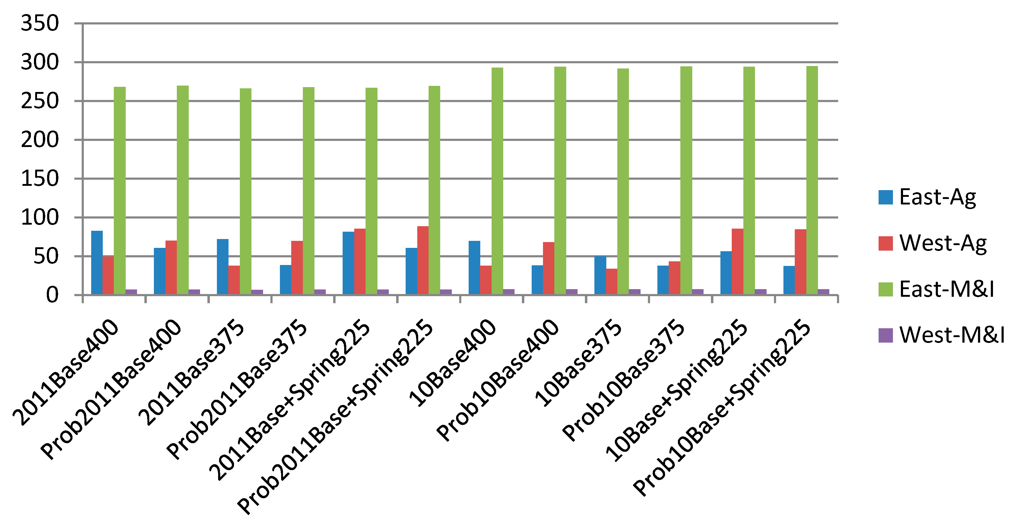
Table 5 shows water use with and without increases in drought frequency. When droughts do not increase and the total water withdrawn from the aquifer is restricted to 400 thousand acre-feet, then the total water usage is reduced by 102.17 thousand acre-feet, with 89.88% of the reduction from agriculture, primarily in the east region (see Figure 2). When springflow is limited to be greater than 225 cfs, east agricultural water use also decreases considerably. A 10% increase in M&I water demand further reduces the water usage by agriculture.
Now, we consider the effect of increased drought on water use. When the total water pumping is limited to 400 thousand acre-feet, more frequent droughts will cause a further reduction of agricultural water use of 2,160 acre-feet and a total water usage decrease of 560 acre-feet. If the total water pumped from the aquifer is restricted to 375 thousand acre-feet, then agricultural water use further declines by 1,480 acre-feet and the total water usage is reduced by 100 acre-feet. However, when springflow limit of 225 cfs is imposed, more frequent droughts will cause more reduction in agricultural water use. The above comparison indicates that stricter pumping constraints lower the impact of increased drought on water allocation because ample water is frequently observed. Furthermore, drought impacts on irrigation water use increase if the M&I water demand increases by 10%, with the impacts mainly on eastern region irrigation water use (see Figure 2).
6.4. Hydrologic Impacts
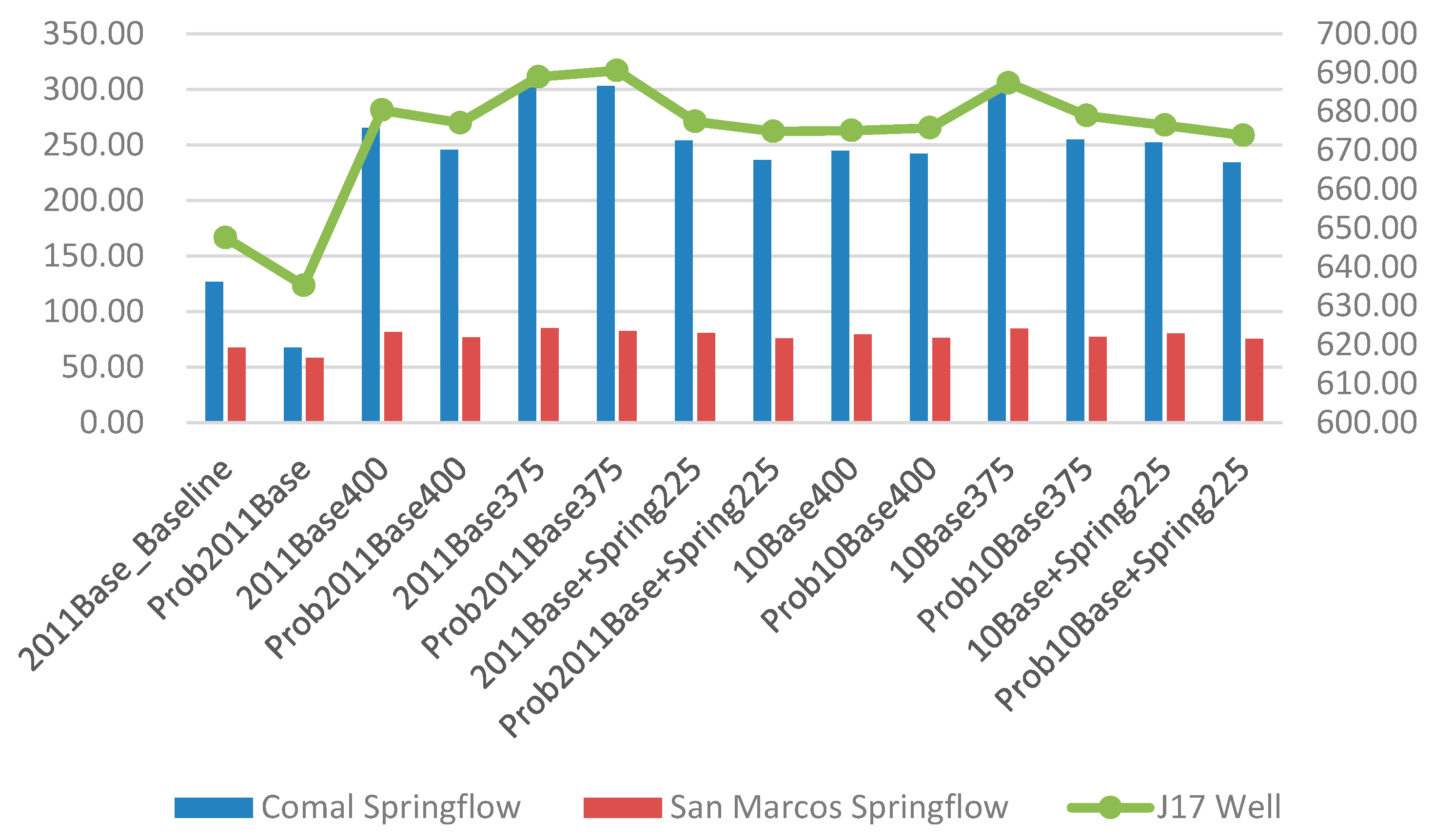
Figure 3 presents a comparison of the hydrologic impacts. When the drought probability is not changed, both the pumping and minimum springflow limits increase the springflow in both Comal Spring and San Marcos Spring, and the J17 well water elevation as well. The lower pumping limit (375 thousand acre-feet) increases the springflow and the J17 well water elevation the most. If the M&I water demand keeps unchanged, the 400 pumping limit protects the springflow and well elevation better than does the springflow restriction. However, when the M&I water demand goes up by 10%, the role of springflow restriction is bigger than 400 pumping limit.
When the drought probability increases by 0.2, the springflow and the J17 well elevation are reduced. If there are no restrictions on pumping or springflow, increased drought will cause the springflow and J17 well end elevation decline greatly, which further emphasizes the importance of pumping limits and/or minimum springflow limits. Again, the impacts are smaller with a pumping restriction of 375 thousand acre-feet because this limit provide a safety margin. Similar results are observed when the M&I water demand increases. Note here in the case if both the M&I water demand and drought frequency increase, pumping limits can help better protect springflow and well elevation than springflow restriction, probably because pumping limits can overall plan the use of water resources when water use competition is stricter.
6.5. Comparison of the Impacts under Different Changes in Drought Probability
Table 6 reports the impacts under different changes in drought frequency. Here we consider drought probability increase from 0.1 to 0.3, which holds the probability of normal years unchanged and let the drought probability increase and the wet probability decrease in the relative amount. According to Zhao et al. [52], they projected that the probability distribution function (pdf) of agricultural drought would become flatter. We also consider a scenario that drought probability increases 0.2 and normal year probability and wet probability decreases 0.1, respectively. The first four lines of Table 6 present the average economic benefit under different degrees of drought frequency change. The baseline presents the case when the total water pumped is limited to 400 thousand acre-feet. In turn, if the probability of drought increases by 0.1, then cropping will suffer a loss of $2.97 million. Moreover, the income from livestock production will decrease slightly, the M&I surplus will increase by $2.13 million, and increased drought will cause a total surplus loss of $1.03 million per year.
When droughts become more frequent, the cropping loss will be greater and the acreage of irrigated land will decrease. When the drought probability increases by 0.1, additional irrigated farming is conducted; however, as droughts become more frequent, irrigated acreage decreases and more land is converted to grassland. When grassland acreage increases, livestock income increases as well. In terms of water use and hydrologic impact, water reductions primarily occur in the irrigation use. Additionally, as droughts become more frequent, the springflow in both of the springs and the J17 well water elevation are reduced. More frequent droughts reduce the springflow, and stricter pumping limits or springflow restrictions would be required to maintain current springflow levels and protect spring-supported endangered species.
7. Conclusions
EA recharge mainly relies on rainfall, which would be negatively affected by the increased incidence of drought proved by a number of studies in the IPCC [2]. In particular, drought frequency is predicted to increase in the southwestern U.S., where the EA is located [17,18]. We find that such developments would shift water from cropping to M&I interests with decreases in cropping income, increases in livestock income and not much effect on the M&I welfare. We find that under a pumping limit of 400 thousand acre-feet, an increased drought frequency will result in a regional cropping loss of $6.14 million per year, with yet more water reallocated to M&I interests. Stricter pumping limitations, such as a 375 thousand acre-feet pumping limit, help alleviate the cropping losses under the increased drought scenario principally due to lower pump lifts.
We also found that more frequent droughts will increase land transfers from irrigated land to grassland and livestock uses, while decreasing springflows in both Comal Spring and San Marcos Spring. To preserve the endangered species habitat surrounding the springs, lower maximum pumping limits or minimum springflow restrictions are required. There are also ecological implications of this in that there are several endangered species whose habitat is supplied by the springflow plus a change from irrigated agriculture to grassland-based livestock would certainly bring about a number of other ecological alterations.
Author Contributions
Conceptualization, B.A.M.; methodology, B.A.M. and J.D.; software, J.D.; validation, J.D.; formal analysis, J.D.; investigation, J.D.; resources, B.A.M. and J.D.; data curation, J.D.; writing—original draft preparation, J.D.; writing—review and editing, B.A.M. and J.D.; visualization, J.D.; supervision, B.A.M.; project administration, J.D.; funding acquisition, B.A.M. and J.D. All authors have read and agreed to the published version of the manuscript.
Funding
This research was partially funded by the NOAA—Climate Programs Office—Sectoral Applications Research Program under grant NA12OAR4310097 and the U.S. Department of Agriculture—National Institute of Food and Agriculture under grant 2011-67003-30213 in the NSF—USDA—DOE Earth System Modelling Program. In addition while the majority of this work was done at Texas A&M University, some was also done at Xiamen University with funding provided by the Chinese Fundamental Research Funds for the Central Universities under grant 20720151281. We acknowledge the support of both institutions.
Acknowledgments
We thank David Anderson and Chengcheng Fei at Texas A&M University for their helpful comments. Two anonymous referees provided comments that improved the initial version of this paper.
Conflicts of Interest
The authors declare no conflict of interest.
Appendix A. EDSIM Model Concept and Structure
Before presenting the fundamental algebraic structure of the EDSIM, we will overview its theoretical structure. In brief, EDSIM is a price endogenous mathematical program that can be represented by the following Equation (A1),
where and are the quantities demanded and supplied, respectively; is the inverse demand curve that provides the demand price as a function of the quantity demanded; and is the inverse supply curve that provides the supply price as a function of the quantity supplied. The objective function is the sum of the consumers’ plus producers’ surplus in the EA region subject to hydrological, land, and institutional constraints. The model is stochastic facing nine states of nature where the model must make certain choices (crop mix, livestock herd size, land transformation) before knowing the state of nature and then others dependent on the state of nature (irrigation strategy, crop harvest and sale, livestock sale, municipal and industrial water consumption). The first-order conditions of such a model render the model solution as a simulation of what would happen under a perfectly competitive regional allocation of resources [41,42].
Appendix A.1. Objective Function
The objective function depicts the expected consumers’ plus producers’ surpluses. In this case due to the extremely small share of US production in the region fixed prices are used for agricultural commodities. Consequently, the objective function maximizes the revenue from crop and livestock production plus the area under the M&I demand curves less the costs of crop production, livestock production, and development of irrigated land and costs of lift-dependent pumping. Also, stochastics are present with some terms independent of state of nature and other terms dependent. More precisely, the objective function is presented as follows, with variables in upper case and parameters in lower case.
The first part (first line) of Equation (A2) contains two costs and is independent of state of nature. One is the unit cost of irrigation development (irrcost) by lift zone (z) multiplied by the irrigated land developed (IRRLAND), the other is the cost of converting furrow land to sprinkler land (FURRTOSPK) in a county (p) and lift zone (z).
The second part of Equation (A2) in brackets is stochastic based on the recharge state (r) and is weighted by the probability (prob) of each state. The first two lines depict the net revenue from crop yields, which is the crop revenue minus production costs per acre (irrincome and dryincome) multiplied by the acres produced (IRRPROD and DRYPROD) summed across each county (p), pumping zone (z), crop (c), recharge state (r), and irrigation strategy (s). The third line subtracts irrigation water pumping cost (the variable AGPUMPCOST) multiplied by water use (AGWATER) by county (p) and lift zone (z) in month (m) under recharge state (r). Lines 4 and 5 represent livestock production net revenue, which includes the livestock net income (liveincome) multiplied by livestock raised (LIVEPROD) by livestock type (l), county (p) and lift zone (z) under the recharge state (r). We also deducted the cost of grassland maintenance (grasscost) times the grassland used (GRASSUSE) by county (p) and lift zone (z) and recharge state (r). The last three lines represent the M&I benefits and costs of water pumping, which involves the area under the M&I demand curves less pumping cost (a variable MIPUMPCOST) by county (p) under recharge state (r). The variables MUN and IND represent the amount of water demanded in the M&I sectors, respectively.
Appendix A.2. Land Availability Constraint
Equation (A3) limits irrigated land use by crop (c) and irrigation strategy (s) in a lift zone (z) and county (p) under recharge state (r) (IRRPROD) to the total irrigated land (IRRLAND). The total irrigated land does not vary by recharge state, meaning that it is set before climate conditions are known, however, the irrigated land choice is in a recharge state dependent on the crop use and irrigation strategy.
The initial availability of dryland is zero because we only examine initially irrigated land area. Equation (A4) requires that dryland use in a county (DRYPROD) does not exceed the land converted from irrigated land to dryland (IRRTODRY) by county and lift zone. Note that the dryland available through conversion is the same across all recharge states, but the dryland use can vary by recharge state.
Equation (A5) balances the total initial irrigated land where land used in irrigated cropping (IRRLAND) plus the amount converted to dryland (IRRTODRY) or grassland (IRRTOGRS) cannot exceed the initial availability (irrlandavail) in a county and lift zone. Note that the available converted land is the same across all recharge states.
Equation (A6) is the grassland availability constraint, which limits grassland use (GRASSUSE) to the initial grassland availability (grasslandavail) plus land transformed from irrigated land to grassland (IRRTOGRS) by county (p) and lift zone (z). Note that the available grassland is the same across all recharge states but the grassland use can vary by recharge state. Equation (A7) restricts livestock production and grassland use by county (p) and lift zone (z) under recharge state (r), where gr denotes the grazing rate, which is the amount of grassland required per animal unit.
Appendix A.3. Crop Mix Constraint
Following McCarl (1982), the crop mix restriction requires that crop production is a convex combination of historical crop mixes, which is performed for irrigated land and dryland separately. Thus, irrigated land produced (IRRPROD) is a convex combination of historical irrigated crop mixes (irrmixdata) in terms of crops (c) and mix possibilities (x) in county (p) in Equation (A8). Similarly, dryland produced (DRYPROD) is a convex combination of historical dryland crop mixes (drymixdata) in Equation (A9). The separate limits for irrigated land and dryland allow their acreage to vary independently as more or less land is converted. A separate mix is allowed for each lift zone causing realistic crop mixes on each zone. The crop mix approach is used to make realistic crop mixes without modeling detailed resource allocation at the farm level [53].
Appendix A.4. Livestock Mix Restriction
Livestock mixes are also defined in Equation (A10). Livestock production (LIVEPROD) by livestock type for a county and zone under a recharge state is set to be a convex combination of historical observable livestock mixes (livemixdata) in terms of species. As argued by McCarl [53], this constraint can make realistic livestock mixes without modeling the detailed resource allocation at the farm level.
Appendix A.5. Lift Dependent Pumping Cost
Equations (A11) and (A12) relate the pumping cost to aquifer lift which is determined by the next equation. The agricultural pumping cost per acre-foot of water for county, zone, and recharge state equals a fixed pumping cost (agcpump) plus a variable pumping cost (agvpump) per foot of lift multiplied by the agricultural lift (AGLIFT). Similarly, the M&I pumping costs per acre-foot are similarly defined.
Appendix A.6. Aquifer Elevation Determination
The ending water elevation level of the EA is calculated via Equation (A13), which relates the ending water level to a regression-estimated function that was developed by Keplinger and McCarl [51]. Namely we determine elevation as a function of monthly recharge level (rech), initial water level (INITWATER), and total water use. Total water usage is the sum of municipal (MUN), industrial (IND), and agricultural (AGWATER) water use.
In Equation (A13), rendint is the estimated intercept, rendr is the parameter of recharge, rende is the initial water parameter, and rendu is the parameter of total water use. The subscript w refers to the region where the elevation is calculated, and the subscript w2 is used to sum the water use across both the east and the west EA regions.
Appendix A.7. Springflow Equation
Springflow levels are defined in Equation (A14), which relates springflow level to a regression-estimated function again from Keplinger and McCarl [51]. That function relates monthly springflow by spring s to monthly recharge in previous part of year, initial water level, and total water use. Therein rsprnint is the estimated intercept, rsprnr is the parameter of recharge, rsprne is the initial water parameter, and rsprnu is the parameter of total water use. Both subscripts m and m* refer to the month.
References
- EAA. 2018 Groundwater Discharge and Usage. Available online: https://www.edwardsaquifer.org/wp-content/uploads/2019/08/2018-Discharge-Report.pdf (accessed on 19 December 2019).
- IPCC. Managing the Risks of Extreme Events and Disasters to Advance Climate Change Adaptation. In A Special Report of Working Groups I and II of the Intergovernmental Panel on Climate Change; Field, C.B., Barros, V., Stocker, T.F., Qin, D., Dokken, D.J., Ebi, K.L., Mastrandrea, M.D., Mach, K.J., Plattner, G.-K., Allen, S.K., et al., Eds.; Cambridge University Press: Cambridge, UK; New York, NY, USA, 2012; pp. 25–231. [Google Scholar]
- Schwalm, C.R.; Anderegg, W.R.L.; Michalak, A.M.; Fisher, J.B.; Biondi, F.; Koch, G.; Litvak, M.; Ogle, K.; Shaw, J.D.; Wolf, A.; et al. Global Patterns of Drought Recovery. Nature 2017, 548, 202–205. [Google Scholar] [CrossRef] [PubMed]
- Spinoni, J.; Vogt, J.V.; Naumann, G.; Barbosa, P.; Dosio, A. Will Drought Events Become More Frequent and Severe in Europe? Int. J. Climatol. 2018, 38, 1718–1736. [Google Scholar] [CrossRef] [Green Version]
- Touma, D.; Ashfaq, M.; Nayak, M.A.; Kao, S.C.; Diffenbaugh, N.S. A Multi-model and Multi-index Evaluation of Drought Characteristics in the 21st Century. J. Hydrol. 2015, 526, 196–207. [Google Scholar] [CrossRef] [Green Version]
- Yuan, X.; Zhang, M.; Wang, L.; Zhou, T. Understanding and Seasonal Forecasting of Hydrological Drought in the Anthropocene. Hydrol. Earth Syst. Sci. 2017, 21, 5477–5492. [Google Scholar] [CrossRef] [Green Version]
- IPCC. Climate Change 2014: Impacts, Adaptation, and Vulnerability. Part A: Global and Sectoral Aspects. In Contribution of Working Group II to the Fifth Assessment Report of the Intergovernmental Panel on Climate Change; Field, C.B., Barros, V.R., Dokken, D.J., Mach, K.J., Mastrandrea, M.D., Bilir, T.E., Chatterjee, M., Ebi, K.L., Estrada, Y.O., Genova, R.C., et al., Eds.; Cambridge University Press: Cambridge, UK; New York, NY, USA, 2014; pp. 229–269. [Google Scholar]
- Aryal, Y.; Zhu, J. On Bias Correction in Drought Frequency Analysis Based on Climate Models. Clim. Chang. 2017, 140, 361–374. [Google Scholar] [CrossRef]
- Sheffield, J.; Wood, E.F. Projected Changes in Drought Occurrence under Future Global Warming from Multi-model, Multi-scenario, IPCC AR4 Simulations. Clim. Dyn. 2008, 31, 79–105. [Google Scholar] [CrossRef]
- Trenberth, K.E.; Fasullo, J.T. An Apparent Hiatus in Global Warming? Earths Future 2013, 1, 19–32. [Google Scholar] [CrossRef]
- Bastos, A.; Running, S.W.; Gouveia, C.; Trigo, R.M. The Global NPP Dependence on ENSO: La Niña and the Extraordinary Year of 2011. J. Geophys. Res. Biogeosci. 2013, 118, 1247–1255. [Google Scholar] [CrossRef] [Green Version]
- Chen, C.C.; Gillig, D.; McCarl, B.A.; Williams, R.L. ENSO Impacts on Regional Water Management: Case Study of the Edwards Aquifer (Texas, USA). Clim. Res. 2005, 28, 175–182. [Google Scholar] [CrossRef] [Green Version]
- Long, D.; Scanlon, B.R.; Longuevergne, L.; Sun, A.Y.; Fernando, D.N.; Save, H. GRACE Satellite Monitoring of Large Depletion in Water Storage in Response to the 2011 Drought in Texas. Geophys. Res. Lett. 2013, 40, 3395–3401. [Google Scholar] [CrossRef] [Green Version]
- Gulley, R.L.; Cantwell, J.B. The Edwards Aquifer Water Wars: The Final Chapter? Tex. Water J. 2013, 4, 1–21. [Google Scholar]
- Edwards Aquifer Habitat Conservation Plan 2018 Annual Report. Available online: https://www.edwardsaquifer.org/wp-content/uploads/2019/10/EAHCP_Annual_Report_2018.pdf (accessed on 19 December 2019).
- Uddameri, V.; Singaraju, S.; Hernandez, E.A. Is Standardized Precipitation Index (SPI) a Useful Indicator to Forecast Groundwater Droughts?—Insights from a Karst Aquifer. J. Am. Water Resour. Assoc. 2019, 55, 70–88. [Google Scholar] [CrossRef]
- Seager, R.; Ting, M.; Held, I.; Kushnir, Y.; Lu, J.; Vecchi, G.; Huang, H.P.; Harnik, N.; Leetmaa, A.; Lau, N.C.; et al. Model Projections of an Imminent Transition to a More Arid Climate in Southwestern North America. Science 2007, 316, 1181–1184. [Google Scholar] [CrossRef] [PubMed]
- Cayan, D.R.; Das, T.; Pierce, D.W.; Barnett, T.P.; Tyree, M.; Gershunov, A. Future Dryness in the Southwest US and the Hydrology of the Early 21st Century Drought. Proc. Natl. Acad. Sci. USA 2010, 107, 21271–21276. [Google Scholar] [CrossRef] [PubMed] [Green Version]
- IPCC. Climate Change 2007: The Physical Science Basis. In Contribution of Working Group I to the Fourth Assessment Report of the Intergovernmental Panel on Climate Change; Solomon, S., Qin, D., Manning, M., Chen, Z., Marquis, M., Averyt, K.B., Tignor, M., Miller, H.L., Eds.; Cambridge University Press: Cambridge, UK, 2007; pp. 847–940. [Google Scholar]
- Diffenbaugh, N.S.; Swain, D.L.; Touma, D. Anthropogenic Warming Has Increased Drought Risk in California. Proc. Natl. Acad. Sci. USA 2015, 112, 3931–3936. [Google Scholar] [CrossRef] [PubMed] [Green Version]
- Bazargan-Lari, M.R.; Kerachian, R.; Mansoori, A. A Conflict-resolution Model for the Conjunctive Use of Surface and Groundwater Resources that Considers Water-quality Issues: A Case Study. Environ. Manag. 2009, 43, 470. [Google Scholar] [CrossRef]
- Li, Z.; Quan, J.; Li, X.Y.; Wu, X.C.; Wu, H.W.; Li, Y.T.; Li, G.Y. Establishing a Model of Conjunctive Regulation of Surface Water and Groundwater in the Arid Regions. Agric. Water Manag. 2016, 174, 30–38. [Google Scholar] [CrossRef]
- Daneshmand, F.; Karimi, A.; Nikoo, M.R.; Bazargan-Lari, M.R.; Adamowski, J. Mitigating Socio-economic-environmental Impacts during Drought Periods by Optimizing the Conjunctive Management of Water Resources. Water Resour. Manag. 2014, 28, 1517–1529. [Google Scholar] [CrossRef]
- Pulido-Velazquez, M.; Jenkins, M.W.; Lund, J.R. Economic Values for Conjunctive Use and Water Banking in Southern California. Water Resour. Res. 2004, 40. [Google Scholar] [CrossRef] [Green Version]
- Castaño, S.; Sanz, D.; Gómez-Alday, J.J. Sensitivity of a Groundwater Flow Model to Both Climatic Variations and Management Scenarios in a Semi-arid Region of SE Spain. Water Resour. Manag. 2013, 27, 2089–2101. [Google Scholar] [CrossRef]
- Golden, B.; Johnson, J. Potential Economic Impacts of Water-use Changes in Southwest Kansas. J. Natl. Resour. Policy Res. 2013, 5, 129–145. [Google Scholar] [CrossRef]
- Dai, Z.; Du, J.; Chu, A.; Li, J.; Chen, J.; Zhang, X. Groundwater Discharge to the Changjiang River, China, during the Drought Season of 2006: Effects of the Extreme Drought and the Impoundment of the Three Gorges Dam. Hydrogeol. J. 2010, 18, 359–369. [Google Scholar] [CrossRef]
- Calow, R.C.; Robins, N.S.; Macdonald, A.M.; Macdonald, D.M.J.; Gibbs, B.R.; Orpen, W.R.G.; Mtembezeka, P.; Andrews, A.J.; Appiah, S.O. Groundwater Management in Drought-prone Areas of Africa. Int. J. Water Resour. Dev. 1997, 13, 241–261. [Google Scholar] [CrossRef]
- Shahid, S.; Hazarika, M.K. Groundwater Drought in the Northwestern Districts of Bangladesh. Water Resour. Manag. 2010, 24, 1989–2006. [Google Scholar] [CrossRef]
- Scanlon, B.R.; Mace, R.E.; Barrett, M.E.; Smith, B. Can We Simulate Regional Groundwater Flow in a Karst System Using Equivalent Porous Media Models? Case Study, Barton Springs Edwards aquifer, USA. J. Hydrol. 2003, 276, 137–158. [Google Scholar] [CrossRef]
- Loaiciga, H.A.; Maidment, D.R.; Valdes, J.B. Climate-change Impacts in a Regional Karst Aquifer, Texas, USA. J. Hydrol. 2000, 227, 173–194. [Google Scholar] [CrossRef]
- McCarl, B.A.; Dillon, C.R.; Keplinger, K.O.; Williams, R.L. Limiting Pumping from the Edwards Aquifer: An Economic Investigation of Proposals, Water Markets, and Spring Flow Guarantees. Water Resour. Res. 1999, 35, 1257–1268. [Google Scholar] [CrossRef]
- Chen, C.; Gillig, D.; McCarl, B.A. Effects of Climatic Change on A Water Dependent Regional Economy: A study of the Texas Edwards Aquifer. Clim. Chang. 2001, 49, 397–409. [Google Scholar] [CrossRef]
- Gillig, D.; McCarl, B.A.; Boadu, F. An Economic, Hydrologic, and Environmental Assessment of Water Management Alternative Plans for the South Central Texas Region. J. Agric. Appl. Econ. 2001, 33, 59–78. [Google Scholar] [CrossRef] [Green Version]
- Chen, C.; McCarl, B.A.; Williams, R.L. Elevation Dependent Management of the Edwards Aquifer: Linked Mathematical and Dynamic Programming Approach. J. Water Resour. Plan. Manag. 2006, 132, 330–340. [Google Scholar] [CrossRef]
- Gray, E.; Henninger, N.; Reij, C.; Winterbottom, R.; Agostini, P. Integrated Landscape Approaches for Africa’s Drylands; The World Bank: Washington, DC, USA, 2016; pp. 61–129. [Google Scholar]
- Alary, V.; Messad, S.; Aboul-Naga, A.; Osman, M.A.; Daoud, I.; Bonnet, P.; Juanes, X.; Tourrand, J.F. Livelihood Strategies and the Role of Livestock in the Processes of Adaptation to Drought in the Coastal Zone of Western Desert (Egypt). Agric. Syst. 2014, 128, 44–54. [Google Scholar] [CrossRef]
- Adamson, D.; Mallawaarachchi, T.; Quiggin, J. Declining Inflows and More Frequent Droughts in the Murray Darling Basin: Climate Change, Impacts and Adaptation. Aust. J. Agric. Resour. Econ. 2009, 53, 345–366. [Google Scholar] [CrossRef]
- Cañón, J.; González, J.; Valdés, J. Reservoir Operation and Water Allocation to Mitigate Drought Effects in Crops: A Multilevel Optimization Using the Drought Frequency Index. J. Water Resour. Plan. Manag. 2009, 135, 458–465. [Google Scholar] [CrossRef]
- Ward, F.A.; Hurd, B.H.; Rahmani, T.; Gollehon, N. Economic Impacts of Federal Policy Responses to Drought in the Rio Grande Basin. Water Resour. Res. 2006, 42. [Google Scholar] [CrossRef] [Green Version]
- McCarl, B.A.; Spreen, T.H. Price Endogenous Mathematical Programming as a Tool for Sector Analysis. Am. J. Agric. Econ. 1980, 62, 87–102. [Google Scholar] [CrossRef] [Green Version]
- Lambert, D.K.; McCarl, B.A.; He, Q.; Kaylen, M.S.; Rosenthal, W.; Chang, C.C.; Nayda, W.I. Uncertain Yields in Sectoral Welfare Analysis: An Application to Global Warming. J. Agric. Appl. Econ. 1995, 27, 423–436. [Google Scholar] [CrossRef] [Green Version]
- Dantzig, G.B. Linear Programming under Uncertainty. Manag. Sci. 1995, 1, 197–206. [Google Scholar] [CrossRef]
- Ding, J. Three Essays on Climate Variability, Water and Agricultural Production. Ph.D. Thesis, Texas A&M University, College Station, TX, USA, 2014. [Google Scholar]
- Anderson, D.; (Texas A&M University: College Station, TX, USA). Personal communication, 2014.
- Lyons, R.K.; Machen, R.V. Stocking Rate: The Key Grazing Management Decision. Texas FARMER Collection 2004. Available online: https://core.ac.uk/download/pdf/4274892.pdf (accessed on 8 November 2019).
- Cai, Y. Water Scarcity, Climate Change, and Water Quality: Three Economic Essays. Ph.D. Thesis, Texas A&M University, College Station, TX, USA, 2009. [Google Scholar]
- Hydrologic Data Report. Available online: https://www.edwardsaquifer.org/science-maps/research-scientific-reports/hydrologic-data-reports/ (accessed on 19 December 2019).
- Griffin, R.C.; Chang, C. Seasonality in Community Water Demand. West. J. Agric. Econ. 1991, 16, 207–217. [Google Scholar]
- Renzetti, S. An Economic Study of Industrial Water Demands in British Columbia, Canada. Water Resour. Res. 1988, 24, 1569–1573. [Google Scholar] [CrossRef]
- Keplinger, K.O.; McCarl, B.A. The Effects of Recharge, Agricultural Pumping and Municipal Pumping on Springflow and Pumping Lifts Within the Edwards Aquifer: A Comparative Analysis Using Three Approaches; Texas A&M University: College Station, TX, USA, 1995; Available online: http://agecon2.tamu.edu/people/faculty/mccarl-bruce/papers/584.pdf (accessed on 8 November 2019).
- Zhao, T.; Dai, A. Uncertainties in Historical Changes and Future Projections of Drought. Part II: Model-simulated Historical and Future Drought Changes. Clim. Chang. 2017, 144, 535–548. [Google Scholar] [CrossRef]
- McCarl, B.A. Cropping Activities in Agricultural Sector Models: A Methodological Proposal. Am. J. Agric. Econ. 1982, 64, 768–772. [Google Scholar] [CrossRef]
Figure 1.
Edwards aquifer region and typical springs and well.

Figure 2.
Water use in the east and west region in the agricultural and M&I sectors. Note: (1) Definitions of scenarios are provided in Table 1. (2) When the drought frequency is increased by 0.2, each scenario is prefixed with “Prob”. (3) East-Ag and West-Ag represent the water use of agriculture in east and west EA regions, respectively, and East-M&I and West-M&I are the municipal and industrial water use in the east and west EA region, respectively.

Figure 3.
Comparison of hydrologic impacts with and without increased drought. Note: (1) Definitions of scenarios are provided in Table 1. (2) When the drought frequency is increased by 0.2, each scenario is prefixed with “Prob”. (3) “Comal Springflow” and “San Marcos Springflow” refer to the springflow in Comal Spring and San Marcos Spring, respectively (103 acre feet). (4) “J17 Well” refers to the elevation of a reference well in San Antonio (feet).


Table 1.
Definition of scenarios.
| Scenarios | Definition |
|---|---|
| 2011Base | Baseline |
| 2011Base400 | Base model with pumping limit of 400 thousand acre-feet |
| 2011Base375 | Base model with pumping limit of 375 thousand acre-feet |
| 2011Base+Spring225 | Base model with minimum springflow of 225 cfs |
| 10Base400 | M&I water demand increases of 10% and 400 thousand acre-feet pumping limit |
| 10Base375 | M&I water demand increases of 10% and 375 thousand acre-feet pumping limit |
| 10Base+Spring225 | M&I water demand increases of 10% and minimum springflow of 225 cfs |
Table 2.
Recharge states, years represented, recharge level, and probability distribution.
| Recharge State | Years (1934-2011) | Recharge Level | Probability |
|---|---|---|---|
| (Typical Weather Years in Bold) | (103 acre-feet) | ||
| Heavily dry | 1956, 2011, 1951 | 43.7 | 0.0385 |
| Medium dry | 1954, 1953, 1963, 1948, 1934 | 170.7 | 0.0641 |
| Dry | 1955, 1984, 1950, 2006, 2008, 2009, 1989 | 214.4 | 0.0897 |
| Dry-normal | 1962, 1943, 1952, 1940 | 275.5 | 0.0513 |
| Normal | 1996, 1988, 1939, 1937, 1980, 1964, 1983, 1982, 1947, 1938, 1993, 1967, 1999, 1978, 1949 | 324.3 | 0.1923 |
| Normal-wet | 1945, 1995, 1994, 1946, 1942, 1944, 1969, 2000, 1966, 1965, 1974, 1970, 2003, 1959, 1961, 2005, 1972 | 658.5 | 0.2179 |
| Wet | 2010, 1960, 1941, 1968, 1976, 1936, 1971, 1977, 1975, 1985, 2001, 1979, 1990, 1997, 1998, 1957, 1986 | 894.1 | 0.2179 |
| Medium wet | 1935, 1981, 1973, 1991, 2002, 1958 | 1711.2 | 0.0769 |
| Heavily wet | 1987, 2004, 2007, 1992 | 2003.6 | 0.0513 |
| Average | 710.9 |
Table 3.
Comparison of the welfare effect with and without increasing drought frequency.
| Scenarios | Change in Economic Benefit (106$) | ||||
|---|---|---|---|---|---|
| Cropping | Livestock | M&I | Total Surplus | ||
| Prob(Drought) No Change | 2011Base_Baseline | 211.75 | 54.80 | 828.41 | 1094.95 |
| 2011Base400 | −8.24 | 2.38 | −0.64 | −6.50 | |
| 2011Base375 | −11.22 | 3.12 | −0.83 | −8.92 | |
| 2011Base+Spring225 | −4.73 | 1.44 | −0.65 | −3.94 | |
| 10Base400 | −11.47 | 3.20 | 82.04 | 73.72 | |
| 10Base375 | −14.70 | 3.97 | 81.82 | 71.09 | |
| 10Base+Spring225 | −8.13 | 2.24 | 82.20 | 76.31 | |
| Prob(Drought) Increases 0.2 | 2011Base | −6.88 | 0.00 | 4.48 | −2.40 |
| 2011Base400 | −14.38 | 2.35 | 3.79 | −8.25 | |
| 2011Base375 | −17.20 | 3.03 | 3.51 | −10.67 | |
| 2011Base+Spring225 | −13.41 | 2.10 | 3.87 | −7.44 | |
| 10Base400 | −17.45 | 3.09 | 86.78 | 72.43 | |
| 10Base375 | −21.10 | 4.12 | 86.80 | 69.82 | |
| 10Base+Spring225 | −16.55 | 2.92 | 86.98 | 73.35 | |
Note: Definitions of scenarios are provided in Table 1.
Table 4.
Comparison of impacts on land conversion with and without increasing drought frequency.
| Scenarios | Change in Land Use (103acre-feet) | ||
|---|---|---|---|
| FurrowToGrass | SprinklerToGrass | ||
| Prob(Drought) No Change | 2011Base_Baseline | 0.00 | 0.00 |
| 2011Base400 | 10.54 | 20.65 | |
| 2011Base375 | 15.73 | 25.45 | |
| 2011Base+Spring225 | 0.00 | 19.47 | |
| 10Base400 | 15.73 | 26.59 | |
| 10Base375 | 17.80 | 35.27 | |
| 10Base+Spring225 | 0.00 | 30.97 | |
| Prob(Drought) Increases 0.2 | 2011Base | 0.00 | 0.00 |
| 2011Base400 | 0.00 | 32.17 | |
| 2011Base375 | 0.00 | 41.93 | |
| 2011Base+Spring225 | 0.00 | 28.96 | |
| 10Base400 | 0.77 | 42.03 | |
| 10Base375 | 13.76 | 42.03 | |
| 10Base+Spring225 | 0.00 | 40.56 | |
Note: (1) Definitions of scenarios are provided in Table 1. (2) When the drought frequency is increased by 0.2, each scenario is prefixed with “Prob”. (3) FurrowToGrass denotes furrow land converted to grassland. SprinklerToGrass is referred to land conversion from sprinklered land to grassland. There is no land conversion from irrigated land to dryland.
Table 5.
Comparison of the impacts on water use with and without increased drought.
| Scenarios | Change in Water Use (103acre-feet) | |||
|---|---|---|---|---|
| Irrigated Cropping | M&I | Total Value | ||
| Prob(Drought) No Change | 2011Base_Baseline | 224.10 | 284.90 | 509.01 |
| 2011Base400 | −91.83 | −10.34 | −102.17 | |
| 2011Base375 | −114.82 | −12.03 | −126.85 | |
| 2011Base+Spring225 | −57.55 | −11.04 | −68.59 | |
| 10Base400 | −117.06 | 15.21 | −101.85 | |
| 10Base375 | −140.71 | 13.86 | −126.85 | |
| 10Base+Spring225 | −82.90 | 16.36 | −66.55 | |
| Prob(Drought) Increases 0.2 | 2011Base | −0.30 | 1.49 | 1.18 |
| 2011Base400 | −93.99 | −8.74 | −102.73 | |
| 2011Base375 | −116.30 | −10.64 | −126.95 | |
| 2011Base+Spring225 | −74.98 | −8.90 | −83.88 | |
| 10Base400 | −118.14 | 16.51 | −101.63 | |
| 10Base375 | −143.37 | 16.56 | −126.81 | |
| 10Base+Spring225 | −102.36 | 17.41 | −84.95 | |
Note: Definitions of scenarios are provided in Table 1.
Table 6.
Comparison of impacts with various degrees of drought probability change.
| 2011Base400 (Baseline) | Change from Baseline | |||||
|---|---|---|---|---|---|---|
| Prob + 0.1 | Prob +0.2 | Prob + 0.3 | Prob + 0.2 & Flattening pdf | |||
| Economic Benefit(106$) | ||||||
| Cropping | 203.51 | −2.97 | −6.14 | −9.24 | −5.30 | |
| Livestock | 57.18 | −0.19 | −0.03 | 0.06 | 0.08 | |
| M&I | 827.76 | 2.13 | 4.43 | 6.80 | 2.66 | |
| Total Surplus | 1088.45 | −1.03 | −1.74 | −2.38 | −2.56 | |
| Land Use (103acres) | ||||||
| Irrigated Land | 66.09 | 0.76 | −1.43 | −2.80 | −1.24 | |
| Dryland | 0.00 | 0.00 | 0.00 | 0.00 | 0.00 | |
| Grassland | 740.26 | −1.24 | 0.98 | 2.36 | 1.01 | |
| Water Use (103acre-feet) | ||||||
| Irrigated Cropping | 132.275 | 0.07 | −2.16 | −4.01 | −0.37 | |
| M&I | 274.563 | 0.22 | 1.61 | 3.02 | 0.55 | |
| Total Value | 406.838 | 0.30 | −0.56 | −0.99 | 0.18 | |
| Hydrologic Effects | ||||||
| Comal Spring flow (103acre-feet) | 265.32 | 5.37 | −20.15 | −47.93 | −45.12 | |
| San Marcos Spring flow (103acre-feet) | 81.40 | −0.88 | −5.04 | −9.43 | −6.51 | |
| J-17 Well End Elevation (feet) | 680.41 | 1.90 | −3.32 | −9.03 | −9.72 | |
Note: (1) 2011Base400 is the baseline. (2) Prob(Drought) refers to the probability of drought. “Prob(Drought) increases 0.2” means the probability of drought years increases by 0.2, while the probability of wet years decreases by 0.2. (3) “Prob(Drought) increases 0.2 with flattening pdf” means that the probability of drought years increases by 0.2, while the probability of normal years and the probability of wet years decreases by 0.1, respectively.
© 2019 by the authors. Licensee MDPI, Basel, Switzerland. This article is an open access article distributed under the terms and conditions of the Creative Commons Attribution (CC BY) license (http://creativecommons.org/licenses/by/4.0/).
Share and Cite
MDPI and ACS Style
Ding, J.; McCarl, B.A. Economic and Ecological Impacts of Increased Drought Frequency in the Edwards Aquifer. Climate 2020, 8, 2. https://0-doi-org.brum.beds.ac.uk/10.3390/cli8010002
AMA Style
Ding J, McCarl BA. Economic and Ecological Impacts of Increased Drought Frequency in the Edwards Aquifer. Climate. 2020; 8(1):2. https://0-doi-org.brum.beds.ac.uk/10.3390/cli8010002
Chicago/Turabian StyleDing, Jinxiu, and Bruce A. McCarl. 2020. "Economic and Ecological Impacts of Increased Drought Frequency in the Edwards Aquifer" Climate 8, no. 1: 2. https://0-doi-org.brum.beds.ac.uk/10.3390/cli8010002
Note that from the first issue of 2016, this journal uses article numbers instead of page numbers. See further details here.