Article

Attribution and Prediction of Precipitation and Temperature Trends within the Sydney Catchment Using Machine Learning

School of Mathematical and Physical Sciences, University of Technology Sydney, Ultimo, New South Wales 2007, Australia
*
Author to whom correspondence should be addressed.
Submission received: 21 September 2020 / Revised: 15 October 2020 / Accepted: 17 October 2020 / Published: 20 October 2020
(This article belongs to the Section Climate and Environment)

Abstract

:
Droughts in southeastern Australia can profoundly affect the water supply to Sydney, Australia’s largest city. Increasing population, a warming climate, land surface changes and expanded agricultural use increase water demand and reduce catchment runoff. Studying Sydney’s water supply is necessary to manage water resources and lower the risk of severe water shortages. This study aims at understanding Sydney’s water supply by analysing precipitation and temperature trends across the catchment. A decreasing trend in annual precipitation was found across the Sydney catchment area. Annual precipitation also is significantly less variable, due to fewer years above the 80th percentile. These trends result from significant reductions in precipitation during spring and autumn, especially over the last 20 years. Wavelet analysis was applied to assess how the influence of climate drivers has changed over time. Attribute selection was carried out using linear regression and machine learning techniques, including random forests and support vector regression. Drivers of annual precipitation included Niño3.4, Southern Annular Mode (SAM) and DMI, and measures of global warming such as the Tasman Sea sea surface temperature anomalies. The support vector regression model with a polynomial kernel achieved correlations of 0.921 and a skill score compared to climatology of 0.721. The linear regression model also performed well with a correlation of 0.815 and skill score of 0.567, highlighting the importance of considering both linear and non-linear methods when developing statistical models. Models were also developed on autumn and winter precipitation but performed worse than annual precipitation on prediction. For example, the best performing model on autumn precipitation, which accounts for approximately one quarter of annual precipitation, achieved an RMSE of 418.036 mm 2 on the testing data, while annual precipitation achieved an RMSE of 613.704 mm 2 . However, the seasonal models provided valuable insights into whether the season would be wet or dry compared to the climatology.

1. Introduction

Droughts often are undetected for a period of time before they are identified [1]. Typically, they begin as precipitation deficits accumulated over time [2]. There are numerous non-linear effects and positive feedbacks that influence drought [3], such as temperature changes, land surface changes, increases in potential evapotranspiration, higher wind speeds and reduced humidity. Furthermore, its impacts on the human and natural environment are widespread, with enhanced bushfire threat; increased flooding risk when rain falls on dry soil; reduced agricultural yields [4]; various effects on human health, such as decreased sanitation and negative mental health [5]; and greater energy use.
Many such effects have been observed across southeast Australia during the most recent drought, with destructive wildfires that affected much of the region, followed by flooding rain from east coast low events [6]. During 2019, the Sydney catchment area (SCA; Figure 1) recorded rapidly decreasing water stores and its lowest inflows on record, leading to tight water restrictions in Australia’s most populous city, Sydney [7]. Southeast Australia has experienced the effects of many historical long-term droughts, such as the Federation drought (1895–1902, [8]), the World War II drought (1937–1945, [9]) and the Millennium Drought (1997–2009, [10]). Regions with similar latitudes also have recently experienced severe drought, including California [11] and Cape Town [12]. It is expected that drought will be more frequent and severe in these regions with the global warming trend [13,14]. Likewise, precipitation has been decreasing along the east coast of Australia as a result of the poleward expansion of the Hadley cell [15,16,17,18].
The population of Sydney continues to increase [19], which will place further strain on water resources. Therefore, it is important to analyze any potential trends in variables that impact water availability, including precipitation and temperature. Studies utilising non-linear statistical models in the atmospheric sciences are relatively limited; however, they can help improve understanding of the complex relationships between climate indices and atmospheric variables. Additionally, development of accurate models on a range of time scales will help inform water management [20], thereby improving water security. This study will focus on identifying trends in precipitation and temperature across the SCA. Statistical models are then used to attribute specific climate drivers and predict annual precipitation, and precipitation over autumn and winter, as these techniques have performed well in previous studies predicting climatic variables (e.g., [2,12,21,22]) but are seldom applied in Australia, and to the author’s knowledge, have not been performed on precipitation in the SCA.

2. Data and Methodology

2.1. Data

Monthly precipitation data were obtained for Blackheath, Braidwood, Darkes Forest, Goulburn, Lithgow and Moss Vale from the publicly available Climate Data Online provided by the Australian Bureau of Meteorology (BoM) website (http://www.bom.gov.au/climate/data/index.shtml). Similarly, monthly mean maximum temperature (TMax) and mean minimum temperature (TMin) data were obtained for Goulburn, Lithgow and Moss Vale. Sites were selected within the greater SCA (Figure 1) to include relatively continuous, long-term records. Any missing data points, which accounted for approximately 8% of the data, were filled using the running mean centred on the year of the missing record. The time series data covered the period from 1957 to 2019. The precipitation data were summed to obtain a proxy to total precipitation falling across the entire catchment, the northern region of the catchment (containing Lithgow, Blackheath and Darkes Forest) and the southern region of the catchment (containing Moss Vale, Goulburn and Braidwood). The mean of the three temperature time series data was taken to obtain a mean of TMax and TMin across the SCA. Temperature data were not further split into northern and southern catchment regions, as there are only three stations, with Lithgow being the only station in the northern region of the SCA.

2.2. Statistical Analysis

To analyse trends present in the time series, the data were first plotted along with their percentiles, both annually and over the four seasons. These data were then grouped into two 31-year periods (1958–1988 and 1989–2019) covering the length of the time series. Bootstrap resampling was applied with replacement, using 5000 resamples, to improve understanding of any trends present in the mean and variance of the time series data. Two-sided permutation testing was then applied to evaluate statistical significance of any differences between the two time periods. This technique is similar to bootstraping; however, it builds the sampling distribution by permuting the observed data without replacement. The difference between the two distributions can then be tested where the null hypothesis is that there is no difference between the two distributions. In this study, a significance level of α = 0.1 was considered to represent a statistically significant result.

2.3. Attribute Selection and Prediction

Initially, wavelet analysis was applied on the entire detrended time series anomalies following the approach of [23]. The local wavelet power spectra display how periodic signals within the time series evolve over time, allowing for the detection of potential climate drivers, such as the El-Niño Southern Oscillation (ENSO), and analysis of how their influence might change over time. Wavelets were used as they efficiently resolve both high- and low-frequency signals by stretching and translating local base functions in both space and time [24]. The Morlet wavelet was used in this study, which is described by
ψ 0 ( η ) = π 1 / 4 e i ω 0 η e η 2 / 2 ,
where η is a non-dimensional time parameter and ω 0 is the non-dimensional frequency. The continuous wavelet for a time series, x n , is given by
W n ( s ) = n = 0 N 1 x n ψ * ( n n ) δ t s ,
where n is a localised time index, s is the wavelet scale, N is the number of points in the time series and ∗ is the complex conjugate. For computational efficiency, the wavelet transform is computed in Fourier space using the discrete Fourier transform of x n :
x ^ k = 1 N n = 0 N 1 x n e 2 π i k n / N ,
where k = 0 , 1, ⋯, N 1 is the frequency index. The Fourier transform of ψ ( t / s ) is given by ψ ^ ( s ω ) . Using the convolution theorem, and taking the Fourier transform, the wavelet transform in Fourier space is given by
W n ( s ) = k = 0 N 1 x ^ k ψ ^ * ( s ω k ) e ω k n δ t ,
where
ω k = 2 π k N δ t : k N 2 2 π k N δ t : k > N 2 .
Of particular interest is the local wavelet power spectrum, defined by
P ( s ) = W n ( s ) 2 ,
which displays the time evolution of periodic signals in a time series. Additionally, the global power spectrum, which is equivalent to applying a Fourier transform on the time series, provides an overview of the dominant amplitudes within the time series, and is given by
W ¯ 2 ( s ) = 1 N n = 0 N 1 W n ( s ) 2 .
A range of climate drivers was considered to select important attributes for prediction of annual precipitation, and precipitation during autumn (March–May) and winter (June–August). The complete list of predictors considered included: the Atlantic Meridional Oscillation (AMO), the Dipole Mode Index (DMI), the global sea surface temperature anomalies (GlobalSSTA) the global temperature anomalies (GlobalT), Niño3.4, the Tripole Index for the Interdecadal Pacific Oscillation (TPI), the Southern Annular Mode (SAM) and the Southern Oscillation Index (SOI), obtained from the Earth System Research Laboratory (http://www.esrl.noaa.gov/psd/gcos_wgsp/Timeseries/). Tasman Sea surface temperature anomalies (TSSST) were obtained from the Australian Bureau of Meteorology (http://www.bom.gov.au/climate/change/?ref=ftr#tabs=Tracker&tracker=timeseries) and considered as an additional potential climate driver. All data are from 1957–2019.
Two-way interaction terms between the above predictors also were considered as potential predictors, obtained by multiplying one variable with another (e.g., AMO*DMI). These predictors can potentially be influential in statistical models, as one predictor might reinforce another, and they have been selected in past statistical modelling studies (e.g., [2,12,25]). There are additional climate drivers which could have been considered in this study; however, many of these climate drivers are correlated with those already considered, and all ocean basins have been covered by those considered here. There also are possible alternative relationships between climate drivers, such as an inverse relationship, that have not been considered in this study, as it would require a significant amount of testing to choose between all possible relationships.
Figure 2 displays scatter plots of annual precipitation across the SCA, with a linear fit and the correlation coefficient between the climate drivers and annual precipitation. Some of the climate drivers exhibit moderate linear relationships with annual SCA precipitation (e.g., Niño3.4 has a correlation of −0.38, Figure 2), which suggests multiple linear regression (LR) might perform well in predicting annual precipitation. However, not all relationships between the climate drivers are strong, and some appear to be non-linear. As such, this study develops both linear and non-linear statistical models for annual precipitation. The non-linear models considered are support vector regression (SVR) [26], with both polynomial (Poly) and radial basis function (RBF) kernels, and random forests (RF) [27,28]. Precipitation during autumn is important as autumn rainfall saturates the soil, allowing runoff to occur in the following winter and spring rainfall [29,30]. Furthermore, runoff is typically greatest in this region of Australia during the cooler winter months [31]. Therefore, this study also develops models of autumn and winter precipitation to investigate which climate drivers have greater influence on precipitation during these seasons, and whether improvements in predictability could be achieved.
Although the number of climate drivers has been reduced through selecting a subset to ensure that all ocean basins were covered, when including the two-way interaction terms there were 45 potential attributes (Table 1) considered in this study to predict annual, autumn and winter precipitation. Using all of these attributes would result in an overfit model that can reduce physical understanding underlying the predictions made and lead to large errors when applying the model to the test data set. This study used 85% of the data (1957–2010) to train each model. To select attributes that generalise well to the data, ten-fold cross validation was applied to the training set using forward selection through the space of potential attributes, with a similar approach to [32].
Forward selection does not necessarily result in the desired outcome of an optimal combination of predictors that leads to a parsimonious model with low error on the test data set. In this study, an additional selection technique was applied where models were trained individually on precipitation falling in either the southern catchment area or the northern catchment area using forward selection. Two models for precipitation over the entire SCA were then developed using only the variables selected in the models for the southern catchment and northern catchment areas, separately. Each of these models were compared against the model developed using forward selection over the entire SCA.
For both the RBF SVR and Poly SVR kernels, the cost parameter (C) needs to be selected which specifies the cost of violating constraints in the optimization problem. In addition, for RBF SVR the gamma value (G) needs to be selected, and the exponent (E) needs to be selected for the Poly kernel. These free parameters influence how strongly the model fits to the training data and often are selected using a grid search [33]. In the final model fitting step of this study, values of C from 2 0.5 to 2 3 were tested with powers varying by 0.5; values of G ranged from 0 to 1, varying by 0.25; and values of E tested were 1, 2 and 3. For the random forests, the number of trees in each forest was tuned with values tested ranging from 50 to 800, varying by 50.
Table 1 lists the percentage of folds each attribute appeared in for the models trained on annual, autumn and winter precipitation. The SVR models used in the development of these tables did not have C, G or E parameters tuned, in order to decrease computation time. Instead, default values of 1, 1/(number of predictors) and 3 were used, respectively. Attributes that appeared in at least 5 of 10 folds were retained for selection using LR, SVR and RF methods. The model that obtained the highest correlation and skill, and lowest root mean square error (RMSE) against the observed training data was selected and used to predict annual, autumn and winter precipitation on the testing data set (2011–2019), where RMSE is defined according to [34]:
RMSE = 1 n k = 1 n ( y k o k ) 2 ,
where n is the number of paired forecast ( y k ) and observed ( o k ) values. The Pearson correlation coefficient is used in this study, defined as:
r y o = Cov ( y , o ) s y s o ,
where Cov( y , o) is the covariance of forecasts (y) against observations (o), and s represents the standard deviation. Skill is defined as:
Skill = 1 M S E model M S E climatology ,
where M S E model is the mean square error (MSE, the square of RMSE) of the model against observations, and M S E climatology is the MSE between the mean of the climate from 1957 up to the year prior to the observation, and the year of the observation.

3. Results

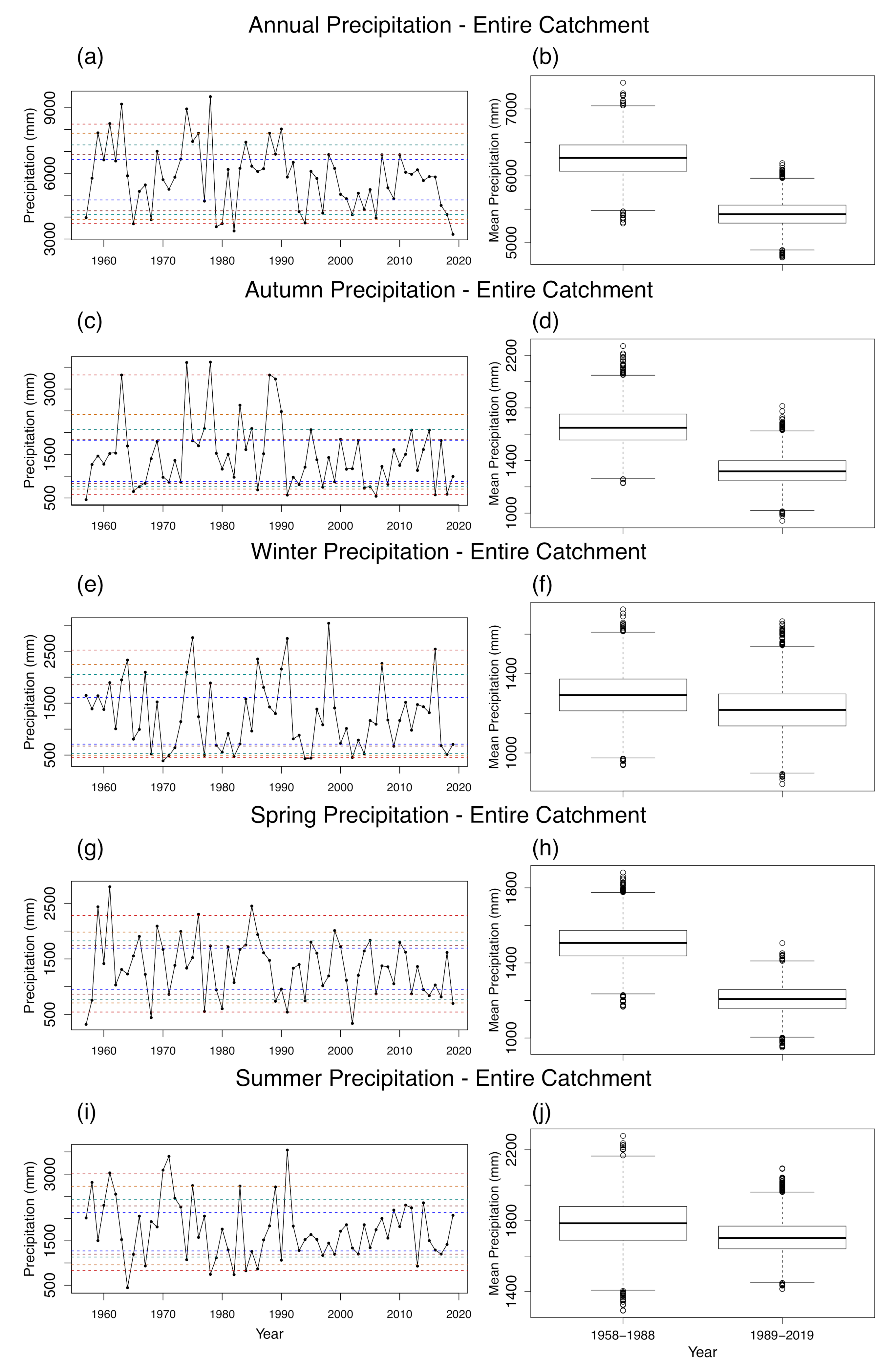
3.1. Evolution of Precipitation

Time series of annual precipitation and box plots of bootstrapped mean annual precipitation over the 31-year periods 1958–1988 and 1989–2019, for the SCA, are shown in Figure 3. Data presented in Figure 3 are annual (a,b) and cover the four seasons (c–j). In addition, p-values from permutation testing comparing the means and variances for the period 1958–1988 against 1989–2019 are presented in Table 2.
A significant decline in annual precipitation is apparent across the catchment, with a reduction in years recording above the 75th percentile since the 1990s, with only two years recording above the 75th percentile since the 2000s. Additionally, there is an increase in the frequency of years recording below the 25th percentile (Figure 3a). The most recent dry period is pronounced, with annual precipitation recording below the 25th percentile for the last three years, and 2019 in particular recording the lowest total annual precipitation over the observation period. This decline in annual precipitation is apparent in the 31-year box plots, exhibiting a statistically significant decrease in precipitation from a mean of approximately 6300 mm in 1958–1988 to a mean of 5400 mm during 1989–2019 (p-value = 0.0258; Figure 3b and Table 2). This decrease in annual mean precipitation is also accompanied by a statistically significant reduction in variance, as evidenced by the reduced lengths of the interquartile range and whiskers on the box plots (p-value = 0.028; Table 2).
The decreasing precipitation trend also is apparent for autumn (March–May) precipitation, with a statistically significant difference in mean precipitation between the two 31-year periods, greater than the 90% confidence level (p-value = 0.0778; Table 2 and Figure 3d). This reduction is evident in the time series, with no years recorded above the 90th percentile since 1990 and an increase in years recording below the 25th percentile since 1990 (Figure 3c). There appears to be a reduction in precipitation variance, with reduced interquartile range in the box plots; however, this is not statistically significant with a p-value = 0.218 (Table 2). In contrast, winter (June–August) precipitation appears relatively stable. There is a decrease in the number of years recording above the 75th percentile since the 1990s, although all but one of the years with winter precipitation above the 95th percentile occured during this period (Figure 3e). There also is little change to the frequency of years recording below the 25th percentile. This corresponds to only a slight decrease in winter precipitation in the 31-year period 1989–2019 that is not statistically significant (p-value = 0.685; Table 2 and Figure 3f).
There is another statistically significant decrease in spring (September–November) precipitation (p-value = 0.0228; Table 2 and Figure 3h). This is consistent with a reduction in years above the 75th percentile, and particularly years above the 90th percentile, from the 1990s (Figure 3g). There has also been an increased frequency of years below the 25th percentile since this time; however, years below the 10th percentile have reduced in frequency. This has resulted in a statistically significant reduction in variance of spring precipitation (p-value = 0.0802; Table 2 and Figure 3h). Meanwhile, there has been little change to mean summer precipitation (Figure 3j). However, the extremes of summer precipitation occurred less frequently from the 1990s with only one year recorded above the 95th percentile and one year below the 10th percentile in the last 30 years (Figure 3a). As such, the variance of summer precipitation is much reduced, with little variation around the mean (p-value of difference in variance between 1958–1988 and 1989–2019 = 0.0438; Table 2).
When splitting precipitation into the northern and southern catchment regions, it is apparent that the precipitation trends observed over the entire SCA are occurring in both regions (not shown). However, the trends in the northern catchment are not as substantial. The overall trend of decreasing annual precipitation (p-value = 0.0258, Table 2) over the SCA will increase pressure on water resources, especially as the population continues to increase. Although winter precipitation remains stable, the statistically significant reduction in autumn precipitation (p-value = 0.0778) is particularly of concern, as autumn precipitation is necessary to saturate the soil for winter and spring runoff [29,30]. The cooler months of the year are those when runoff is greatest in southeast Australia [31], and the decreasing trends in both autumn and spring precipitation suggest a trend to much reduced runoff in the future.

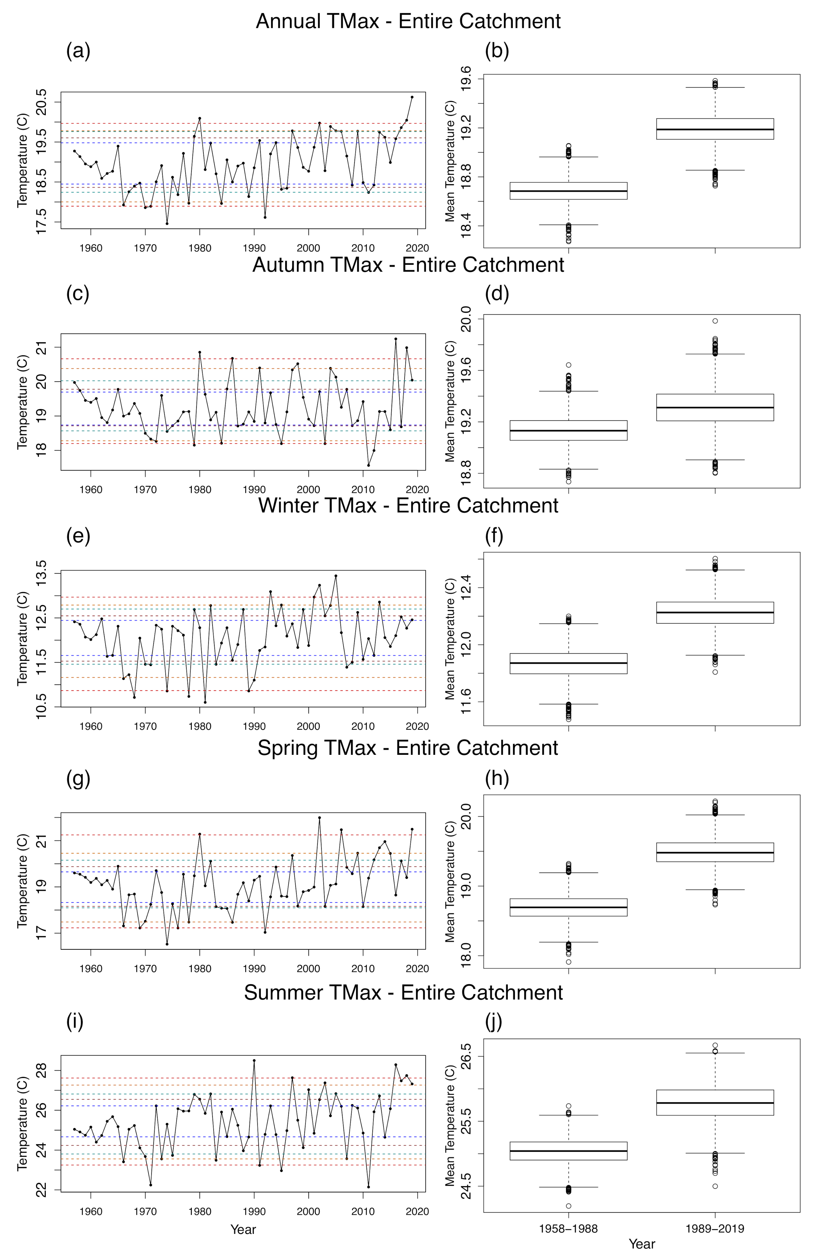
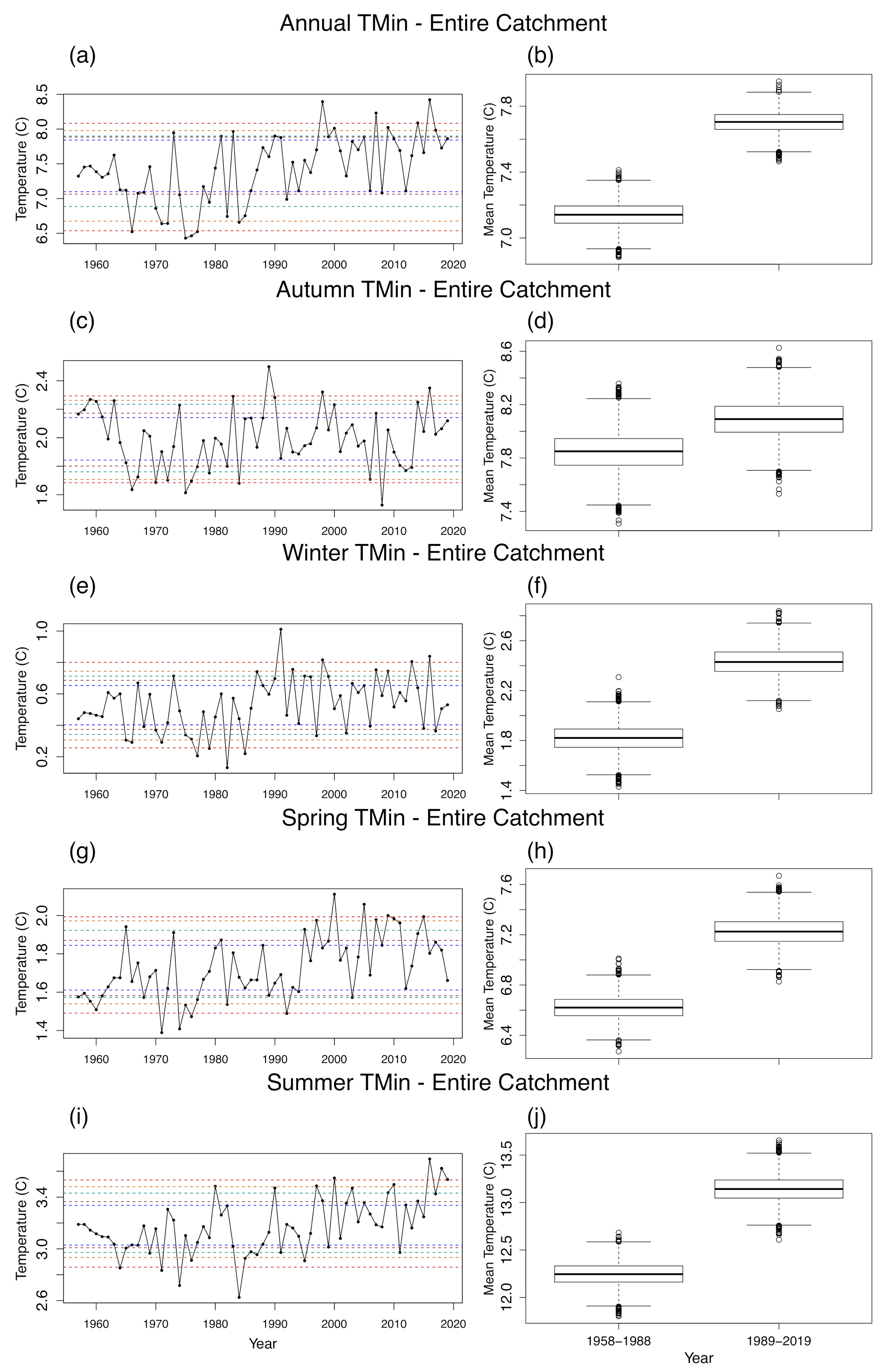
3.2. Evolution of Temperature

Figure 4 provides the time series and box plots of TMax annually and over the four seasons, while Figure 5 provides this overview for TMin. Understanding changes in temperature is important, as temperature influences potential evapotranspiration [10,29,30,31], and there is a non-linear relationship between temperature and precipitation with higher mean temperatures reducing precipitation during drought [12].
Annual TMax displays a clear increasing trend with a reduction in years below the 25th percentile since the 2000s and a corresponding increase in years above the 75th percentile (Figure 4a). This trend is statistically significant, with a p-value = 0.0036 (Table 2, Figure 4b). The last three years stand out, with TMax recorded above the 90th percentile in 2017, and the 95th percentile in 2018 and 2019 (Figure 4a). In particular, 2019 recorded the warmest catchment-average TMax over the period 1957–2019 of approximately 20.6 C, which is 1.7 C above the mean for the period of approximately 18.9 C. This increasing trend in TMax occurs across all seasons except autumn, where the increase in mean is not statistically significant (p-value = 0.36; Table 2 and Figure 4d). However, variance of mean TMax appears to have increased in autumn with a greater interquartile range in the 1989–2019 box plot. This change in autumn variance is statistically significant at the 90% confidence level (p-value = 0.0914; Table 2). There are similar, statistically significant, changes to variance of TMax in summer as displayed in the box plots (p-value = 0.0408; Table 2 and Figure 4j).
There is a noticeable increasing trend in annual TMin, with all years above the 90th percentile occurring since the late 1990s and a reduction in years recorded below the 25th percentile (Figure 5a). The change in annual TMin is statistically significant (p-value = 0.0000; Table 2) which is highlighted in the box plot figures where there is no overlap between the two 31-year periods (Figure 5b). Similar to TMax, the increase in TMin is statistically significant for all seasons except autumn (autumn p-value = 0.2470, while p-value for all other seasons <0.0004; Table 2 and Figure 5d). There are hints that autumn TMin might be starting to increase, with a reduction in the number of years recording below the 25th percentile since the 1990s, except for the late-2000s and early-2010s, and an upward shift in the 1989–2019 box plot with no statistically significant change in variance (Figure 5c).
Since both TMax and TMin are increasing across all seasons except autumn, it appears that mean temperatures are increasing across the SCA. This suggests further reductions in runoff and increased evapotranspiration even without the reduction in annual precipitation. Although little change in autumn mean temperature suggests evapotranspiration will remain much the same during this season, the reduced precipitation during autumn will influence runoff later in the year which will be further compounded by increases in mean temperature.

3.3. Wavelet Analysis of Precipitation

Global and local wavelet power spectra for precipitation in the SCA both annually and over the four seasons are provided in Figure 6. Annual precipitation displays statistically significant high global power over the 2–4 year period, which is suggestive of an ENSO influence on annual precipitation (Figure 6b). The ENSO signal is apparent to the late-1980s; however, it has weakened in the most recent 30 years. There also is indication of an interdecadal influence on annual precipitation with high global power over the 8–16 year period, which is partially in the 90% confidence band. This is reflected in the local wavelet power spectra where there is statistically significant power over the 8–16 year period between the 1960s and 1990s, and weak power from the 1990s onwards.
The ENSO influence on precipitation is apparent in all seasons globally, with statistically significant power over the 2–4 year period (Figure 6d–j). This influence is maintained throughout the time series for winter and spring (Figure 6e,g). However, the influence has greatly weakened from the 2000s in both autumn and summer precipitation (Figure 6c,i). The 8–16 year periodic signal is strongest in winter, with high power between 1970–2010 causing a statistically significant peak in the global power spectra (Figure 6e,f). There also is some high power over this period in the other seasons, although this is generally not statistically significant except between the late-1970s and early-1990s in spring (Figure 6g), and the 1960s to early-1970s in summer, the latter of which is outside the cone of influence (Figure 6i).

3.4. Wavelet Analysis of Temperature

Local and global wavelet power spectra were also computed for TMax and TMin and are presented in Figure 7 and Figure 8, respectively. There is statistically significant power over the 2–4 year period for TMax, which remains throughout the time series (Figure 7). This is visible throughout all seasons and displays little temporal change, although the signal only appears in autumn TMax from the late-1970s (Figure 7c). Additionally, the power for TMax in summer increases from the 1980s (Figure 7i).
Similarly, there is statistically significant power over the 2–4 year period for annual TMin, although this appears weaker than TMax over the global power spectrum (Figure 7b and Figure 8b). This also is noticeable in the local power spectra, with less continuity of statistically significant periodicities throughout the time series (Figure 8a). Annual TMin also displays a statistically significant signal in the 8–12 year period between the late-1970s and mid-1990s, which is suggestive of some interdecadal influence on annual TMin. This is nearly strong enough to reach the 90% confidence level in the global power spectrum (Figure 8b). High power over the 2–4 year period occurs over all four seasons (Figure 8d–j), although it is non-existent during summer before the 1970s (Figure 8i). The interdecadal signal in annual TMin appears mostly influenced by a statistically significant periodicity during summer over a similar time period (Figure 8a,i).
Overall, it appears that both TMax and TMin are influenced by ENSO although the ENSO influence on TMin is weaker. This influence generally holds throughout all seasons and has only small temporal changes, mainly during autumn and summer.

3.5. Attribution and Prediction of Annual Precipitation

For prediction of annual precipitation, the LR model that performed best is described by the equation:
Precipitation = 5887.4 941.8 × Ni ñ o 3.4 5339.1 × DMI × TSSST + ε ,
where ε represents the model error (some standard diagnostic plots, such as Q-Q and scale-location plots, were checked with no significant pattern displayed by the residuals to suggest the LR model could be significantly improved). The Poly SVR model used similar predictors to the LR, choosing Niño3.4, DMI*TSSST and Niño3.4*SAM, with free parameters C = 2 , G = 0.25 and E = 1 . Meanwhile, the RBF SVR model used a combination of GlobalT*Niño3.4 and SAM*TSSST as predictors, with C = 2 1.5 and G = 0.25 . The RF model used the predictors DMI*GlobalSSTA, DMI*GlobalT and DMI*SOI, with 150 trees. Shapiro–Wilks tests were applied to the residuals to test for normality, with p-values ranging from 0.21 to 0.25 for the four models. Therefore, it can be concluded that the residuals are normally distributed.
Table 3 displays the correlation, error statistics and skill scores for the final models on the testing data. The LR model achieved a high correlation of 0.815 (Table 3) but also had a relatively high RMSE of 764.971. Meanwhile, there was a slight decrease in correlation for the RBF SVR model to 0.761, but an improvement in RMSE by approximately 15% to 651.478. The best performing model is the Poly SVR, with an RMSE of 613.704 and high correlation of 0.921 (Table 3). Furthermore, the skill score of 0.721 of the Poly SVR suggests great improvement in results compared to the mean climatology. In contrast, the worst performing model was the RF model, which obtained an RMSE of 780.455 and correlation 0.622 (Table 3). Although the RF model underperforms compared to others, the skill score of all models is positive, and at least 0.55 (for the RF model; Table 3), which shows that all models greatly improve on predictions compared to the mean climatology.
Notably, both Poly SVR and LR models utilize the same predictors, except the Poly SVR has the added contribution of Niño3.4*SAM. Additionally, the kernel that was selected for the Poly SVR, after a grid search was performed, is essentially the linear kernel (i.e., E = 1 ). Looking at model predictions against observations, the climatology actually predicts annual precipitation fairly well until 2017 (not shown). This is unsurprising given annual precipitation does not appear to vary greatly over this part of the testing period, and remains approximately halfway between the 25th and 75th percentiles (Figure 3a). The greatest contribution to RMSE for the LR model is an underprediction in 2015 (not shown). The Poly SVR model improves on this, although it still underpredicts precipitation in 2015. This underprediction appears to be the result of a strongly positive Niño3.4 and SAM, which does not occur at any other point in the testing period (not shown). Both models closely predict the observed pattern of annual precipitation, including the significantly reduced precipitation over 2017–2019. However, the Poly SVR underpredicts 2019 precipitation more than the LR model. Both RBF SVR and RF models predict the shape of annual precipitation fairly well, including the reduced precipitation during 2017–2019, but they tended to overpredict precipitation over this period, which is not beneficial in preparing for drought.
Total precipitation over the northern and southern regions of the catchment also was modelled using the same approach as modelling precipitation over the entire SCA. Although these models performed relatively well e.g., the Poly SVR model on southern catchment precipitation obtained a correlation of 0.904 and skill of 0.66 (not shown), they did not collectively perform better than models of precipitation over the entire SCA. The best performing predictor sets from both northern and southern catchment models, however, were used in separate models of entire catchment precipitation to test if they performed better than models selected through forward selection on annual precipitation over the entire SCA. Interestingly, all models presented here, except the LR model, were formed using predictors that were part of either the northern or southern catchment precipitation models as these performed better than those selected using the traditional forward selection technique (not shown).

3.6. Attribution and Prediction of Autumn Precipitation

The best performing LR model for autumn precipitation is:
Precipitation = 1516.96 + 5121.52 × AMO × DMI 4477.40 × AMO × TSSST + ε .
Meanwhile, the RBF SVR used AMO*SOI, TPI*TSSST and Niño3.4*SAM as predictors, with C = 2 1.5 and G = 0.25 . The Poly SVR used predictors AMO*GlobalT, AMO*TSSST, GlobalSSTA*TPI and SAM, with C = 2 0.5 , G = 0.25 and E = 1 . The RF model used AMO*SOI, SOI*TPI and TPI as predictors, with 50 trees.
The LR model performs best for autumn precipitation, with an RMSE of 418.036 and a correlation of 0.679 (Table 4). The Poly SVR has an increase in RMSE of approximately 23% from the LR model, and achieves a much lower correlation of 0.493. There are further increases in RMSE for the RBF SVR and RF models. This results in both models having negative skill compared to the mean climatology of autumn precipitation (skill = −0.133 for RBF SVR, −0.226 for RF; Table 4). When comparing predictions against observations, all models largely tend to predict the shape of precipitation fairly well (not shown); however, the RF model often overpredicts precipitation while the other three models usually underpredict precipitation (Table 4). Of the observations in the testing set, only 2016 and 2018 recorded extremes in autumn precipitation. In these cases, both years were below the 90th percentile (Figure 3a). Of the models presented here, only the LR model predicts close to the 2016 observation, albeit underpredicting (not shown). Meanwhile both SVR models, particularly the Poly SVR model, predict close to the 2018 record.

3.7. Attribution and Prediction of Winter Precipitation

The best LR model for winter precipitation found through forward selection is:
Precipitation = 1310.47 + 1008.38 × SOI + 9843.28 × AMO × SAM 8858.67 × DMI × TPI + 4059.01 × SAM × TPI + ε .
The RBF SVR uses only AMO*GlobalSSTA and TPI as predictors, with C = 2 0.5 and G = 0.25 . The Poly SVR uses the predictors GlobalT*SOI, TPI*TSSST and TSSST, with C = 2 0.5 , G = 0.5 and E = 1 . The RF model uses AMO*SAM, DMI*TPI and Niño3.4*TPI, with 650 trees.
Here, the best performing model is the Poly SVR, which achieves an RMSE of 439.781 and a correlation of 0.703 (Table 5). The RBF SVR sees a decrease in correlation to 0.521, and increase in RMSE to 502.886. The LR and RF models perform fairly similarly, with LR having higher RMSE (533.319 compared to 522.228 for the RF model; Table 5) but also higher correlation of the predictions against observations (0.514 compared to 0.461 for the RF model). The LR model does not appear to capture the shape of precipitation over the testing period (2011–2019) very well (not shown). In contrast, the other models tend to capture the shape fairly well, especially the Poly SVR. These models were more inclined to underpredict precipitation whereas the LR model often overpredicted. The underprediction in the Poly SVR appears to mostly be related to the years 2015 and 2016. Precipitation during winter in 2016 was recorded above the 95th percentile, one of four years during the entire time series that recorded above the 95th percentile. The other three years were in the training data set; however, the model only appears to be trained relatively well to winter precipitation in 1998 (although still underpredicting, not shown).

4. Discussion

4.1. Drought Vulnerability

Global annual precipitation is expected to increase by approximately 7% per 1 C of warming due to changes in the atmosphere’s water-holding capacity [35]. A slight increasing trend in global precipitation has been observed; however, this is related largely to ENSO variability [36,37]. Despite the observed and expected increase in global precipitation, annual precipitation is decreasing in the SCA, due to a statistically significant decline in autumn and spring precipitation (p-values = 0.0778 and 0.0228, respectively; Table 2). There also is reduced variance in annual precipitation, due to decreasing variance in spring and summer. The decline in mean precipitation has been observed over southeast Australia and eastern Australia in previous studies, and is suggested to continue as a consequence of global warming causing the continued expansion of the Hadley cell, and reducing the frequency of rain-bearing systems reaching southern Australia [15,16,17,18]. Autumn precipitation is important for water catchment inflows over southeast Australia, because it saturates the soil for cool season runoff and evapotranspiration is lower during this period [29,30]. The decline in precipitation is further compounded by reductions in spring precipitation, which would result in notable reductions in runoff for the SCA.
Concomitant with the global warming trend [38], there is a statistically significant increase in mean TMax and TMin annually and over all seasons except autumn (e.g., annual p-values = 0.0036 for TMax and 0.0000 for TMin; Table 2). This general increase in mean TMax and TMin suggests mean temperatures across the catchment are also increasing. Increasing temperatures lead to increased evapotranspiration, which reduces water storages. Combined with the clear reduction in annual precipitation, it is likely that there will be future droughts that are potentially more intense than those that have been experienced in the past. Furthermore, future water resources for the Sydney region will be strained.

4.2. Attribution and Prediction

Although non-linear statistical models have proved valuable for the prediction of variables such as precipitation, and attribution of these variables with climate drivers [2,12,21,22,25], their use in Australian hydrological problems has been limited. This is especially the case for Australia’s most populous city, Sydney, where little has been published examining the applicability of non-linear models to predict and attribute annual and seasonal precipitation over the SCA. The most recent drought that affected the Sydney region, and resulted in tight water restrictions, highlights the importance of pursuing research into improving predictability of precipitation on various time scales for improved water management. In this study, multiple LR, SVR and RF were used with 10-fold cross-validation for attribution and prediction of annual precipitation, and precipitation during autumn and winter in the SCA. Two separate SVR models were developed, one used the radial basis function kernel (RBF) while the other used the polynomial kernel (Poly). The two seasons were selected to create precipitation models as runoff in this region of Australia typically is greatest during the cooler months of the year [31]. The northern region (Lithgow, Blackheath and Darkes Forest) typically records greater precipitation than the southern region (Moss Vale, Goulburn and Braidwood), suggestive of potential differences in the drivers of precipitation in these regions. Therefore, the catchment precipitation data also was split in order to develop models of precipitation for these regions. These models did not collectively perform better than models of the precipitation over the entire SCA, so they were not presented here. However, the predictors of the best performing models for the northern and southern catchments were also considered for all statistical models of precipitation over the SCA. This resulted in better models when compared to those selected through forward selection with 10-fold cross-validation on catchment-wide precipitation for three of the four annual precipitation models, and one of four winter precipitation models.
Overall, the Poly SVR performed best for prediction of annual and winter precipitation over the testing period (2011–2019), while the LR model performed best on autumn precipitation. Interestingly, when the Poly SVR performed best, the grid search for an optimal exponent yielded a kernel with degree one. This does not necessarily suggest the LR model will perform similarly, for example, although the LR model for annual precipitation performs fairly well (RMSE = 764.971 and correlation = 0.815; Table 3), it achieves a skill score that is approximately 21% lower than that of the Poly SVR. This is despite sharing all but one predictor in common with the Poly SVR. The results presented in this paper, where an SVR with a linear kernel or the LR model perform best on the data, reflect the moderately strong linear relationships between the predictors and annual precipitation shown in Figure 2. Although non-linear statistical models perform better than LR in some circumstances (e.g., [25]), and even perform somewhat better here, it is important to survey the performance of various statistical models as the results are dependent on location-specfic features.
For annual precipitation in the SCA, there are many common attributes. In fact, both the LR model and Poly SVR model chose DMI*TSSST and Niño3.4 as predictors, while the Poly SVR also included the interaction term Niño3.4*SAM. Niño3.4 and SOI are both indices related to ENSO. This attribute is included at least once in all models, highlighting the known strong influence of ENSO on precipitation in eastern Australia [39], which also was identified by the wavelet analysis (Figure 6). Additional influences on annual precipitation appear to be the DMI and a measure of global warming, typically the TSSST.
Attributes in common among the models predicting autumn precipitation include AMO, TPI and TSSST. Meanwhile, the winter precipitation models have AMO, TPI and predictors related to ENSO. It is notable that measures of global warming, including SST anomalies or global temperature anomalies, are included in the Poly SVR for winter precipitation, despite no clear trend in either the mean or variance of winter precipitation (Figure 3). The influence of ENSO on autumn and winter precipitation was identified by the wavelet analysis (Figure 6c–f), although the exclusion of predictors related to ENSO in the autumn precipitation models is likely due to the reduced influence of ENSO from the 1990s. Additionally, the wavelet analysis displays high periodicity over the 8–16 year period, with statistical significance for winter precipitation. This is likely why TPI was a common attribute among the autumn and winter precipitation models, and potentially why the AMO was selected, which has been shown to exert a decadal influence over ENSO [40,41,42]. The commonly selected attributes for precipitation during autumn and winter differ somewhat from those selected for annual precipitation, with the inclusion of AMO and TPI, and exclusion of DMI. This highlights how seasonal precipitation can be influenced by different climate drivers of annual precipitation.
Autumn and winter precipitation individually contribute approximately 25% and 21%, respectively, to the annual mean precipitation. Despite the selection of different climate drivers that might be more applicable for the individual seasons, the models for individual seasons do not perform better overall than the best performing annual precipitation model. For example, the RMSE for the best performing models in either autumn or winter is more than 50% of the RMSE for the best performing model of annual precipitation. This is likely because the variance between seasons is fairly large compared to annual precipitation, especially for winter, with the timing and location of east coast low events influential on the resulting precipitation in a season. Rather than being highly accurate models of seasonal precipitation, the models for individual seasons appear more suitable as indicators of whether the season is likely to be dry or wet, relative to the climatology (not shown).
ENSO influences the location of convection in the Pacific Ocean, with El-Niño events responsible for decreased convection over tropical Australia and a reduction of precipitation over eastern Australia [43,44]. The DMI also influences precipitation in eastern Australia, with large-scale moisture advection from the Indian Ocean feeding into precipitation bearing systems, such as northwest cloud bands [45,46]. During a negative DMI event, there is greater precipitation over eastern Australia, whereas a positive DMI is associated with cooler waters off the northwest of Australia and reduced precipitation in eastern Australia from reduced moisture advection. SST anomalies are considered a measure of global warming that is more reliable than the global temperature anomalies that include land surfaces due to reduced variability compared to the near-surface atmosphere [20]. As there is a decreasing trend in annual precipitation, it is not surprising that some form of SST anomalies are included as a predictor in each model, and SST anomalies might be favoured over global temperature anomalies because the ocean responds slower than land to global temperature change [47]. The selection of TSSST by the LR and Poly SVR models is likely because it is adjacent to the SCA, therefore it influences local moisture advection and precipitation on a smaller scale. The inclusion of the interaction between DMI and TSSST highlights a compound effect of the Indian Ocean and Tasman Sea on precipitation systems. The AMO and TPI were selected by numerous models on autumn and winter precipitation, generally as a two-way interaction with another variable. Previous studies have found Atlantic Ocean variability can influence tropical Pacific climate variability, modulating the global Walker circulation [40,41]. This has been found to influence Australian precipitation variability by altering sea-level pressure anomalies in the region [42]. The TPI (or interdecadal Pacific oscillation) influences rainfall over eastern Australia through varying the impact of ENSO on precipitation [48,49,50], likely through changes in the position of the South Pacific Convergence Zone [51]. The relationships between precipitation and the various climate drivers selected by the models are complex and future work is required to explore these relationships in detail, particularly for the effect of different climate drivers on autumn and winter precipitation in the region studied.
In this study, there was a general improvement in skill compared with climatology in modelling precipitation using either non-linear or linear statistical methods, particularly for annual precipitation where the skill score for the best performing model is 0.721 (Table 3). The importance of considering a range of statistical models, including linear models, is clear in this study as linear models sometimes outperform the non-linear techniques, or a linear kernel outperforms the non-linear RBF kernel in SVR. Neither the RBF SVR or RF models performed best in modelling precipitation, which raises the question of whether it is worthwhile considering these models in the future. Although they didn’t perform the best, they still performed comparatively well except in modelling autumn precipitation. Additionally, they selected attributes of precipitation that were similar to those selected by the better performing LR or Poly SVR models, suggesting that underlying physical relationships are being captured by the models rather than random relationships between the variables. Through forward selection, all models included at least one two-way interaction term, indicating the need to consider not only singular indices but also potential relationships between indices including multiplicative and possibly inverse relationships.
It was expected that splitting the precipitation time series into seasons and creating models for autumn and winter precipitation would improve predictability. However, this did not occur with the RMSE of these models being more than half that of the worst performing annual precipitation model. Future work should investigate how to improve this, as precipitation over the cooler months of the year are highly important for catchment inflows. In this study, only forward selection was applied to determine the predictors used in the models. However, this does not necessarily yield an optimal model from the subset of predictors [28]. This was clear after some optimal models for entire catchment precipitation were selected from the predictors used to model precipitation in either the northern or southern regions of the catchment. Therefore, one approach could be to employ a wider range of selection techniques, such as correlation-based feature selection [52]. Another approach could be to investigate the use of lagged time series of climate predictors, which proved beneficial in previous drought modelling studies (e.g., [53]). Finally, as found in Section 3.1, precipitation in the SCA is non-stationary. It is expected that relationships with climate variables will change as global warming continues [54]. Despite the high performance of models in this study, the predictors that were useful here might not be in the future. Therefore, there is a need to reassess the important attributes to SCA precipitation and develop updated models that are relevant to future climate regimes.

5. Conclusions

This study found that annual precipitation over the Sydney catchment area (SCA) is decreasing in the 31-year period 1989–2019, due to a decline in precipitation during both autumn and spring from the 1990s. This decrease in precipitation is expected to continue with the global warming trend. In addition, mean temperature over the SCA displayed an increasing trend over all seasons except autumn. This suggests the SCA is going to be increasingly vulnerable to drought conditions in the future. Further strain will be placed on water supply as the population continues to increase [19]. Therefore, it is necessary to continue monitoring trends in variables associated with water supply, and improve water supply through infrastructure investment and better seasonal forecasting.
In this study, multiple linear regression (LR), support vector regression (SVR) and random forests (RF) were used to model annual, autumn and winter precipitation. The models highlighted the importance of DMI, ENSO and Tasman Sea SST anomalies on annual precipitation. Different attributes were found to be associated with autumn precipitation (AMO, TPI and TSSST) and winter precipitation (AMO, TPI and ENSO). However, the models of autumn and winter precipitation did not perform as well as annual precipitation, with model errors individually more than 50% greater than those for annual precipitation. The models of autumn and winter precipitation appeared to be better used as indicators whether that season would likely be wetter or drier than average.
Overall, the models performed very well, with clear links between climate indices and annual, autumn and winter precipitation, despite the observed trends in annual and autumn precipitation. By performing studies using linear and non-linear statistical modelling, among other methods, the complex relationships between climate indices and atmospheric variables can be better understood. This can improve the application of climate driver indices in seasonal forecasts of atmospheric variables such as precipitation and temperature, which are performed by national weather agencies including the Australian Bureau of Meteorology, UK Met Office and National Weather Service. The best performing models in this study, depending on season, were either LR or the Poly SVR with an exponent of one. This highlights how linear models compare with non-linear models, and the importance of testing a wide-range of modelling techniques when developing a statistical model, rather than assuming that one model will perform better than another.

Author Contributions

Conceptualisation, S.M. and L.M.L.; methodology, J.H., S.M. and L.M.L.; software, J.H.; formal analysis, J.H.; investigation, J.H.; data curation, J.H.; writing—original draft preparation, J.H.; writing—review and editing, J.H., S.M., L.M.L. and M.S.; visualisation, J.H.; supervision, S.M. and L.M.L. All authors have read and agreed to the published version of the manuscript.

Funding

This research is supported by an Australian Government Research Training Program Scholarship. Shev MacNamara acknowledges funding from the Australian Research Council Centre of Excellence for Mathematical and Statistical Frontiers and the School of Mathematical and Physical Sciences, University of Technology Sydney.

Acknowledgments

We thank three anonymous reviewers for their feedback which has improved the quality of the manuscript.

Conflicts of Interest

The authors declare no conflict of interest.

Data Availability

Data sets related to this article can be found at https://0-doi-org.brum.beds.ac.uk/10.5281/zenodo.4037473 hosted at Zenodo [55].

References

  1. Kiem, A.S.; Johnson, F.; Westra, S.; van Dijk, A.; Evans, J.P.; O’Donnell, A.; Rouillard, A.; Barr, C.; Tyler, J.; Thyer, M.; et al. Natural hazards in Australia: Droughts. Clim. Chang. 2016, 139, 37–54. [Google Scholar] [CrossRef]
  2. Richman, M.B.; Leslie, L.M. Machine Learning for Attribution of Heat and Drought in Southwestern Australia. Procedia Comput. Sci. 2019, 168, 3–10. [Google Scholar] [CrossRef]
  3. Mukherjee, S.; Mishra, A.; Trenberth, K. Climate Change and Drought: A Perspective on Drought Indices. Curr. Clim. Chang. Rep. 2018, 4, 145–163. [Google Scholar] [CrossRef]
  4. Cheeseman, J. Food Security in the Face of Salinity, Drought, Climate Change, and Population Growth. In Halophytes for Food Security in Dry Lands; Elsevier: Amsterdam, The Netherlands, 2016; pp. 111–123. [Google Scholar]
  5. Stanke, C.; Kerac, M.; Prudhomme, C.; Medlock, J.; Murray, V. Health Effects of Drought: A Systematic Review of the Evidence. PLoS Curr. 2013, 5. [Google Scholar] [CrossRef] [PubMed] [Green Version]
  6. Dowdy, A.; Pepler, A.; Di Luca, A.; Cavicchia, L.; Mills, G.; Evans, J.; Louis, S.; McInnes, K.; Walsh, K. Review of Australian east coast low pressure systems and associated extremes. Clim. Dyn. 2019, 53, 4887–4910. [Google Scholar] [CrossRef]
  7. Sydney Water. Sydney’s Drought: Aquabumps Shows Just How Dry it Got. 2020. Available online: https://www.sydneywater.com.au/SW/about-us/our-publications/Media/sydney-s-drought–aquabumps-shows-just-how-dry-it-got/index.htm (accessed on 1 August 2020).
  8. Bureau of Meteorology. The “Federation Drought”, 1895–1902. 2009. Available online: https://webarchive.nla.gov.au/awa/20090330051442/http://pandora.nla.gov.au/pan/96122/20090317-1643/www.bom.gov.au/lam/climate/levelthree/c20thc/drought1.html (accessed on 4 June 2020).
  9. The World War II Droughts 1937–1945. Available online: https://webarchive.nla.gov.au/awa/20090330051442/http://pandora.nla.gov.au/pan/96122/20090317-1643/www.bom.gov.au/lam/climate/levelthree/c20thc/drought3.html (accessed on 4 June 2020).
  10. Chiew, F.H.S.; Potter, N.J.; Vaze, J.; Petheram, C.; Zhang, L.; Teng, J.; Post, D.A. Observed hydrologic non-stationarity in far south-eastern Australia: Implications for modelling and prediction. Stoch. Environ. Res. Risk Assess. 2014, 28, 3–15. [Google Scholar] [CrossRef]
  11. Richman, M.B.; Leslie, L.M. Uniqueness and Causes of the California Drought. Procedia Comput. Sci. 2015, 61, 428–435. [Google Scholar] [CrossRef] [Green Version]
  12. Richman, M.B.; Leslie, L.M. The 2015–2017 Cape Town Drought: Attribution and Prediction Using Machine Learning. Procedia Comput. Sci. 2018, 140, 248–257. [Google Scholar] [CrossRef]
  13. Diffenbaugh, N.S.; Swain, D.L.; Touma, D. Anthropogenic warming has increased drought risk in California. Proc. Natl. Acad. Sci. USA 2015, 112, 3931–3936. [Google Scholar] [CrossRef] [Green Version]
  14. Niang, I.; Ruppel, O.C.; Abdrabo, M.A.; Essel, A.; Lennard, C.; Padgham, J.; Urquhart, P. 2014: Africa. In Climate Change 2014: Impacts, Adaptation, and Vulnerability. Part B: Regional Aspects. Contribution of Working Group II to the Fifth Assessment Report of the Intergovernmental Panel on Climate Change; Technical Report; Cambridge University Press: Cambridge, UK; New York, NY, USA, 2014; pp. 1199–1265. [Google Scholar]
  15. Speer, M.; Leslie, L.; Fierro, A. Australian east coast rainfall decline related to large scale climate drivers. Clim. Dyn. 2011, 36, 1419–1429. [Google Scholar] [CrossRef]
  16. Timbal, B.; Fawcett, R. A Historical Perspective on Southeastern Australian Rainfall since 1865 Using the Instrumental Record. J. Clim. 2013, 26, 1112–1129. [Google Scholar] [CrossRef]
  17. Timbal, B.; Drosdowsky, W. The relationship between the decline of Southeastern Australian rainfall and the strengthening of the subtropical ridge. Int. J. Climatol. 2013, 33, 1021–1034. [Google Scholar] [CrossRef]
  18. Post, D.A.; Timbal, B.; Chiew, F.H.S.; Hendon, H.H.; Nguyen, H.; Moran, R. Decrease in southeastern Australian water availability linked to ongoing Hadley cell expansion. Earth’s Future 2014, 2, 231–238. [Google Scholar] [CrossRef]
  19. Australian Bureau of Statistics. Australian Demographic Statistics; Technical Reportl Cat. No. 3101.0; Australian Bureau of Statistics: Canberra, Australia, 2019; 44p. [Google Scholar]
  20. Choudhury, D.; Mehrotra, R.; Sharma, A.; Gupta, A.; Sivakumar, B. Effectiveness of CMIP5 Decadal Experiments for Interannual Rainfall Prediction Over Australia. Water Resour. Res. 2019, 55, 7400–7418. [Google Scholar] [CrossRef]
  21. Deo, R.C.; Şahin, M. Application of the Artificial Neural Network model for prediction of monthly Standardized Precipitation and Evapotranspiration Index using hydrometeorological parameters and climate indices in eastern Australia. Atmos. Res. 2015, 161, 65–81. [Google Scholar] [CrossRef]
  22. Bagirov, A.M.; Mahmood, A.; Barton, A. Prediction of monthly rainfall in Victoria, Australia: Clusterwise linear regression approach. Atmos. Res. 2017, 188, 20–29. [Google Scholar] [CrossRef]
  23. Torrence, C.; Compo, G.P. A Practical Guide to Wavelet Analysis. Bull. Am. Meteor. Soc. 1998, 79, 61–78. [Google Scholar] [CrossRef] [Green Version]
  24. Lau, K.M.; Weng, H. Climate Signal Detection Using Wavelet Transform: How to Make a Time Series Sing. Bull. Am. Meteor. Soc. 1995, 76, 2391–2402. [Google Scholar] [CrossRef] [Green Version]
  25. Hartigan, J.; MacNamara, S.; Leslie, L. Application of Machine Learning to Attribution and Prediction of Seasonal Precipitation and Temperature Trends in Canberra, Australia. Climate 2020, 8, 76. [Google Scholar] [CrossRef]
  26. Vapnik, V. The Nature of Statistical Learning Theory; Springer: New York, NY, USA, 1995. [Google Scholar]
  27. Breiman, L. Random forests. Mach. Learn. 2001, 45, 5–32. [Google Scholar] [CrossRef] [Green Version]
  28. Hastie, T.; Tibshirani, R.; Friedman, J. The Elements of Statistical Learning: Data Mining, Inference, and Prediction; Springer Science & Business Media: New York, NY, USA, 2009. [Google Scholar]
  29. Cai, W.; Cowan, T. Dynamics of late autumn rainfall reduction over southeastern Australia. Geophys. Res. Lett. 2008, 35, L09708. [Google Scholar] [CrossRef]
  30. Cai, W.; Cowan, T.; Briggs, P.; Raupach, M. Rising temperature depletes soil moisture and exacerbates severe drought conditions across southeast Australia. Geophys. Res. Lett. 2009, L21709. [Google Scholar] [CrossRef]
  31. Kirono, D.; Chiew, F.; Kent, D. Identification of best predictors for forecasting seasonal rainfall and runoff in Australia. Hydrol. Process. 2010, 24, 1237–1247. [Google Scholar] [CrossRef]
  32. Maldonado, S.; Weber, R. A wrapper method for feature selection using Support Vector Machines. Inf. Sci. 2009, 179, 2208–2217. [Google Scholar] [CrossRef]
  33. Hsu, C.-W.; Chang, C.-C.; Lin, C.-J. A Practical Guide to Support Vector Classification; Technical Report; National Taiwan University: Taipei, Taiwan, 2003; p. 16. [Google Scholar]
  34. Wilks, D.S. Statistical Methods in the Atmospheric Sciences; Academic Press: San Diego, CA, USA, 2011; Volume 100. [Google Scholar]
  35. Trenberth, K. Changes in precipitation with climate change. Clim. Res. 2011, 47, 123–138. [Google Scholar] [CrossRef] [Green Version]
  36. Trenberth, K.; Dai, A.; van der Schrier, G.; Jones, P.; Barichivich, J.; Briffa, K.; Sheffield, J. Global warming and changes in drought. Nat. Clim. Chang. 2014, 4, 17–22. [Google Scholar] [CrossRef]
  37. Adler, R.; Gu, G.; Sapiano, M.; Wang, J.J.; Huffman, G. Global Precipitation: Means, Variations and Trends During the Satellite Era (1979–2014). Surv. Geophys. 2017, 38, 679–699. [Google Scholar] [CrossRef] [Green Version]
  38. Stocker, T.; Qin, D.; Plattner, G.K.; Tignor, M.; Allen, S.; Boschung, J.; Nauels, A.; Xia, Y.; Bex, V.; Midgley, P. Climate Change 2013: The Physical Science Basis. Contribution of Working Group I to the Fifth Assessment Report of the Intergovernmental Panel on Climate Change; Cambridge University Press: Cambridge, UK; New York, NY, USA, 2014. [Google Scholar]
  39. McBride, J.L.; Nicholls, N. Seasonal Relationships between Australian Rainfall and the Southern Oscillation. Mon. Weather Rev. 1983, 111, 1998–2004. [Google Scholar] [CrossRef]
  40. Kucharski, F.; Kang, I.S.; Farneti, R.; Feudale, L. Tropical Pacific response to 20th century Atlantic warming. Geophys. Res. Lett. 2011, 38, 5. [Google Scholar] [CrossRef] [Green Version]
  41. Kucharski, F.; Ikram, F.; Molteni, F.; Farneti, R.; Kang, I.S.; No, H.H.; King, M.; Giuliani, G.; Mogensen, K. Atlantic forcing of Pacific decadal variability. Clim. Dyn. 2016, 46, 2337–2351. [Google Scholar] [CrossRef]
  42. Johnson, Z.; Chikamoto, Y.; Luo, J.J.; Mochizuki, T. Ocean Impacts on Australian Interannual to Decadal Precipitation Variability. Climate 2018, 6, 61. [Google Scholar] [CrossRef] [Green Version]
  43. Bureau of Meteorology. Climate Glossary. 2012. Available online: http://www.bom.gov.au/climate/glossary/elnino.shtml (accessed on 1 August 2020).
  44. Ummenhofer, C.; Gupta, A.; Briggs, P.; England, M.; McIntosh, P.; Meyers, G.; Pook, M.; Raupach, M.; Risbey, J. Indian and Pacific Ocean Influences on Southeast Australian Drought and Soil Moisture. J. Clim. 2011, 24, 1313–1336. [Google Scholar] [CrossRef] [Green Version]
  45. Risbey, J.S.; Pook, M.J.; McIntosh, P.C.; Wheeler, M.C.; Hendon, H.H. On the Remote Drivers of Rainfall Variability in Australia. Mon. Weather Rev. 2009, 137, 3233–3253. [Google Scholar] [CrossRef]
  46. Ummenhofer, C.C.; England, M.H.; McIntosh, P.C.; Meyers, G.A.; Pook, M.J.; Risbey, J.S.; Gupta, A.S.; Taschetto, A.S. What causes southeast Australia’s worst droughts? Geophys. Res. Lett. 2009, 36. [Google Scholar] [CrossRef] [Green Version]
  47. Hansen, J.; Ruedy, R.; Sato, M.; Lo, K. Global Surface Temperature Change. Rev. Geophys. 2010, 48. [Google Scholar] [CrossRef] [Green Version]
  48. Power, S.; Casey, T.; Folland, C.; Colman, A.; Mehta, V. Inter-decadal modulation of the impact of ENSO on Australia. Clim. Dyn. 1999, 15, 319–324. [Google Scholar] [CrossRef]
  49. Verdon, D.; Wyatt, A.; Kiem, A.; Franks, S. Multidecadal variability of rainfall and streamflow: Eastern Australia. Water Resour. Res. 2004, 40, W10201. [Google Scholar] [CrossRef]
  50. Kiem, A.; Franks, S. Multi-decadal variability of drought risk, eastern Australia. Hydrol. Process. 2004, 18, 2039–2050. [Google Scholar] [CrossRef]
  51. Folland, C.; Renwick, J.; Salinger, M.; Mullan, A. Relative influences of the Interecadal Pacific Oscillation and ENSO on the South Pacific Convergence Zone. Geophys. Res. Lett. 2002, 29, 21–1–21–4. [Google Scholar] [CrossRef]
  52. Hall, M.A. Correlation-Based Feature Selection for Machine Learning. Ph.D. Thesis, University of Waikato, Hamilton, New Zealand, 1999. [Google Scholar]
  53. Prasad, R.; Deo, R.C.; Li, Y.; Maraseni, T. Input selection and performance optimization of ANN-based streamflow forecasts in the drought-prone Murray Darling Basin region using IIS and MODWT algorithm. Atmos. Res. 2017, 197, 42–63. [Google Scholar] [CrossRef]
  54. Benoit, L.; Vrac, M.; Mariethoz, G. Nonstationary stochastic rain type generation: Accounting for climate drivers. Hydrol. Earth Syst. Sci. 2020, 24, 2841–2854. [Google Scholar] [CrossRef]
  55. Hartigan, J. Precipitation and Temperature Data for the Sydney Catchment Area, Australia. 2020. Available online: https://0-doi-org.brum.beds.ac.uk/10.5281/zenodo.4037473 (accessed on 19 September 2020).
Figure 1. Location map of the Sydney catchment area (outline in dark grey): the six sites where data were obtained and the Sydney central business district (black dots).
Climate 08 00120 g001
Figure 2. Scatter plot of annual precipitation across the Sydney catchment area (SCA) against each climate driver that serves as a possible attribute. The thin black line shows a linear fit against the data using least squares regression. Correlations of each predictor against precipitation are provided in the box to the lower right of each sub-panel; low correlations ( | r | < 0.3 ) indicate a weak linear relationship between a predictor and precipitation.
Climate 08 00120 g002
Figure 3. (left panels, (a,c,e,g,i)) Annual precipitation time series summed across all six sites. Dashed lines indicate the 5th and 95th (bottom and top red), 10th and 90th (bottom and top orange), 15th and 85th (bottom and top green), 20th and 80th (bottom and top brown) and 25th and 75th percentiles (bottom and top dark blue); and (right panels, (b,d,f,h,j)) box plots of the bootstrapped mean annual precipitation over 31-year periods for the SCA.
Climate 08 00120 g003
Figure 4. (left panels, (a,c,e,g,i)) Annual mean TMax time series across the SCA; and (right panels, (b,d,f,h,j)) box plots of the bootstrapped mean TMax over 31-year periods for the SCA, as in Figure 3 but for mean TMax.
Climate 08 00120 g004
Figure 5. (left panels, (a,c,e,g,i)) Annual mean TMin time series across the SCA; and (right panels, (b,d,f,h,j)) box plots of the bootstrapped mean TMin over 31-year periods for the SCA, as in Figure 3 but for mean TMin.
Climate 08 00120 g005
Figure 6. Wavelet analysis for total precipitation across the Sydney catchment area both annually (a,b) and over the four seasons (cj). Low values (blue) in the wavelet power spectrum (left panels, (a,c,e,g,i)) indicate low periodicity, while high values (orange) indicate high periodicity. Horizontal peaks in the global power spectrum (right panel, (b,d,f,h,j)) indicate high periodicity over the time series. The dashed/solid red (black) line indicates the 95% (90%) confidence level in each plot. The cone of influence is depicted in the wavelet power spectrum by the solid black cone.
Climate 08 00120 g006
Figure 7. Wavelet power spectra (left panel, (a,c,e,g,i)) and global power spectra (right panel, (b,d,f,h,j)) for TMax, with low and high values in the power spectra indicating low and high periodicity, respectively; the cone of influence and statistical significance bands as already explained in Figure 6.
Climate 08 00120 g007
Figure 8. Wavelet power spectra (left panel, (a,c,e,g,i)) and global power spectra (right panel, (b,d,f,h,j)) for TMin, with low and high values in the power spectra indicating low and high periodicity, respectively; the cone of influence and statistical significance bands as already explained in Figure 6.
Climate 08 00120 g008
Table 1. Percentage of folds selecting attributes for precipitation in linear regression (LR); support vector regression (SVR) with the radial basis (RBF) and polynomial (Poly) kernel functions; and random forests (RF).
AttributeLRSVR (RBF)SVR (Poly)RFAttributeLRSVR (RBF)SVR (Poly)RF
AMO301008040DMI*TSSST90806020
DMI0708030GlobalSSTA*GlobalT0608010
GlobalSSTA0808030GlobalSSTA*Niño3.410608040
GlobalT80409020GlobalSSTA*TPI20608040
Niño3.460309020GlobalSSTA*SAM0907030
TPI10608030GlobalSSTA*SOI10609030
SAM20809020GlobalSSTA*TSSST0706030
SOI60608040GlobalT*Niño3.430409030
TSSST10309010GlobalT*TPI0609020
AMO*DMI60807040GlobalT*SAM01008050
AMO*GlobalSSTA10908040GlobalT*SOI10508030
AMO*GlobalT10807040GlobalT*TSSST10705050
AMO*Niño3.420507030Niño3.4*TPI0407030
AMO*TPI0705030Niño3.4*SAM40807030
AMO*SAM30809040Niño3.4*SOI0406030
AMO*SOI10809030Niño3.4*TSSST0407030
AMO*TSSST0506020TPI*SAM30708030
DMI*GlobalSSTA10108070TPI*SOI10507030
DMI*GlobalT10308050TPI*TSSST40507020
DMI*Niño3.450409040SAM*SOI0806040
DMI*TPI40607040SAM*TSSST201009050
DMI*SAM30808030SOI*TSSST10406040
DMI*SOI20708060
Table 2. p-values for the permutation test on the difference between the mean and variance of precipitation, TMax or TMin between 1958–1988 and 1989–2019, annually and across all four seasons. Tests conducted used 5000 resamples. Text in bold face highlights statistical significance at the 95% confidence level; text in italics highlights statistical significance at the 90% confidence level.
YearsPrecipitationTMaxTMin
Annual
Mean0.02580.00360.0000
Variance0.02800.25700.2300
Autumn
Mean0.07780.36000.2470
Variance0.21800.09140.8190
Winter
Mean0.68500.02260.0004
Variance0.84300.92900.7860
Spring
Mean0.02280.00700.0002
Variance0.08020.58400.2680
Summer
Mean0.63900.04400.0000
Variance0.04380.04080.3980
Table 3. Performance of each of the annual precipitation models on the testing data set (2011–2019). The best performing model for predicting annual precipitation is highlighted, determined by low RMSE, and both high correlation and skill.
ModelLRSVR (RBF)SVR (Poly)RF
RMSE (mm 2 )764.971651.478613.704780.455
Skill0.5670.6860.7210.550
Correlation0.8150.7610.9210.622
R 2 0.6630.5790.8480.387
Residuals Mean (mm)258.617−22.463310.67198.182
Residuals SD (mm)763.600690.585561.365821.221
Residuals Skewness1.3650.0840.5660.283
Residuals Kurtosis0.705−1.314−1.158−1.729
Table 4. Performance of each of the autumn precipitation models on the testing data set (2011–2019), similar to Table 3.
ModelLRSVR (RBF)SVR (Poly)RF
RMSE (mm 2 )418.036597.255515.242621.334
Skill0.445−0.1330.157−0.226
Correlation0.6790.1160.4930.094
R 2 0.4610.0130.2430.009
Residuals Mean (mm)118.211138.001162.255−112.422
Residuals SD (mm)425.297616.342518.692648.147
Residuals Skewness−0.545−0.360−0.0440.469
Residuals Kurtosis−0.856−0.864−1.148−1.414
Table 5. Performance of each of the winter precipitation models on the testing data set (2011–2019), similar to Table 3.
ModelLRSVR (RBF)SVR (Poly)RF
RMSE (mm 2 )533.319502.886439.781522.228
Skill0.1790.2700.4420.213
Correlation0.5140.5210.7030.461
R 2 0.2640.2720.4940.212
Residuals Mean (mm)−147.82758.190145.45267.985
Residuals SD (mm)543.506529.808440.207549.193
Residuals Skewness0.585−0.217−0.2051.009
Residuals Kurtosis−0.745−1.356−1.202−0.444
Publisher’s Note: MDPI stays neutral with regard to jurisdictional claims in published maps and institutional affiliations.

