Global-Scale Synchronization in the Meteorological Data: A Vectorial Analysis That Includes Higher-Order Differences

Abstract

To examine the evidence of global warming, in recent years, there has been a growing interest in the statistical analysis of time-dependent meteorological data. In this paper, for 116 observational stations in the world, sequential variations of the monthly distributions of meteorological data are analyzed vectorially. For specific monthly data, temperatures and precipitations are chosen, both of which are averaged over three decades. Climate change can be revealed through the intersecting angle between two 33-dimensional vectors being composed with monthly mean values. Subsequently, the angle data for the entire stations are analyzed statistically and compared between the former (1931–1980) and the latter (1951–2010) periods. Irrespective of the period and the hemisphere, the variation of the angles is found to show the exponential growth as a function of their latitudes. Furthermore, consistent with other studies, this trend is shown to become stronger in the latter period, indicating that the so-called snow/ice-albedo feedback occurs. In contrast to the temperatures, for the precipitations, no significant correlation is found between the angle and the latitude. To examine the albedo effect in more detail, a regional analysis for 75 stations in Japan is carried out as well. Numerical results show that the effect is significant even for the relatively narrow latitudinal range (19%) of the hemisphere. Finally, a synchronization of the monthly patterns of temperatures is given between the northern district of Japan and both North America and Eastern Europe.

1. Introduction

An agreement has been reached on the signs of global warming that have been found since the latter half of the former century [1,2]. Indeed, both the atmosphere and ocean have been getting warmer, the amounts of ice and snow have been decreasing, and the sea level has continued to rise. It has been shown that these were caused by the accumulating greenhouse gases due to human activity. In 2015, the concentration of carbon dioxide in the Earth’s atmosphere recorded 400 ppm [3], and at the same time, the mean temperature of the world became +1 °C higher than before the Industrial Revolution [4]. According to an estimation with the Representative Concentration Pathways (RCP) 8.5 scenario [2], it is reported that the difference attains to +2 °C in the early period of the present century, and furthermore, it attains up to +3 °C in the latter period of the century. In December of the same year, to present a long-term target for suppressing global warming, the Paris Agreement was adopted, and became effective in November of the subsequent year, when the Intergovernmental Panel on Climate Change (IPCC) had a large bearing upon its realization. Locally, warming may be accelerated at a rate higher than the estimation. Furthermore, it is predicted that so-called extreme meteorological phenomena, such as record-breaking temperatures as well as heavy rains will continue to be stronger in their scale and occur more frequently. Disasters due to climate change have started to be detected. For example, only recently has the Australian government reported the extinction of mammals similar to rats possibly because of the sea-level rising on an islet in the Great Barrier Reef. The increasing sea temperature is causing serious damage to the coral reef. Note that, along with the Marshall Islands in the east of the West-Pacific Micronesia, both the Great Barrier Reef along the east coast of Australia and the reef in the vicinity of the Okinawa Island of Japan are now in a critical condition. In the latter case, the coral bleaching has been arising from the rising sea temperature. Although the damage may not be so critical as that responsible for the extinction of an endangered species, reports of heatstroke are increasing substantially in the summer of Japan, where wet heat waves exceeding 35 °C continue sporadically for many days. To reduce the mortality risk of runners, the Tokyo 2020 Olympic Games Organizing Committee set the starting time of the marathon race at 6:00 a.m., which is substantially earlier than in the 1964 Tokyo Olympics. Furthermore, medical advisors suggested starting the race even earlier (5:30 a.m.) [5].

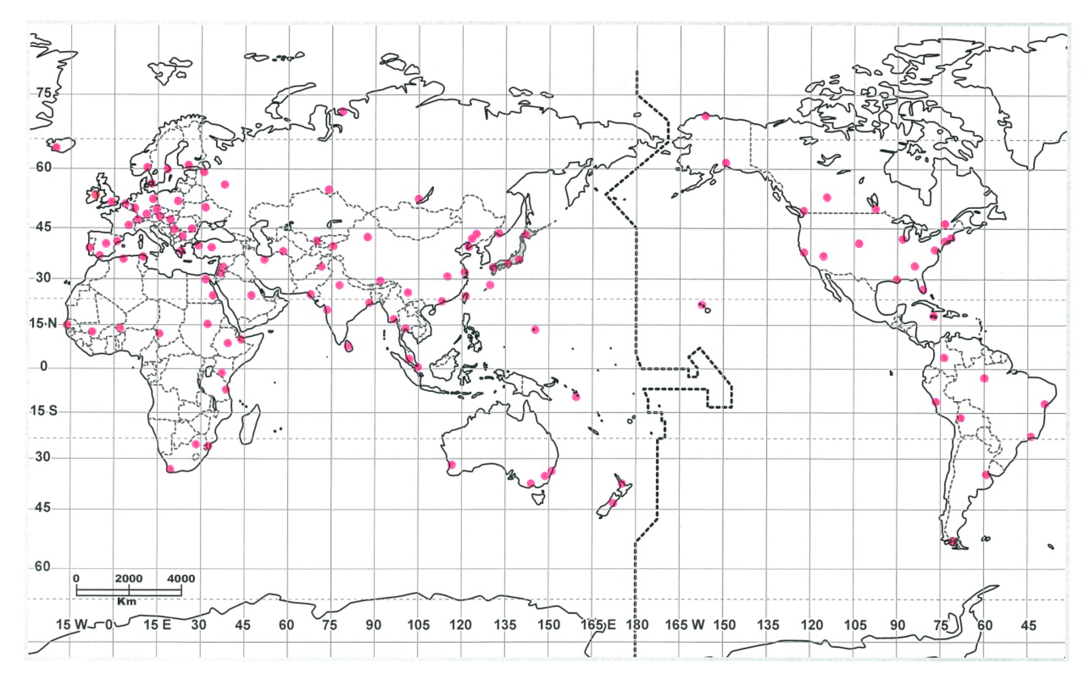
In recent years, not to mention the conventional fields such as geophysics, meteorology, climatology, aerometry, glaciology, and oceanography [6,7,8,9,10,11,12,13,14,15,16,17,18,19,20,21,22,23,24,25,26,27,28,29,30,31,32,33,34,35,36,37,38,39,40,41,42,43,44,45,46,47,48,49], a large number of research articles concerning climate change and/or global warming have also been published in the context of statistical physics [50,51,52,53,54,55,56,57,58,59,60,61,62,63,64,65]. The methodologies worth noting range over the method of detrended fluctuation analysis (DFA) [51], a variationally optimized Markov analysis combined with a successive over-relaxation algorithm [52], Monte Carlo simulations [53,56,57], feedforward artificial neural networks [54], convergent cross mapping (CCM) [59], wavelet transformation method [60], the method using Mahalanobis distance metrics [61], multifractal temporally weighted detrended fluctuation analysis [63], horizontal multivariate singular spectral analysis techniques [64], and the formalism of pitchfork bifurcation with the Lyapunov exponent [65]. In this paper, for 116 observational stations in the world (97 in the Northern Hemisphere and 19 in the Southern Hemisphere, as dotted on the map in Figure 1), sequential variations of the monthly distributions of meteorological data are analyzed vectorially. For specific monthly data, precipitations as well as temperatures are chosen, both of which are averaged over thirty years. According to the chronology [66,67,68] the entire eighty years are segmented into three periods: I: 1931–1960, II: 1951–1980, and III: 1981–2010. Climate change can be revealed through the cross angle between two twelve-dimensional vectors being composed with monthly mean values. In addition to the World temperature, analysis is made for the precipitation. Subsequently, in order to discuss the albedo feedback in detail, a regional analysis is carried out. The snow/ice-albedo effect can be explained by a positive feedback of enhanced light absorption due to the degenerate cover of snow and ice [1,2,69]. Specifically, 75 observational stations in Japan, which cover from Naze (28°23′ N, 129°30′ E) to Wakkanai (45°25′ N, 141°41′ E), are considered. While the longitudinal range of the spots approximately covers Darwin (130°50′ E) to Cairns (145°47′ E), latitudinally, the range is confined in Montreal (45°28′ N) to Cape Canaveral (28°23′ N) or in Lyon (45°43′ N) to Las Palmas de Gran Canaria (28°06′ N), the Islas Canarias. It is interesting to investigate whether the effect is significant even for the relatively narrow latitudinal range (19%) of the hemisphere. Finally, a synchronization of the monthly patterns of temperatures is given between selected spots in Japan and those in North America as well as Eastern Europe.

2. Methodology

In this paper, to enhance the precision and to avoid the production of a number of tie data (data having the same value), additional 21 components consisting of eleven first-order and ten second-order differences are included in each vector composed with monthly mean values. With this extension, one eventually obtains the 33-dimensional vector. Besides the simple linear regression [70,71,72], in order to examine the sign of the curvature, nonlinear regressions [73] are adopted. Identifying the (plus or minus) sign of curvature of the data as a function of the latitude is of particular concern for finding evidence of the warming.

2.1. Modified Vectorial Analysis

We consider two vectors p and q being composed by twelve components

p = (<u₁>, <u₂>, …, <u₁₂>),

(1)

q = (<x₁>, <x₂>, …, <x₁₂>).

(2)

where <u_i> and <x_i> (i = 1, 2, …, 12, for January to December) represent monthly mean values of the meteorological quantities such as temperatures and precipitations (for specific numeric, see, e.g., Equations (S1) and (S2) in Supplementary Material); the values are averaged further over the three decades. The intersecting angle between the vectors can be obtained by

θ= arccos [(p·q)/(|p||q|)],

(3)

where p·q indicates the scalar product between p and q. For instance, for p and q being produced with monthly averaged temperature distributions in the two subsequent periods (Period I to II or Period II to III), climate change between the periods can be evaluated by the magnitude of the angle. This procedure, however, is not free from disadvantage, because a number of quasi-tie data are generated, which might be responsible for making the subsequent statistical analysis ill-conditioned. To avoid this situation, in Equation (1) we join the second-order as well as the first-order differences

p = (<u₁>, <u₂>, …, <u₁₂>; <v₁>, <v₂>, …, <v₁₁>; <w₁>, <w₂>, …, <w₁₀>),

(4)

q = (<x₁>, <x₂>, …, <x₁₂>; <y₁>, <y₂>, …, <y₁₁>; <z₁>, <z₂>, …, <z₁₀>),

(5)

<v_j > = <u_j+1> − <u_j>, <w_k> = <v_k+1> − <v_k>,

(6)

<y_j > = <x_j+1> − <x_j>, <z_k> = <y_k+1> − <y_k>.

(7)

Here, j = 1, 2, …, 11 and k = 1, 2, …, 10. Note that <v_j > and <y_j> represent the rate of change whereas <w_k> and <z_k> imply the ‘monthly variation of curvature.’ In comparison between the monthly patterns bearing a close resemblance, besides the first-order difference the inclusion of the second-order difference is useful for discriminating their details. Although an unlimited extension to joining much higher-order differences is possible, no one can find the physical meaning of the numerical artifacts. In this paper, we concentrate on the relatively slowly varying patterns and do not deal with chaotic sequences as seen in the climate oscillations. In Equations (4) and (5), the independence among components is no longer ensured. It should be noted here that, as our method does not require the calculation of the eigenvector, the loss of independence is not as important as in the principal component analysis (PCA) [70], in which it is necessary to strictly preserve the orthogonalities among components of a vector. Upon the substitution of Equations (4) and (5) into Equation (3), one can improve the method substantially. Eventually the climate change between two periods as well as between two stations can be detected by calculating the rotation angle between the vectors p and q defined in the 33-dimensional co-ordinate. It seems that the present method with the rotation of the angle is useful for revealing potential synchronizations between meteorological data, along with the one using the Minkowski distance D_r between the two vectors; with a parameter r the distance is reduced to the city-block (L₁, taxicab, Manhattan, or more generally Bray–Curtis, Canberra, and Lance–Williams), the Euclidean, and the Chebyshev distance, respectively, for r = 1, 2, and ∞. Only recently have the Minkowski distance functions been used to detect teleconnections between temperatures, aerosol optical paths, and precipitation time series [74].

2.2. Statistical Analysis

Subsequently the angle data θ_i (i = 1, 2, …, n; n being the number of observational stations) will be dealt with statistically. Below, as specific regressions on the angles versus the coordinates, three functions are chosen:

Linear regression: θ= a + bχ,

(8)

Exponential regression: lnθ = a + b χ,

(9)

Logarithmic regression: θ= a + b lnχ,

(10)

where ln abbreviates the natural logarithm; χ represents the coordinate of the station; a and b are real constants to be determined with the least square fit, specifically a = m_Y − b m_X and b = s_XY/s_X²; (X, Y) = (χ, θ), (χ, lnθ), and (lnχ, θ) for Equations (8), (9), and (10), respectively. Here, m_Y (m_X), s_XY, and s_X², respectively, are the arithmetical mean of Y (X), the covariance of X and Y, and the variance of X. It should be emphasized here that the regressions can deal not only with the simple linearity (Equation (8)) but with the growth (Equation (9) with a positive curvature) as well as the saturation model (Equation (10) with a negative curvature). The validity of the present regression model can be checked by using the degree of fit, |r|, with the Pearson’s formula r = s_XY/ (s_X s_Y ) (0 < |r| < 1; s_Y² represents the variance of Y.), together with the Durbin–Watson ratio, d (0 < d < 4) [70,72].

d = (n − 2)⁻¹ Σ(ε_i+1 − ε_i) ²,

(11)

with the summation Σ for i = 1 to n − 1;

ε_i = e_i/s, e_i = Y_i − Ŷ_i, s² = (n − 2)⁻¹ Σe_i ²,

(12)

with the summation Σ for i = 1 to n. Here, n indicates the summation of regression points; the hat on Y represents the point on the regression line. With level alpha test being done, it can be judged that if 0 < d < d_L (d_L is the lower critical value) there exists a positive correlation between adjacent points on the sequence of the residual data e_i (i = 1, 2, …, n) and that if d_U < d ≤ 2 (d_U is the upper critical value) there is no correlation between them. Note that, for d_L ≤ d ≤ d_U, any judgment is impossible. Therefore, a null hypothesis that ‘H: there is a correlation between the neighboring residual data’ is rejected solely for d_U < d ≤ 2. (For d > 2, d must be replaced by 4 − d.) For typical levels the two critical values are obtainable from numerical tables available. In this paper the level 1% test, i.e., α= 0.01, will be adopted.

In what follows, the angle data generated for the entire stations on the map of Figure 1 are analyzed and are compared between the former (I/II: 1931–1980) and the latter (II/III: 1951–2010) period. If the trend obeys the exponentially growing curve with a positive curvature in the plot of the divergence versus the latitude, and at the same time its trend is shown to become stronger in the latter period, one can give hard evidence to show that the so-called snow/ice-albedo effect due to the positive feedback [1,2,69] may be responsible for the global warming.

3. Data

All the meteorological data employed in this paper are taken from a series of the Chronological Scientific Tables [66,67,68], which have over more than ninety years been edited by the National Astronomical Observatory, Japan. The observation points in the Tables were sampled without bias by the editors using Observing Stations, published by the World Meteorological Organization (WMO). By the Japan Meteorological Agency, both the temperature and the precipitation data are averaged over thirty years. Note that the original data were cited from those of the Global Historical Network, which were delivered by the National Climate Data Center (NCDC), USA, and from those of meteorological messages for monthly climatic variations, which had been received from meteorological organizations located all over the world. When necessary, data are supplemented with those of the National Center for Atmospheric Research (NCAR), USA. In Japan, the Tables have been winning broad support not only from researchers, engineers, and teachers, but from students and others engaged in science. Over the series of the Chronological Scientific Tables, the entire observational term is segmented into three periods: I (1931–1960) [66], II (1951–1980) [67], and III (1981–2010) [68]. Note that because of an uncertain editorial reason the former two periods overlap for 1951–1960; data of 1921–1950 are not available. In principle a complete survey is conducted and neither random nor intentional sampling is employed. The World observational stations are listed in Tables S1 and S2 in Supplementary Material, along with their coordinates and heights. In the Northern Hemisphere (Table S1), the latitudes range from 01°22′ N (Singapore) to 73°30′ N (Ostrov Dikson, Russia). Of the 97 stations, only the two spots (2%), #1: Ostrov Dikson and #2: Barrow, are located within the Arctic Circle (66°33′39″ N), whereas the 19 spots (20%), #79: Kolkata to #97: Singapore, are confined in the region between the equator and the Tropic of Cancer (23°26′21″N). In the Southern Hemisphere (Table S2), the latitudes cover 01°19′ S (Nairobi, Kenya) to 54°48′ S (Ushuaia, Argentina). Of the 19 stations, 8 (42%), #12: Rio De Janeiro to #19: Nairobi, are in the region between the equator and the Tropic of Capricorn (23°26′21″ S); there is no station within the Antarctic Circle (66°33′39″ S). The longitudinal distribution is (E, W) = (69, 28) and (12, 7), respectively. For the unit of temperature, the Celsius scale is adopted.

4. Results

4.1. Global Analysis

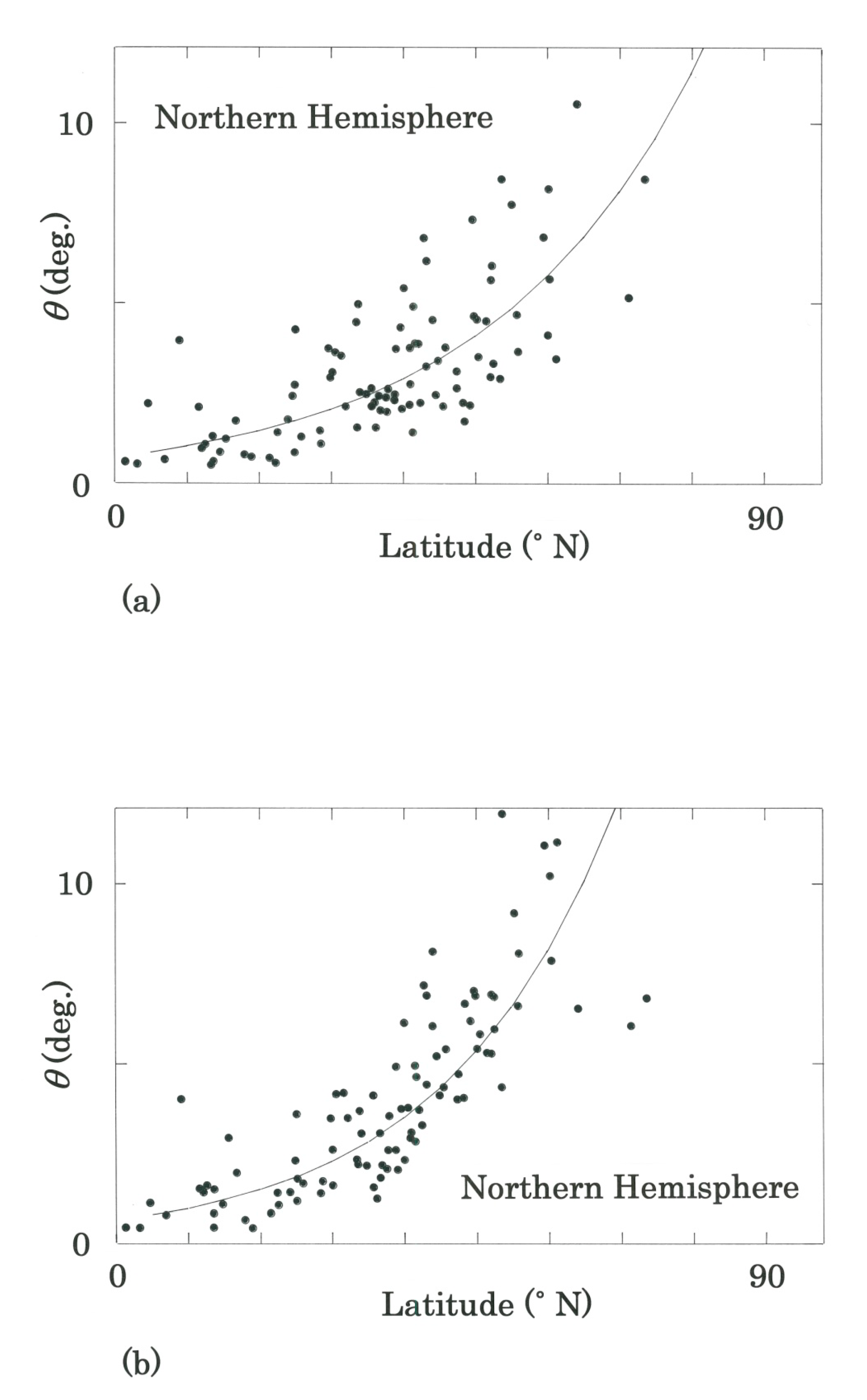
For monthly average temperature data, the dependence of the rotation angle on the latitude is plotted in Figure 2 for the Northern Hemisphere and in Figure 3 for the Southern Hemisphere. The top-thirty rankings of the rotation angle are given, respectively, in

Table 1. Top-thirty Northern Hemispheric stations in the rotation angle of the monthly distributions of temperatures from Period I (1931–1960) to II (1951–1980).

ΔT indicates the increment of the mean temperature from the former to the latter period.

and

Table 2. Top-thirty Northern Hemispheric stations in the rotation angle of the monthly distributions of temperatures from Period II (1951–1980) to III (1981–2010).

, and in

Table 3. Southern Hemispheric stations in the rotation angle of the monthly distributions of temperatures from Period I (1931–1960) to II (1951–1980).

and

Table 4. Southern Hemispheric stations in the rotation angle of the monthly distributions of temperatures from Period II (1951–1980) to III (1981–2010).

. For monthly averaged precipitation data, the top-thirty rankings of the angle are listed in Tables S3–S6 in Supplementary Material. With these results we conclude as follows:

(1)

In Figure 2a, which plots the rotation between Period I (1931–1960) and Period II (1951–1980), the best fit has been found to be exponential with r = 0.738 and d = 1.788 > d_U = 1.55 (n = 97). (cf. for the linear regression of Equation (8), r = 0.589 with d = 1.815.) It is evident from Table 1 that the top-thirty ranking is occupied by the stations with relatively high latitudes. Exceptions are #16: Atlanta (33°39′ N; h = 312 m), #23: Damascus (33°25′ N; 608 m), #25: Kunming (25°01′ N; 1892 m), and #27: Addis Ababa (09°02′ N; 2354 m).

(2)

In Figure 2b, which plots the rotation between Period II (1951–1980) and Period III (1981–2010), the best regression has again been exponential with r = 0.843 but, in contrast to Figure 2a, d = 1.089 < d_L = 1.51 (n = 97), indicating that the hypothesis H made in the Durbin-Watson testing (Section 2.2) cannot be rejected. A generalization of Equation (9) as lnθ= a + bχ^c has given the best fit (r, d) = (0.844, 1.159) for c = 0.9, preserving a slightly stretched exponentiality. (cf. for the linear regression, r = 0.801 with d = 1.265 < d_L. A generalization of Equation (8) as θ= a + bχ^c has given the best fit (r, d) = (0.819, 1.406) for c = 1.7, exhibiting a power-law growth, though the magnitude of d remains smaller than d_L.) The stations that have raised ranking substantially (bold-faced in Table 2) are #38→#2: Anchorage (61°09′ N), #26→#6: St. Petersburg (59°58′ N), #34→#8: Moskva (55°50′ N), #88→#17: Muenchen (48°21′ N), #65→#20: Vancouver (49°11′ N), #80→#21: Denver (39°46′ N), and #63→#30: Bucuresti (44°30′ N), most of which are sited on the relatively high latitude, implying the enhanced snow/ice-albedo feedback due to the global warming. Autocorrelation between the rotation for the latter (Period II–III) and that for the former (Period I–II) has been found to be r = 0.764 and d = 1.710 > d_U = 1.55 (n = 97) with the best logarithmic fit.

(3)

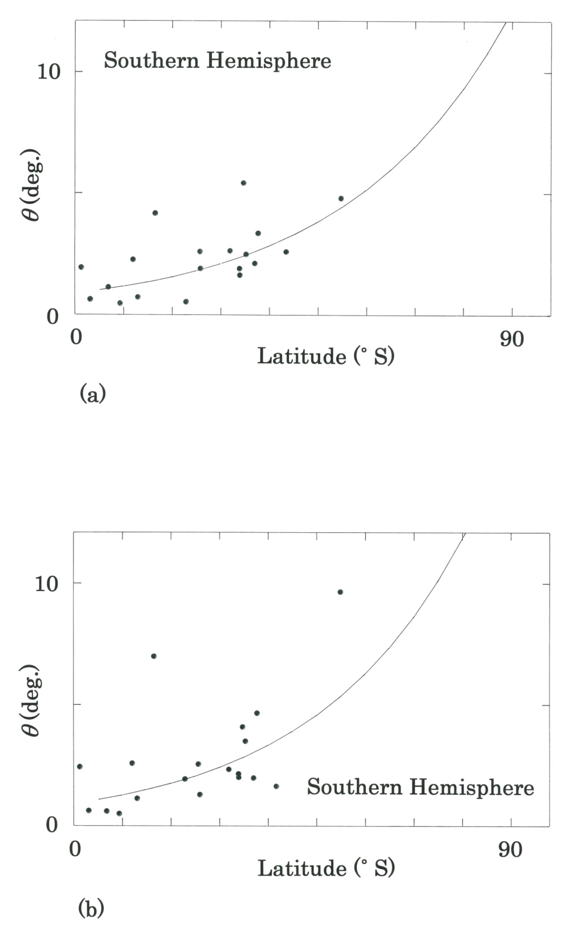
From the results plotted on Figure 3 and from those listed in Table 3 and Table 4, it is found that although the effect due to the warming is not as strong as in the northern counterpart the conclusion for the Northern Hemisphere is also applicable to the Southern Hemisphere. Autocorrelation between the rotation for the latter (Period II–III) and that for the former (Period I–II) has been found to be r = 0.843 and d = 1.806 > d_U = 1.13 (n = 19), but with the best exponential fit, showing contrast to the best logarithmic fit seen for the northern counterpart.

(4)

In contrast to the temperature, for the World precipitation, independently of the hemisphere as well as the period, no significant correlation has been seen in the latitudinal dependence. For the respective sequence the top-thirty rankings of the rotation angle are given in Tables S3 and S4 (Northern Hemisphere) and in Tables S5 and S6 (Southern Hemisphere) in Supplementary Material.

(5)

First, for the monthly precipitation on the Northern Hemisphere, irrespective of the period, the best fit on the rotation angle versus the latitude has been obtained for the linear regression. To be specific, (r, d) = (−0.107, 1.861) for Period I (1931–1960) to Period II (1951–1980), and (r, d) = (0.014, 2.210) for Period II (1951–1980) to Period III (1981–2010). In sharp contrast to this, autocorrelation between the rotation for the latter (Period II–III) and that for the former (Period I–II) has been found to be (r, d) = (0.666, 1.797) with the best logarithmic fit, showing moderate inertia throughout eighty years under consideration. The fact that Asswan (23°57′ N, 32°49′ E, h = 201 m) gains top score in both Tables S3 and S4 can be explained by noticing that the station which belongs with the Köppen’s climatic classification to BW [68] has little precipitation because of the extremely dry climate inherent in the Sahara Desert. Indeed, on Asswan the monthly precipitation data (mm) [66,67,68] are cited, from January to December (semicolon in the middle indicates the boundary between June and July), with (0.0, 0.0, 0.0, 0.0, 1.0, 0.0; 0.0, 0.0, 0.0, 0.0, 0.0, 0.0) for Period I (1931–1960), (0.1, 0.0, 0.1, 0.3, 0.0, 0.0; 0.0, 0.0, 0.0, 0.0, 0.0, 0.0) for Period II (1951–1980), (0.7, 0.0, 0.8, 0.4, 0.3, 0.0; 0.0, 0.0, 0.0, 0.6, 0.2, 0.1) for Period III (1981–2010). Here, one sees a series of nulls. The stations that have raised the ranking considerably (bold-faced in Table S4) are #47→#6: Kingston (17°56′ N), #76→#8: Karachi (24°54′ N), #56→#9: Athinai (37°44′ N), #78→#10: Lyon (45°43′ N), #68→#12: New Orleans (29°59′ N), #46→#13: Sofia (42°39′ N), #50→#14: Hong Kong (22°18′ N), #88→#18: Koebenhavn (55°41′ N), #52→#20: Anchorage (61°09′ N), #70→#21: Gibraltar (36°09′ N), # 58→#26: Madrid (40°24′ N), and #62→#28: Ankara (39°57′ N).

(6)

Next, for the monthly precipitation in the Southern Hemisphere, independently of the period, the best fit on the rotation angle versus the latitude has been obtained for the exponential regression, namely, (r, d) = (0.440, 2.780) for Period I (1931–1960) to Period II (1951–1980), whereas (r, d) = (0.409, 2.422) for Period II (1951–1980) to Period III (1981–2010). Autocorrelation between the rotation for the latter (Period II–III) and that for the former (Period I–II) has been found to be (r, d) = (0.289, 2.148) with the best logarithmic fit, indicating weak inertia over the eighty years. The three stations that follow raise the ranking significantly (see Tables S5 and S6): #11→#3: Canberra (35°18′ S), #12→#4: Salvador (13°01′ S), and #13→#5: Rio De Janeiro (22°55′ S).

4.2. Regional Analysis

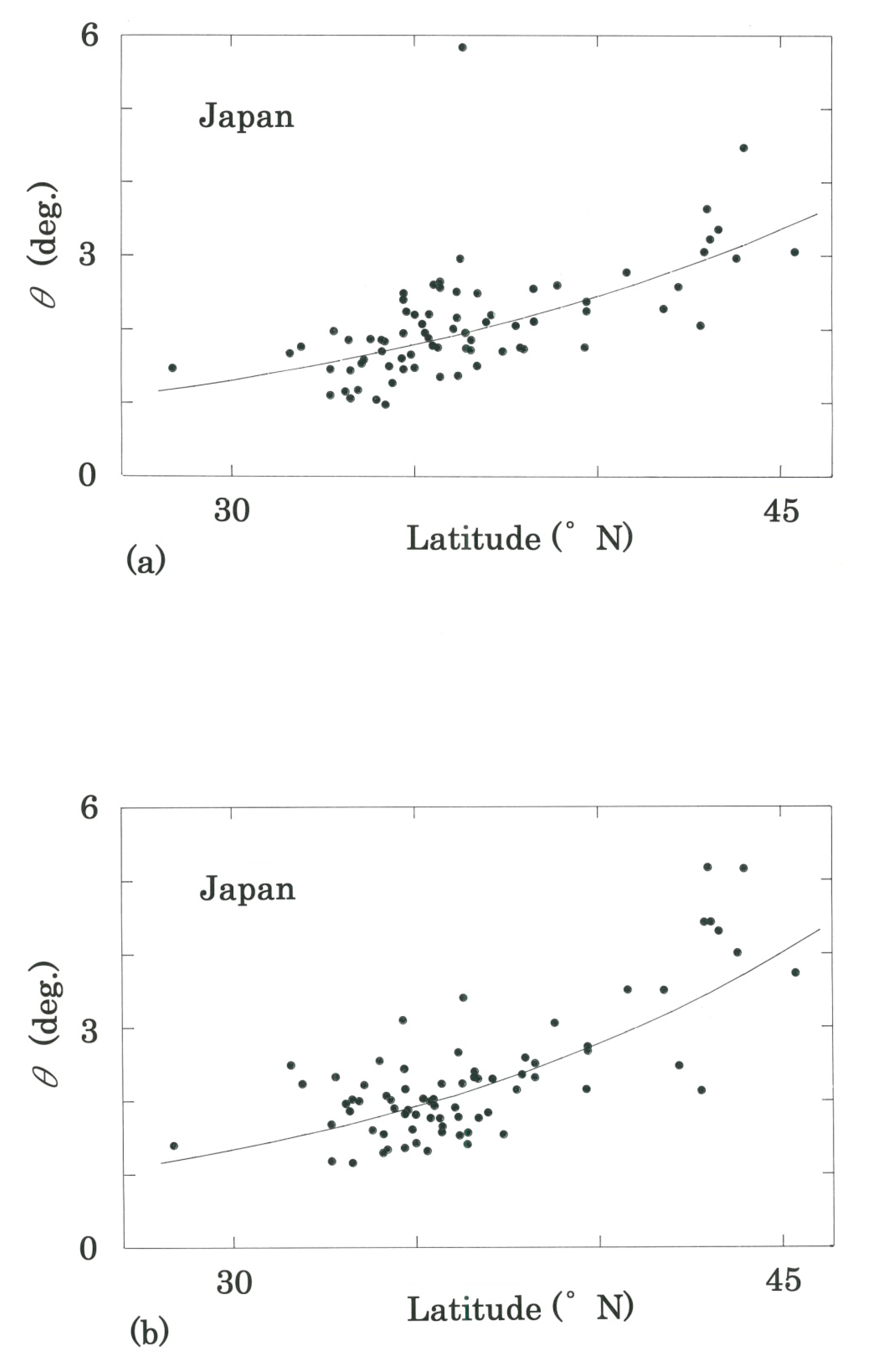
In a regional analysis, we concentrate on 75 observational stations in Japan [66,67,68], the co-ordinates of which are given in Table S7 in Supplementary Material. For monthly average temperature data, the dependence of the rotation angle on the latitude is plotted in Figure 4a for Period I (1931–1960) to Period II (1951–1980) and in Figure 4b for Period II (1951–1980) to Period III (1981–2010). The top-twenty rankings of the rotation angle are given, respectively, in

Table 5. Top-twenty Japanese stations in the rotation angle of the monthly distributions of temperatures from Period I (1931–1960) to II (1951–1980).

and

Table 6. Top-twenty Japanese stations in the rotation angle of the monthly distributions of temperatures from Period II (1951–1980) to III (1981–2010).

. In addition to the latitudinal dependence, for the respective sequence, the longitudinal dependence of the angle is shown in Figure 5. Moreover, to discuss the snow-albedo effect in more detail, data of snow cover are given in Figure 6 as a function of the latitude. Lastly, top-twenty Japanese stations in the rotation angle of the monthly distributions of precipitations are listed in Tables S8 and S9 in Supplementary Material. With these results, one can conclude as follows:

(1)

In Figure 4a, which plots the rotation between Period I (1931–1960) and Period II (1951–1980), in the same way as its global counterparts (Figure 2a and Figure 3a) the best fit has been found to be exponential but with r = 0.642 and d = 1.867 > d_U = 1.50 (n =75). (cf. for the linear regression of Equation (8), r = 0.597 with d = 1.876.) It can be seen from Table 5 that the top-twenty ranking is occupied by the stations of the northern areas being located on Hokkaido (#2 - #8, and #14) and the Tohoku Region (#10, #13, and #15), as well as the Nagano Prefecture (#1, #9, and #18). Moreover, it is interesting to note that besides #4: Sapporo and #15: Sendai there are two megacities, #11: Tokyo and #19: Osaka, on that ranking.

(2)

In Figure 4b, which plots the rotation between Period II (1951–1980) and Period III (1981–2010), the best regression has again been exponential but with r = 0.723 and d = 1.616 > d_U = 1.50 (n = 75). (Note that, although, for the linear regression of Equation (8), we have obtained r = 0.752, the ratio d = 1.461 has been below d_U.) The stations that have raised ranking substantially (see boldfaces in Table 6) are #22→#9: Hakodate (41′49′ N), #57→#11: Okayama (34°40′ N), #21→#13: Morioka (39°42′ N), #23→#14: Akita (39°43′ N), #51→#16: Aikawa (38°02′ N), #74→#17: Shimonoseki (33°57′ N), #29→#18: Yamagata (38°15′ N), and #55→#19: Kagoshima (31°33′ N). It should be noted in Table 6 that the occupation by the three cold districts remains high, namely, there are nine stations in Hokkaido (#1–#7, #9, and #20), five stations in the Tohoku Region (#8, #12 - #14, and #18), and one station in the Nagano Prefecture (#10). Autocorrelation between the rotation for the latter (Period II–III) and that for the former (Period I–II) has been found to be r = 0.687 and d = 1.322 < d_L = 1.45 for n = 75 with the best linear fit.

(3)

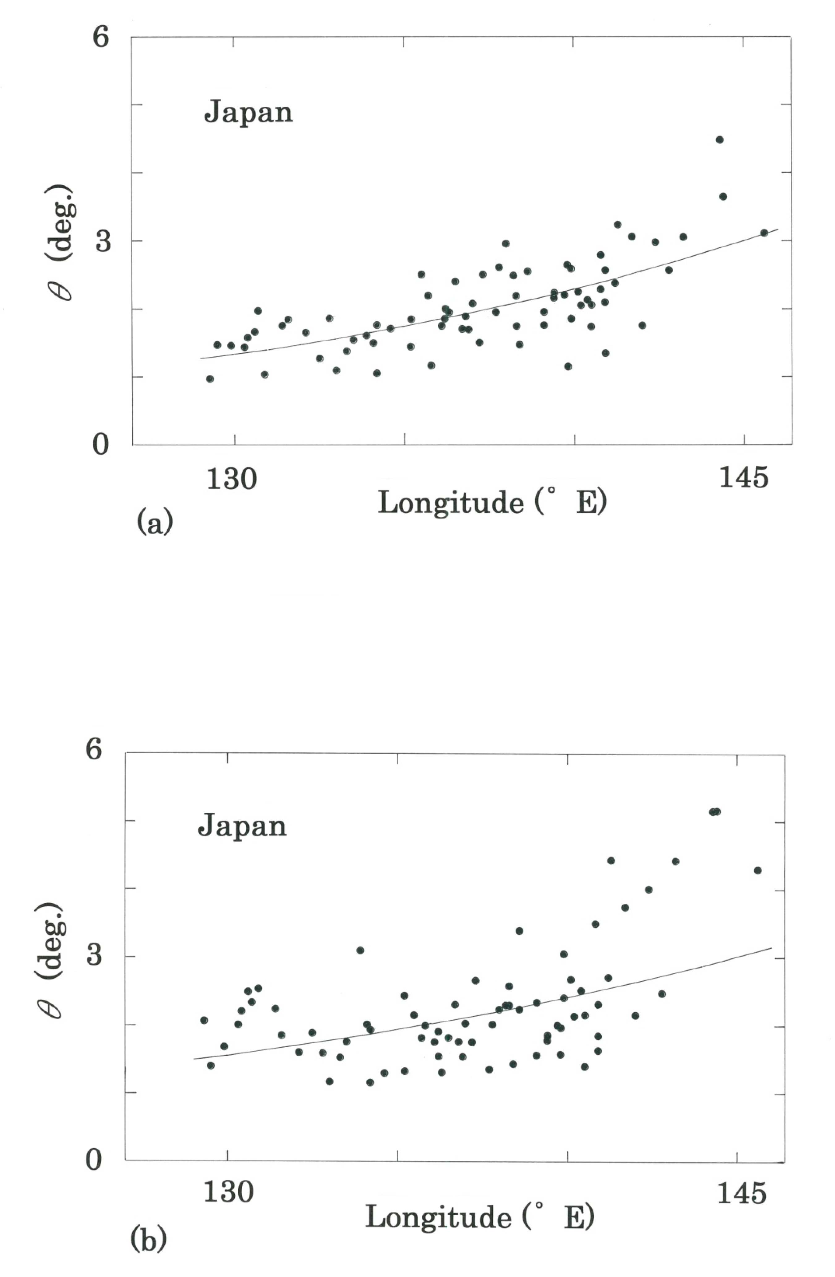
To reinforce the conclusion above, the dependence of the rotation angle on the longitude is shown in Figure 5a for Period I (1931–1960) to Period II (1951–1980) and Figure 5b for Period II (1951–1980) to Period III (1981–2010). For both cases the best fit has been made for the exponential function: (r, d) = (0.648, 1.930) for Figure 5a, whereas (r, d) = (0.511, 1.120) for Figure 5b. The results are consistent with the fact that the latitudes of the Japanese stations depend exponentially on their longitudes, with (r, d) = (0.831, 1.402). In a comparison between Figure 5a, b, it should be noted that, unlike the observation on the comparison between Figure 4a, b, no increase of the gradient of the regressive curve is seen in the longitudinal dependence of the angle, concluding that from both plots, effects due to the snow/ice-albedo feedback are not detectable longitudinally.

(4)

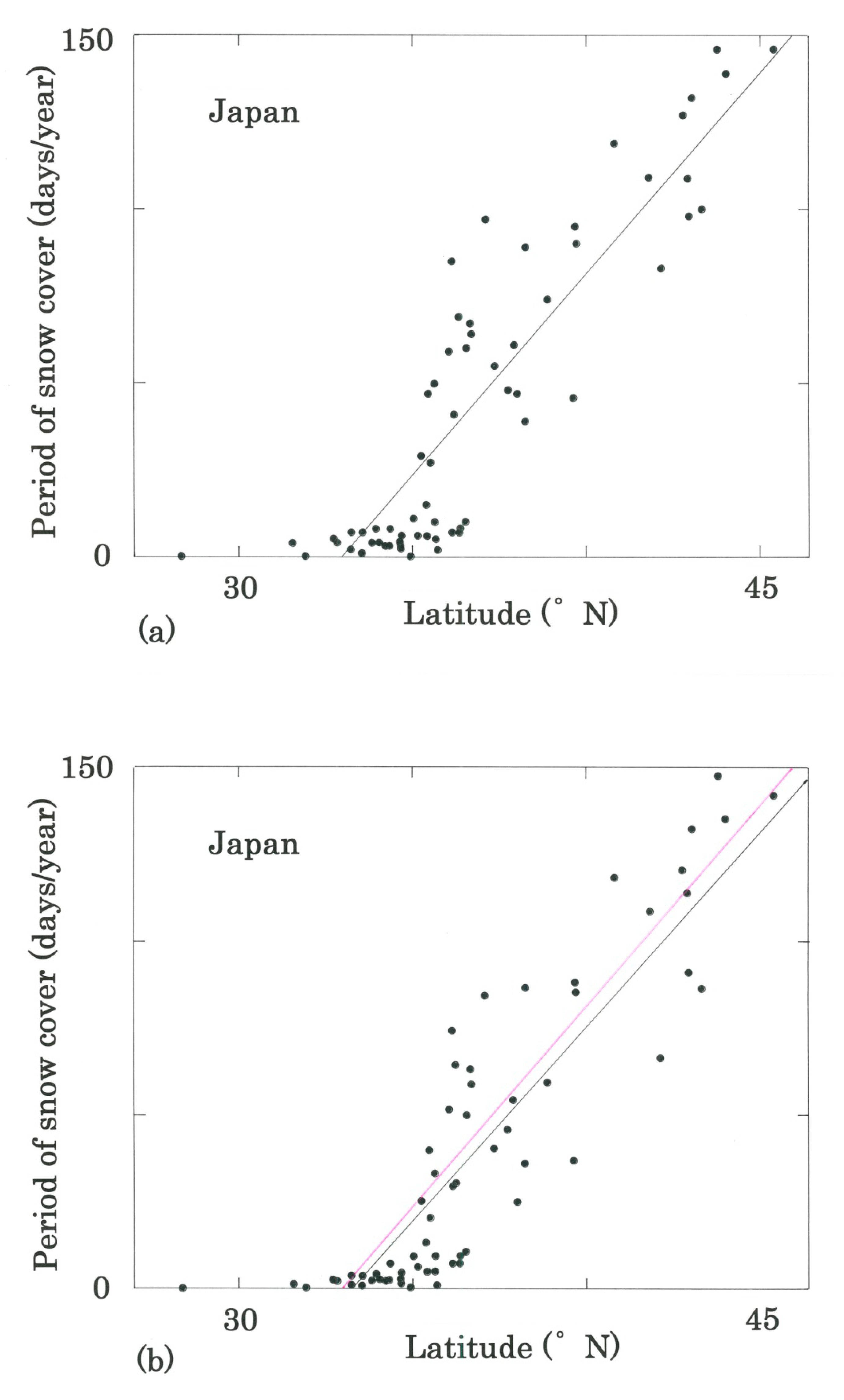
Concerning the period of snow cover, higher correlation has been found on the latitude. Specifically, for Figure 6a, r = 0.890 (linear fit) with d = 1.634 > d_U = 1.47 (n = 65), and for Figure 6b, r = 0.888 (linear fit) with d = 1.758 > d_U = 1.47 (n = 65). A comparison between the result of Figure 6a and that of Figure 6b shows that in Japan the latitudinal dependence of snow cover decreases gradually. Note that the gradient of the regressive line on Figure 6b is 96% that on Figure 6a.

(5)

Irrespective of the period, for the precipitation data, the latitudinal dependence of the angle has been shown to obey the linear model: for the results between Period I (1931–1960) and Period II (1951–1980), r = 0.399 with d = 1.671 > d_U = 1.50 (n = 75), while for those between Period II (1951–1980) and Period III (1981–2010), r = 0.120 with d = 1.920 > d_U = 1.50 (n = 75). The top-twenty ranking is given, respectively, in Table S8 and Table S9 in Supplementary Material. In Table S9 the stations that have raised ranking remarkably are #23→#3: Nemuro (43°20′ N), #39→#6: Murotomisaki (33°15′ N), #31→#8: Matsumoto (36°15′ N), #67→#12: Ida (35°31′ N), #48→#14: Tsu (34°44′ N), #45→#15: Kobe (34°42′ N), #33→#16: Aomori (40° 49′ N), and #60→#19: Naze (28°23′ N). Autocorrelation between the sequence has also been found to obey the linear regression: r = 0.392 with 4 - d = 1.755 > d_U = 1.50 (n = 75).

4.3. Toward Detecting Synchronization

The global change of climate may give rise to the so-called teleconnection [75,76,77,78], the unexpected synchronization of meteorological data among faraway spots on Earth. Here, in contrast to the traditional teleconnection studies in which either the phase synchronization or the synchronized chaos was of main concern, we regard the two spots as climatically synchronous if the cross angle between the two monthly mean vectors over the three decades decreases monotonically over the entire period, I to III. Of the ₉₇C₂ (= 4656) combinations possible on the Northern Hemisphere, it has been found that the monthly average temperature patterns on spots in the northern district of Japan and those in North America as well as in Eastern Europe exhibit a synchronous behavior. Main results are summarized in

Table 7. The sequence of the cross angle of the monthly distributions of temperatures between three North-American and five Japanese stations.

and

Table 8. The sequence of the cross angle of the monthly distributions of temperatures between three East-European and the five Japanese stations.

. Here, five Japanese stations dispersed in Table S1 in Supplementary Material are extracted, specifically, #35: Sapporo (43°04′ N, 141°20′ E), #59: Tokyo (35°41′ N, 139°46′ E), #60: Osaka (34°41′ N, 135°31′ E), #63: Fukuoka (33°35′ N, 130°23′ E), and #72: Naze (28°23′ N, 129°30′ E). For instance, for Sapporo and Chicago the computational details of Equations (3)–(7) are given in Supplementary Material. In Table 7 and Table 8, we remark as follows:

(1)

First, the complete sequences of the cross angle of the monthly distributions of temperature between three North American stations (#37: Boston, #38: Chicago, and #46: Denver in Table S1) and the five Japanese stations are summarized in Table 7. It appears that synchronization arises solely at Sapporo, which shows striking contrast to the decreasing synchronization at the other three (Tokyo, Osaka, and Fukuoka).

(2)

Subsequently the results between three East-European stations (#20: Praha, #31: Bucuresti, and #36: Sofia in Table S1) and the five stations in Japan are given in Table 8. The tendency similar to North America (Table 7) can be seen for Eastern Europe.

(3)

Other results that seem to be worth noticing are selected in what follows (I→II→III; numerals in degrees; boldfaces highlight the difference between the beginning and the last.):

#58: Tehran (35°41′ N) - #62: Atlanta (33°39′ N): 7.4→6.2→4.0,

#61: Peshawar (34°01′ N) - #69: New Orleans (29°59′ N): 5.8→5.0→4.1,

#42: Istanbul (40°54′ N) - #59: Tokyo (35°41′ N): 6.6→6.5→5.5,

#24: Muenchen (48°21′ N) - #37: Boston (42°22′ N): 7.8→7.2→6.7,

#13: Dublin (53°26′ N) - #59: Tokyo (35°41′ N): 10.2→10.1→8.1,

#55: Dar-El-Beida (36°41′ N) - #63: Fukuoka (33°35′ N): 11.2→10.7→8.3,

#15: Irkutsk (52°16′ N) - #21: Winnipeg (49°55′ N): 14.5→13.9→9.4,

#61: Peshawar (34°01′ N) - #72: Naze (28°23′ N): 10.3→10.1→9.6,

#37: Boston (42°22′ N) - #40: Tashkent (41°20′ N): 11.2→10.0→9.8,

#38: Chicago (41°59′ N) - #39: Shenyang (41°44′ N): 16.3→14.8→12.9,

#35: Sapporo (43°04′ N) - #45: Ankara (39°57′ N): 17.3→15.9→13.7,

#19: Kiev (50°24′ N) - #37: Boston (42°22′ N): 16.2→15.0→14.5.

(4)

Of the ₁₉C₂ (=171) combinations possible on the Southern Hemisphere, a synchronous trend has been detectable as follows (I→II→III; numerals in degrees):

#07: Cape Town (33°58′ S) - #08: Sydney (33°56′ S): 3.5→2.4→2.0,

#04: Auckland (37°01′ S) - #06: Buenos Aires (34°35′ S): 6.3→6.3→5.7,

#02: Christchurch (43°29′ S) - #07: Cape Town (33°58′ S): 9.7→9.3→8.8,

#05: Canberra (35°18′ S) - #07: Cape Town (33°58′ S): 12.8→12.8→11.9,

#04: Auckland (37°01′ S) - #18: Manaus (03°08′ S): 14.3→14.2→13.9,

#02: Christchurch (43°29′ S) - #18: Manaus (03°08′ S): 21.7→21.7→21.4.

Although it appears that, at least in the six combinations, the two temperature distributions are no doubt in synchronization, the effect is found to be much weaker than that revealed in the northern counterpart.

(5)

In contrast to the ubiquitous examples of the synchronization, it is difficult to detect remarkable de-synchronization wherein two temperature patterns diverge constantly. Three rare examples are cited below (I→II→III; numerals in degrees):

#10: Koebenhavn (55°41′ N) - #38: Chicago (41°59′ N): 10.4→12.0→13.7,

#25: Wien (48°14′ N) - #38: Chicago (41°59′ N): 9.5→9.6→11.7,

#21: Winnipeg (49°55′ N) - #32: Chang-chun (43°54′ N): 9.4→11.1→11.2

5. Discussion

5.1. Global Analysis

Comparison among Figure 2 and Figure 3 indicates quantitatively that the climate change in recent years has occurred globally independently of the hemisphere, but the situation is far more apparent in the northern countries on the Northern Hemisphere than the countries on the Southern Hemisphere. It should be stressed that comparison between Figure 2a,b reproduces the conclusion of former studies that owing to the snow/ice-albedo feedback [63,79,80,81,82] the regions with the higher latitudes on the Northern Hemisphere are most susceptible of the warming [83,84]. The effect can be explained by an increasing light absorption arising from degenerating cover of snow and ice that show, in comparison with the seawater and the ground, relatively higher reflectivity (at least 85 to 90% for snow whereas 65% for ice) of sunlight [1,2,69]. There are three reasons why the warming is more intense in the Northern Hemisphere (Figure 2) than the Southern Hemisphere (Figure 3):

(1)

The emission of major greenhouse gases such as the carbon dioxide, methane, ozone, and chlorofluorocarbons (CFCs) is unevenly distributed toward the former hemisphere, particularly in the region over 30° N to 60° N where there are many industrialized countries. The emission from the latter hemisphere cannot bear comparison with this.

(2)

As is well-known the distribution of the Earth’s continents is unevenly distributed toward the Northern Hemisphere where the land area amounts to 1.0 × 10¹⁰ ha, whereas that of the Southern Hemisphere is 4.9 × 10⁹ ha. Note that the land has a specific heat lower than the sea.

(3)

In striking contrast to the critical circumstance in the Arctic, the temperature growth on the Antarctica is not as steep as the northern counterpart. The reason is that the extremely thick ice (2.0 to 2.5 km) on the Antarctic Continent is free from the exposure of the ground, making ineffective the positive feedback due to the reduced albedo (i.e., the enhanced absorption) of the surface. Note again that the optical reflectivity for snow is at least 85% to 90%.

5.2. Regional Analysis

It should be emphasized that comparison between Figure 4a,b reproduces the conclusion of the global analysis, i.e., owing to the positive feedback due to the decreased albedo the cold districts with relatively high latitude in Japan are more susceptive of the global warming. Again, the effect can be attributed to an increasing light absorption arising from degenerating cover of snow that shows high reflectivity of sunlight [1,2,69]. As in Europe and in North America, Japan has often been hit by the subsequent record-breaking heat waves. Anomalous weather phenomena such as a “tropical night,” a night when the temperature does not fall below 25 °C, have become too frequent to make the headlines on newspapers. To declare a state of emergency on spots where the temperature exceeds 35 °C, besides a conventional “tropical day” on which the temperature is 30 °C or above, the Japan Meteorological Agency invented a “day of intense heat.” In addition to the intensifying strength of the chronic heat wave in the midsummer, to date there have been reports of disasters in connection with the climate crisis:

(1)

A recent report of numerical simulations by the Okhotsk Sea Ice Museum of Hokkaido [85] has predicted that in the near future there will be no sea ice drifting from a north region of the Sea of Okhotsk to the northern coast of Hokkaido, the northernmost island of Japan. The sea ice is produced in the sea of northeastern area of Sakhalin, and the south drift is caused either by the East Sakhalin Current or by an Okhotsk anticyclone that produces an air mass [86,87]. According to the report [84] the temperature around the northern area of the Sea has risen two degrees over the last fifty years, the increment of which amounts to the three times larger than the world average. Eventually, the rise in temperature has resulted in the 30% shrinkage of the ice area over the entire Sea. It should be noted here that the freezing temperature of the sea ice is −1.8 °C [88]. Because the flow in the vicinity of the southern border of the sea ice is much susceptive of the warming, one can regard the shrinkage as a high-sensitivity sensor for the global warming. Indeed, the moving average of the temperatures on Abashiri (see Rank #2 in Table 5 and Table 6), a spot on the coastland of the Sea, versus the sea-ice force off the coast of the spot has demonstrated the negative correlation over the last thirty years [89].

(2)

Comparison between the result of Figure 6a and that of Figure 6b reveals that in Japan both the period and the latitudinal dependence of snow cover decrease gradually. Specifically, the regression lines on the plots can be written as

y = 11.59 x − 382.3   for Figure 6a

y = 11.17 x − 371.4   for Figure 6b

where x and y represent the latitude (° N) and the period of snow cover (days/year), respectively. Here it should be highlighted again that the coefficient of regression on the latter is 96% that on the former, demonstrating the influence due to the warming. Moreover, a comparison between the two plots shows that on the spot of 45° N the period of snow cover shortens for eight days in Figure 6b. Indeed, every year, ski resorts in Japan are hit by the snow shortage. Furthermore, the quality of their snow is degrading. To discuss this concern, we note that a pattern of atmospheric pressure in which the high-pressure area lies to the west and the low-pressure area to the east is characteristic of winter of the Japanese Islands. The physical mechanism of the pressure configuration can be explained as follows: First, because of the radiative cooling, temperatures in winter fall substantially on the inland areas of Siberia and China. Second, the enhanced density of the cooled air generates a descending air current, which is responsible for the emergence of the high pressure in the west of Hokkaido. Third, collision of two air masses coming from the North Pole and from the equator produces a large-scale stable vortex in the vicinity of the Kuriles and the southern area of the Kamchatka Peninsula; eventually the vortex is responsible for observing the low pressure in the east of Hokkaido. The warming as shown especially in the relatively high latitudes of the Northern Hemisphere (see Figure 2) is responsible for reducing the radiative cooling, i.e., reducing the strength of a seasonal wind from the Eurasian Continent to Hokkaido. In Table 2, one can confirm the reason, for instance, on Rank #13: Vladivostok (43°07′ N), #14: Irkutsk (52°16′ N), and #23: Chang-chun (43°54′ N). In response to the shrinkage of the Siberian cold mass moving southeast from the Maritime Territory (Primorsky Kray) of Russia to the Hidaka mountains, the world-renowned powdery snow on resorts in Hokkaido threatens to be in a critical condition.

5.3. Toward Detecting Synchronization

Of the combinations possible on the Northern Hemisphere, it has been found that the monthly averaged temperature patterns on spots in the northern district of Japan and those in North America (Table 7) as well as in Eastern Europe (Table 8) exhibit a synchronous behavior. First of all, it should be noted that Japan consists of the four major islands, i.e., Hokkaido, Honshu, Shikoku, and Kyushu. Of these, Hokkaido is separate from Honshu via the Blakiston’s line on the midst of the Tsugaru Strait, across which the climate as well as the ecosystem change substantially. The line was found by a British zoologist and soldier, Thomas Wright Blakiston (1832–1891), who determined a zoogeographic border between the northern Siberian and the southern Manchurian subzone. While the line gives the northern limit of Asiatic black bears, Japanese monkeys, and Japanese squirrels, it gives the southern limit of brown bears, Asiatic pikas, and Eurasian striped squirrels. Specifically, with the Köppen’s climatic classification, the former island (Hokkaido) belongs to Dfa whereas the latter three (Honshu, Shikoku, and Kyushu) belong to Cfa. Consequently, in both vegetation and soil, there are qualitative differences between the two regions across the strait. First, in Hokkaido there is no long spell of rainy weather in early summer, but in winter the surface is covered with snow. Second, the northernmost island is seldom visited by a typhoon because, as it propagates northward, the tropical cyclone generated in the vicinity of the Philippine Islands is converted gradually to an extratropical storm with its energy much more dispersed than the cyclone. With respect to features peculiar to the land, Sapporo, being located in Hokkaido, and the stations in North America and Europe share something in common in that they have a cool temperature climate. Here, we note that the Köppen’s climatic classifications are Dfa for Boston, Chicago, and Bucuresti, with Cfb for Praha and Sofia and BSk for Denver.

6. Conclusions

For 116 observational stations in the world, sequential variations of the monthly distributions of meteorological data have been analyzed. For specific monthly data, precipitations as well as temperatures have been chosen, both of which are averaged over thirty years. Climate change can be detected through calculating the intersecting angle between two twelve-dimensional vectors being composed with monthly mean values. To enhance the precision and to avoid the production of a number of tie data, additional 21 components consisting of eleven first-order and ten second-order differences have been incorporated in each vector. With this extension, one eventually obtains the 33-dimensional vector. Subsequently the angle data for the entire stations have been analyzed statistically and been compared between the former (1931–1980) and the latter (1951–2010) period. With nonlinear as well as linear regressions, irrespective of the period and the hemisphere, the variation of the rotation angles has been found to show the exponential growth as a function of their latitudes. Furthermore, this trend has been shown to be stronger in the latter period, indicating that the snow/ice-albedo feedback gets stronger. In contrast to the World temperature, for the precipitation, no significant correlation has been found between the angle and the latitude. In order to examine the albedo feedback in more detail, a regional analysis has been carried out as well. Specifically, 75 stations in Japan, which range from 28°23′ N to 45°25′ N, have been chosen. Numerical results have shown that the warming is significant even for the relatively narrow range (19%) of the hemisphere. Finally, a synchronization of the monthly patterns of temperatures has been given between the northern district of Japan and both North America and Eastern Europe. To the author’s knowledge, the methodology given in this paper is original and bears a comprehensive applicability also to the analysis of meteorological data other than the temperature and the precipitation. With this method, unknown synchronizations could be revealed. To conclude, the combination of vectorial and statistical analysis has allowed one to reveal the world-scale impendence distinctly.

In an essay published in 1957 [90], Ukichiro Nakaya (1900–1962), who is known worldwide for his achievement of artificial snow, issued a warning as a precursor of global warming. Along with earlier studies, including the IPCC’s reports, and with the predictions by Earth simulators running all over the world, our results presented in this paper have demonstrated statistically that his presage was far from utterly unfounded. For global warming, we are now in a position to prepare to relieve the damage on the assumption that planet Earth will continue to become warmer, slowly but surely.

References

- Weart, S.R. The Discovery of Global Warming; Harvard University Press: Cambridge, MA, USA, 2008. [Google Scholar]
- Stocker, T.F.; Qin, D.; Plattner, G.-K.; Tignor, M.M.B.; Allen, S.K.; Boschung, J.; Nauels, A.; Xia, Y.; Bex, V.; Midgley, P.M. (Eds.) Climate Change 2013: The Physical Science Basis (Working Group I Contribution to the Fifth Assessment Report of the Intergovernmental Panel on Climate Change); Cambridge University Press: Cambridge, UK, 2014. [Google Scholar]
- GOSAT Project, the National Institute for Environmental Studies, Japan. A Prompt Report on the Monthly Mean Carbon-Dioxide Concentration Averaged over the Entire Atmosphere. 2016. Available online: http://www.gosat.nies.go.jp/recent-global-co2.html (accessed on 19 July 2020).
- HadCRUT4 dataset produced by the Met Office and the Climatic Research Unit at the University of East Anglia. Global Climate in Context as the World Approaches 1 °C above Pre-Industrial for the First Time; 2015. Available online: https://www.metoffice.gov.uk/research/news/2015/global-average-temperature-2015 (accessed on 19 July 2020).
- An Opinion Offered by the Medical Association of Japan. 2018. Available online: https://www.asahi.com/articles/ASLBY5FX1LBY5X1LBYULZU00H.html (accessed on 12 August 2020).
- Yamamoto, R.; Hoshiai, M. Fluctuations of the Northern Hemisphere mean surface air temperature during recent 100 years estimated by optimum interpolation. J. Meteor. Soc. Jpn. 1980, 58, 187–193. [Google Scholar] [CrossRef] [Green Version]
- Hansen, J.E.; Johnson, D.; Lacis, A.; Lebedeff, S.; Lee, P.; Rind, D.; Russell, G. Climatic impact of increasing atmospheric carbon dioxide. Science 1981, 213, 957–966. [Google Scholar] [CrossRef] [Green Version]
- Jones, P.D.; Wigley, T.M.L.; Kelly, P.M. Variations in surface air temperatures: Part 1. Northern Hemisphere, 1881–1980. Mon. Weather Rev. 1982, 110, 59–72. [Google Scholar] [CrossRef] [Green Version]
- Jones, P.D.; Kelly, P.M. The spatial and temporal characteristics of Northern Hemisphere surface air temperature variations. J. Climatol. 1983, 3, 243–252. [Google Scholar] [CrossRef]
- Jones, P.D.; Raper, S.C.B.; Bradley, R.S.; Diaz, H.F.; Kelly, P.M.; Wigley, T.M.L. Northern hemisphere surface air temperature variations: 1851–1984. J. Clim. Appl. Meteor. 1986, 25, 161–179. [Google Scholar] [CrossRef] [Green Version]
- Hansen, J.E.; Lebedeff, S. Global trends of measured surface air temperature. J. Geophys. Res. 1987, 92, 13345–13372. [Google Scholar] [CrossRef] [Green Version]
- Lacis, A.A.; Wuebbles, D.J.; Logan, J.A. Radiative forcing of climate by changes in the vertical distribution of ozone. J. Geophys. Res. 1990, 95, 9971–9981. [Google Scholar] [CrossRef]
- Bloomfield, P. Trends in global temperature. Clim. Chang. 1992, 21, 1–16. [Google Scholar] [CrossRef]
- Bloomfield, P.; Nychka, D.W. Climate spectra and detecting climate change. Clim. Chang. 1992, 21, 275–287. [Google Scholar] [CrossRef]
- Wallace, J.M.; Zhang, Y.; Renwick, J.A. Dynamic contribution to hemispheric mean temperature trends. Science 1995, 270, 780–783. [Google Scholar] [CrossRef]
- Hansen, J.; Sato, M.; Glascoe, J.; Ruedy, R. A common-sense climate index: Is climate changing noticeably? Proc. Natl. Acad. Sci. USA 1998, 95, 4113–4120. [Google Scholar] [CrossRef] [Green Version]
- Jones, P.D.; New, M.; Parker, D.E.; Martin, S.; Rigor, I.G. Surface air temperature and its changes over the past 150 years. Rev. Geophys. 1999, 37, 173–199. [Google Scholar] [CrossRef]
- Gaffen, D.J.; Ross, R.J. Climatology and trends of U.S. surface humidity and temperature. J. Clim. 1999, 12, 811–828. [Google Scholar] [CrossRef]
- New, M.; Hulme, M.; Jones, P. Representing twentieth-century space-time climate variability. Part I: Development of a 1961-90 mean monthly terrestrial climatology. J. Clim. 1999, 12, 829–856. [Google Scholar] [CrossRef]
- Berntsen, T.K.; Myhre, G.; Stordal, F.; Isaksen, I.S.A. Time evolution of tropospheric ozone and its radiative forcing. J. Geophys. Res. 2000, 105, 8915–8930. [Google Scholar] [CrossRef]
- Deser, C.; Walsh, J.E.; Timlin, M.S. Arctic sea ice variability in the context of recent atmospheric circulation trends. J. Clim. 2000, 13, 617–633. [Google Scholar] [CrossRef]
- Lelieveld, J.; Dentener, F.J. What controls tropospheric ozone? J. Geophys. Res. 2000, 105, 3531–3551. [Google Scholar] [CrossRef]
- New, M.; Hulme, M.; Jones, P. Representing twentieth-century space-time climate variability. Part II: Development of 1901-96 monthly grids of terrestrial surface climate. J. Clim. 2000, 13, 2217–2238. [Google Scholar] [CrossRef]
- Zhang, X.; Vincent, L.A.; Hogg, W.D.; Niitsoo, A. Temperature and precipitation trends in Canada during the 20th century. Atmos.-Ocean. 2000, 38, 395–429. [Google Scholar] [CrossRef]
- Hansen, J.E.; Ruedy, R.; Sato, M.; Imhoff, M.; Lawrence, W.; Easterling, D.; Peterson, T.; Karl, T. A closer look at United States and global surface temperature change. J. Geophys. Res. 2001, 106, 23947–23963. [Google Scholar] [CrossRef] [Green Version]
- Hansen, J.E.; Sato, M. Trends of measured climate forcing agents. Proc. Natl. Acad. Sci. USA 2001, 98, 14778–14783. [Google Scholar] [CrossRef] [Green Version]
- Wang, J.X.L.; Gaffen, D.J. Late-twentieth-century climatology and trends of surface humidity and temperature in China. J. Clim. 2001, 14, 2833–2845. [Google Scholar] [CrossRef]
- Thompson, D.; Solomon, S. Interpretation of recent Southern Hemisphere climate change. Science 2002, 296, 895–899. [Google Scholar] [CrossRef] [Green Version]
- Jones, P.D.; Moberg, A. Hemispheric and large-scale surface air temperature variations: An extensive revision and an update to 2001. J. Clim. 2003, 16, 206–223. [Google Scholar] [CrossRef] [Green Version]
- Philipona, R.; Duerr, B. Greenhouse forcing outweighs decreasing solar radiation driving rapid temperature rise over land. Geophys. Res. Lett. 2004, 31. [Google Scholar] [CrossRef]
- Luterbacher, J.; Dietrich, D.; Xoplaki, E.; Grosjean, M.; Wanner, H. European seasonal and annual temperature variability, trends, and extremes since 1500. Science 2004, 303, 1499–1503. [Google Scholar] [CrossRef] [Green Version]
- Meehl, G.A.; Tebaldi, C. More intense, more frequent, and longer lasting heat waves in the 21st century. Science 2004, 305, 994–997. [Google Scholar] [CrossRef] [Green Version]
- Philipona, R.; Duerr, B.; Ohmura, A.; Ruckstuhl, C. Anthropogenic greenhouse forcing and strong water vapor feedback increase temperature in Europe. Geophys. Res. Lett. 2005, 32, L19809. [Google Scholar] [CrossRef]
- Tebaldi, C.; Hayhoe, K.; Arblaster, J.M.; Meehl, G.A. Going to the extremes: An intercomparison of model-simulated historical and future changes in extreme events. Clim. Chang. 2006, 79, 185–211. [Google Scholar] [CrossRef]
- Seidel, D.J.; Randel, W.J. Recent widening of the tropical belt: Evidence from tropopause observations. J. Geophys. Res. 2007, 112, D20113. [Google Scholar] [CrossRef] [Green Version]
- Vincent, L.A.; van Wijngaarden, W.A.; Hopkinson, R. Surface temperature and humidity trends in Canada for 1953–2005. J. Clim. 2007, 20, 5100–5113. [Google Scholar] [CrossRef]
- Thompson, D.W.J.; Kennedy, J.J.; Wallace, J.M.; Jones, P.D. A large discontinuity in the mid-twentieth century observed global-mean surface temperature. Nature 2008, 453, 646–649. [Google Scholar] [CrossRef] [PubMed]
- Portmann, R.W.; Solomon, S.; Hegerl, G.C. Spatial and seasonal patterns in climate change, temperatures, and precipitation across the United States. Proc. Natl. Acad. Sci. USA 2009, 106, 7324–7329. [Google Scholar] [CrossRef] [Green Version]
- Swanson, K.L.; Sugihara, G.; Tsonis, A.A. Long-term natural variability and 20th century climate change. Proc. Natl. Acad. Sci. USA 2009, 106, 16120–16130. [Google Scholar] [CrossRef] [Green Version]
- Morak, S.; Hegerl, G.C.; Kenyon, J. Detectable regional changes in the number of warm nights. Geophys. Res. Lett. 2011, 38, L17703. [Google Scholar] [CrossRef] [Green Version]
- Arblaste, J.M.; Meehl, G.A.; Karoly, D.J. Future climate change in the Southern Hemisphere: Competing effects of ozone and greenhouse gases. Geophys. Res. Lett. 2011, 38, L02701. [Google Scholar] [CrossRef]
- Francis, J.A.; Vavrus, S.J. Evidence linking Arctic amplification to extreme weather in mid-latitudes. Geophys. Res. Lett. 2012, 39, L06801. [Google Scholar] [CrossRef]
- Franzke, C. On the statistical significance of surface air temperature trends in the Eurasian Arctic region. Geophys. Res. Lett. 2012, 39, L23705. [Google Scholar] [CrossRef] [Green Version]
- Hansen, J.; Sato, M.; Ruedy, R. Perception of climate change. Proc. Natl. Acad. Sci. USA 2012, 109, E2415–E2423. [Google Scholar] [CrossRef] [Green Version]
- Jones, P.D.; Lister, D.H.; Osborn, T.J.; Harpham, C.; Salmon, M.; Morice, C.P. Hemispheric and large-scale land surface air temperature variations: An extensive revision and an update to 2010. J. Geophys. Res. 2012, 117, D05127. [Google Scholar] [CrossRef] [Green Version]
- Mika, J. Changes in weather and climate extremes: Phenomenology and empirical approaches. Clim. Chang. 2013, 121, 15–26. [Google Scholar] [CrossRef]
- Ji, F.; Wu, Z.; Huang, J.; Chassignet, E.P. Evolution of land surface air temperature trend. Nat. Clim. Chang. 2014, 4, 462–466. [Google Scholar] [CrossRef]
- Screen, J.A. Arctic amplification decreases temperature variance in northern mid- to high-latitudes. Nat. Clim. Chang. 2014, 4, 577–582. [Google Scholar] [CrossRef] [Green Version]
- Robeson, S.M.; Willmott, C.J.; Jones, P.D. Trends in hemispheric warm and cold anomalies. Geophys. Res. Lett. 2014, 41, 9065–9071. [Google Scholar] [CrossRef]
- Ganopolski, A.; Rahmstorf, S. Abrupt glacial climate changes due to stochastic resonance. Phys. Rev. Lett. 2002, 88, 038501. [Google Scholar] [CrossRef] [Green Version]
- Király, A.; Jánosi, I.M. Stochastic modeling of daily temperature fluctuations. Phys. Rev. E 2002, 65, 051102. [Google Scholar] [CrossRef] [PubMed]
- Lind, P.G.; Mora, A.; Gallas, J.A.C.; Haase, M. Reducing stochasticity in the North Atlantic Oscillation index with coupled Langevin equations. Phys. Rev. E 2005, 72, 056706. [Google Scholar] [CrossRef]
- Redner, S.; Petersen, M.R. Role of global warming on the statistics of record-breaking temperatures. Phys. Rev. E 2006, 74, 061114. [Google Scholar] [CrossRef] [Green Version]
- Verdes, P.F. Global warming is driven by anthropogenic emissions: A time series analysis approach. Phys. Rev. Lett. 2007, 99, 048501. [Google Scholar] [CrossRef]
- Adair, R.K. Stochastic contribution to global temperature changes. Phys. Rev. Lett. 2008, 100, 148501. [Google Scholar] [CrossRef]
- Newman, W.I.; Malamud, B.D.; Turcotte, D.L. Statistical properties of record-breaking temperatures. Phys. Rev. E 2010, 82, 066111. [Google Scholar] [CrossRef] [PubMed] [Green Version]
- Tamazian, A.; Ludescher, J.; Bunde, A. Significance of trends in long-term correlated records. Phys. Rev. E 2015, 91, 032806. [Google Scholar] [CrossRef] [PubMed] [Green Version]
- Drótos, G.; Bódai, T.; Tél, T. Quantifying nonergodicity in nonautonomous dissipative dynamical systems: An application to climate change. Phys. Rev. E 2016, 94, 022214. [Google Scholar] [CrossRef] [Green Version]
- Huang, X.; Hassani, H.; Ghodsi, M.; Mukherjee, Z.; Gupta, R. Do trend extraction approaches affect causality detection in climate change studies? Phys. A 2017, 469, 604–624. [Google Scholar] [CrossRef] [Green Version]
- Zhang, F.; Yang, P.; Fraedrich, K.; Zhou, X.; Wang, G. Reconstruction of driving forces from nonstationary time series including stationary regions and application to climate change. Phys. A 2017, 473, 337–343. [Google Scholar] [CrossRef]
- Matcharashvili, T.; Zhukova, N.; Chelidze, T.; Founda, D.; Gerasopoulos, E. Analysis of long-term variation of the annual number of warmer and colder days using Mahalanobis distance metrics: A case study for Athens. Phys. A 2017, 487, 22–31. [Google Scholar] [CrossRef]
- Popović, P.; Cael, B.B.; Silber, M.; Abbot, D.S. Simple rules govern the patterns of Arctic sea ice melt ponds. Phys. Rev. Lett. 2018, 120, 148701. [Google Scholar] [CrossRef] [PubMed] [Green Version]
- Moon, W.; Agarwal, S.; Wettlaufer, J.S. Intrinsic pink-noise multidecadal global climate dynamics mode. Phys. Rev. Lett. 2018, 121, 108701. [Google Scholar] [CrossRef] [Green Version]
- Hassani, H.; Silva, E.S.; Gupta, R.; Das, S. Predicting global temperature anomaly: A definitive investigation using an ensemble of twelve competing forecasting models. Phys. A 2018, 509, 121–139. [Google Scholar] [CrossRef]
- Wang, C.; Wang, Z.-H.; Sun, L. Early-warning signals for critical temperature transitions. Geophys. Res. Lett. 2020, 47, e2020GL088503. [Google Scholar] [CrossRef]
- The National Astronomical Observatory, Japan (Ed.) Chronological Scientific Tables; Maruzen: Tokyo, Japan, 1985; Volume 59. [Google Scholar]
- The National Astronomical Observatory, Japan (Ed.) Chronological Scientific Tables; Maruzen: Tokyo, Japan, 1992; Volume 66. [Google Scholar]
- The National Astronomical Observatory, Japan (Ed.) Chronological Scientific Tables; Maruzen: Tokyo, Japan, 2017; Volume 91. [Google Scholar]
- Wadhams, P. A Farewell to Ice: A Report from the Arctic; Penguin Books: London, UK, 2016. [Google Scholar]
- von Storch, H.; Zwiers, F.W. Statistical Analysis in Climate Research; Cambridge University Press: Cambridge, UK, 2000. [Google Scholar]
- von Storch, H.; Navarra, A. (Eds.) Analysis of Climate Variability: Applications of Statistical Techniques, 2nd ed.; Springer: Berlin, Germany, 2010. [Google Scholar]
- Chatterjee, S.; Hadi, A.S. Regression Analysis by Example, 5th ed.; Wiley: Hoboken, NJ, USA, 2012. [Google Scholar]
- Seber, G.A.F.; Wild, C.J. Nonlinear Regression; Wiley: Hoboken, NJ, USA, 2003. [Google Scholar]
- Wang, C.; Wang, Z.-H.; Li, Q. Emergence of urban clustering among U.S. cities under environmental stressors. Sustain. Cities Soc. 2020, 63, 102481. [Google Scholar] [CrossRef]
- Duane, G.S. Synchronized chaos in extended systems and meteorological teleconnections. Phys. Rev. E 1997, 56, 6475. [Google Scholar] [CrossRef]
- Rybski, D.; Havlin, S.; Bunde, A. Phase synchronization in temperature and precipitation records. Phys. A 2003, 320, 601–610. [Google Scholar] [CrossRef] [Green Version]
- Castrejón-Pita, A.A.; Read, P.L. Synchronization in a pair of thermally coupled rotating baroclinic annuli: Understanding atmospheric teleconnections in the laboratory. Phys. Rev. Lett. 2010, 104, 204501. [Google Scholar] [CrossRef]
- Zhou, D.; Gozolchiani, A.; Ashkenazy, Y.; Havlin, S. Teleconnection paths via climate network direct link detection. Phys. Rev. Lett. 2015, 115, 268501. [Google Scholar] [CrossRef] [Green Version]
- Yizhaq, H.; Ashkenazy, Y. Why do active and stabilized dunes coexist under the same climatic conditions? Phys. Rev. Lett. 2007, 98, 188001. [Google Scholar] [CrossRef] [PubMed] [Green Version]
- Kutschan, B.; Morawetz, K.; Gemming, S. Modeling the morphogenesis of brine channels in sea ice. Phys. Rev. E 2010, 81, 036106. [Google Scholar] [CrossRef] [Green Version]
- Alberti, T.; Primavera, L.; Vecchio, A.; Lepreti, F.; Carbone, V. Spatial interactions in a modified daisyworld model: Heat diffusivity and greenhouse effects. Phys. Rev. E 2015, 92, 052717. [Google Scholar] [CrossRef]
- Lucarini, V.; Bódai, T. Transitions across melancholia states in a climate model: Reconciling the deterministic and stochastic points of view. Phys. Rev. Lett. 2019, 122, 158701. [Google Scholar] [CrossRef] [Green Version]
- Berger, J.J. Climate Peril; Northbrae: Berkeley, CA, USA, 2014. [Google Scholar]
- Welch, C.; Orlinsky, K. The threat below. Natl. Geogr. 2019, 9, 74–99. [Google Scholar]
- The Ministry of the Environment, Japan. Vanishing Floating Ice: A Symptom of Warming? 2016. Available online: https://www.youtube.com/watch?v=MuSgY5G-64I (accessed on 19 July 2020).
- Kimura, N.; Wakatsuchi, M. Processes controlling the advance and retreat of sea ice in the Sea of Okhotsk. J. Geophys. Res. 1999, 104, 11137–11150. [Google Scholar] [CrossRef]
- Kimura, N.; Wakatsuchi, M. Increase and decrease of ice area in the Sea of Okhotsk: Ice production in coastal polynyas and dynamic thickening in convergence zones. J. Geophys. Res. 2004, 109, C09S03. [Google Scholar] [CrossRef] [Green Version]
- The Okhotsk Sea Ice Museum of Hokkaido. Where Does the Sea Ice Come from? 2020. Available online: http://giza-ryuhyo.com/ (accessed on 11 September 2020).
- Aota, M. A Nightmare of the Disappearance of Sea Ice. 2006. Available online: https://www.cger.nies.go.jp/publications/news/series/watch/6-6.pdf (accessed on 11 September 2020).
- Watanabe, O. (Ed.) The Alaskan Glacier: A Book of Travels by Ukichiro Nakaya; Iwanami Shoten: Tokyo, Japan, 2002. [Google Scholar]
Figure 1.
The location of 116 observational stations (pink dots) in the world. Meteorological data on the spots are used in the global analysis.
Figure 2.
Rotation angles between the monthly distributions of temperatures on the 97 Northern-Hemispheric stations versus their latitudes. (a) Rotation is considered from Period I (1931–1960) to Period II (1951–1980). The curve superimposed in the plots represents the optimal exponential regression (r = 0.738 with d = 1.788 > dU = 1.55 for n = 97). Note that the Urumchi’s angle θ = 17.80° on the top in Table 1 is truncated. (b) Rotation from Period II (1951–1980) to Period III (1981–2010). The curve in the plots represents the optimal exponential regression (r = 0.843 with d = 1.089 < dL = 1.51 for n = 97).
Figure 3.
Rotation angles between the monthly distributions of temperatures on the 19 Southern-Hemispheric stations versus their latitudes. (a) Rotation from Period I (1931–1960) to Period II (1951–1980) is calculated. The curve in the plots represents the optimal exponential regression (r = 0.605 with 4 - d = 1.172 > dU = 1.13 for n = 19). (b) Rotation from Period II (1951–1980) to Period III (1981–2010). The curve in the plots represents the optimal exponential regression (r = 0.598 with 4 − d = 1.787 > dU = 1.13 for n = 19).
Figure 4.
Rotation angles between the monthly distributions of temperatures on the 75 Japanese stations versus their latitudes. (a) Rotation from Period I (1931–1960) to Period II (1951–1980) is dealt with. The curve in the plots represents the optimal exponential regression (r = 0.642 with d = 1.867 > dU = 1.50 for n = 75). (b) Rotation from Period II (1951–1980) to Period III (1981–2010). The curve in the plots represents the optimal exponential regression (r = 0.723 with d = 1.616 > dU = 1.50 for n = 75).
Figure 5.
Rotation angles between the monthly distributions of temperatures on the 75 Japanese stations versus their longitudes. (a) Rotation from Period I (1931–1960) to Period II (1951–1980) is given. The curve in the plots represents the optimal exponential regression (r = 0.648 with d = 1.930 > dU = 1.50 for n = 75). (b) Rotation from Period II (1951–1980) to Period III (1981–2010). The curve in the plots represents the optimal exponential regression (r = 0.511 with d = 1.120 < dL = 1.45 for n = 75).
Figure 6.
The period of snow cover versus the latitude. Null data are excluded from the plot. (a) In 1980. The line superimposed in the plots represents the optimal linear regression (r = 0.890 with d = 1.634 > dU = 1.47 for n = 65). (b) In 2010. The black line in the plots represents the optimal linear regression (r = 0.888 with d = 1.758 > dU = 1.47 for n = 65). The regression of (a) 1980 is superimposed with the pink line.