Urban Morphological Controls on Surface Thermal Dynamics: A Comparative Assessment of Major European Cities with a Focus on Athens, Greece

Abstract

Variations in urban form lead to the development of distinctive intra-urban surface thermal patterns. Previous assessment of the relation between urban structure and satellite-based Land Surface Temperature (LST) has generally been limited to single-city cases. Here, examining 25 European cities (June–August 2017), we estimated the statistical association between surface parameters—the impervious fraction (λ_imp), the building fraction (λ_b), and the building height (H)—and the neighborhood scale (1000 × 1000 m) LST variations, as captured by the Moderate Resolution Imaging Spectroradiometer (MODIS) sensor. Correlation analysis, multiple linear regression, and spatial regression were used. As expected, λ_imp had a consistent positive influence on LSTs. In contrast, the relation of LST with λ_b and H was generally weaker or negative in the daytime, whereas at night it shifted to a robust positive effect. In particular, daytime LSTs of densely built, high-rise European districts tended to have lower values. This was especially the case for the city of Athens, Greece, where a more focused analysis was conducted, using further surface parameters and the Local Climate Zone (LCZ) scheme. For the urban core of the city, the canyon aspect ratio H/W had a statistically significant (p <0.01) negative relationship with LST by day (Spearman’s rho = −0.68) and positive during nighttime (rho = 0.45). The prevailing intra-urban surface thermal variability in Athens was well reproduced by a 5-day numerical experiment using the meteorological Weather Research and Forecasting Model (WRF) model and a modified urban parameterization scheme. Although the simulation resulted in some systematic errors, the overall accuracy of the model was adequate, regarding the surface temperature (RMSE = 2.4 K) and the near-surface air temperature (RMSE = 1.7 K) estimations.

1. Introduction

The urban influence on local microclimates is one of the most apparent human-driven modifications to the natural environment. As a result of the distinct features of the urban form and function, cities experience elevated temperatures relative to their surrounding rural areas—a phenomenon referred to as the urban heat island (UHI). The most important processes that drive urban climate effects can be summarized as follows [1]:

• High values of the building height (H) to street width (W) ratio—the canyon aspect ratio (H/W)—hinder long-wave radiative cooling [2] and reduce turbulent transport due to wind shelter.
• The thermal properties of urban materials as well as the characteristics of urban structure, lead to a stronger heat storage uptake during daytime and to a gradual heat release at night, maintaining a positive sensible heat flux [3].
• Low vegetation density is responsible for reduced latent heat flux and evapotranspiration cooling [4].
• The canyon geometry and the radiative properties of typical construction materials favor the absorption of solar radiation [5].
• Anthropogenic heat releases provide additional input to the Surface Energy Budget (SEB) [6].

The UHI effect has been linked to heat-related health implications [7], higher energy demand for space cooling [8], and decreased human thermal comfort [9]. Therefore, a better understanding of urban climate processes is critical for well-planned adaptation and mitigation responses [10]. Moreover, the thermal climate of the cities is characterized by strong intra-urban variability, caused primarily by the local-scale differentiation of surface cover and structure. This was highlighted in the literature by the introduction of the Local Climate Zone (LCZ) scheme [11], which classifies neighborhoods depending on their urban form and function. Hence, it follows that a dense network of meteorological stations is needed to fully cover the local differences of air temperature (T_α) and to ensure the accurate reporting of the UHI intensity [12]. Although such networks are becoming increasingly common in recent years (e.g., [13]), installation and long-term maintenance remain a challenging task.

On the other hand, remote sensing enables thermal observations with large spatial coverage and allows the retrieval of the radiometric surface temperature, or as it is typically referred to, the Land Surface Temperature (LST). While a statistical relation between T_α and LST has been the scope of various studies, it generally encompasses high uncertainty [14]. For example, Azevedo et al. [15] recently demonstrated that although a strong correlation between T_α and LST could be achieved for specific stations in their study domain, larger errors were obtained using a city-scale relationship. Nevertheless, the physical relationship between T_α and LST is unequivocal, owing to the surface–atmosphere coupling processes.

Besides the surface-air temperature relation, LST is often used to assess the connection between the urban thermal environment and land cover features. The majority of earlier studies emphasized the effect of vegetation on LST. Gallo et al. [16] showed a clear negative relationship between LST and the Normalized Differentiated Vegetated Index (NDVI). In Weng et al. [17], it was suggested that using the vegetation plan area fraction (λ_v) in place of NDVI can further improve the derived correlation. Other studies used the similar parameter of the total impervious plan area fraction (λ_imp) [18,19,20], or additional spectral indices, such as the Normalized Difference Built-up Index (NDBI) [21], the Normalized Difference Moisture Index (NDMI) [22], the Normalized Difference Bareness Index (NDBaI) [23], the Urban Index (UI) [24], the Enhanced Built-Up and Bareness Index (EBBI) [25], and the Green Vegetation Index (GVI) [26]. On all the above occasions, a strong relationship was obtained between the land cover features and LST.

Later studies investigated the suitability of landscape metrics to model the spatial variations of surface temperature [20,27,28] or the Surface Urban Heat Island (SUHI) intensity [29,30]. Landscape metrics are divided into the composition (e.g., percentage of buildings, percentage of vegetation) and configuration metrics (e.g., patch density, landscape shape index), which describe the relative proportion and the arrangement of urban elements, respectively. While, in some cases, configuration metrics demonstrated interesting interconnections between urban features and LST [31], they tend to display a lower correlation with LST compared to composition metrics [27,32,33]. In several of the above studies, a further division of the urban surface properties was made using the building plan area fraction (λ_b) and the impervious ground plan area fraction (λ_i) (i.e., the aggregated fraction of roads, sidewalks, etc.). This falls within a broader shift in urban climatic research, to statistically assess the influence on LST by the three-dimensional urban structure, generally ignored in earlier studies—with a few notable exceptions [34,35]. Specifically, recent studies have studied the effect on LST by the volumetric density [36,37], the sky view factor (ψ_sky) [31,37,38,39,40,41,42], and the building height (H) [37,39,41,43,44,45].

In addition to satellite-derived observations, numerical modeling may also be used to study the urban thermal climate. A large number of urban parameterization schemes have long been developed and coupled to mesoscale atmospheric models [46,47,48]. The Weather Research and Forecasting Model (WRF) model [49] has incorporated three urban schemes [50]: (a) The one-dimension bulk scheme [51], (b) the Single-layer Urban Canopy Model (SLUCM) scheme [52], and (c) the Building Effect Parameterization–Building Energy Model (BEP–BEM) scheme [53,54]. In recent years, several studies have used and/or further modified WRF for urban simulations [55,56,57,58,59,60]. Moreover, urban areas are increasingly incorporated into the model as highly heterogenous environments, using high-resolution simulations with a grid size down to 100 m [61].

In this direction, WRF model runs are enhanced using ancillary geospatial data—for example, using albedo and λ_v values derived by space-borne sensors [62]—or extending the default land use and land cover (LULC) classes [60,63,64]. For the latter case, the LCZ scheme may be applied, improving the configuration of the three-dimensional built geometry in the model input classes. When specific urban surface parameters are not available for an urban area, a LCZ mapping using remote sensing observations can be derived by the World Urban Database and Access Portal Tools (WUDAPT) project [65]. Thereby, a growing number of studies incorporate the LCZ classes in urban numerical simulations [66,67,68,69,70].

From the above discussion, it is clear that a multifaceted investigation of the intra-urban variability is being conducted in recent years. The relation between the three-dimensional urban structure and LST has been the scope of a few previous studies. However, analysis has generally been restricted to studies of individual cities and to limited satellite images; frequently, only daytime observations are considered. Furthermore, current results in the literature are, to an extent, conflicting, especially regarding the effect of high-rise buildings; the different study areas, sensors, surface parameters, and statistical models among previous studies have not allowed robust conclusions. Besides, there is little discussion of the control on LST exerted by important parameters of the urban form, such as H/W. With regard to WRF urban simulations, the coupling between SLUCM and LCZs has been assessed in few works (e.g., [70]), whereas the model’s capability in capturing intra-urban variations related to urban form and function requires further evaluation.

In this study, a comparative statistical analysis of the relation between urban form parameters and LST was performed for 25 European cities. The period examined covered the clear-sky days of June–August 2017, and the surface features examined were λ_imp, λ_b, and H. The selection of λ_imp and λ_b was made following their strong connection to LST, according to the literature. H was selected in place of other parameters, which offer a more complete description of the urban structure (e.g., H/W) due to the wider data availability for the former, as well as in order to assess previous findings from single-city studies. Daytime and nighttime LST observations from the Moderate Resolution Imaging Spectroradiometer (MODIS) sensor were used. The widely used MODIS LST products, allow the study of the bulk effect of urban elements to the urban thermal environment (neighborhood scale, 1000 m) and ensure the presence of a large number of cloud-free satellite images for all the examined study areas. A more focused analysis was conducted for Athens, Greece, using the LCZ scheme and further urban surface features—H/W, the complete aspect ratio (ratio of the three-dimensional area of all urban elements to the total plan area of a given pixel) (λ_c), and λ_i. Additionally, for Athens, a WRF numerical simulation was performed for a 5-day case study, using a modified version of SLUCM through the LCZ classification and specific input parameters for the urban environment of the city. It was assessed whether the model is able to reproduce the surface thermal patterns and accurately predict urban T_α values.

2. Materials and Methods

2.1. Study Area

The first part of the study included 25 European capital cities (Figure 1). As follows from

Table 1. Köppen-Geiger climate types for the European cities used in this study; source: [71]. In brackets, the population (in millions) of each urban area [77] is given.

Climate Type	Cities
Bsh: Hot semi-arid	Nicosia (0.27)
Csa: Hot-summer Mediterranean	Athens (3.09), Lisbon (2.93), Madrid (6.50), Rome (4.21)
Cfa: Humid subtropical	Bucharest (1.82)
Cfb: Temperate oceanic	Amsterdam (1.13), Berlin (3.55), Bratislava (0.43), Brussels (2.05), Budapest (1.76), Copenhagen (1.32), Dublin (1.20), Ljubljana (0.29), London (9.05), Paris (10.90), Prague (1.29), Sofia (1.27), Zagreb (0.69)
Dfb: Warm-summer continental	Helsinki (1.28), Riga (0.64), Stockholm (1.58), Vilnius (0.54), Vienna (1.90), Warsaw (1.77)

—climate classification Köppen-Geiger, source: [71]—A variety of climate types can be found in the study domain, shaped by differences in latitude, elevation, and proximity to the sea. Under typical conditions, UHI tends to have adverse effects primarily for the southern European countries due to their higher average T_α. However, a particular strong synergy between UHI and heatwave events has been found for central and northern parts of Europe ([29] based on space-based thermal observations), where on several occasions in the past, has led to severe impacts on public health (e.g., [72]). Moreover, extreme temperatures in Europe during summer months are projected to increase in the future as a result of global warming [73]. Athens, Greece (Athens Urban Area, Figure 2) is a highly populated Mediterranean city (3,090,508 residents, [74]), bounded by the sea to the southwest (Saronic Gulf) and by mountains to the north, northeast, and east directions. Scarce vegetation cover and closely-spaced buildings for the majority of Athens contribute to a relatively strong UHI intensity [75,76].

2.2. Satellite Observations and Surface Parameters

The total impervious plan area fraction (λ_imp) product “Imperviousness Density” (IMD) was obtained from the Copernicus Land Monitoring Service (CLMS) at 100 m for the reference year 2015 (https://land.copernicus.eu/pan-european/high-resolution-layers/imperviousness/status-maps/2015. It was developed by CLMS using a semiautomatic methodology that integrated multiple high-resolution spaceborne observations (Resourcesat-2 LISS-III, SPOT 5, and Landsat 8) and used a site-specific calibration of NDVI values. The CLMS product “Urban Atlas—Building Height 2012” (BH) was used for H (https://land.copernicus.eu/local/urban-atlas/building-height-2012). It was produced from stereo imagery from the Cartosat-1 satellite and was available at 10 m spatial resolution (reference year: 2012). For the BH product, positive pixel values corresponded to the height of buildings, whereas ground or trees were by default masked out. IMD and BH were aggregated from their initial spatial resolution to 1 km, using a weighted area average. As a next step, the building plan area fraction (λ_b) was calculated, based on the cumulative occupied area by the 10 × 10 m pixels with H > 0, within the corresponding 1 × 1 km windows; for Athens, the available outlines of buildings in vector format from [78] were also used.

To determine the total extent of each city that would be included in the analysis, the following criteria were used. While the BH product was generally produced for the continuous built-up area of a given city, in a few cases, extended sparsely built or natural areas on a city’s outskirts were also included. Hence, to standardize the data across cities, only the 1 km pixels with λ_imp > 0.05 and H > 5 m were retained. From CLMS, the “Water and Wetness” product was additionally accessed, for the reference year 2015 and at 100 m resolution (https://land.copernicus.eu/pan-european/high-resolution-layers/water-wetness). Using this product, the pixels at 1 km resolution, which included water bodies at the sub-pixel scale, were detected and masked out in order to achieve objective intercomparisons across urban areas. The BH product was available by CLMS for 31 European cities; however, to ensure the reliability of the statistical analysis, 6 cities with fewer than 100 pixels (after the previously described preprocessing of the dataset) were excluded from further consideration, limiting the number of cities to 25 (Table 1).

For Athens, 3 additional surface parameters were used: (a) The canyon aspect ratio (H/W), (b) the complete aspect ratio (λ_c), and (c) the impervious ground plan area fraction (λ_i). These were derived in [78] using very high-resolution digital elevation models—a digital surface model (DSM) at 0.8 m and a digital terrain model (DTM) at 5 m—building footprints, and a 10 m land cover classification from Sentinel-2 data. Figure 3 shows the spatial distribution of H/W, λ_c, and λ_i, as well as the previously mentioned λ_imp, λ_b, and H. Using the above surface features, the LCZs of Athens were derived at 1000 m following the procedure of [78]; class assignments were based on the distinguishing surface properties of each zone from [11]. As discussed in [78], the LCZ scheme did not allow the distinction of the city center of Athens, attributing the vast majority of the central areas as LCZ 2 (“compact midrise”). To address this, following the guidelines in [11], a new subclass was defined for the corresponding pixels of the city center with H/W ≥ 2 or H ≥ 20 m: “Compact midrise with compact highrise” (LCZ 2₁) (Figure 4).

Surface temperature observations were derived from the LST product “MOD11A1” (Terra satellite) and “MYD11A1” (Aqua satellite) (Collection 6) of the MODIS sensor. These corresponded to daily thermal imagery with 2 scenes (daytime and nighttime) per satellite, at a spatial resolution of 1 km. The average overpasses for the study area (all 25 European cities) were: (a) Terra: ≈ 09–11 UTC and ≈ 20–22 UTC, and (b) Aqua: ≈ 11–13 UTC and ≈ 00–02 UTC. LST values of the MODIS product are retrieved using a split window algorithm and land cover-based emissivity for MODIS bands 31 (10.78–11.28 μm) and 32 (11.77–12.27 μm) [79]. A recent evaluation of MODIS–LST with in situ surface temperature observations showed accuracy on the order of 1 K (Root Mean Square Error, RMSE) for thermally homogeneous validation sites [80].

MODIS data were accessed from the Land Processes Distributed Active Archive Center (LP DAAC) distribution server of the National Aeronautics and Space Administration (NASA) (http://e4ftl01.cr.usgs.gov/) for the period June–August 2017. The MODIS coordinate system was transformed to the projection of the CLMS products (ETRS89–Lambert Azimuthal Equal Area, LAEA) using the “MODIS Reprojection Tool” (MRTSwath). Next, LST images were cropped to the extents of the urban area, and digital values were calibrated to Kelvin units. A given LST image was retained when at least 95% of the corresponding total city extent was cloud-free (according to the quality band of the product). For further standardization of the conditions, only observations with a sensor viewing zenith angle (VZA) under 55° (in absolute value) were considered. Finally, the average (arithmetic mean) LST values per satellite and per time of the day were derived for the period examined.

2.3. Statistical Analysis

The relation between urban form and surface temperature was assessed using several statistical techniques. First, the bivariate relationships among λ_imp, λ_b, H, and LST were calculated using the Spearman rank correlation coefficient (rho), which allowed the presence of non-linear monotonic relations and non-normality in the examined datasets.

Then, multiple linear regression models (ordinary least squares, OLS) were developed between the surface parameters (independent/explanatory variables) and LST (dependent variable) to examine the unique contribution of each parameter after adjusting for the others. Multiple regression in the case of n observations and k independent variables can be written in matrix notation as:

$$y=x\beta +e$$

(1)

where y is the n × 1 vector of the dependent variable, x is the n × (k + 1) matrix of the independent variables, β is the (k + 1) × 1 vector of the regression coefficients, and e is the n × 1 vector of the model residuals. To assess the relative strength of each independent variable, Z-standardization (subtracting the mean and dividing by the standard deviation) of the variables was implemented prior to the regression. Moreover, to qualitatively assess a potential non-linear and/or non-monotonic association between surface parameters and LST, lowess (locally weighted scatterplot smoothing) regression [81] was used. In this non-parametric method, the best-fitting line was determined after implementing successive polynomial local regression functions.

The regression assumptions included that explanatory variables should be linearly independent—i.e., that the model is not affected by multicollinearity. The variance inflation factor (VIF) metric was calculated to assess the multicollinearity effect within the derived models. An upper threshold value of 5 was used for VIF [82]; in the case of VIF being higher than 5, the number of independent variables in the model was reduced to 2 in order to remove the multicollinearity. A further assumption underlying regression models was that model predictions should be normally distributed and not correlated. A measure for the spatial autocorrelation of a variable x (with n observations) is the Moran’s I index:

$$I=\frac{n}{{{\displaystyle \sum }}_{i=1}^n{\left(x_i-\overline{x}\right)}^2}\frac{{{\displaystyle \sum }}_{i=1}^n{{\displaystyle \sum }}_{j=1}^n{w}_{ij}\left(x_i-\overline{x}\right)\left(x_i-\overline{x}\right)}{{{\displaystyle \sum }}_{i=1}^n{{\displaystyle \sum }}_{j=1}^n{w}_{ij}}$$

(2)

where $\overline{x}$ is the arithmetic mean of x, i and j are indices, and w_ij corresponds to elements of the spatial adjacency matrix (W). Hence, spatial regression was used to take into account spatial autocorrelation effects in the assessment of LST patterns; more specifically, a Spatial Lag Model (SLM) was used. SLM is a type of spatial regression, where after incorporation of neighboring pixels, the linear regression equation (Equation (3)) is modified to:

$$y=\rho Wy+x\beta +e$$

(3)

where ρ is a parameter reflecting the strength of the spatial correlation of y-values (spatial lag coefficient). The matrix W was calculated using adjacency criteria that required 2 pixels to have a shared vertex; i.e., for each pixel, the surrounding 8 pixels were considered. Another frequently used spatial regression model was the Spatial Error Model (SEM), where spatial autocorrelation was regarded to arise from omitted independent variables. SLM was selected over SEM based on the Lagrange Multiplier statistical test, which assessed the origin of autocorrelation in the dataset [83].

2.4. Configuration of the Numerical Simulation

A numerical simulation of the thermal climate of Athens was conducted using the meteorological model WRF (version 3.7.1) for the period 6–11 August 2017 (the first 24 h of the model run were used as spin-up time). The examined case-study period was particularly warm and dry, under a high-pressure system; the average temperature of the city (meteorological stations of Figure 2) was 32.0 °C (standard deviation: 2.5 °C), while the dominant wind direction was north-northeastern. Four two-way nested grids were used (see Figure 1), with a spatial resolution of: (a) Domain 1 (D1): 27 km (118 × 104 cells), (b) D2: 9 km (112 × 121 cells), (c) D3: 3 km (136 × 115 cells), and (d) D4: 1 km (121 × 100 cells). Regarding the vertical discretization, 32 atmospheric levels were used; the lowest level corresponded to ≈ 30 m above the maximum building height. The initial and boundary conditions of the simulation were obtained from the European Centre for Medium-Range Weather Forecast (ECMWF) (ERA-Interim fields, https://apps.ecmwf.int/datasets) at a 0.25° × 0.25° spatial scale and were applied at 6-h intervals.

Cloud microphysics were parameterized using the WRF Single-Moment 6 (WMS6) scheme [84], while the Kain-Fritsch scheme [85] was selected for convection (in D4, convection was explicitly treated by the model). The parameterization schemes for shortwave and longwave radiation were the MM5 Dudhia [86] and the Rapid Radiative Transfer Model (RRTM) [87] schemes, respectively. The atmospheric boundary layer interactions were simulated using the Yonsei University (YSU) scheme [88], the surface layer by the MM5 scheme [89], and the land surface by the Noah Land Surface Model (LSM) scheme [90]. The selection of the parameterization schemes was determined following the configuration of previous WRF runs for the urban area of Athens [55,64].

Input land cover types were a key element of the model configuration. The included International Geosphere Biosphere Programme (IGBP)–MODIS classification [91] was selected for the coarser domains D1–D3. For the natural areas of the finer grid (D4), the IGBP–MODIS classes (as well as their pre-defined surface properties) were retained. However, their spatial arrangement was updated using the CORINE LULC mapping from CLMS, for the reference year 2018 (https://land.copernicus.eu/pan-european/corine-land-cover). The CORINE raster format data at a 100 m resolution was accessed, followed by a majority resampling to 1 km. For the urban area of Athens (λ_imp > 0) in D4, the LCZ scheme (urban classes of Figure 4) was incorporated in the model. In this way, the number of urban surface types was increased from 3 in the default WRF configuration (“Low Intensity Residential”, “High Intensity Residential”, and “Industrial or Commercial”) to 8 urban types.

The urban environment was parameterized using the SLUCM scheme; it was coupled to Noah LSM with a tile approach—i.e., SLUCM was applied to the urban part (tile) of a grid cell, while Noah LSM simulated the vegetation-related processes. To configure SLUCM, various urban parameters must be defined per LULC class (here, per LCZ). However, to allow a more detailed representation of the vegetation density variability, a continuous mapping was implemented in the model for the urban land cover fraction (λ_urb). A high-resolution land cover classification was used [92] that distinguished 10 man-made and natural materials; the classification was derived using a machine learning approach integrating the 10 m resolution bands of Sentinel-2, land use information, and digital elevation models. For the remaining urban parameters, the default approach of fixed, representative values per class was kept; in

Table 2. The surface parameters used in the Single-layer Urban Canopy Model (SLUCM) scheme. All notations are given in the text.

Parameters 1	LCZ 21	LCZ 2	LCZ 3	LCZ 5	LCZ 6	LCZ 8	LCZ 9	LCZ E
H (m)	20	14	9	12	9	7.5	8	7.5
Hstd (m)	5	4.5	3.5	3.5	2.5	2	2	2
W (m)	10	11	9.5	15	15	25	20	35
R (m)	12	12	12	12	12	20	12	20
QF (W m−2)	60	40	20	20	20	10	10	10
αr (–)	0.2	0.2	0.2	0.2	0.15	0.2	0.15	0.2
αw (–)	0.2	0.2	0.2	0.2	0.2	0.2	0.2	0.2
αg (–)	0.17	0.17	0.17	0.17	0.17	0.17	0.17	0.17
εr (–)	0.935	0.935	0.935	0.935	0.93	0.91	0.93	0.935
εw (–)	0.93	0.93	0.93	0.93	0.93	0.93	0.93	0.93
εg (–)	0.95	0.95	0.95	0.95	0.95	0.95	0.95	0.95
Cr (J m−3 K−1)	2	2	2	2	1.4	2	1.4	2
Cw (J m−3 K−1)	2	2	2	2	2	2	2.5	2
Cg (J m−3 K−1)	2.1	2.1	2.1	2.1	2.1	2.1	2.1	2.1
kr (W m−1 K−1)	1.5	1.5	1.5	1.5	1	1.5	1	1.5
kw (W m−1 K−1)	1.5	1.5	1.5	1.5	1	1.5	2	1.5
kg (W m−1 K−1)	1.4	1.4	1.4	1.4	1.4	1.4	1.4	1.4

¹ Subscripts correspond to: r: Building roof, w: Canyon wall and g: Canyon floor.

the most important SLUCM parameter values can be found, which were assigned as follows:

The average value of Q_F per LCZ as well as its daily cycle (one common temporal profile for all classes) were determined from [78] for the same time period (early August) in 2012 under similar weather conditions. Anthropogenic heat releases were derived by a combination of top-down and bottom-up inventory approaches, using detailed electricity consumption and traffic measurements. For building height (H), standard deviation of the building height (H_std), building fraction (λ_b), and canyon aspect ratio (H/W), their average values per LCZ were calculated using the data from [78]. H/W was used to determine the average street width (W); roof width (R) was, respectively, calculated from λ_b. For all the above parameters, spatial aggregation to the 1 × 1 km grid scale was implemented. SLUCM used different values for the albedo (α) of the roof, walls, and canyon floor; the default values of the model were retained as specific measurements of α for each urban facet type were not available. Broadband surface emissivity (ε) was derived using spectral libraries [93,94] and the methodology of [92]. High thermal mass was a defining characteristic of the typical construction materials of the building in Athens (concrete, cement) [95] as well as the residential roads, which were generally a mixture of asphalt/bitumen and stone aggregate. Thus, utilizing a look-up table of the thermal properties of built-up materials [96] conductivity k and heat capacity C were prescribed using: (a) The values of dense concrete for roof and canyon walls (for LCZ 6 and LCZ 9 ceramic tiles were used as rooftop material) and (b) the maximum values of asphalt with regard to the canyon floor.

As described in Li and Bou-Zeid [97], when SLUCM and Noah LSM were coupled in WRF runs, the model output for the diagnostic variables of surface temperature (T_s) and near-surface air temperature (T_as) (at 2 m above the zero-plane displacement length) was determined using the transfer coefficients that corresponded solely to the vegetation tile of an urban cell. However, SLUCM calculated at each model time-step the surface temperature (prognostic variable) of rooftops (T_r), canyon walls (T_w), and canyon floor (ground) (T_g), integrating the last 2 to derive the canyon surface temperature (T_can). Hence, following Li and Bou-Zeid [97], the total T_s for urban cells can be recalculated using the equation:

$$T_s={\lambda }_{urb}\times \left({\lambda }_r\times T_r+{\lambda }_{can}\times T_{can}\right)+(1-{\lambda }_{urb})\times T_{veg}$$

(4)

where λ_r = R/(R + W) is the roof fraction, λ_can = 1 − λ_r is the canyon fraction, and T_veg is the surface temperature of the vegetated (pervious) tile of an urban cell, calculated by the Noah LSM scheme. For the diagnostic variable T_as, the default approach of WRF—using a neighborhood scale aggregated transfer coefficient for all facets—was retained, however, the roughness length for momentum and heat transfer from Kanda et al. [98] was used for the urban tile. The final total T_as for an urban cell (impervious and vegetated tile) was calculated with a tile approach as in [99]:

$$T_{\alpha s}={\lambda }_{urb}\times T_{as,urb}+(1-{\lambda }_{urb})\times T_{as,veg}$$

(5)

Validation of T_as was conducted using in situ observations (above rooftop level) from the network of automated meteorological stations of the National Observatory of Athens–Institute for Environmental Research and Sustainable Development (IERSD) [100] (see Figure 2). Data were accessed using the online database of IERSD: http://stratus.meteo.noa.gr/front. A full description of the stations used in this study is given in

Table 3. The automated weather stations used in this study for the evaluation of WRF; source [100].

Name	Code	Coordinates (E–N)	Elevation (m)	LCZ
Alimos	AL	23°42′38″–37°55′3″	25	LCZ 2
Ampelokipoi	AMP	23°45′30″–37°58′54″	136	LCZ 2
Athens	ATH	23°42′55″–37°58′42″	50	LCZ 2
Dafni-Ymittos	DIM	23°44′52″–37°56′50″	125	LCZ 2
Faliro	FAL	23°41′34″–37°55′45″	25	LCZ 5
Kifissia	KIF	23°49′12″–38°3′57″	315	LCZ 6
Maroussi	MAR	23°48′36″–38°2′54″	235	LCZ 5
Nikaia	NIK	23°43′10″–37°57′5″	23	LCZ 3
Nea Smyrni	NS	23°38′54″–37°57′50″	51	LCZ 2
Neos Kosmos	NK	23°43′57″–37°57′32″	85	LCZ 21
Patissia	PAT	23°43′47″–38°1′19″	90	LCZ 2
Penteli	PEN	23°51′52″–38°2′49″	495	LCZ 9
Peristeri	PER	23°34′2″–37°58′2″	55	LCZ 2
Petroupoli	PET	23°42′13″–38°0′6″	223	LCZ 5
Psychico	PS	23°46′50″–38°1′3″	209	LCZ 6
Vrilissia	VR	23°49′32″–38°2′17″	245	LCZ 6

; only the stations, which were located inside the urban grid cells of Athens, were considered.

3. Results

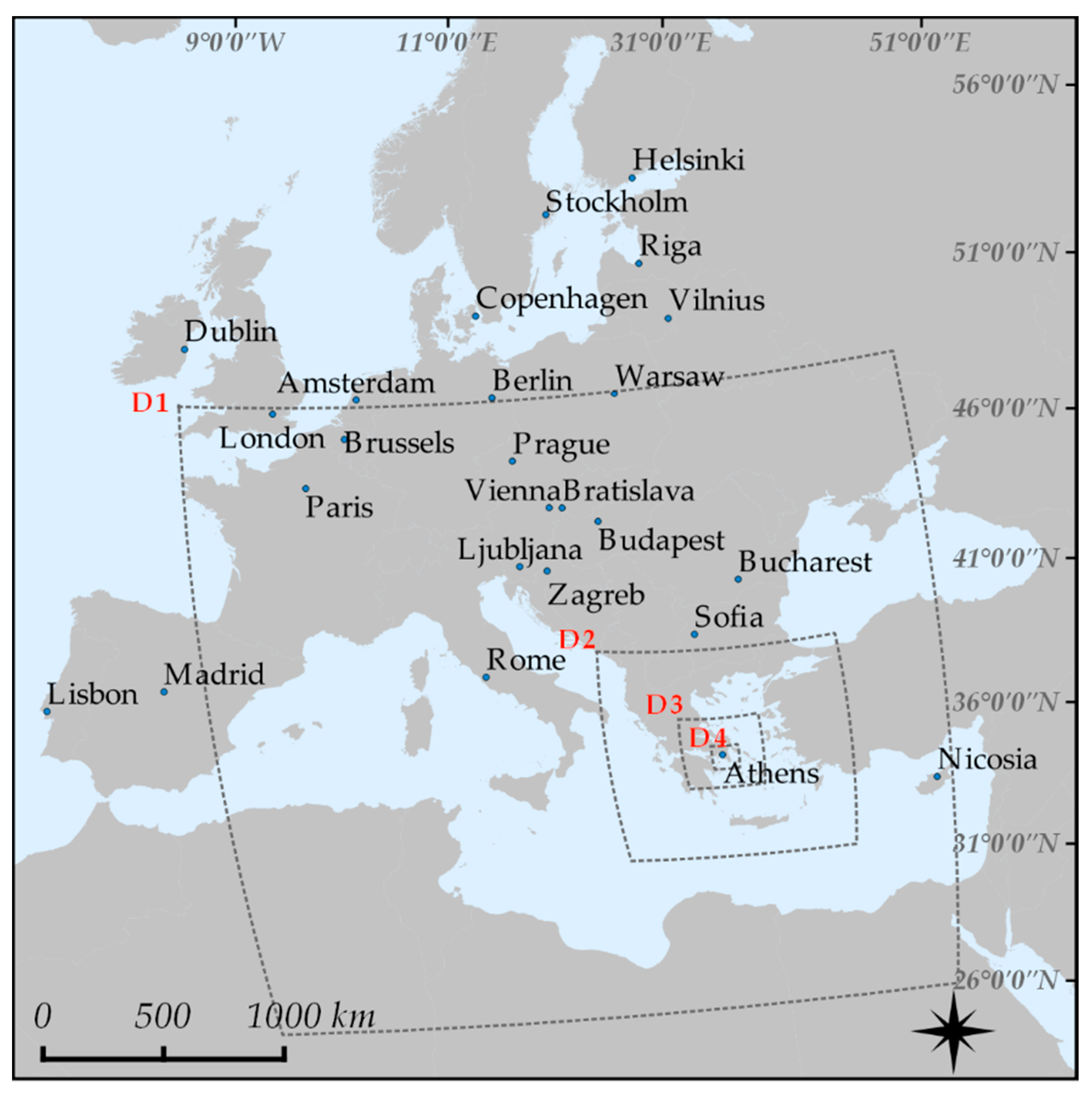
3.1. Overall Results for European Cities

The number of the available clear-sky MODIS–LST imagery for the period June to August 2017 varied significantly across cities, from 38 images for Amsterdam to 245 for Lisbon (average value: 119 images per city). Intra-urban spatial variability was found approximately twice as high during daytime compared to nighttime, with an average LST standard deviation of 2.1 K and 1.1 K, respectively. After normalization, the LST products MOD11A1 and MYD11A1 showed high similarity for each study area, for both their daytime and nighttime average LSTs (rho = 0.886 and non-statistically significant differences after a paired sample t-test). Thereby, the thermal spatial patterns and the statistical analysis for a given city were to a great extent overlapping between the two MODIS satellites; thus, the results presented in this section were derived only from Aqua (MYD11A1 product), which corresponds to overpassing times at fully developed daytime and nocturnal urban boundary layers.

Spearman’s rho linear correlation coefficients between the urban surface parameters and LST by day are presented in

Table 4. Spearman’s rho linear correlation between the urban surface parameters and LST (MODIS–Aqua) during daytime for all cities.

City	Correlation with LST			City	Correlation with LST
	λimp	λb	H		λimp	λb	H
Amsterdam	0.59	0.48	0.53	Madrid	−0.21	−0.52	−0.37
Athens	0.55	0.34	0.06	Nicosia	−0.58	−0.66	−0.47
Berlin	0.78	0.63	0.53	Paris	0.74	0.51	0.41
Bratislava	0.44	0.26	−0.02	Prague	0.70	0.61	0.53
Brussels	0.77	0.47	0.44	Riga	0.71	0.69	0.14
Bucharest	0.72	0.58	0.40	Rome	0.07	−0.08	−0.01
Budapest	0.64	0.46	0.42	Sofia	0.67	0.46	0.40
Copenhagen	0.66	0.54	0.26	Stockholm	0.57	0.55	0.26
Dublin	0.70	0.65	0.12	Vienna	0.64	0.59	0.40
Helsinki	0.57	0.43	0.31	Vilnius	0.73	0.57	0.67
Lisbon	0.24	0.05	0.24	Warsaw	0.71	0.48	0.59
Ljubljana	0.76	0.67	0.58	Zagreb	0.79	0.70	0.64
London	0.65	0.55	0.29

. For the majority of the cities the λ_imp–LST relationship had a statistically significant positive correlation (p < 0.05), with an average value for all cases of rho = 0.54. For cities characterized by warmer and dryer summer conditions (southern European cities; Bsh and Csa climate types in Table 1), the correlation was noticeably weaker and, in two cases, negative (Nicosia and Madrid). Bivariate correlations between λ_imp and the other two surface features were also high; mainly for the case of λ_b (average rho = 0.83) and to a lesser extent for H (rho = 0.54)—all the pairwise correlations among the three morphological parameters can be found in the Appendix A (

Table A1. Pairwise Spearman’s rho linear correlations among λ_imp, λ_b, and H.

		λimp	λb	H			λimp	λb	H
Amsterdam	λimp	1.00	0.83	0.53	London	λimp	1.00	0.83	0.48
	λb	0.83	1.00	0.40		λb	0.83	1.00	0.38
	H	0.53	0.40	1.00		H	0.48	0.38	1.00
Athens	λimp	1.00	0.82	0.46	Madrid	λimp	1.00	0.77	0.51
	λb	0.82	1.00	0.66		λb	0.77	1.00	0.47
	H	0.46	0.66	1.00		H	0.51	0.47	1.00
Berlin	λimp	1.00	0.83	0.59	Nicosia	λimp	1.00	0.94	0.49
	λb	0.83	1.00	0.55		λb	0.94	1.00	0.43
	H	0.59	0.55	1.00		H	0.49	0.43	1.00
Bratislava	λimp	1.00	0.91	0.46	Paris	λimp	1.00	0.83	0.53
	λb	0.91	1.00	0.45		λb	0.83	1.00	0.34
	H	0.46	0.45	1.00		H	0.53	0.34	1.00
Brussels	λimp	1.00	0.69	0.63	Prague	λimp	1.00	0.93	0.63
	λb	0.69	1.00	0.50		λb	0.93	1.00	0.66
	H	0.63	0.50	1.00		H	0.63	0.66	1.00
Bucharest	λimp	1.00	0.83	0.33	Riga	λimp	1.00	0.86	0.24
	λb	0.83	1.00	0.34		λb	0.86	1.00	0.13
	H	0.33	0.34	1.00		H	0.24	0.13	1.00
Budapest	λimp	1.00	0.74	0.56	Rome	λimp	1.00	0.88	0.58
	λb	0.74	1.00	0.27		λb	0.88	1.00	0.51
	H	0.56	0.27	1.00		H	0.58	0.51	1.00
Copenhagen	λimp	1.00	0.85	0.48	Sofia	λimp	1.00	0.89	0.57
	λb	0.85	1.00	0.34		λb	0.89	1.00	0.61
	H	0.48	0.34	1.00		H	0.57	0.61	1.00
Dublin	λimp	1.00	0.89	0.22	Stockholm	λimp	1.00	0.56	0.61
	λb	0.89	1.00	0.05		λb	0.56	1.00	0.15
	H	0.22	0.05	1.00		H	0.61	0.15	1.00
Helsinki	λimp	1.00	0.79	0.58	Vienna	λimp	1.00	0.85	0.77
	λb	0.79	1.00	0.27		λb	0.85	1.00	0.58
	H	0.58	0.27	1.00		H	0.77	0.58	1.00
Lisbon	λimp	1.00	0.89	0.59	Vilnius	λimp	1.00	0.86	0.61
	λb	0.89	1.00	0.52		λb	0.86	1.00	0.47
	H	0.59	0.52	1.00		H	0.61	0.47	1.00
Ljubljana	λimp	1.00	0.93	0.70	Warsaw	λimp	1.00	0.76	0.61
	λb	0.93	1.00	0.64		λb	0.76	1.00	0.45
	H	0.70	0.64	1.00		H	0.61	0.45	1.00
					Zagreb	λimp	1.00	0.91	0.66
						λb	0.91	1.00	0.52
						H	0.66	0.52	1.00

). Thus, not surprisingly, λ_b showed a somewhat similar connection to LST in the daytime (average rho = 0.40) as that of λ_imp. The pairwise relation of H with LST yielded higher variability across cities and generally lower rho values (average rho = 0.29). Depending on the city, the H–LST correlation varied from strongly negative (e.g., Madrid) or with no obvious association (e.g., Athens, London) to moderately/strongly positive—for most cases. Nighttime correlations (

Table 5. As in Table 4, for observations during nighttime.

City	Correlation with LST			City	Correlation with LST
	λimp	λb	H		λimp	λb	H
Amsterdam	0.42	0.36	0.46	Madrid	0.58	0.55	0.53
Athens	0.78	0.77	0.58	Nicosia	0.54	0.60	0.45
Berlin	0.59	0.55	0.70	Paris	0.71	0.58	0.52
Bratislava	0.49	0.49	0.45	Prague	0.64	0.65	0.67
Brussels	0.53	0.59	0.63	Riga	0.51	0.42	0.30
Bucharest	0.50	0.48	0.78	Rome	0.69	0.67	0.73
Budapest	0.62	0.43	0.49	Sofia	0.59	0.63	0.45
Copenhagen	0.49	0.55	0.50	Stockholm	0.28	0.34	0.28
Dublin	0.59	0.72	0.01	Vienna	0.50	0.43	0.53
Helsinki	0.50	0.46	0.53	Vilnius	0.45	0.53	0.54
Lisbon	0.47	0.44	0.48	Warsaw	0.53	0.43	0.68
Ljubljana	0.57	0.53	0.61	Zagreb	0.46	0.37	0.33
London	0.63	0.55	0.41

) were generally more consistent across study areas. All measures of cover and structure were detected to be strongly, positively correlated with LST at night; average rho was equal to 0.55, 0.52, and 0.51 for λ_imp, λ_b, and H, respectively. Hence, in contrast to daytime hours, H at night was found positively correlated to LST in all but one case (Dublin) and with rho values of similar magnitude to those for λ_imp. It should be noted that all results in Table 4 and Table 5 correspond to statistically significant correlations (p < 0.05), except for the λ_imp–LST and H–LST correlations for daytime Rome.

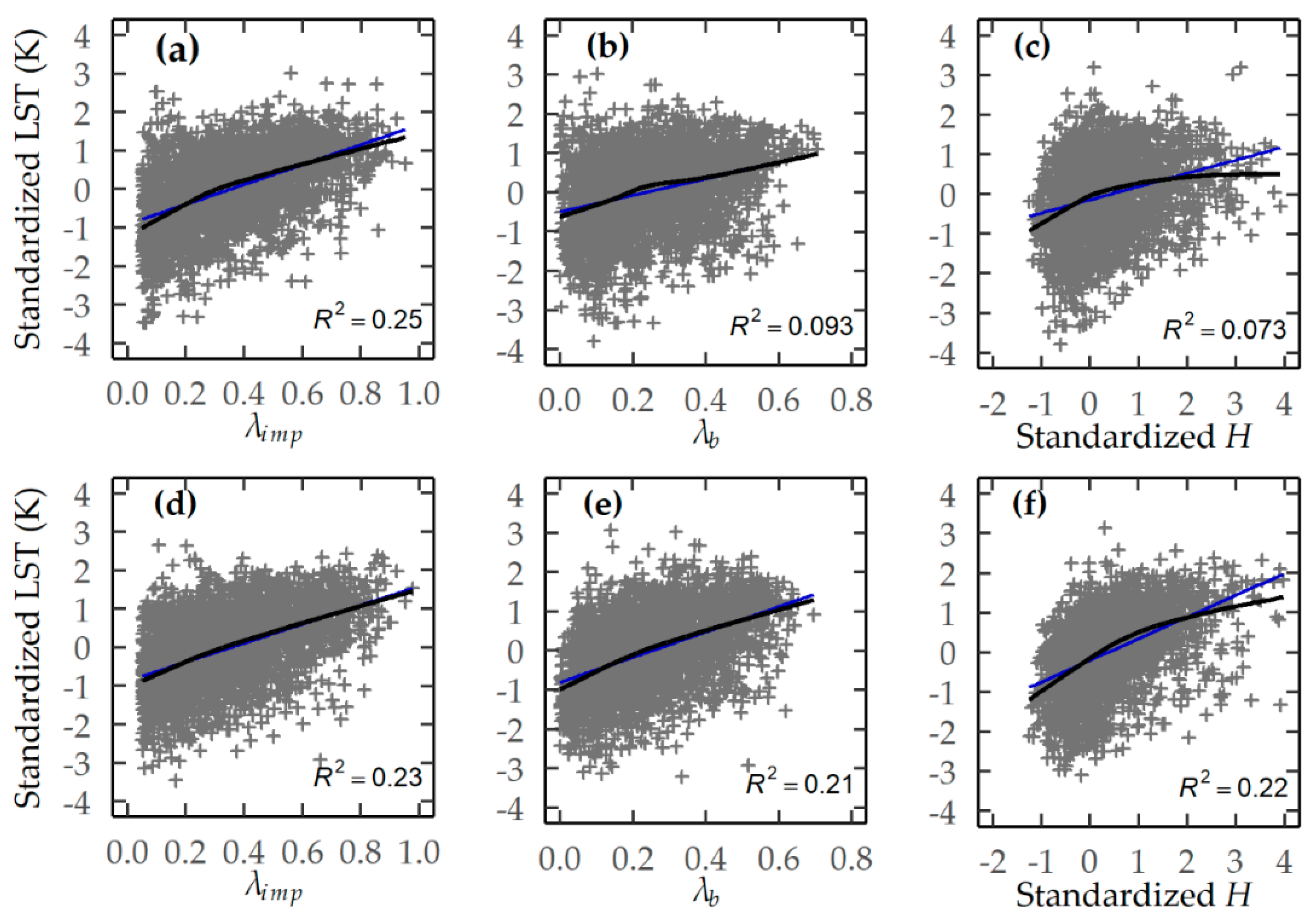
The relationship between the examined urban features and MODIS–LST was examined in more detail using scatter plots and deriving the non-parametric best fitting functions from lowess regression. For λ_imp an almost linear relation with LST was determined, observed both in daytime and nighttime observations. This relationship was obtained both when examining each city independently (not shown) and when aggregating all study areas, as presented in Figure 5a,d. To avoid oversampling the larger cities in Figure 5, 100 randomly distributed pixels for each case were prior selected. A similar, approximately linear relationship was obtained for λ_b–LST (Figure 5b,e). Greater complexity can be observed for the relationship of H and LST. Specifically, during daytime (Figure 5c), for the values above a critical building height (approximately one standard deviation above the mean H), the lowess regression results in a less steep increasing curve, while no obvious relation can be observed. A significant number of observations can also be detected in the upper left region of Figure 5c—corresponding to low H and high LST. At night (Figure 5f), LST was found to increase more consistently with H.

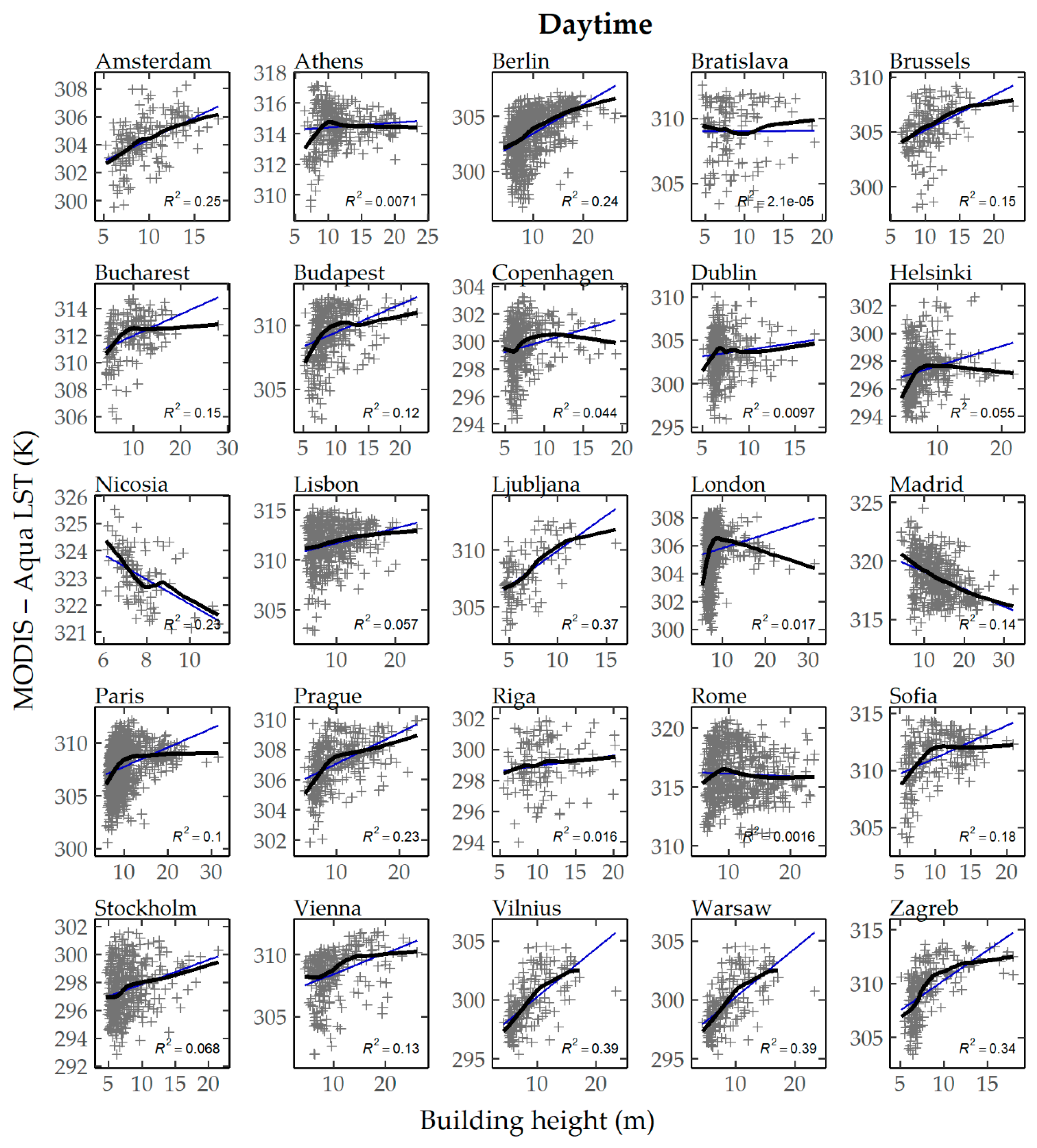
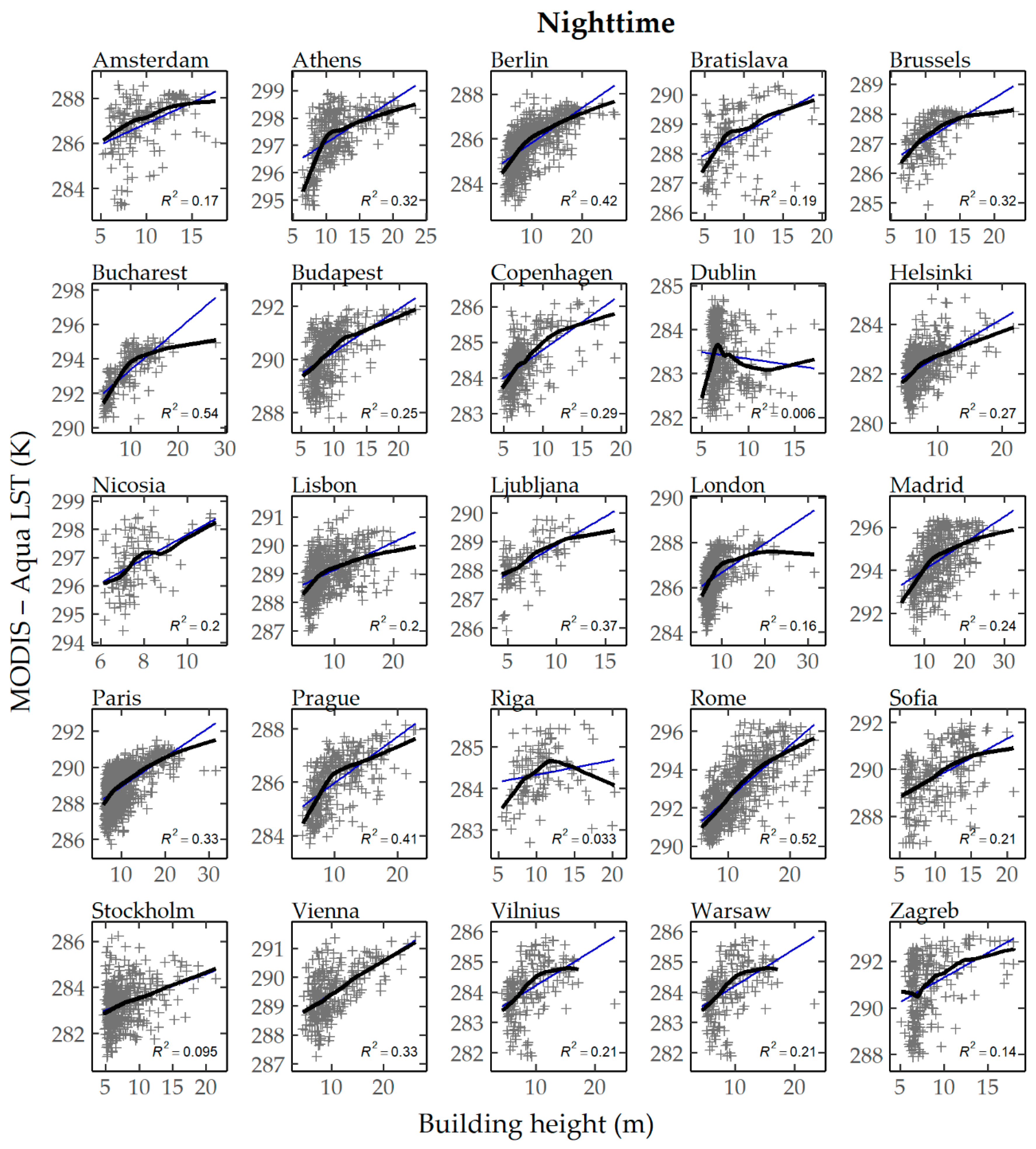
To achieve a more detailed investigation of the H–LST relationship, the individual scatter plots and the associated lowess regression fit per city are given in Figure 6 and Figure 7. In Figure 6 (daytime surface temperatures) several distinguishing interlinks can be detected across study areas. For a significant number of occasions—most noticeably for Athens, Copenhagen, Paris, and London—daytime LST increased approximately linearly up to maximum value at intermediate heights, above which the positive association levels off or is reversed. In a few cities (e.g., Amsterdam and Brussels) as H increased, LST values were consistently larger. Finally, mainly for southern/Mediterranean cities, a particularly weak (Lisbon and Rome) or negative (Madrid and Nicosia) relation between H and LST was observed. Conversely, during nighttime (Figure 7) H and LST presented a more consistent association across cities; LST was positively affected by increasing building height for the vast majority of the examined cases.

As noted previously, strong intercorrelations were found for λ_imp, λ_b, and H; thereby the independent effect of each variable on LST may to an extent be concealed in the pairwise correlations. The relative influence of each surface parameter after adjusting for the others was assessed within multiple regression models. The overall results of the regression analysis are given in

Table 6. Standardized regression coefficients and coefficient of determination R² for the multiple regression models between the urban surface parameters and LST.

City	Daytime				Nighttime
	λimp	λb	H	R2	λimp	λb	H	R2
Amsterdam	0.44 ***	0.03	0.24 ***	0.40	0.24	0.03	0.26 **	0.22
Athens	0.75 ***	−0.16	−0.15 **	0.36	0.48 ***	0.24 ***	0.17 ***	0.64
Berlin	0.81 ***	−0.11 *	0.04	0.56	0.17 **	0.18 ***	0.45 ***	0.49
Bratislava	0.56 ***	–	−0.25 **	0.25	0.36 ***	–	0.27 **	0.30
Brussels	0.89 ***	−0.10	−0.11	0.58	−0.02	0.44 ***	0.37 ***	0.46
Bucharest	0.72 ***	−0.06	0.16 **	0.54	0.22 *	0.16	0.61 ***	0.66
Budapest	0.65 ***	−0.01	−0.06	0.36	0.45 ***	0.06	0.20 ***	0.40
Copenhagen	0.84 ***	−0.13	−0.16 **	0.44	−0.23 **	0.62 ***	0.49 ***	0.48
Dublin	0.65 ***	0.03	−0.08	0.44	−0.21 *	0.89 ***	−0.06	0.51
Helsinki	0.90 ***	−0.21 **	−0.27 ***	0.34	−0.13	0.38 ***	0.48 ***	0.35
Lisbon	0.80 ***	−0.71 ***	0.15 **	0.19	0.23 **	0.14	0.26 ***	0.29
Ljubljana	0.69 ***	–	0.11	0.61	0.33 **	–	0.37 ***	0.42
London	0.71 ***	0.05	−0.24 ***	0.45	0.37 ***	0.23 ***	0.15 ***	0.42
Madrid	0.50 ***	−0.79 ***	−0.26 ***	0.40	0.34 ***	0.17 **	0.25 ***	0.43
Nicosia	−0.48 ***	–	−0.30 ***	0.43	0.43 ***	–	0.28**	0.36
Paris	1.13 ***	−0.40 ***	−0.15 ***	0.59	0.53 ***	0.02	0.27 ***	0.54
Prague	0.62 ***	–	0.11 *	0.48	0.42 ***	–	0.39 ***	0.52
Riga	0.48 ***	0.22	−0.01	0.47	0.39 *	0.12	0.08	0.27
Rome	0.73 ***	−0.70 ***	−0.10 *	0.12	0.27 ***	0.18 ***	0.47 ***	0.65
Sofia	1.06 ***	−0.63 ***	0.21 ***	0.49	0.16	0.44 ***	0.09	0.43
Stockholm	0.41 ***	0.32 ***	−0.10 *	0.36	−0.12	0.34 ***	0.28 ***	0.17
Vienna	0.69 ***	0.15	−0.25 **	0.43	0.02	0.17	0.47 ***	0.35
Vilnius	0.63 ***	−0.06	0.32 ***	0.64	−0.33 **	0.67 ***	0.37 ***	0.38
Warsaw	0.85 ***	–	−0.30 ***	0.42	0.20 *	–	0.41 ***	0.44
Zagreb	0.67 ***	–	0.17 **	0.62	0.42 ***	–	0.12	0.25

*** p < 0.001; ** p < 0.01; * p < 0.05.

, where regression coefficients are standardized (beta coefficients).

The main findings for the surface influences during daytime can be summarized as follows: The impervious fraction (λ_imp) was shown to be the stronger controlling factor of LST; for almost all cities it had statistically significant positive beta coefficients, larger in magnitude than λ_b and H. Besides, it can be observed that after adjusting for the other two surface parameters, λ_imp exerted a positive influence on LST also for all southern European cities. Regarding λ_b and H, the sign and statistical significance of beta coefficients had larger variability among different study areas. However, all statistically significant coefficients for λ_b were negative (apart from Stockholm), with a value ranging between −0.88 and −0.10. For H, cities with a consistent positive relationship in Figure 6, resulted in positive regression coefficients. On the other hand, when daytime LST was decreasing with increasing H or had a peak at intermediate heights, the regression coefficients were statistically significant negative, however, with a weaker effect on LST than that exerted by λ_imp.

For nighttime observations, the strength and direction of the influence on LST was found to be much more evenly distributed among surface parameters. The impervious fraction was no longer the prevailing determining factor of LST; in some cases, it had a negative association with LST, however, for the majority of the statistically significant beta coefficients, the effect was positive. For λ_b and H, the nighttime regression results were noticeably different from those by day. Firstly, for the majority of the cases, beta coefficients increased in value, which was often accompanied by a change of their sign. Furthermore, the statistically significant coefficients for λ_b and H were positive and of similar magnitude to those for λ_imp.

The coefficient of determination (R²) of the multiple regression models had an average value of 0.45 and 0.42 in daytime and nighttime, respectively. Despite the intercorrelation between surface paraments, the multicollinearity metric VIF had moderate values, below the theoretical, critical threshold of 5 (average VIF for all regression models: 3.40). As can be seen in Table 6 for six cities, that the original regression models resulted in a VIF value over 5, only λ_imp and H were finally included in the analysis to avoid the emerging multicollinearity effects.

Besides the central role of urban morphology discussed above, sea breeze has also been found to be an important determinant of the urban heat island intensity, usually exerting a strong moderating influence [101,102,103]. To include the effects of the sea breeze in the current statistical analysis, further regression models were developed incorporating the proximity to the sea—the distance between the center of a given image pixel and the coastline (d)—as an additional independent variable. Only the urban areas within ten kilometers of the coast were considered, in order to ensure a strong influence of the local sea breeze circulation, irrespective of other local characteristics of each study area. As can be seen from

Table 7. Standardized regression coefficients for the multiple regression models between the urban surface parameters, proximity to the sea, and LST for seven coastal urban areas.

City	Daytime				Nighttime
	λimp	λb	H	d	λimp	λb	H	d
Athens	0.60 ***	−0.10	−0.52 ***	0.21 **	0.32 ***	0.46 ***	0.01 ***	−0.17 ***
Copenhagen	0.93 ***	−0.28 **	−0.16 **	0.20	−0.12 **	0.46 ***	0.53 ***	0.06
Dublin	0.42 ***	0.30 **	−0.05	0.46 ***	−0.24 **	0.95 ***	−0.09	0.17 ***
Helsinki	0.68 ***	0.02 **	−0.26 ***	0.15 **	−0.06	0.23 ***	0.29 ***	−0.44 ***
Lisbon	0.80 ***	−0.64 ***	0.08	0.23 ***	0.23**	0.06	0.31 ***	−0.29 ***
Riga	0.21	0.29	0.03	0.36 **	0.36	−0.01	0.12	−0.52 **
Rome	0.53 **	−0.35 *	−0.28 **	0.65	0.22	0.36	0.41 ***	0.09

*** p < 0.001; ** p < 0.01; * p < 0.05.

, during daytime for all the examined urban areas, a larger distance from the coast resulted in higher surface temperatures. For five of the seven cases, the cooling effect of the sea breeze was also found to be statistically significant. At night, the developing land breeze provided more diverging results—which may be attributed to local influences not taken into account in the current analysis. Nevertheless, as expected, for the majority of the nighttime cases, the proximity to the sea results in a positive influence on LST. In addition, the statistically significant results of all 4-variable regression models were in agreement with the findings presented previously (Table 6) regarding the control of urban form—i.e., that closely packed and/or high-rise buildings tend to result in lower temperatures during daytime and to higher LST values at night.

Statistically significant and relatively high was the spatial autocorrelation of the multiple regression models. The average Moran’s I measure of spatial autocorrelation was found equal to 0.61 in the daytime and 0.66 at nighttime. Hence, spatial regression models were used to incorporate in the analysis of the neighboring influences on the LST values. Specifically, spatial lag models (SLM) were developed, assuming that the spatial influence was constrained to the eight direct neighbors of a given pixel. Different choices regarding the adjacency weights did not lead to improved accuracy, thus were not included in the findings. A summary of the spatial regression results is given in

Table 8. Standardized regression coefficients (total effect) for the spatial regression models SLM between the urban surface parameters and LST.

City	Daytime			Nighttime
	λimp	λb	H	λimp	λb	H
Amsterdam	0.75 *	0.29	0.22	1.27	0.02	−0.18
Athens	2.76 ***	−0.88	−1.48 **	0.98 ***	1.03 ***	−0.15
Berlin	2.13 ***	−0.10	−0.54 ***	0.30	1.02 ***	0.56 **
Bratislava	1.30 **	–	−0.30	0.75 **	–	0.65 *
Brussels	3.20 *	0.57	−0.61	0.58	2.60 ***	1.22 **
Bucharest	1.36 ***	−0.25	0.10	0.44	0.29	1.00 ***
Budapest	1.82 ***	0.26	−0.71 **	1.11 *	1.23 ***	−0.21
Copenhagen	2.51 ***	−0.01	−0.74 ***	−0.34	1.57 ***	0.58 *
Dublin	2.72 ***	−0.68	−0.49 *	1.40 **	0.62	−0.50 *
Helsinki	3.18 ***	−0.71*	−0.98 ***	−0.21	0.83 **	0.73 **
Lisbon	2.10 ***	−1.28 **	−0.12	0.98	−0.14	0.85 *
Ljubljana	1.64 ***	–	−0.05	1.64 ***	–	0.44
London	3.41 ***	−0.32	−1.52 ***	1.78 ***	0.47	−0.39
Madrid	1.00 ***	−1.59 ***	−0.54 **	1.13 ***	0.46 *	0.47 **
Nicosia	−2.01 ***	–	−0.47	2.80 ***	–	−0.15
Paris	2.67 ***	−0.47 **	−0.76 ***	1.43 ***	0.53 *	0.07
Prague	1.97 ***	–	−0.35 *	1.51 ***	–	1.08 ***
Riga	0.91 *	0.57	−0.02	0.25	1.05	0.52
Rome	2.97 ***	−2.69 ***	−0.83**	0.84 ***	0.58**	0.47 ***
Sofia	2.69 ***	−1.31 ***	0.21	0.41	1.81 **	−0.12
Stockholm	1.47 ***	0.60 ***	−0.56 ***	−0.61	1.03 ***	0.49
Vienna	4.45 ***	–	−1.88 ***	1.83 **	–	0.57
Vilnius	2.04 ***	−0.57 **	0.14	0.06	1.64 **	−0.02
Warsaw	1.78 ***	–	−0.06	1.02 **	–	1.24 **
Zagreb	1.76 ***	–	−0.12	0.78 *	–	0.79 *

*** p < 0.001; ** p < 0.01; * p < 0.05.

; regression coefficients are standardized, and they correspond to the total influence—the sum of direct and indirect effects—of the independent variables according to [104].

The results of SLM models were generally in agreement with the OLS regression regarding the direction of urban structure controls on LST. By day, on almost all occasions, the statistically significant spatial regression coefficients were positive for λ_imp and negative—also smaller in magnitude—for λ_b and H. In contrast, during nighttime, almost all statistically significant coefficients were positive for all three surface parameters. In some cases, non-statistically significant sign changes were observed in comparison to the multiple regression results. An inter-comparison of the accuracy of the two regression types can be derived using the Akaike information criterion (AIC), where a lower value corresponds to better performance of the model. The reduction of AIC when using SLM—by an average of 67% in the daytime and 81.6% at night compared to the OLS regression—highlights the improvement in modeling LST when spatial autocorrelation was taken into account.

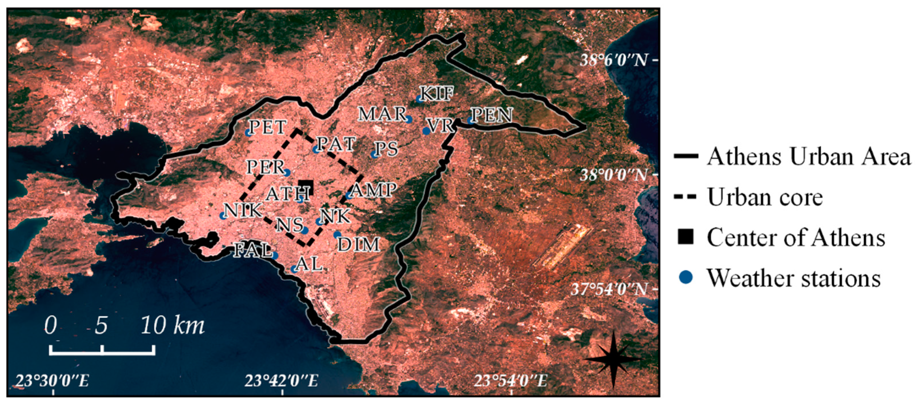
3.2. Urban Area of Athens

In the previous section, a broad statistical assessment of the relation between surface parameters and LST was conducted for 25 European cities. A more focused analysis was carried out next for the city of Athens in order to highlight the aspects of urban form and the physical processes that drive the derived associations. A point of concern in the previous discussion was the high intercorrelations among λ_imp, λ_b, and H. It is common that in urban areas, impervious fraction, building density, and building height increase largely concurrently—typically from the city outskirts to the city center [105]. Although multiple regression allows the isolation of the independent effect of a given variable, statistical analysis is accompanied by uncertainties and its underlying assumptions are not fully satisfied in practice. The particular characteristics of the urban environment of Athens enable us to define well-distinguished zones of differing three-dimensional structures, controlling in this way for vegetation variations.

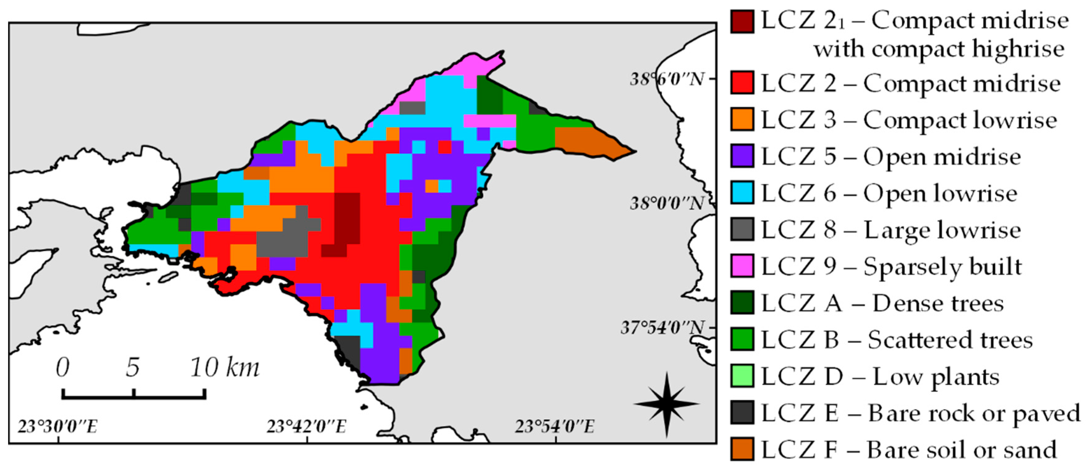
As follows from Figure 3, a clear division can be observed for Athens, between the well-vegetated, less densely built northeastern part of the city (to a lesser extent also for the southeastern districts) and the central areas. Focusing on the urban core—as defined in Figure 2—the following characteristics can be outlined: The inner-city area (LCZ 2₁ and LCZ 2, Figure 4) corresponds to neighborhoods of dense and high-rise structure; vegetation is generally scarce except for few fragmented urban parks (see Figure 2). In close proximity, there is an extended area of light industrial use, mainly with open set low-rise buildings (LCZ 8). Moreover, the western districts of the urban core correspond to compact housing with medium/low building height (LCZ 2 and mostly LCZ 3).

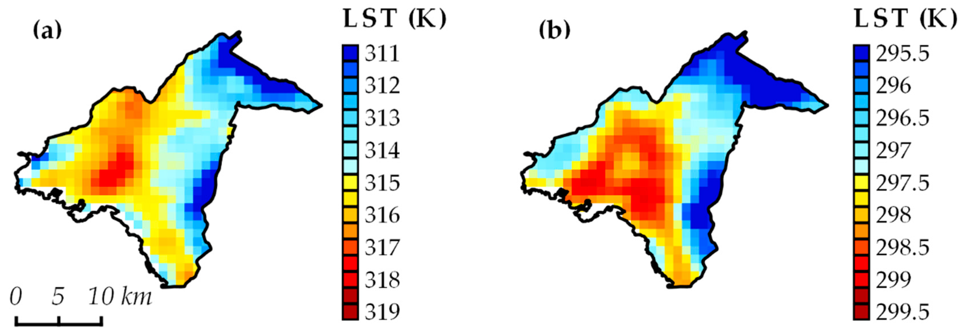
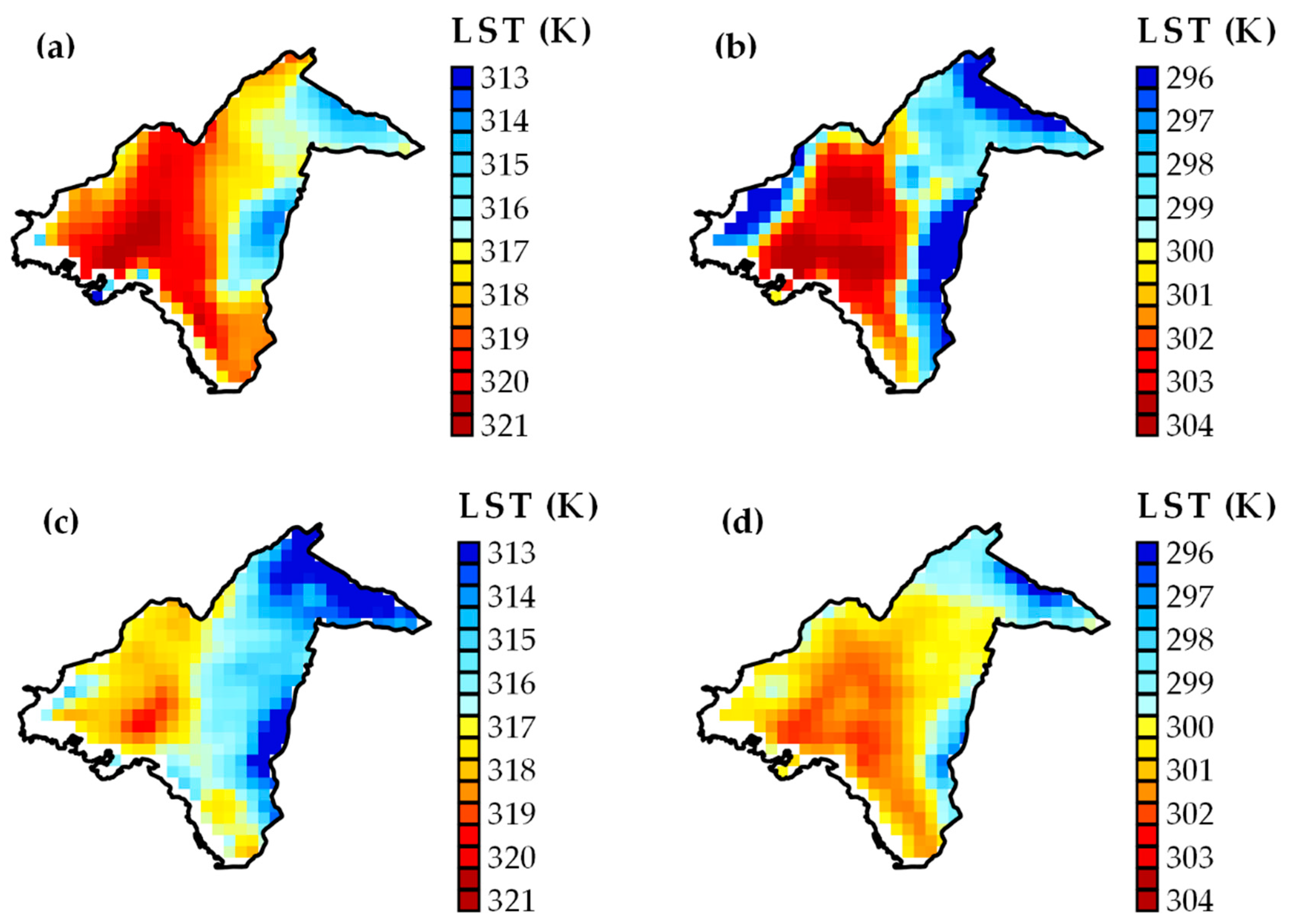
For all the above-mentioned zones, vegetation density is low and similar across the LCZs; the average λ_imp inside the urban core was found equal to 0.66, 0.66, 0.70, and 0.69 for LCZ 2₁, LCZ 2, LCZ 3, and LCZ 8, respectively. For this calculation, as well as in the following discussions, three pixels inside the urban core that include extended urban parks were not taken into account. Figure 8 shows the average surface temperature of Athens during the summer months of 2017 using the product MODIS LST product (clear sky observations of Aqua). It can be observed that the northeastern regions of the urban area were associated, both during daytime and nighttime, with lower surface temperatures. That is in accordance to the results of Figure 5 and Table 6 and Table 7 for Athens, regarding the negative relation of λ_imp with LST. Overall, the classes LCZ 5, 6, and 9 had an average lower LST by ≈ 1.9 Κ in comparison to the other urban LCZs. Of more interest is the spatial variability inside the urban core of the city. There, during daytime pixels included in the LCZ 8 class (high values of λ_imp and relatively low values of λ_b and H) were clearly distinguished as the warmer spots in Athens (LST ≈ 317 K). The districts where closely-packed, high-rise buildings prevail (LCZ 2₁) were characterized by notably lower temperatures (LST ≈ 315.3 K). Thus, the negative relation of H with daytime LSTs that was previously derived for Athens using multiple regression analysis (Table 6) can also be detected here. The western periphery tends to be characterized by intermediate values of λ_b and H that was subsequently mirrored in the observed LSTs. The thermal patterns of the urban core were reversed when examining the nighttime spaceborne observations: The densely built-up neighborhoods exhibited in this case higher LST than the LCZ 8 zone. In

Table 9. Mean (± one standard deviation), minimum and maximum land surface temperature (degrees Kelvin) for remotely-sensed MODIS–AQUA in Athens per LCZ (June–August 2017).

	Daytime			Nighttime
	Mean	Min	Max	Mean	Min	Max
LCZ 21	315.3 ± 0.3	314.6	315.8	298.6 ± 0.2	298.4	299.0
LCZ 2	315.3 ± 0.8	313.8	317.1	298.2 ± 0.6	296.5	299.0
LCZ 3	316.1 ± 0.6	314.0	316.8	298.2 ± 0.4	297.3	298.8
LCZ 5	314.6 ± 0.8	312.7	316.2	297.4 ± 0.6	296.2	298.5
LCZ 6	314.3 ± 1.6	310.7	316.8	296.7 ± 0.8	294.9	298.1
LCZ 8	317.1 ± 0.9	314.3	317.9	297.9 ± 0.8	295.7	298.6
LCZ 9	313.3 ± 1.5	310.6	316.2	295.5 ± 0.5	294.8	296.8

, the overall surface temperature statistics are shown per LCZ (natural type LCZs were not included).

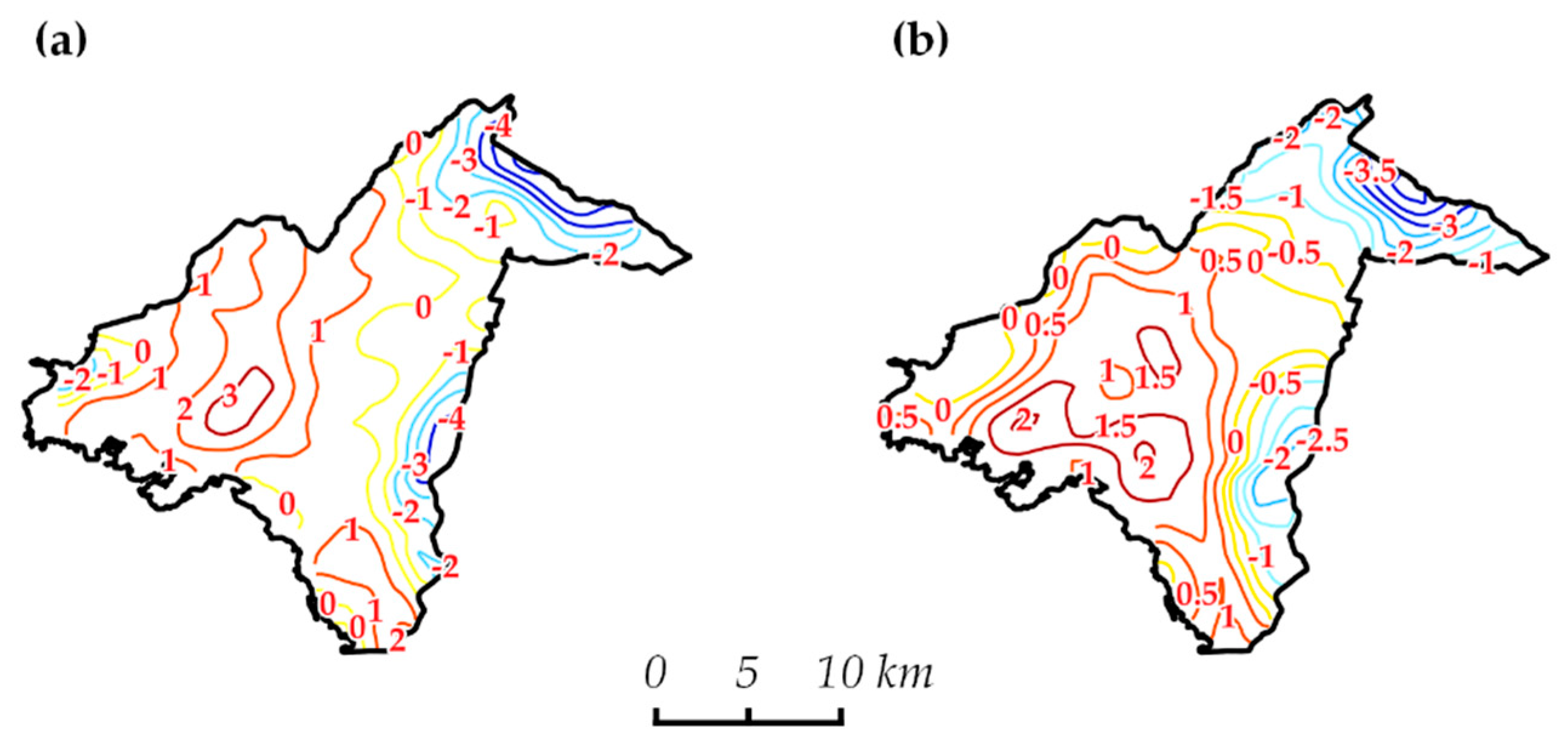
The local differentiations across the city can be more clearly outlined deriving the normalized—the temperature anomaly relative to the average value of LST for the study area—isotherms. As can be observed in Figure 9, the center of the LCZ 8 class was by day, on average, 3 °C warmer than the average temperature of the study area and up to 2 °C than the neighboring densely built central area. At night—where in general LST variability was weaker—a local minimum can be detected in LCZ 8, with a lower LST up to 1 °C compared to the adjacent areas. Furthermore, in the broader region, three distinct centers of excess heat were developed.

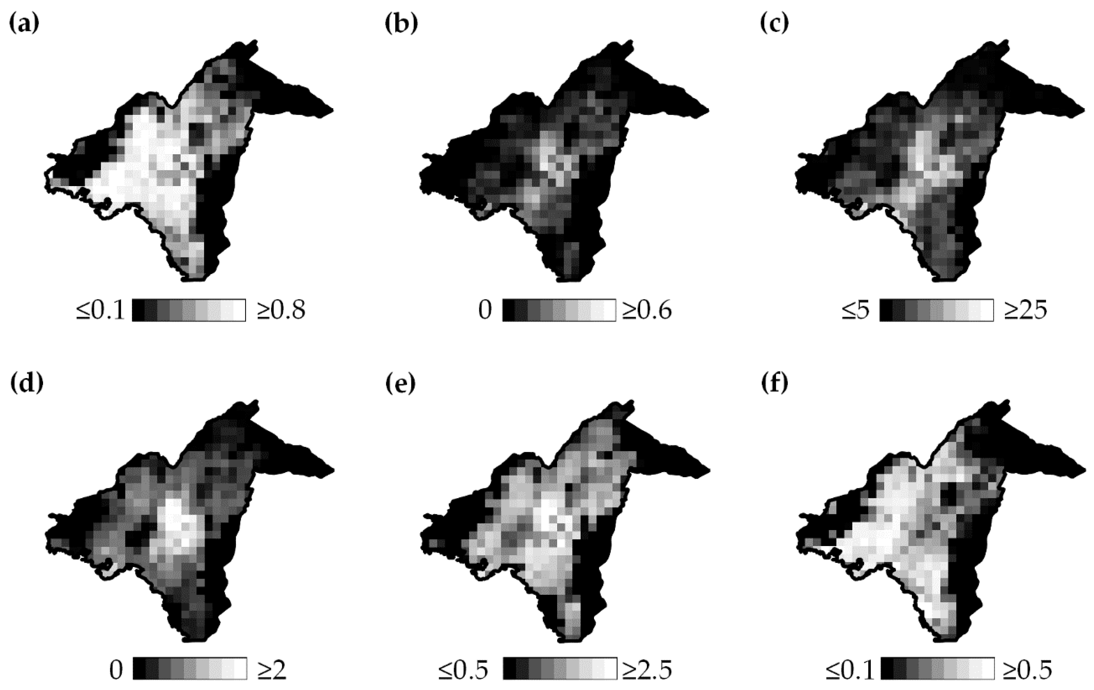
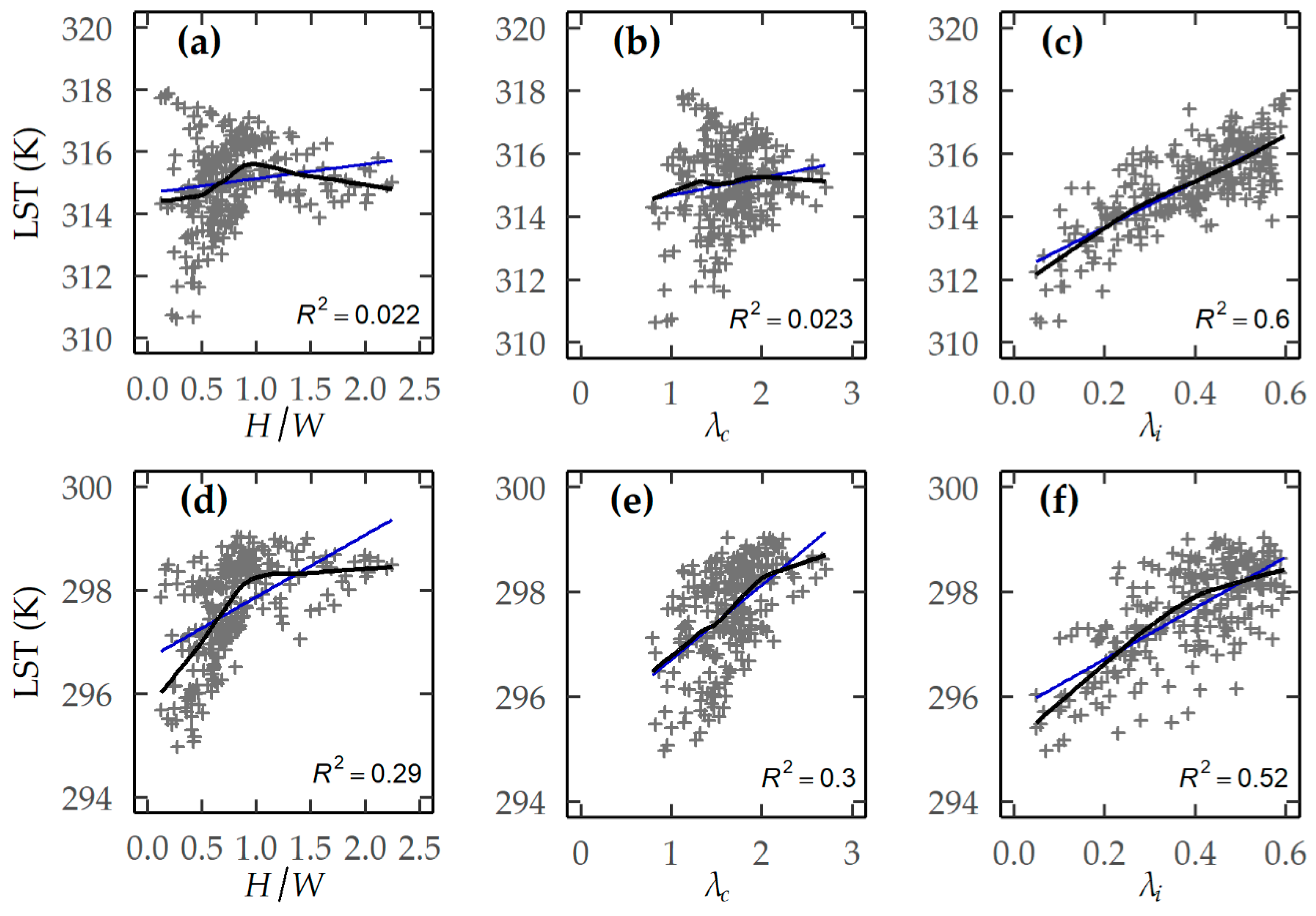
The thermal signature of the local climate zones is driven by the vegetation density and the characteristics of urban structure, with the latter being the determining influence for the urban core of Athens. In Section 3.1, the average building height H was used as a means of accounting the total three-dimensional effects (i.e., used as a proxy variable). Figure 10 shows the relation of LST with two additional surface parameters of the urban structure (H/W and λ_c) and a parameter that describes the fraction of impervious ground (i.e., impervious surface without buildings) (λ_i). During the daytime, H/W had a similar association with LST, as shown previously for H in Figure 6. Specifically, LST is increasing with H/W for the range 0 to ≈1, while for larger height-to-width ratios, there is a noticeable decline in LSTs. No obvious relation is found for λ_c (Figure 10b), whereas λ_i (Figure 10c) shows a remarkable linearity and strong correlation with LST (rho = 0.70, p <0.01). For nighttime observations, all three parameters exerted a positive influence on LSTs (Figure 10d–f).

The surface temperatures of the urban districts of Athens in close proximity to the sea were expected to be influenced by the presence of the local sea breeze circulation. To quantify the magnitude of this effect, the sea breeze days for June–August 2017 were firstly identified, considering the cases when the wind direction was between 150° and 280° during daytime hours and between 300° and 130° at night [106]. For the remaining dates, the city was under the influence of the synoptic flow (northern wind). As seen from

Table 10. Mean land surface temperature (degrees Kelvin) for remotely-sensed MODIS–AQUA in Athens per LCZ, per circulation type, and per distance (d) to the coastline during daytime (June–August 2017).

	Sea Breeze		Synoptic Flow
	d < 3 km	d > 3 km	d < 3 km	d > 3 km
LCZ 2	314.5	315.0	314.7	314.4
LCZ 3	314.8	315.7	315.2	315.6
LCZ 5	314.4	314.5	314.6	313.7
LCZ 6	315.0	314.2	315.0	313.5

, depending on the circulation type, the neighborhoods that were close to the seashore—distance lower than 3 km—were generally relatively cooler during daytime and warmer at night, in agreement to Table 7.

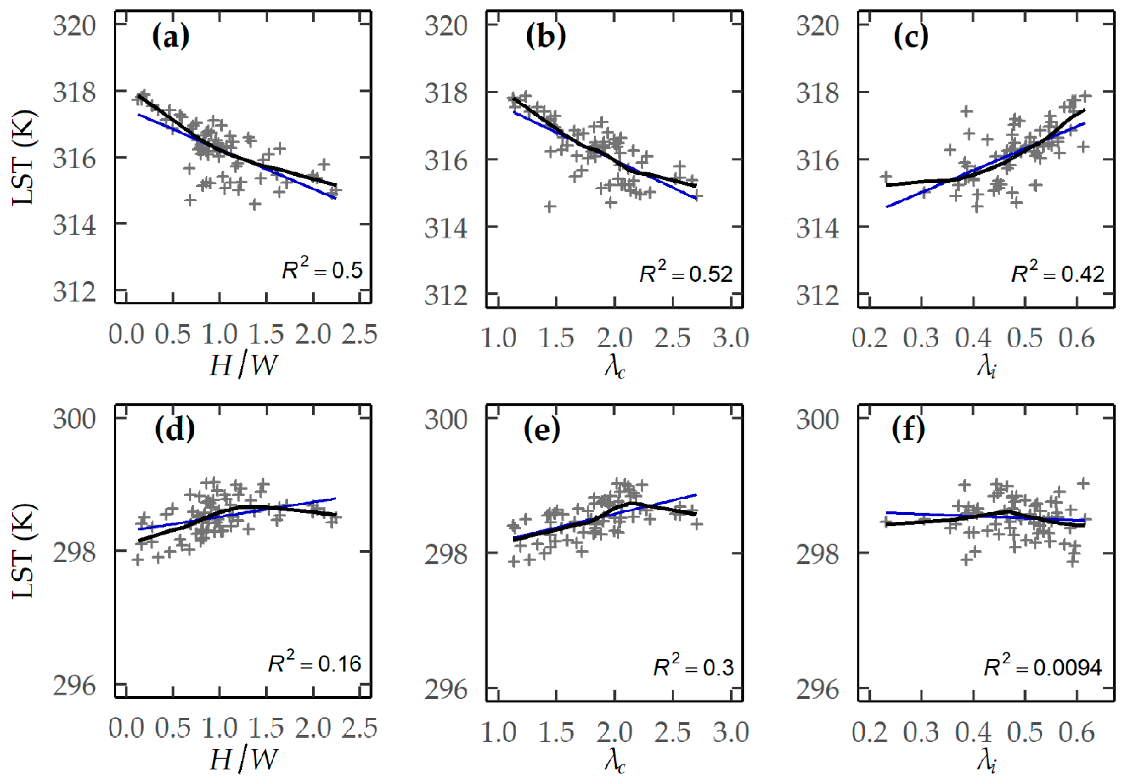
To isolate the influence of the urban structure, the corresponding scatterplots and lowess regression lines for the urban core—which was characterized by little variability in green areas (after excluding the main urban parks) and was less influenced by the sea breeze—are in given in Figure 11 (total number of pixels: 70). For H/W and λ_c, the association with LST had an obvious dependence on the time of the day. The above features had a statistically significant (p < 0.01) strong negative relation with LST in the daytime (rho = −0.68 and −0.70 for H/W and λ_c, respectively) and positive at night (rho = 0.45 and 0.59, respectively). For H/W > 2 and λ_c > 2.5 the nocturnal LST slightly decreased; however, the included number of pixels in this range was limited. As expected, LST increased consistently with λ_i during daytime (rho = 0.65, p < 0.01); at night, no significant correlation was evident within the urban core. Surface parameters H/W and λ_c showed a high bivariate correlation with H (rho = 0.71 and 0.84, respectively), which can explain the similarity of their observed influence on LST.

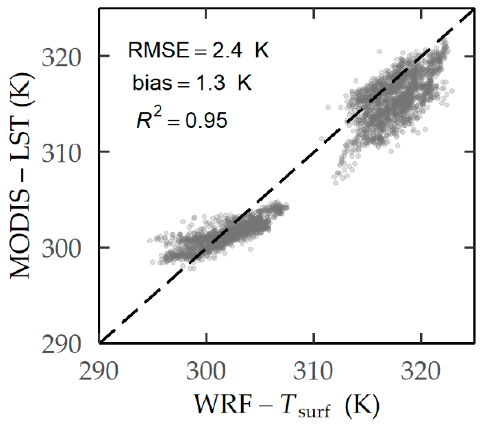
Next, the urban thermal climate of Athens was investigated using the WRF model for a five-day case-study (7–11 August 2017). The simulated surface temperature (T_s) was tested against cloud-free MODIS LST (Terra and Aqua) images. A reasonable agreement was found for the urban fabric—i.e., for the urban cells, λ_urb > 0—with an average RMSE = 2.4 K and a Mean Absolute Error (MAE) equal to 2.0 K. For the total study area—including the forested areas at the city boundaries—RMSE and MAE were 2.8 K and 2.3 K, respectively. However, as can be seen from Figure 12, the modeled surface temperature was generally systematically overestimated. The mean T_s–LST error (bias) was 1.3 K (2.0 K during daytime and 0.6 K at night). In addition, in the nighttime the highly vegetated neighborhoods (LCZ 5, 6, and 9) exhibited a slight to moderate underestimation of T_s (average bias = −0.4 K).

The above discrepancies can be better highlighted in the spatial mapping of T_s presented in Figure 13 (average model estimations compared against synchronous average LST values retrieved from MODIS Aqua). Nevertheless, despite the systematic differences, it can be observed that WRF–SLUCM was capable of matching to a fairly good extent the spatial patterns of satellite-derived LST.

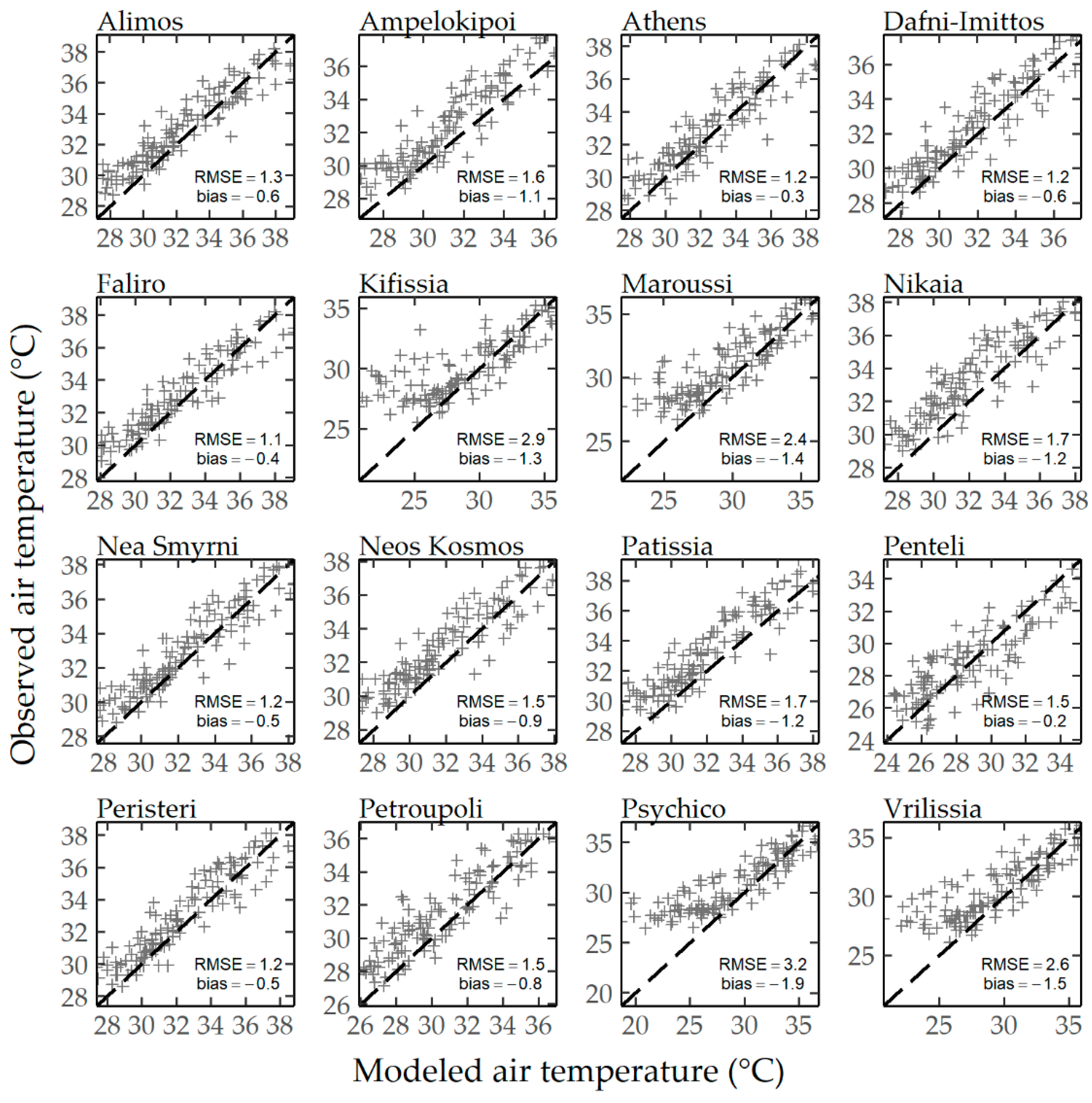
By day (Figure 13a) LCZ 8 (high λ_i and low H/W) was correctly simulated to have a higher surface temperature of ≈2 Κ compared to the neighboring densely built districts (LCZ 2₁ and LCZ 2). At night, the center of the open set LCZ 8 zone corresponded to a local minimum, 0.5–1 K cooler than the central areas with closely packed buildings (Figure 13b), in agreement to Aqua observations (Figure 13d). In addition, the model-observation comparison demonstrates that WRF noticeably captured the differentiation between the highly built-up and the heavily vegetated urban districts. However, the intra-urban variations were overestimated at nighttime because of the previously noted systematic errors. The evaluation of the model’s ability to predict the near-surface air temperature (T_as) is given in Figure 14. In general, WRF provided good estimates for the majority of the stations, with an RMSE varying from 1.2 to 3.2 Κ and an average value of 1.7 K. The larger errors were obtained for the less densely built-up LCZs as a result of significant underestimation of nocturnal T_as (average bias equal to −0.9 K for all stations). In addition to a general underestimation of the nocturnal thermal stress in well-vegetated urban areas that was also observed previously for T_s, the disagreement between modeled and observed values are considered to be further influenced by the location of the automatic meteorological stations. Specifically, while the majority of the stations are located within or near residential districts, modeled T_as corresponds to the aggregated temperature of both the impervious and the vegetated tile of the urban grid cell. 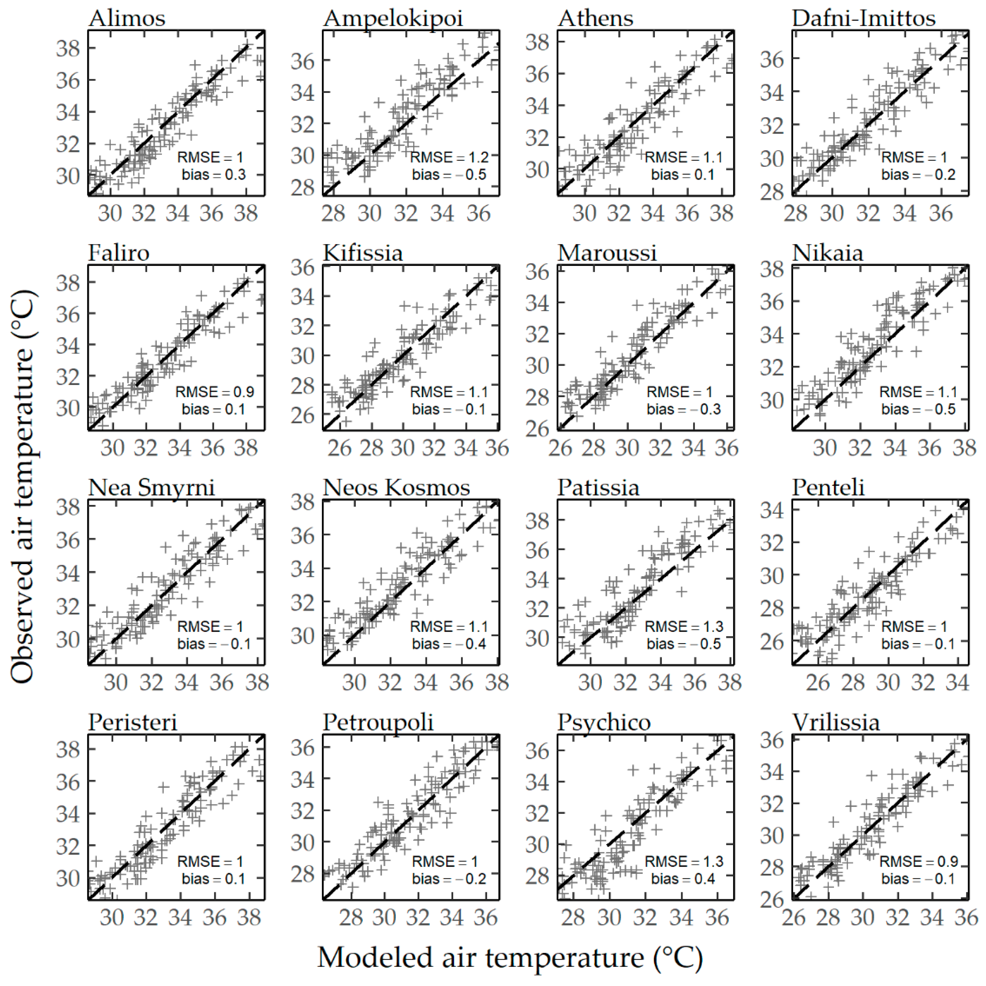Limiting the evaluation only to the impervious part of the modeled temperatures (T_as,urb), the negative bias was seen to consistently decrease (average bias = −0.1 K for all stations), while RMSE also became smaller, from 1.7 Κ to 1.1 Κ (Figure 15).

The considerably low bias using T_as,urb as a diagnostic output variable is reflected on the average modeled air temperature per LCZ for the total examined period (

Table 11. Average observed and modeled near-surface air temperature for the urban tile of the grid cell (T_as,urb) in Athens per LCZ (degrees Celsius) (7–11 August 2017).

	Daytime		Nighttime
	Station	Model	Station	Model
LCZ 21	34.1	33.8	31.3	30.8
LCZ 2	33.7	33.5	30.5	30.4
LCZ 3	34.5	34.0	31.6	31.1
LCZ 5	33.1	33.0	30.0	29.9
LCZ 6	31.8	31.8	28.5	28.8
LCZ 9	29.9	29.8	27.5	27.3

); results are divided into daytime (7 a.m. to 8 p.m. local time) and nighttime (9 p.m. to 7 a.m. local time) hours. It can be observed that the average thermal conditions for the different LCZs were well predicted. As expected, the less densely developed sites demonstrated lower average temperatures (also influenced by greater elevation). The variability among LCZs was observed to be relatively stable for daytime and nighttime estimates. 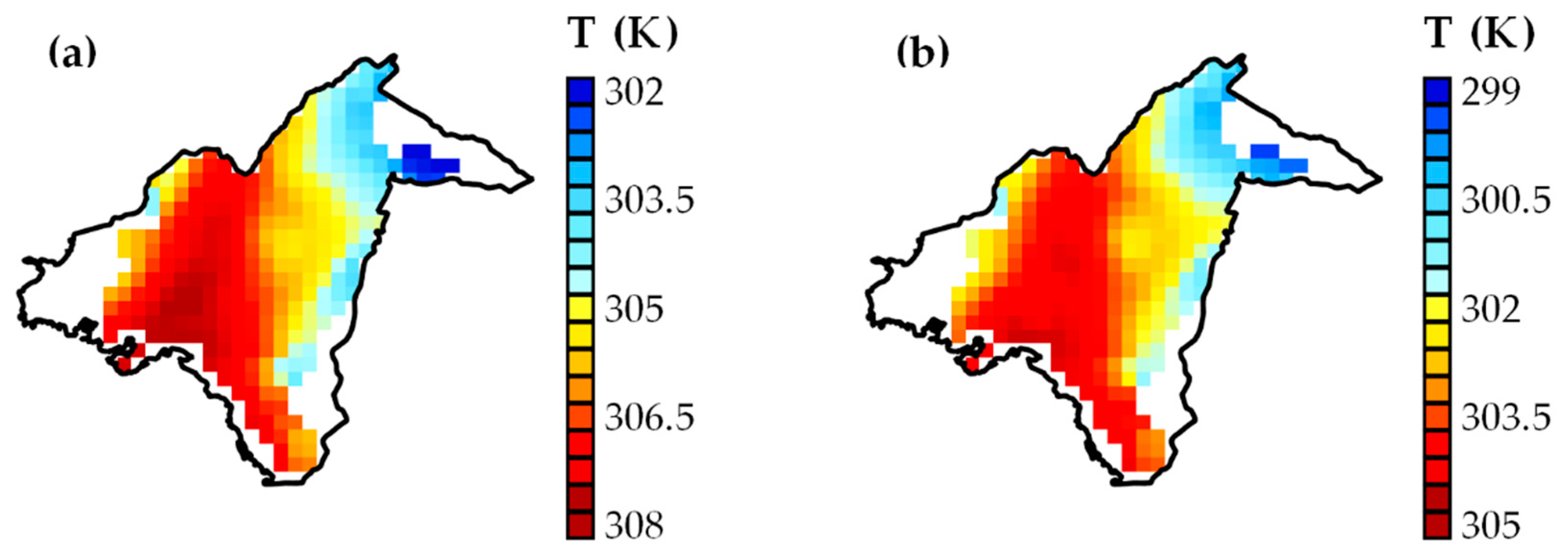Figure 16 gives the spatial distribution of the modeled near-surface, considering only the urban tile (T_as,urb). Similar to the surface temperature variability in Figure 8 and Figure 13, the closely packed LCZs of the broader center of Athens (LCZ 2₁ and LCZ 2) had a lower temperature in the order of 0.5 Κ than the adjacent LCZ 8 by day. At night, a difference of similar magnitude was observed, however, this time with higher T_as,urb for LCZ 2₁ and LCZ 2.

4. Discussion

Using statistical techniques, we assessed the relation between MODIS–LST and the surface parameters λ_imp, λ_b, and H for a total number of 25 European cities. Results revealed that λ_imp presented a clear and consistent positive influence on LST, as expected by previous studies [18,19,20]. This positive association was widespread across study areas also for the regression models. The main process responsible for the higher temperatures in the more heavily developed parts of a given city—controlling for further structure characteristics—can be attributed to decreased evapotranspirative losses.

By day, an exception to the general λ_imp–LST correlation was the lower-latitude cities—characterized by a particularly warm and dry summer climate, where λ_imp exhibited a weak positive or a negative bivariate relation to LST. This finding is consistent with the results of Imhoff et al. [19] for the arid and semi-arid cities in the United States, where part of inner-city areas were cooler than surrounding natural regions of lower λ_imp. This particular λ_imp–LST connection is considered to be a result of: (a) The properties of vegetation and soils in xeric biomes—lower moisture availability and subsequently decreased cooling effect and thermal admittance—and (b) the compact built-up structure and high thermal mass of the cities under consideration that leads to slower warming rates. When adjusting for λ_b and H with multiple regression models, there was also a positive effect of λ_imp on LST for the southern cities. This suggests that even when overall a negative daytime SUHI might be present, extended, open-set impervious areas (e.g., roads, parking lots) within the cities will typically be warmer than natural surfaces.

For λ_b and H, there was a large variability across cities with regard to their daytime relationship to LST. This is considered to be shaped by the various and contrasting effects that compact, high-rise urban design exerts on daytime microclimates. On the one hand, higher λ_b and H lead to increased absorption of short-wave radiation due to multiple reflections between canyon facets and to the stagnation of warm air within the urban canopy layer. On the other hand, closely spaced high-rise buildings increase the shading inside the canyon and especially on roads; as a result, solar radiation is reflected primarily at the rooftops, which generally have a higher albedo than canyon floors. Moreover, the increased size and number of active surfaces result in more heat being stored within the urban fabric. The prevailing characteristics and the range of values for λ_b and H of a given city result in a unique relationship for λ_b and H with LST as presented in Figure 5, Figure 6 and Figure 7 and Table 6.

The observed discrepancies between cities in this work are expected to be also influenced by the distinct ventilation potential that different districts have within a given city. Ventilation channels have been found to provide strong control over the thermal climate of a city, potentially alleviating the excess heat of urban form and function [107,108]. A more detailed analysis of the aerodynamic features [109,110] would be the goal of a future study in order to examine the importance of the proximity to wind corridors as a further determining parameter of the thermal environment.

Despite the differences across cities obtained in the current study, some general conclusions may be drawn from the statistical analysis: Regarding the bivariate correlation of λ_b and H with LST, a generally positive linkage was obtained, in agreement with previous works [37,43]. However, part of the above association is considered to be indirectly driven by the strong correlation that λ_b and H have with the impervious fraction (λ_imp). Adjusting for the influence of λ_imp using multiple linear regression, it was demonstrated that at a neighborhood scale (1000 m), closely spaced and tall buildings are not the driving factor of high daytime LST. In addition, it can be inferred that when wind shelter and canyon trapping are more than outweighed by increased shading and thermal admittance, densely urban areas tend to exhibit lower daytime LST than districts of similar λ_imp. In contrast, during nighttime, higher λ_b and H were generally associated—often strongly—with increasing LST, which can be attributed to reduced long-wave radiation loss. These findings were also consistent for the statistically significant results of the spatial regression models (SLM) (Table 8), giving further general support for the conclusions in this study.

More specifically with regard to the H–LST daytime relationship, it was found that for several cities, LST was decreasing with H (Table 6 and Table 7) and/or its maximum value was not obtained at the high-rise districts—especially for the heavily developed cities (e.g., Athens, London, Madrid, Paris, and Rome) (Figure 6). In this regard, previous statistical studies of the effect of H on daytime LST were conflicting: In some cities, H was considered to exert a positive control [37,39,43], whereas in other urban areas the control was negative [41,44,45,111]. The intercomparison of multiple cities in this work suggests that a single direction of influence cannot be generalized; however, generally, H resulted in a weak or negative contribution to high daytime LST. This study also supports previous qualitative findings observing that the high-rise urban core was not the warmer part of the city by day: In Vancouver [112], Paris [113], Shanghai [20], Phoenix [114], London [115], and Los Angeles [116]. Finally, in [117], it was demonstrated that in several cases worldwide, LCZ 1—corresponding to neighborhoods with the higher building heights—had lower LST compared to other LCZ classes with similar building density but lower height.

The discussion above highlights the importance of taking into account the diurnal course of surface temperature when evaluating the thermal environment of a city. Intra-urban differences in urban form provide control on the warming and cooling rates of different LCZs. However, as it has been noted in the literature [118], more than half of SUHI studies are limited to daytime thermal observations. As shown here, this can lead to a misidentification of the most thermally vulnerable locations of a city, in view of designing and implementing climate-sensitive mitigation responses of the urban heat island effect.

The accuracy of the LST retrieval in an urban environment using space-borne observations is affected by (a) the effects of atmospheric absorption, (b) the assignment of surface emissivity, and (c) the influence of thermal anisotropy. With regard to uncertainties in the atmospheric correction, it is considered that they have a negligible effect on the derived intra-urban variations since the study area extents under consideration were rather limited, therefore, atmospheric absorption between the surface and the sensor was more or less equally distributed across a given urban area.

Emissivity uncertainties in the MODIS–LST product (MOD/MYD11) are controlled by the accuracy of the land cover classification and the assumption that the assigned emissivity values of a given class are adequately representative [80]. Accuracy of MODIS emissivity is likely to affect primarily the λ_imp–LST relation, as MODIS classification does not consider urban structure differences. Conversely, the connection of H and LST is considered to be influenced by the urban geometry effect on the effective emissivity [119]. However, the consistent shift of regression coefficients for H obtained during daytime—weak positive or weak negative—and in nighttime—moderate/strong positive—suggest that the main part of urban structure control on LST is obtained independently of the emissivity retrieval.

As noted previously, one of the major findings in this work was the relatively lower LST in the daytime for the pixels (at 1000 m spatial resolution) with high H. The observed thermal radiation from satellite sensors is derived mostly by the rooftops and the road surface, as a result of the observing angle of the instrument. Adjusting the urban surface temperature for thermal anisotropy—i.e., considering in an indirect way the wall temperatures and using weights according to the relative fractions of canyon facets—would have potentially increased the resulting negative effect of H to LST by day, as thermal anisotropy increases with daytime H/W [120].

The connection between urban surface parameters and LST was further analyzed and interpreted in the urban area of Athens within the context of the LCZ scheme. As expected, the local climate zones with high vegetation density (LCZ 6 and LCZ 9) (i.e., low λ_imp values) tended to have the lower temperatures of the study area. By day, the large low-rise class (LCZ 8) yielded the higher LSTs, as a result of the increased impervious ground fraction (λ_i) (related to lower albedo and thermal admittance). The converse situation was observed at night, when the closely-spaced urban central areas (LCZ 2₁, LCZ 2, and LCZ 3) were warmer than LCZ 8, as for the latter, low H/W assists radiative cooling. Overall, the LCZ scheme was found to be valuable in assessing the major thermal patterns inside the urban area. Surface temperature differences among LCZs was consistent with previous related studies [111,117,121]. The more obvious distinction of LCZ 8 here during daytime is attributed to the extensive fractional coverage of this zone within the urban core of Athens, whereas the previously examined industrial sites in the literature have been mostly fragmented and/or on the outskirts of the city.

Using the meteorological model WRF together with a modified version of the urban parameterization scheme SLUCM, yielded an adequate agreement of the urban form controls on the thermal patterns in Athens. The systematic errors for LST were similar in magnitude with those reported in previous studies [55,63,97]. A part of the positive bias may be attributed to the slight underestimation of the reference MODIS product in Athens, as reported in [92]. The model to observation comparison of air temperatures showed a relatively low prediction error (RMSE = 1.7 K). However, a significant underestimation of nocturnal T_a was found for the stations in well-vegetated urban districts. Using only the modeled temperature for the impervious (urban) tile of the cells, the above systematic error reduced significantly. In addition to issues in relation to the location of the weather stations, the above discrepancies are considered to be associated with the tile approach of the default SLUCM scheme, whereby vegetation-buildings interactions are not incorporated. In future research it will be investigated how WRF modelled temperatures may be altered when vegetation-related processes can be directly included in the urban canyon (e.g., as in [97]), which is a key research focus for various currently developed urban parameterization schemes (e.g., [122]).

5. Conclusions

In this study, we assessed the influence of key urban surface parameters at the neighborhood scale (1000 m) thermal climate. The major conclusions for 25 European cities can be summarized as follows: The impervious urban fraction (λ_imp) had the most consistent and statistically significant relation to LST with a positive effect for the vast majority of the cities. By day, λ_b and H showed—after adjusting for λ_imp using regression analysis—either a weak positive or a negative influence on LST. Tall buildings, in particular, were commonly observed to contribute to a slight decrease in daytime surface temperature. The picture was altered during nighttime, where LST was mainly increasing for increasing λ_b and H (considering the statistically significant regression coefficients) with a similar magnitude to that of λ_imp. Moreover, the statistically significant results of spatial regression (SLM) were consistent with the multiple regression models. A more detailed investigation of the connection between urban structure and LST was conducted for Athens, using the LCZ scheme and additional surface parameters. For the urban core of the city a notable negative relation of LST with H/W and λ_c was estimated in the daytime (rho = −0.68 and −0.70, respectively), and in contrast, a positive association during nighttime (rho = 0.45 and 0.59, respectively). Results of a WRF numerical simulation for a 5-day period of high heat in Athens suggest that the model can reproduce the main spatial patterns of the urban area with an RMSE equal to 2.4 K for T_s and to 1.7 K for T_a; however, systematic underestimations were also present, especially for the heavily vegetated LCZs.

References

1. Oke, T.R. The energetic basis of the urban heat island. Q. J. R. Meteorol. Soc. 1982, 108, 1–24. [Google Scholar] [CrossRef]
2. Arnfield, A.J. Canyon geometry, the urban fabric and nocturnal cooling: A simulation approach. Phys. Geogr. 1990, 11, 220–239. [Google Scholar] [CrossRef]
3. Goward, S.N. Thermal Behavior of Urban Landscapes and the Urban Heat Island. Phys. Geogr. 1981, 2, 19–33. [Google Scholar] [CrossRef]
4. Oke, T.R. The urban energy balance. Prog. Phys. Geogr. Earth Environ. 1988, 12, 471–508. [Google Scholar] [CrossRef]
5. Aida, M. Urban albedo as a function of the urban structure—A model experiment. Bound. Layer Meteorol. 1982, 23, 405–413. [Google Scholar] [CrossRef]
6. Sailor, D.J. A review of methods for estimating anthropogenic heat and moisture emissions in the urban environment. Int. J. Climatol. 2011, 31, 189–199. [Google Scholar] [CrossRef]
7. Basu, R. High ambient temperature and mortality: A review of epidemiologic studies from 2001 to 2008. Environ. Health 2009, 8, 40. [Google Scholar] [CrossRef] [Green Version]
8. Santamouris, M.; Cartalis, C.; Synnefa, A.; Kolokotsa, D. On the impact of urban heat island and global warming on the power demand and electricity consumption of buildings—A review. Energy Build. 2015, 98, 119–124. [Google Scholar] [CrossRef]
9. Van Hove, L.W.A.; Jacobs, C.M.J.; Heusinkveld, B.G.; Elbers, J.A.; van Driel, B.L.; Holtslag, A.A.M. Temporal and spatial variability of urban heat island and thermal comfort within the Rotterdam agglomeration. Build. Environ. 2015, 83, 91–103. [Google Scholar] [CrossRef] [Green Version]
10. Pisello, A.L.; Saliari, M.; Vasilakopoulou, K.; Hadad, S.; Santamouris, M. Facing the urban overheating: Recent developments. Mitigation potential and sensitivity of the main technologies. Wiley Interdiscip. Rev. Energy Environ. 2018, 7, e294. [Google Scholar] [CrossRef]
11. Stewart, I.D.; Oke, T.R. Local Climate Zones for Urban Temperature Studies. Bull. Amer. Meteor. Soc. 2012, 93, 1879–1900. [Google Scholar] [CrossRef]
12. Stewart, I.D. A systematic review and scientific critique of methodology in modern urban heat island literature. Int. J. Climatol. 2011, 31, 200–217. [Google Scholar] [CrossRef]
13. Skarbit, N.; Stewart, I.D.; Unger, J.; Gál, T. Employing an urban meteorological network to monitor air temperature conditions in the ‘local climate zones’ of Szeged, Hungary. Int. J. Climatol. 2017, 37, 582–596. [Google Scholar] [CrossRef]
14. Voogt, J.A.; Oke, T.R. Thermal remote sensing of urban climates. Remote Sens. Environ. 2003, 86, 370–384. [Google Scholar] [CrossRef]
15. Azevedo, J.A.; Chapman, L.; Muller, C.L. Quantifying the Daytime and Night-Time Urban Heat Island in Birmingham, UK: A Comparison of Satellite Derived Land Surface Temperature and High Resolution Air Temperature Observations. Remote Sens. 2016, 8, 153. [Google Scholar] [CrossRef] [Green Version]
16. Gallo, K.P.; McNab, A.L.; Karl, T.R.; Brown, J.F.; Hood, J.J.; Tarpley, J.D. The use of a vegetation index for assessment of the urban heat island effect. Int. J. Remote Sens. 1993, 14, 2223–2230. [Google Scholar] [CrossRef]
17. Weng, Q.; Lu, D.; Schubring, J. Estimation of land surface temperature–vegetation abundance relationship for urban heat island studies. Remote Sens. Environ. 2004, 89, 467–483. [Google Scholar] [CrossRef]
18. Yuan, F.; Bauer, M.E. Comparison of impervious surface area and normalized difference vegetation index as indicators of surface urban heat island effects in Landsat imagery. Remote Sens. Environ. 2007, 106, 375–386. [Google Scholar] [CrossRef]
19. Imhoff, M.L.; Zhang, P.; Wolfe, R.E.; Bounoua, L. Remote sensing of the urban heat island effect across biomes in the continental USA. Remote Sens. Environ. 2010, 114, 504–513. [Google Scholar] [CrossRef] [Green Version]
20. Li, J.; Song, C.; Cao, L.; Zhu, F.; Meng, X.; Wu, J. Impacts of landscape structure on surface urban heat islands: A case study of Shanghai, China. Remote Sens. Environ. 2011, 115, 3249–3263. [Google Scholar] [CrossRef]
21. Zha, Y.; Gao, J.; Ni, S. Use of normalized difference built-up index in automatically mapping urban areas from TM imagery. Int. J. Remote Sens. 2003, 24, 583–594. [Google Scholar] [CrossRef]
22. Renard, F.; Alonso, L.; Fitts, Y.; Hadjiosif, A.; Comby, J. Evaluation of the Effect of Urban Redevelopment on Surface Urban Heat Islands. Remote Sens. 2019, 11, 299. [Google Scholar] [CrossRef] [Green Version]
23. Chen, X.-L.; Zhao, H.-M.; Li, P.-X.; Yin, Z.-Y. Remote sensing image-based analysis of the relationship between urban heat island and land use/cover changes. Remote Sens. Environ. 2006, 104, 133–146. [Google Scholar] [CrossRef]
24. Kawamura, M. Relation between social and environmental conditions in Colombo Sri Lanka and the urban index estimated by satellite remote sensing data. In Proceedings of the 51st Annual Conference of the Japan Society of Civil Engineers, Tokyo, Japan, 19–21 September 1996; pp. 190–191. [Google Scholar]
25. As-syakur, A.R.; Adnyana, I.W.S.; Arthana, I.W.; Nuarsa, I.W. Enhanced Built-Up and Bareness Index (EBBI) for Mapping Built-Up and Bare Land in an Urban Area. Remote Sens. 2012, 4, 2957–2970. [Google Scholar] [CrossRef] [Green Version]
26. Zhang, Y.; Chen, L.; Wang, Y.; Chen, L.; Yao, F.; Wu, P.; Wang, B.; Li, Y.; Zhou, T.; Zhang, T. Research on the Contribution of Urban Land Surface Moisture to the Alleviation Effect of Urban Land Surface Heat Based on Landsat 8 Data. Remote Sens. 2015, 7, 10737–10762. [Google Scholar] [CrossRef] [Green Version]
27. Zhou, W.; Huang, G.; Cadenasso, M.L. Does spatial configuration matter? Understanding the effects of land cover pattern on land surface temperature in urban landscapes. Landsc. Urban Plan. 2011, 102, 54–63. [Google Scholar] [CrossRef]
28. Connors, J.P.; Galletti, C.S.; Chow, W.T.L. Landscape configuration and urban heat island effects: Assessing the relationship between landscape characteristics and land surface temperature in Phoenix, Arizona. Landsc. Ecol. 2013, 28, 271–283. [Google Scholar] [CrossRef]
29. Ward, K.; Lauf, S.; Kleinschmit, B.; Endlicher, W. Heat waves and urban heat islands in Europe: A review of relevant drivers. Sci. Total Environ. 2016, 569–570, 527–539. [Google Scholar] [CrossRef]
30. Yue, W.; Liu, X.; Zhou, Y.; Liu, Y. Impacts of urban configuration on urban heat island: An empirical study in China mega-cities. Sci. Total Environ. 2019, 671, 1036–1046. [Google Scholar] [CrossRef]
31. Du, S.; Xiong, Z.; Wang, Y.-C.; Guo, L. Quantifying the multilevel effects of landscape composition and configuration on land surface temperature. Remote Sens. Environ. 2016, 178, 84–92. [Google Scholar] [CrossRef]
32. Chen, A.; Yao, L.; Sun, R.; Chen, L. How many metrics are required to identify the effects of the landscape pattern on land surface temperature? Ecol. Indic. 2014, 45, 424–433. [Google Scholar] [CrossRef]
33. Galletti, C.S.; Li, X.; Connors, J.P. Establishing the relationship between urban land-cover configuration and night time land-surface temperature using spatial regression. Int. J. Remote Sens. 2019, 40, 6752–6774. [Google Scholar] [CrossRef]
34. Nichol, J.E. High-Resolution Surface Temperature Patterns Related to Urban Morphology in a Tropical City: A Satellite-Based Study. J. Appl. Meteor. 1996, 35, 135–146. [Google Scholar] [CrossRef] [Green Version]
35. Xiao, R.; Weng, Q.; Ouyang, Z.; Li, W.; Schienke, E.W.; Zhang, Z. Land surface temperature variation and major factors in Beijing, China. Photogramm. Eng. Remote Sens. 2008, 74, 451–461. [Google Scholar] [CrossRef] [Green Version]
36. Wu, C.-D.; Lung, S.-C.C.; Jan, J.-F. Development of a 3-D urbanization index using digital terrain models for surface urban heat island effects. ISPRS J. Photogramm. Remote Sens. 2013, 81, 1–11. [Google Scholar] [CrossRef]
37. Berger, C.; Rosentreter, J.; Voltersen, M.; Baumgart, C.; Schmullius, C.; Hese, S. Spatio-temporal analysis of the relationship between 2D/3D urban site characteristics and land surface temperature. Remote Sens. Environ. 2017, 193, 225–243. [Google Scholar] [CrossRef]
38. Chun, B.; Guldmann, J.-M. Spatial statistical analysis and simulation of the urban heat island in high-density central cities. Landsc. Urban Plan. 2014, 125, 76–88. [Google Scholar] [CrossRef]
39. Guo, G.; Zhou, X.; Wu, Z.; Xiao, R.; Chen, Y. Characterizing the impact of urban morphology heterogeneity on land surface temperature in Guangzhou, China. Environ. Model. Softw. 2016, 84, 427–439. [Google Scholar] [CrossRef]
40. Chun, B.; Guhathakurta, S. Daytime and nighttime urban heat islands statistical models for Atlanta. Environ. Plan. B Urban Anal. City Sci. 2017, 44, 308–327. [Google Scholar] [CrossRef]
41. Cai, Z.; Han, G.; Chen, M. Do water bodies play an important role in the relationship between urban form and land surface temperature? Sustain. Cities Soc. 2018, 39, 487–498. [Google Scholar] [CrossRef]
42. Yin, C.; Yuan, M.; Lu, Y.; Huang, Y.; Liu, Y. Effects of urban form on the urban heat island effect based on spatial regression model. Sci. Total Environ. 2018, 634, 696–704. [Google Scholar] [CrossRef] [PubMed]
43. Yang, J.; Su, J.; Xia, J.; Jin, C.; Li, X.; Ge, Q. The Impact of Spatial Form of Urban Architecture on the Urban Thermal Environment: A Case Study of the Zhongshan District, Dalian, China. IEEE J. Sel. Top. Appl. Earth Obs. Remote Sens. 2018, 11, 2709–2716. [Google Scholar] [CrossRef]
44. Sun, Y.; Gao, C.; Li, J.; Wang, R.; Liu, J. Quantifying the Effects of Urban Form on Land Surface Temperature in Subtropical High-Density Urban Areas Using Machine Learning. Remote Sens. 2019, 11, 959. [Google Scholar] [CrossRef] [Green Version]
45. Zheng, Z.; Zhou, W.; Yan, J.; Qian, Y.; Wang, J.; Li, W. The higher, the cooler? Effects of building height on land surface temperatures in residential areas of Beijing. Phys. Chem. Earth Parts A/B/C 2019, 110, 149–156. [Google Scholar] [CrossRef]
46. Masson, V. A Physically-Based Scheme for the Urban Energy Budget in Atmospheric Models. Bound. Layer Meteorol. 2000, 94, 357–397. [Google Scholar] [CrossRef]
47. Kusaka, H.; Kondo, H.; Kikegawa, Y.; Kimura, F. A Simple Single-Layer Urban Canopy Model for Atmospheric Models: Comparison with Multi-Layer and Slab Models. Bound. Layer Meteorol. 2001, 101, 329–358. [Google Scholar] [CrossRef]
48. Dupont, S.; Otte, T.L.; Ching, J.K.S. Simulation of Meteorological Fields within and Above Urban and Rural Canopies with a Mesoscale Model. Bound. Layer Meteorol. 2004, 113, 111–158. [Google Scholar] [CrossRef]
49. Skamarock, W.C.; Klemp, J.B.; Dudhia, J.; Gill, D.O.; Barker, D.M.; Wang, W.; Powers, J.G. A Description of the Advanced Research WRF Version 3. NCAR Technical Note-475+ STR; National Center for Atmospheric Research: Boulder, CO, USA, 2008.
50. Chen, F.; Kusaka, H.; Bornstein, R.; Ching, J.; Grimmond, C.S.B.; Grossman-Clarke, S.; Loridan, T.; Manning, K.W.; Martilli, A.; Miao, S.; et al. The integrated WRF/urban modelling system: Development, evaluation, and applications to urban environmental problems. Int. J. Climatol. 2011, 31, 273–288. [Google Scholar] [CrossRef]
51. Liu, Y.; Chen, F.; Warner, T.; Basara, J. Verification of a Mesoscale Data-Assimilation and Forecasting System for the Oklahoma City Area during the Joint Urban 2003 Field Project. J. Appl. Meteor. Climatol. 2006, 45, 912–929. [Google Scholar] [CrossRef]
52. Kusaka, H.; Chen, F.; Bao, J.; Tewari, M.; Hirakuchi, H. Simulation of the urban heat island effects over the Greater Houston Area with the high resolution WRF/LSM/Urban coupled system. Simulation 2004, 1, 4. [Google Scholar]
53. Martilli, A.; Clappier, A.; Rotach, M.W. An Urban Surface Exchange Parameterisation for Mesoscale Models. Bound. Layer Meteorol. 2002, 104, 261–304. [Google Scholar] [CrossRef]
54. Salamanca, F.; Krpo, A.; Martilli, A.; Clappier, A. A new building energy model coupled with an urban canopy parameterization for urban climate simulations—Part I. formulation, verification, and sensitivity analysis of the model. Theor. Appl Clim. 2009, 99, 331. [Google Scholar] [CrossRef]
55. Giannaros, T.M.; Melas, D.; Daglis, I.A.; Keramitsoglou, I.; Kourtidis, K. Numerical study of the urban heat island over Athens (Greece) with the WRF model. Atmos. Environ. 2013, 73, 103–111. [Google Scholar] [CrossRef]
56. Li, D.; Bou-Zeid, E. Synergistic Interactions between Urban Heat Islands and Heat Waves: The Impact in Cities Is Larger than the Sum of Its Parts. J. Appl. Meteor. Climatol. 2013, 52, 2051–2064. [Google Scholar] [CrossRef] [Green Version]
57. Sarmiento, D.P.; Davis, K.J.; Deng, A.; Lauvaux, T.; Brewer, A.; Hardesty, M. A comprehensive assessment of land surface-atmosphere interactions in a WRF/Urban modeling system for Indianapolis, IN. Elem. Sci. Anth. 2017, 5, 23. [Google Scholar] [CrossRef] [Green Version]
58. Mauree, D.; Blond, N.; Clappier, A. Multi-scale modeling of the urban meteorology: Integration of a new canopy model in the WRF model. Urban Clim. 2018, 26, 60–75. [Google Scholar] [CrossRef] [Green Version]
59. Salamanca, F.; Zhang, Y.; Barlage, M.; Chen, F.; Mahalov, A.; Miao, S. Evaluation of the WRF-Urban Modeling System Coupled to Noah and Noah-MP Land Surface Models over a Semiarid Urban Environment. J. Geophys. Res. Atmos. 2018, 123, 2387–2408. [Google Scholar] [CrossRef]
60. Li, H.; Zhou, Y.; Wang, X.; Zhou, X.; Zhang, H.; Sodoudi, S. Quantifying urban heat island intensity and its physical mechanism using WRF/UCM. Sci. Total Environ. 2019, 650, 3110–3119. [Google Scholar] [CrossRef]
61. Ronda, R.J.; Steeneveld, G.J.; Heusinkveld, B.G.; Attema, J.J.; Holtslag, A.A.M. Urban Finescale Forecasting Reveals Weather Conditions with Unprecedented Detail. Bull. Am. Meteorol. Soc. 2017, 98, 2675–2688. [Google Scholar] [CrossRef]
62. Vahmani, P.; Ban-Weiss, G.A. Impact of remotely sensed albedo and vegetation fraction on simulation of urban climate in WRF-urban canopy model: A case study of the urban heat island in Los Angeles. J. Geophys. Res. Atmos. 2016, 121, 1511–1531. [Google Scholar] [CrossRef]
63. Göndöcs, J.; Breuer, H.; Pongrácz, R.; Bartholy, J. Urban heat island mesoscale modelling study for the Budapest agglomeration area using the WRF model. Urban Clim. 2017, 21, 66–86. [Google Scholar] [CrossRef]
64. Giannaros, C.; Nenes, A.; Giannaros, T.M.; Kourtidis, K.; Melas, D. A comprehensive approach for the simulation of the Urban Heat Island effect with the WRF/SLUCM modeling system: The case of Athens (Greece). Atmos. Res. 2018, 201, 86–101. [Google Scholar] [CrossRef]
65. Mills, G.; Ching, J.; See, L.; Bechtel, B.; Foley, M. An Introduction to the WUDAPT project. In Proceedings of the 9th International Conference on Urban Climate, Toulouse, France, 20–24 July 2015; pp. 20–24. [Google Scholar]
66. Brousse, O.; Martilli, A.; Foley, M.; Mills, G.; Bechtel, B. WUDAPT, an efficient land use producing data tool for mesoscale models? Integration of urban LCZ in WRF over Madrid. Urban Clim. 2016, 17, 116–134. [Google Scholar] [CrossRef]
67. Hammerberg, K.; Brousse, O.; Martilli, A.; Mahdavi, A. Implications of employing detailed urban canopy parameters for mesoscale climate modelling: A comparison between WUDAPT and GIS databases over Vienna, Austria. Int. J. Climatol. 2018, 38, e1241–e1257. [Google Scholar] [CrossRef] [Green Version]
68. Franco, D.M.P.; de Fatima Andrade, M.; Ynoue, R.Y.; Ching, J. Effect of Local Climate Zone (LCZ) classification on ozone chemical transport model simulations in Sao Paulo, Brazil. Urban Clim. 2019, 27, 293–313. [Google Scholar] [CrossRef]
69. Kwok, Y.T.; Schoetter, R.; Lau, K.K.-L.; Hidalgo, J.; Ren, C.; Pigeon, G.; Masson, V. How well does the local climate zone scheme discern the thermal environment of Toulouse (France)? An analysis using numerical simulation data. Int. J. Climatol. 2019, 39, 5292–5315. [Google Scholar] [CrossRef]
70. Molnár, G.; Gyöngyösi, A.Z.; Gál, T. Integration of an LCZ-based classification into WRF to assess the intra-urban temperature pattern under a heatwave period in Szeged, Hungary. Appl Clim. 2019, 138, 1139–1158. [Google Scholar] [CrossRef] [Green Version]
71. Kottek, M.; Grieser, J.; Beck, C.; Rudolf, B.; Rubel, F. World map of the Köppen-Geiger climate classification updated. Meteorol. Z. 2006, 15, 259–263. [Google Scholar] [CrossRef]
72. Fouillet, A.; Rey, G.; Laurent, F.; Pavillon, G.; Bellec, S.; Guihenneuc-Jouyaux, C.; Clavel, J.; Jougla, E.; Hémon, D. Excess mortality related to the August 2003 heat wave in France. Int. Arch. Occup. Environ. Health 2006, 80, 16–24. [Google Scholar] [CrossRef] [Green Version]
73. Guerreiro, S.B.; Dawson, R.J.; Kilsby, C.; Lewis, E.; Ford, A. Future heat-waves, droughts and floods in 571 European cities. Environ. Res. Lett. 2018, 13, 034009. [Google Scholar] [CrossRef]
74. Hellenic Statistical Authority (ELSTAT). 2011 Population-Housing Census. Available online: http://www.statistics.gr/en/2011-census-pop-hous (accessed on 9 February 2019).
75. Giannopoulou, K.; Livada, I.; Santamouris, M.; Saliari, M.; Assimakopoulos, M.; Caouris, Y.G. On the characteristics of the summer urban heat island in Athens, Greece. Sustain. Cities Soc. 2011, 1, 16–28. [Google Scholar] [CrossRef]
76. Kourtidis, K.; Georgoulias, A.K.; Rapsomanikis, S.; Amiridis, V.; Keramitsoglou, I.; Hooyberghs, H.; Maiheu, B.; Melas, D. A study of the hourly variability of the urban heat island effect in the Greater Athens Area during summer. Sci. Total Environ. 2015, 517, 162–177. [Google Scholar] [CrossRef] [Green Version]
77. United Nations, Department of Economic and Social Affairs. Population Division. Revision of World Urbanization Prospects. 2018. Available online: https://population.un.org/wup (accessed on 30 May 2020).
78. Agathangelidis, I.; Cartalis, C.; Santamouris, M. Integrating Urban Form, Function, and Energy Fluxes in a Heat Exposure Indicator in View of Intra-Urban Heat Island Assessment and Climate Change Adaptation. Climate 2019, 7, 75. [Google Scholar] [CrossRef] [Green Version]
79. Wan, Z. New refinements and validation of the collection-6 MODIS land-surface temperature/emissivity product. Remote Sens. Environ. 2014, 140, 36–45. [Google Scholar] [CrossRef]
80. Duan, S.-B.; Li, Z.-L.; Li, H.; Göttsche, F.-M.; Wu, H.; Zhao, W.; Leng, P.; Zhang, X.; Coll, C. Validation of Collection 6 MODIS land surface temperature product using in situ measurements. Remote Sens. Environ. 2019, 225, 16–29. [Google Scholar] [CrossRef] [Green Version]
81. Cleveland, W.S. Robust locally weighted regression and smoothing scatterplots. J. Am. Stat. Assoc. 1979, 74, 829–836. [Google Scholar] [CrossRef]
82. Alin, A. Multicollinearity. Wiley Interdiscip. Rev. Comput. Stat. 2010, 2, 370–374. [Google Scholar] [CrossRef]
83. Anselin, L. Lagrange Multiplier Test Diagnostics for Spatial Dependence and Spatial Heterogeneity. Geogr. Anal. 1988, 20, 1–17. [Google Scholar] [CrossRef]
84. Hong, S.-Y.; Lim, J.-O.J. The WRF single-moment 6-class microphysics scheme (WSM6). Asia Pac. J. Atmos. Sci. 2006, 42, 129–151. [Google Scholar]
85. Kain, J.S. The Kain–Fritsch convective parameterization: An update. J. Appl. Meteorol. 2004, 43, 170–181. [Google Scholar] [CrossRef] [Green Version]
86. Dudhia, J. Numerical study of convection observed during the winter monsoon experiment using a mesoscale two-dimensional model. J. Atmos. Sci. 1989, 46, 3077–3107. [Google Scholar] [CrossRef]
87. Mlawer, E.J.; Taubman, S.J.; Brown, P.D.; Iacono, M.J.; Clough, S.A. Radiative transfer for inhomogeneous atmospheres: RRTM, a validated correlated-k model for the longwave. J. Geophys. Res. Atmos. 1997, 102, 16663–16682. [Google Scholar] [CrossRef] [Green Version]
88. Hong, S.-Y.; Noh, Y.; Dudhia, J. A new vertical diffusion package with an explicit treatment of entrainment processes. Mon. Weather Rev. 2006, 134, 2318–2341. [Google Scholar] [CrossRef] [Green Version]
89. Paulson, C.A. The mathematical representation of wind speed and temperature profiles in the unstable atmospheric surface layer. J. Appl. Meteorol. 1970, 9, 857–861. [Google Scholar] [CrossRef]
90. Chen, F.; Dudhia, J. Coupling an advanced land surface–hydrology model with the Penn State–NCAR MM5 modeling system. Part I: Model implementation and sensitivity. Mon. Weather Rev. 2001, 129, 569–585. [Google Scholar] [CrossRef] [Green Version]
91. Friedl, M.A.; Sulla-Menashe, D.; Tan, B.; Schneider, A.; Ramankutty, N.; Sibley, A.; Huang, X. MODIS Collection 5 global land cover: Algorithm refinements and characterization of new datasets. Remote Sens. Environ. 2010, 114, 168–182. [Google Scholar] [CrossRef]
92. Agathangelidis, I.; Cartalis, C. Improving the disaggregation of MODIS land surface temperatures in an urban environment: A statistical downscaling approach using high-resolution emissivity. Int. J. Remote Sens. 2019, 40, 5261–5286. [Google Scholar] [CrossRef]
93. Baldridge, A.; Hook, S.; Grove, C.; Rivera, G. The ASTER spectral library version 2.0. Remote Sens. Environ. 2009, 113, 711–715. [Google Scholar] [CrossRef]
94. Kotthaus, S.; Smith, T.E.L.; Wooster, M.J.; Grimmond, C.S.B. Derivation of an urban materials spectral library through emittance and reflectance spectroscopy. ISPRS J. Photogramm. Remote Sens. 2014, 94, 194–212. [Google Scholar] [CrossRef] [Green Version]
95. Papamanolis, N. The main characteristics of the urban climate and the air quality in Greek cities. Urban Clim. 2015, 12, 49–64. [Google Scholar] [CrossRef]
96. Oke, T.R.; Mills, G.; Christen, A.; Voogt, J.A. Urban Climates; Cambridge University Press: Cambridge, UK, 2017. [Google Scholar]
97. Li, D.; Bou-Zeid, E. Quality and sensitivity of high-resolution numerical simulation of urban heat islands. Environ. Res. Lett. 2014, 9, 055001. [Google Scholar] [CrossRef]
98. Kanda, M.; Kanega, M.; Kawai, T.; Moriwaki, R.; Sugawara, H. Roughness Lengths for Momentum and Heat Derived from Outdoor Urban Scale Models. J. Appl. Meteor. Climatol. 2007, 46, 1067–1079. [Google Scholar] [CrossRef]
99. Trusilova, K.; Früh, B.; Brienen, S.; Walter, A.; Masson, V.; Pigeon, G.; Becker, P. Implementation of an Urban Parameterization Scheme into the Regional Climate Model COSMO-CLM. J. Appl. Meteor. Climatol. 2013, 52, 2296–2311. [Google Scholar] [CrossRef]
100. Lagouvardos, K.; Kotroni, V.; Bezes, A.; Koletsis, I.; Kopania, T.; Lykoudis, S.; Mazarakis, N.; Papagiannaki, K.; Vougioukas, S. The automatic weather stations NOANN network of the National Observatory of Athens: Operation and database. Geosci. Data J. 2017, 4, 4–16. [Google Scholar] [CrossRef]
101. Founda, D.; Santamouris, M. Synergies between Urban Heat Island and Heat Waves in Athens (Greece), during an extremely hot summer (2012). Sci. Rep. 2017, 7, 10973. [Google Scholar] [CrossRef] [PubMed] [Green Version]
102. Kolokotsa, D.; Psomas, A.; Karapidakis, E. Urban heat island in southern Europe: The case study of Hania, Crete. Sol. Energy 2009, 83, 1871–1883. [Google Scholar] [CrossRef]
103. Khan, H.S.; Paolini, R.; Santamouris, M.; Caccetta, P. Exploring the Synergies between Urban Overheating and Heatwaves (HWs) in Western Sydney. Energies 2020, 13, 470. [Google Scholar] [CrossRef] [Green Version]
104. LeSage, J.; Pace, R.K. Introduction to Spatial Econometrics; Chapman and Hall/CRC: Boca Raton, FL, USA, 2009. [Google Scholar]
105. Mills, G. Cities as agents of global change. Int. J. Climatol. 2007, 27, 1849–1857. [Google Scholar] [CrossRef]
106. Prezerakos, N.G. Characteristics of the sea breeze in Attica, Greece. Bound. Layer Meteorol. 1986, 36, 245–266. [Google Scholar] [CrossRef]
107. Suder, A.; Szymanowski, M. Determination of Ventilation Channels In Urban Area: A Case Study of Wrocław (Poland). Pure Appl. Geophys. 2014, 171, 965–975. [Google Scholar] [CrossRef] [Green Version]
108. Yang, J.; Jin, S.; Xiao, X.; Jin, C.; Xia, J.C.; Li, X.; Wang, S. Local climate zone ventilation and urban land surface temperatures: Towards a performance-based and wind-sensitive planning proposal in megacities. Sustain. Cities Soc. 2019, 47, 101487. [Google Scholar] [CrossRef]
109. Gál, T.; Unger, J. Detection of ventilation paths using high-resolution roughness parameter mapping in a large urban area. Build. Environ. 2009, 44, 198–206. [Google Scholar] [CrossRef]
110. Hsieh, C.-M.; Huang, H.-C. Mitigating urban heat islands: A method to identify potential wind corridor for cooling and ventilation. Comput. Environ. Urban Syst. 2016, 57, 130–143. [Google Scholar] [CrossRef]
111. Quan, J. Multi-Temporal Effects of Urban Forms and Functions on Urban Heat Islands Based on Local Climate Zone Classification. Int. J. Environ. Res. Public Health 2019, 16, 2140. [Google Scholar] [CrossRef] [Green Version]
112. Roth, M.; Oke, T.; Emery, W. Satellite-derived urban heat islands from three coastal cities and the utilization of such data in urban climatology. Int. J. Remote Sens. 1989, 10, 1699–1720. [Google Scholar] [CrossRef]
113. Dousset, B.; Gourmelon, F.; Laaidi, K.; Zeghnoun, A.; Giraudet, E.; Bretin, P.; Mauri, E.; Vandentorren, S. Satellite monitoring of summer heat waves in the Paris metropolitan area. Int. J. Climatol. 2011, 31, 313–323. [Google Scholar] [CrossRef]
114. Myint, S.W.; Wentz, E.A.; Brazel, A.J.; Quattrochi, D.A. The impact of distinct anthropogenic and vegetation features on urban warming. Landsc. Ecol. 2013, 28, 959–978. [Google Scholar] [CrossRef] [Green Version]
115. Crawford, B.; Grimmond, S.B.; Gabey, A.; Marconcini, M.; Ward, H.C.; Kent, C.W. Variability of urban surface temperatures and implications for aerodynamic energy exchange in unstable conditions. Q. J. R. Meteorol. Soc. 2018, 144, 1719–1741. [Google Scholar] [CrossRef]
116. Hulley, G.; Shivers, S.; Wetherley, E.; Cudd, R. New ECOSTRESS and MODIS Land Surface Temperature Data Reveal Fine-Scale Heat Vulnerability in Cities: A Case Study for Los Angeles County, California. Remote Sens. 2019, 11, 2136. [Google Scholar] [CrossRef] [Green Version]
117. Bechtel, B.; Demuzere, M.; Mills, G.; Zhan, W.; Sismanidis, P.; Small, C.; Voogt, J. SUHI analysis using Local Climate Zones—A comparison of 50 cities. Urban Clim. 2019, 28, 100451. [Google Scholar] [CrossRef]
118. Zhou, D.; Xiao, J.; Bonafoni, S.; Berger, C.; Deilami, K.; Zhou, Y.; Frolking, S.; Yao, R.; Qiao, Z.; Sobrino, J.A. Satellite Remote Sensing of Surface Urban Heat Islands: Progress, Challenges, and Perspectives. Remote Sens. 2019, 11, 48. [Google Scholar] [CrossRef] [Green Version]
119. Yang, J.; Wong, M.S.; Menenti, M.; Nichol, J. Modeling the effective emissivity of the urban canopy using sky view factor. ISPRS J. Photogramm. Remote Sens. 2015, 105, 211–219. [Google Scholar] [CrossRef]
120. Krayenhoff, E.S.; Voogt, J.A. Daytime Thermal Anisotropy of Urban Neighbourhoods: Morphological Causation. Remote Sens. 2016, 8, 108. [Google Scholar] [CrossRef] [Green Version]
121. Geletič, J.; Lehnert, M.; Dobrovolný, P. Land Surface Temperature Differences within Local Climate Zones, Based on Two Central European Cities. Remote Sens. 2016, 8, 788. [Google Scholar] [CrossRef] [Green Version]
122. Nice, K.A.; Coutts, A.M.; Tapper, N.J. Development of the VTUF-3D v1.0 urban micro-climate model to support assessment of urban vegetation influences on human thermal comfort. Urban Clim. 2018, 24, 1052–1076. [Google Scholar] [CrossRef] [Green Version]
Figure 1. Location of the 25 European cities used in this study. Dashed lines indicate the Weather Research and Forecasting (WRF) simulation domains; ascending order from the lower (D1) to the higher resolution domain (D4).
Climate 08 00131 g001
Figure 2. Study domain of Athens and the location of the meteorological stations used in this study; the station codes are given in Section 2.4. Base map: Landsat 8 Operational Land Imager (OLI), true color composite image for 28 June 2017.
Climate 08 00131 g002
Figure 3. Spatial distribution of the surface parameters in Athens at 1 km resolution: (a) λimp, (b) λb, (c) H, (d) H/W, (e) λc, and (f) λi.
Climate 08 00131 g003
Figure 4. Mapping of the Local Climate Zones (LCZs) in Athens at 1 km resolution.
Climate 08 00131 g004
Figure 5. The relationship between LST λimp, λb, and H for all cities combined: During daytime (ac), and during nighttime (df). Black curves correspond to the lowess regression lines. Blue lines and R2 correspond to the linear regression fit.
Climate 08 00131 g005
Figure 6. The relationship between LST and H for all cities during daytime. Black curves correspond to the lowess regression lines. Blue lines and R2 correspond to the linear regression fit.
Climate 08 00131 g006
Figure 7. As in Figure 6, during nighttime.
Climate 08 00131 g007
Figure 8. Spatial distribution of the average MODIS–LST (AQUA) in Athens for June–August 2017, (a) ≈14.30 local time and (b) ≈02.30 local time.
Climate 08 00131 g008
Figure 9. As in Figure 8, showing the isopleths of the difference to the average LST of the total study area, (a) ≈14.30 local time and (b) ≈02.30 local time.
Climate 08 00131 g009
Figure 10. The relationship between H/W, λc, and λi for the urban area of Athens: During daytime (ac), and during nighttime (df). Black curves correspond to the lowess regression lines. Blue lines and R2 correspond to the linear regression fit.
Climate 08 00131 g010
Figure 11. As in Figure 10, for the urban core of Athens (as defined in Figure 2). During daytime (ac), and during nighttime (df).
Climate 08 00131 g011
Figure 12. Comparison of the observed MODIS–LST (Aqua and Terra) and modeled surface temperature from WRF (Ts) (average for the available imagery in 7–11 August 2017).
Climate 08 00131 g012
Figure 13. Spatial distribution of the modeled surface temperature in Athens using WRF (Ts) and of MODIS–LST (Aqua) (average for the available imagery in 7–11 August 2017) during daytime (a) and (c) (≈14.30 local time), and during nighttime (b) and (d) ≈02.30 local time, respectively.
Climate 08 00131 g013
Figure 14. Comparison of the observed near-surface air temperature and the modeled near-surface air temperature from WRF (diagnostic variable Tas) (7–11 August 2017).
Climate 08 00131 g014
Figure 15. As in Figure 14, for the diagnostic variable Tas,urb.
Climate 08 00131 g015
Figure 16. Spatial distribution of the modeled near-surface temperature in Athens using WRF (diagnostic variable Tas) (7–11 August 2017), during daytime (a) and during nighttime (b).
Climate 08 00131 g016