Modeling the Impacts of Climate Change on Crop Yield and Irrigation in the Monocacy River Watershed, USA

Abstract

Crop yield depends on multiple factors, including climate conditions, soil characteristics, and available water. The objective of this study was to evaluate the impact of projected temperature and precipitation changes on crop yields in the Monocacy River Watershed in the Mid-Atlantic United States based on climate change scenarios. The Soil and Water Assessment Tool (SWAT) was applied to simulate watershed hydrology and crop yield. To evaluate the effect of future climate projections, four global climate models (GCMs) and three representative concentration pathways (RCP 4.5, 6, and 8.5) were used in the SWAT model. According to all GCMs and RCPs, a warmer climate with a wetter Autumn and Spring and a drier late Summer season is anticipated by mid and late century in this region. To evaluate future management strategies, water budget and crop yields were assessed for two scenarios: current rainfed and adaptive irrigated conditions. Irrigation would improve corn yields during mid-century across all scenarios. However, prolonged irrigation would have a negative impact due to nutrients runoff on both corn and soybean yields compared to rainfed condition. Decision tree analysis indicated that corn and soybean yields are most influenced by soil moisture, temperature, and precipitation as well as the water management practice used (i.e., rainfed or irrigated). The computed values from the SWAT modeling can be used as guidelines for water resource managers in this watershed to plan for projected water shortages and manage crop yields based on projected climate change conditions.

1. Introduction

Water budgets and crop production are affected by climate variability and change, including rising temperatures, less snowpack, and changing precipitation patterns [1,2,3,4]. There is evidence that natural systems in all continents and most oceans are being affected by regional climate change, with measured increases in temperature and atmospheric carbon dioxide (CO₂) [5]. Ongoing changes and increases in water demand can have significant effects on anthropogenic water demand water demand by vegetation, water availability, water stress, and, thus, crop yield [3,6,7]. Projected changes in seasonal variations in temperature and precipitation patterns and increasing greenhouse gases are expected to strongly affect hydrological (water budget) and agroecosystem (crop production) processes [3,6,8].

The impact of climate change on agricultural production varies through space and time, with positive impacts in some agricultural systems and regions and negative impacts in others [9,10]. For example, in Northern Europe, temperature increases are expected to reduce grain yields of cereals due to shortening of the grain filling period, while the combined effect of climate change is predicted to be beneficial in other regions, such as Canada [11]. For moderate changes in climate, the adverse effects of increased temperature on grain yields are expected to be offset by increased CO₂ concentrations [11]. A study by Goldblum [12] in Illinois, USA concluded that corn and soybean yields would decline under the variable future climate conditions, with a negative correlation between monthly temperature and yields. Overall, it is expected that future climate changes are likely to improve crop productivity in some areas and diminish it in others. It is important to assess the impact of climate changes on future water resources in order to evaluate the adaptive agricultural management needed to maintain expected crop productivity [13].

In the Mid-Atlantic USA, scientists have predicted a wide range of climate change-induced effects, including changes in agricultural and forest production, degraded fisheries, and the influx of invasive plants [14]. The Intergovernmental Panel on Climate Change (IPCC) estimated that by year 2100, the average temperatures in the Mid-Atlantic might increase by 1.34 to 5.78 °C compared to baseline conditions, while summer precipitation is expected to decrease compared to baseline conditions [15]. In addition, rapid population growth and development in this region will likely increase the risk of water insecurity and affect agricultural production. It is predicted that, by year 2040, the Mid-Atlantic region might experience medium to high water stress driven by high water demand [16]. The water permit database in the Mid-Atlantic state of Maryland indicated that seasonal variability is driving more irrigation withdrawals to meet increased crop water demand. For proper water resource management, regional water resource managers need information on the projected changes in water demand in response to future climate change.

It is important for researchers, policymakers, and water resource managers to understand watershed scale hydrological processes to estimate forthcoming water stress and crop water demand. Researchers estimated water stress and crop productivity under different climate change conditions using both field experiments and modeling [13,17,18]. Researchers have evaluated the impacts of climate change on watershed hydrology and crop yield under existing management practices [19] or the effects of different irrigation conditions, such as irrigation amounts [20], timing, and frequency [21]. Very few studies have evaluated the benefits of adaptive irrigation conditions over existing rainfed conditions from field-scale experiments [22] to regional scale modeling approaches [21] for limited climate change scenarios. To the best of our knowledge, no study has evaluated watershed scale effectiveness of adaptive irrigation strategies on existing rainfed conditions for a broad range of plausible climate change scenarios.

To address this knowledge gap, we conducted a holistic investigation of Mid-Atlantic USA water resources to determine the impacts of climate change on different components of water balance and crop yield. The Monocacy River Watershed was selected as a representation of the Mid-Atlantic USA, and the hydrologic model was developed for this watershed. The use of hydrologic models in planning and management of water resources and analyzing the impact of climate change on water components has become more important and common. Using hydrologic model, managers can choose effective measures and implement adaptive management strategies to overcome a wide range of plausible future conditions and events. The main objectives of this study were:

(1)

to assess the impact of future climate changes on watershed hydrology;

(2)

to investigate the impact of future climate changes on crop yields;

(3)

to evaluate the effects of irrigation as an adaptive strategy on crop yields; and

(4)

to identify the potential hydrological components that influence the crop yields.

2. Materials and Methods

2.1. Study Area

The Monocacy River Watershed is in the northeast Potomac River basin and extends to parts of Adams County in Pennsylvania and Frederick and Carroll Counties in Maryland, USA (Figure 1). The Monocacy River is the largest Maryland tributary to the Potomac River, and agriculture is the major land use in this watershed. According to the 2018 United States Department of Agriculture’s (USDA) Crop Data Layer [23], the Monocacy River Watershed is dominated by agricultural land (51.1%), followed by forested (36.2%) and urban areas (12.1%). Within this watershed, the most prominent croplands are corn (13.1%) and soybeans (10.8%) (

Table 1. Land use and land cover in the Monocacy River Watershed based on 2018 Crop Data Layer.

Land Use/Cover	Area (acres)	Area (km2)	Watershed Area (%)
Forest	189,307.88	766.10	36.24
Agricultural Land	268,109.67	1085.06	51.33
Urban Area	68,957.65	255.12	12.07
Grassland	1243.05	5.03	0.24
Water	662.31	2.68	0.13
Agricultural Land	Area (acres)	Area (km2)	Watershed Area (%)
Hay	75,540.25	305.70	14.46
Corn	68,321.40	276.49	13.08
Pasture	58,279.52	235.85	11.16
Soybean	56,368.50	228.12	10.79
Winter Wheat	8315.58	33.65	1.59
Alfalfa	935.82	3.79	0.18
Apple	362.05	1.47	0.07

). The average temperature in the region is 24 °C during the summer and 3 °C during the winter [24]. The average annual precipitation is 1105 mm, with monthly averages ranging from 64 to 115 mm. Snow accumulation occurs mainly in January, February, and March.

The prominent sources of water for crop production are groundwater and rainfall. A dense network of streams drains the water through the watershed, and fractured bedrock aquifers underlie this basin, which continually discharges groundwater into streams to sustain healthy aquatic ecosystems [25]. Groundwater is stored in interconnected fractures of bedrock aquifer and drains the basin rapidly due to minimal primary porosity and permeability; therefore, future drought (winter or summer) could negatively impact both water resources (groundwater and surface water) and crop yields. As with most watersheds in the Mid-Atlantic, the hydrology of the Monocacy River Watershed, with its stream/aquifer system, is highly seasonal. The recharge period for the watershed’s aquifer is late fall and winter, and both aquifer levels and stream flows tend to be highest during the wintertime and lowest in the summertime due to high evapotranspiration rates [25]. In this region, water availability problems typically occur in late summer and early fall (July, August, and September) [25].

2.2. Hydrologic Model

In this study, the Soil and Water Assessment Tool (SWAT) [26], which is a physically-based, semi-distributed, hydraulic model, was used to quantify the impact of climate change on the hydrology and the crop production of the Monocacy River Watershed. In a semi-distributed model, a watershed is broken down into smaller sub-basins, and a hydrologic system is estimated based on physically based algorithms. Runoff amounts from methods such as unit hydrograph are used to estimate streamflow from each of these sub-basins. SWAT was developed to evaluate the impact of climate and land management practices on watershed hydrology in large and complex watersheds over long periods of time [27]. Worldwide, the SWAT model has been used to analyze the effects of climate change scenarios on current watershed conditions and crop production [18,28,29]. Researchers have previously applied the SWAT model to investigate adaptive management practices to mitigate climate change-induced alterations [6,30].

During model development, the watershed was divided into a number of sub-basins and categorized into hydrological response units based on homogeneous soil types, land-use types, and slope classes, allowing for a high level of spatially detailed simulations. The SWAT model uses a water balance equation (see Equation (1)) to estimate the different water balance components of water resources (e.g., blue and green waters) at both the subbasin and the hydrological response unit level [26,27,31]. Blue water includes water flows through or below the land surface and stored in lakes, reservoirs, and aquifers, and green water includes the portion of precipitation that infiltrates and is stored as soil water storage and then returns to the atmosphere via transpiration and evaporation.

$$S{W}_t={\mathrm{SW}}_0+{\displaystyle \sum }_{n=i}^t(\mathrm{P}-Q_{surf}-\mathrm{ET}-w_{seep}-Q_{gw})$$

(1)

where SW_t and SW₀ are the changes in soil water storage at times t and 0, P is precipitation, Q_surf is surface runoff flow, ET is evapotranspiration, w_seep is aquifer recharge, and Q_gw is groundwater flow.

For the water budget, the SWAT model differentiates between solid and liquid precipitation based on near-surface air temperature. If the air temperature is lower than the snowfall temperature, then the precipitation is considered solid, i.e., snow, which will accumulate until it begins to melt [31]. In SWAT, snowmelt is estimated through a mass balance approach, as shown in Equation (2).

$$SNO=SNO+R_{day}-E_{sub}-SN{O}_{mlt}$$

(2)

where SNO is the total amount of water in the snowpack on a given day (mm H₂O), E_sub is the amount of sublimation (mm H₂O), and SNO_mlt is the amount of snowmelt (mm H₂O). Changes in snowpack volume depend on additional snowfall or release of meltwater in the basin. A more comprehensive description of the equations used by SWAT can be found in [31].

2.2.1. Model Input and Data Collection

The adapted workflow applied in this study is shown in Figure 2. The ArcSWAT 2012 version [32] was used to delineate the watershed. The SWAT model requires elevation, soil, land use, and climate data to simulate physical processes of watershed hydrology, such as streamflow, evapotranspiration rates, surface runoff, and groundwater storage. The required input data were extracted as follows: 30 m digital elevation model from United States Geological Survey (USGS) National Elevation Dataset [33], 30 m land use data from the 2018 Crop Data Layer [23], and 1:250,000 scale State Soil Geographic Data (STATSGO) included in the SWAT 2012 database. Daily precipitation and daily maximum and minimum temperature data for 35 years (1981–2015) were obtained from the National Climatic Data Center (NCDC) for the climate stations that fall within or are adjacent to the watershed boundary. Other related climatic data (e.g., wind velocity, relative humidity, and solar radiation) were used from the internal weather generator of the ArcSWAT database. For model calibration and validation, the observed average monthly streamflow was obtained from the USGS streamflow stations (USGS 01643000) located at the outlet of Monocacy River Watershed at the Jug Bridge near Fredrick, Maryland (Figure 1).

2.2.2. Future Climate Data

While assessing hydrological processes in response to climate change is challenging, the impact of climate change on water resources and crop yields can be estimated using future climate projections from general climate models (GCMs). Various hydrologic models have incorporated projections from GCMs to simulate watershed hydrology and agricultural production [8,11,34].

Among the family of GCMs available from U.S. Reclamation [35], only 11 GCMs have both historical and all three future RCPs climate scenarios included. Four GCMs were selected that were representative of overall climate conditions in our study region. The four downscaled GCMs from 2016 to 2099 were then used as future climate data to run the model (

Table 2. Coupled Model Intercomparison Project Phase 5 (CMIP5) model descriptions and their origins, collected from U.S. Reclamation [35].

CMIP5 Model	Description
CCSM4	US National Centre for Atmospheric Research, Community Climate System Model
GFDL-ESM2M	National Oceanic and Atmospheric Administration (NOAA) Geophysical Fluid Dynamics Laboratory Earth System Model
MIROC-ESM	University of Tokyo, National Institute for Environmental Studies, and Japan Agency for Marine-Earth Science and Technology (MIROC) Earth System Model
IPSL-CM5A-LR	Institute Pierre-Simon Laplace Climate Model 5A, Low-Resolution

). For each GCM, three emission representative concentration pathways (RCPs) scenarios (RCP 4.5, RCP 6, and RCP 8.5) were used. Each RCP is defined in the IPCC special report [36]. RCPs 4.5 and 6 are intermediate scenarios where radiative forcing is stabilized at approximately 4.5 and 6.0 W m⁻² (Watt per m²) with temperature increases of about 2.4 and 2.8 °C by 2100, respectively. RCP8.5 is a high GHG emission scenario where radiative forcing reaches greater than 8.5 W m⁻² and temperature increase of 4.3 °C by 2100 [36]. The downloaded downscaled data (daily maximum and minimum temperature and precipitation) were bias corrected using the climate model data for the hydrologic modeling (CMhyd) tool where the distribution mapping method was used.

The downscaled CMIP5 climate data available from Bureau of Reclamation [36] were used in this study. The climate data from GCMs (with resolution > 1°) were downscaled to continuous US (1/8° i.e., ~14 km) using bias-correction constructed analogues (BCCA) method [36]. To provide the general estimate of GCM projections, an ensemble mean of all GCMs was used during the analyses.

2.2.3. Management Scenarios

According to crop data layer data, grain crops such as corn and soybean are the most prominent cultivated crops in the Monocacy River Watershed [23]. This study calibrated and validated crop yields for only corn and soybean to evaluate future climate change impacts on these crop yields. Corn is typically planted by the end of April through mid-May. Full season soybeans are planted in early-May, with double-crop soybeans planted after wheat harvest, typically mid to late June. Agricultural practices in this region are mainly rainfed agriculture, which was included as the baseline condition (i.e., during calibration and validation).

To evaluate future climate change impacts on watershed hydrology and water availability for crop production, crop yields were simulated under current conditions (rainfed). After evaluating future climate change impacts on crop yields under rainfed conditions, a modified management practices (irrigation) was used to evaluate crop yield variation compared to the baseline condition. The irrigation practice in the SWAT model can be assigned in two ways: (a) “auto-irrigation” or (b) scheduled irrigation, which does not consider soil moisture and plant water demand. The auto-irrigation scheme uses plant or water stress to determine the timing of irrigation for optimum crop yield. In this study, we applied the “auto-irrigation” based on plant water demand approach, which was suitable for determining impact of climate on future irrigation demand and crop yield in the region. According to this approach, the SWAT model applies the water based on a user-defined water stress or “plant stress” (ratio of actual to potential plant transpiration). Plant stress is varied over the growing period, such as 0.5–0.95 during early and late season and 0.4–0.6 during mid-season [37]. In this study, an average of 0.75 was used, which assumes that, if the plant is experiencing 25% water stress, an additional amount of water (user-defined) will be applied from the assigned water source (groundwater, surface water, or reservoir). If no value is provided, the SWAT assigns a default irrigation amount of 25.4 mm (1 inch).

Climate change impacts on specific management practices, such as precise irrigation timing and frequency and manure application, were not included in the SWAT model due to the lack of reliable field data sources. The RCP scenarios project changes in precipitation and temperature based on the future CO₂ emissions. Beside the changes in temperature and precipitation, the elevated atmospheric CO₂ concentration in future climate as projected by RCP scenarios is likely to affect growth, physiology, and chemistry of plants (e.g., elevated CO₂ tends to reduce stomatal opening in plants, reducing the transpiration rate), which could affect the overall water cycle. However, the SWAT model uses a constant CO₂ concentration, with the default value of 330 ppm for an entire simulation run. This limits the model from incorporation the influence of elevated CO₂ concentration on water cycle and crop yield in this study.

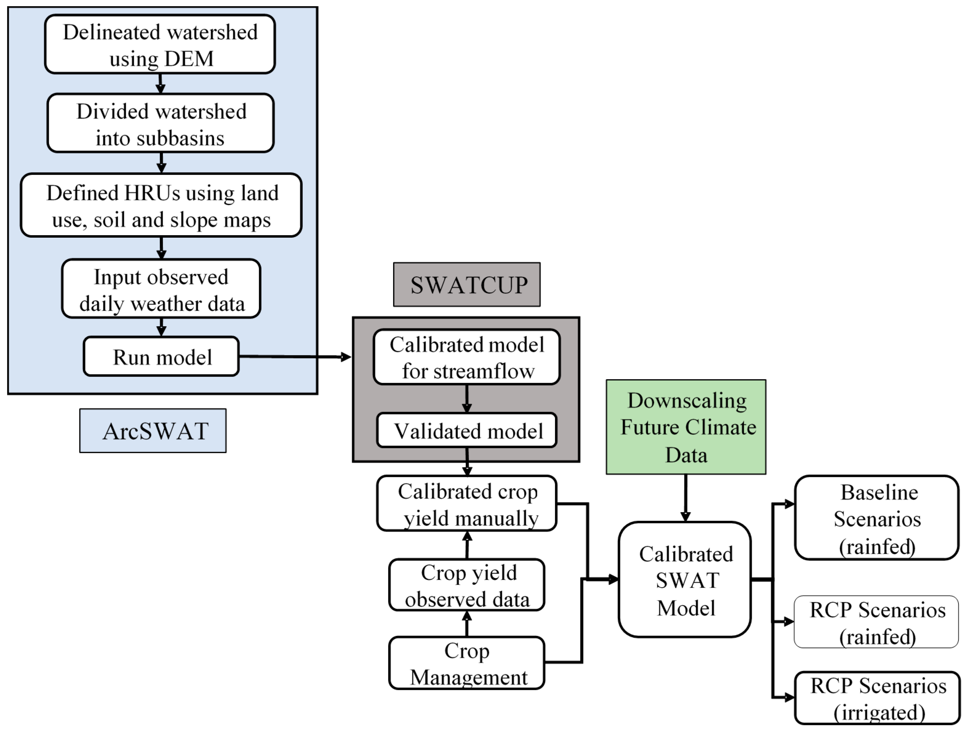
2.3. Model Setup, Calibration, and Validation

The watershed was discretized into 29 sub-basins using 3% flow accumulation area threshold, and all sub-basins were further discretized into hydrologic response units using 2, 5, and 5% thresholds for land use, soil, and slope classes, respectively. The Penman–Monteith method [38] was used to compute potential evapotranspiration. The modified soil conservation service (SCS) curve number method [27,31] and the Muskingum routing method [31] were used to estimate the surface runoff and the channel routing of the watershed.

A set of 17 parameters were selected for calibration representing surface, subsurface, and channel hydrologic responses (

Table 3. The list of parameters used for model calibration for the study watershed.

Parameter	Definition	Initial Range	Calibrated Value
Soil Water
SOL_K	Soil saturated hydraulic conductivity (mm/hr)	−25 to 25	7.15
SOL_AWC	Available soil water capacity (mm H2O/mm soil)	−25 to 25	19.15
Groundwater
ALPHA_BF	Baseflow recession constant (days)	0.01 to1	0.878
GW_DELAY	Groundwater delay (days)	1 to 500	32.50
GW_REVAP	Groundwater “revap” coefficient	0.01 to 0.2	0.087
REVAPMN	Re-evaporation threshold (mm H2O)	0.01 to 500	495.5
GWQMN	Threshold groundwater depth for return flow (mm H2O)	0.01 to 5000	3745
Surface Runoff
CN2	Curve number for moisture condition II	−0.3 to 0.3	0.064
EPCO	Plant uptake compensation factor	0.01 to 1	0.643
ESCO	Soil evaporation compensation factor	0.01 to 1	0.939
Channel Flow
CH_N(2)	Main channel Manning’s n	0.01 to 0.15	0.023
CH_K(2)	Main channel hydraulic conductivity (mm/hr)	5 to 500	491.5
Snow
SFTMP	Snowfall temperature (°C)	0 to 5	2.1
SMFMN	Melt factor for snow on December 21 (mm H2O/°C-day)	0 to 10	7.1
SMFMX	Melt factor for snow on June 21 (mm H2O/°C-day)	0 to 10	7.3
SMTMP	Snow melt base temperature (°C)	−2 to 5	3.1
TIMP	Snow pack temperature lag factor	0 to 1	0.35

). The parameters and their initial ranges were selected based on the suggestions from model developers presented in the SWAT 2012 manual [26] and a literature review of existing studies in areas with close proximity [39,40,41,42].

To represent the hydrological response of the watershed, hydrographs between observed and model-simulated monthly streamflow were compared at the watershed outlet (Figure 1). The model was calibrated for 15 years (1986–2000) with a 5-year warm-up period and was validated for another 15 years (2001–2015). For the calibration process, the Sequential Uncertainty Fitting version 2 (SUFI-2) algorithm [43] was applied, following the calibration protocol [28] and the technique described in Paul and Negahban-Azar [44]. Nash–Sutcliffe efficiency (NSE) was used as an objective function to measure the agreement between simulated and observed streamflow hydrographs. To evaluate the goodness of fit between the observation and the best simulation, three statistical criteria—correlation coefficient (R²), Nash–Sutcliffe coefficients (NSE), and percent bias (PBIAS)—were calculated. R² evaluates fit, NSE evaluates the peak flows, and PBIAS with low-magnitude values indicate accurate model simulation (positive and negative values indicate model overestimation and underestimation bias, respectively) [44]. According to [45], the streamflow for a monthly time-step has a satisfactory NSE greater than 0.50, a satisfactory R² greater than 0.60, and a satisfactory PBIAS should be ±15%. (

Table 4. Evaluation criteria for calibration and validation performance for the hydrologic model. Adapted from Moraisi et al. [44].

Measure	Very Good	Good	Satisfactory	Not Satisfactory
${\mathrm{R}}^2=\frac{{[{{\displaystyle \sum }}_{\mathrm{i}}\left({\mathrm{Y}}^{\mathrm{obs},\mathrm{i}}-{\mathrm{Y}}_{\mathrm{mean}}^{\mathrm{obs}}\right)\left({\mathrm{Y}}^{\mathrm{sim},\mathrm{i}}-{\mathrm{Y}}_{\mathrm{mean}}^{\mathrm{sim}}\right)]}^2}{{{\displaystyle \sum }}_{\mathrm{i}}\sqrt{{\left({\mathrm{Y}}^{\mathrm{obs},\mathrm{i}}-{\mathrm{Y}}_{\mathrm{mean}}^{\mathrm{obs}}\right)}^2}{{\displaystyle \sum }}_{\mathrm{i}}\sqrt{{\left({\mathrm{Y}}^{\mathrm{sim},\mathrm{i}}-{\mathrm{Y}}_{\mathrm{mean}}^{\mathrm{sim}}\right)}^2}}$	R2 > 0.85	0.0.75 < R2 ≤ 0.85	0.60 < R2 ≤ 0.75	R2 ≤ 0.6
$\mathrm{NSE}=1-\frac{{{\displaystyle \sum }}_{\mathrm{i}}{\left({\mathrm{Y}}^{\mathrm{obs}}-{\mathrm{Y}}^{\mathrm{sim}}\right)}^2}{{{\displaystyle \sum }}_{\mathrm{i}}{\left({\mathrm{Y}}^{\mathrm{obs}}-{\mathrm{Y}}_{\mathrm{mean}}^{\mathrm{obs}}\right)}^2}$	NSE > 0.80	0.70 < NSE ≤ 0.80	0.50 < NSE ≤ 0.70	NSE ≤ 0.50
$\mathrm{PBIAS}(\%)=\frac{{{\displaystyle \sum }}_{\mathrm{i}=1}^{\mathrm{n}}({\mathrm{Y}}^{\mathrm{obs}}-{\mathrm{Y}}^{\mathrm{sim}})}{{{\displaystyle \sum }}_{\mathrm{i}=1}^{\mathrm{n}}{\mathrm{Y}}^{\mathrm{obs}}}\times 100$	PBIAS < ±5	±5 ≤ PBIAS < ±10	±10 ≤ PBIAS < ±15	PBIAS ≥ ±15

R²: correlation coefficient, NSE: Nash–Sutcliffe coefficients, PBIAS: percent bias.

).

After obtaining the best estimates of the parameters for streamflow calibration, the model was calibrated and validated for annual crop yield for two major crops (corn and soybean) in the Monocacy River Watershed. Observed crop yields were collected for 1980–2015 from the USDA National Agricultural Statistics Service (USDA-NASS) [23]. Crop yields are reported by NASS at the county level in bushels/ac unit; however, the SWAT estimates in kg/ha (dry yield) with 20% moisture content at harvest time [46]. Since the Monocacy River Watershed lies within three counties, the average observed yield conversion from county level was averaged to watershed scale and presented here in kg/ha unit. For crop yield simulation, standard deviation (SD) and PBIAS were used as the evaluation criteria following methods used in previous studies [46,47].

2.4. Simulation Scenarios for Future Evaluation

After a successful calibration and validation process, the calibrated model was simulated for the combination of four GCMs, three RCPs, and two management approaches (

Table 5. Evaluation criteria for calibration and validation performance for the hydrologic model. Adapted from Moraisi et al. [45].

Categories	Model	Simulation Period	Climate Data
Baseline Scenario	Calibrated	1986–2000	NCDC Data
			CCSM4
			GFDL-ESM2M
			MIROC-ESM
			IPSL-CM5A-LR
With “Current Rainfed” and “Adaptive Irrigation” Management	RCPs 4.5/6.0/8.5	2025–2099	CCSM4
			GFDL-ESM2M
			MIROC-ESM
			IPSL-CM5A-LR

). The model configurations were designed in a logical way to evaluate the reasonable future impacts with respect to a current baseline condition. First, the SWAT model was calibrated for 15 years (1986–2000) and validated for another 15 years (2001–2015) using observed data from NCDC. Every GCM has their own historical climate data (1950–2000) from which each projection (RCPs 4.5–8.5) was estimated. The historical climate data were then used within the calibrated model as “reference data” for the baseline period (1986–2000) (Table 5). Three RCPs for the four GCMs were run with two sets of management conditions (24 scenarios in total, Table 5). To evaluate the climate change effects on watershed hydrology and crop yields results, all the scenarios were compared with the baseline period.

The simulation results were presented for two future time periods (2035–2049 and 2085–2099), representing mid- and late-century, respectively. All the results were compared to the baseline condition (1986–2000) to evaluate the impacts of climate change on irrigation demand. The relative changes in average monthly evapotranspiration, surface runoff, and water yield simulated from the SWAT model were evaluated under three RCPs and for both mid and late-century. The impact on future crop yields is also presented for both mid- and late-century for “current rainfed” and “adaptive irrigated” conditions. To analyze future impacts, all the results were shown as percent changes so that modeling uncertainties would not strongly affect the overall perspective.

To identify the potential hydrological components that influence crop yield, multiple machine learning techniques were evaluated, including decision tree and random forest. The decision tree approach was used in this study, as decision trees and/or their variants have been applied in water science and management sectors to predict the multitude of water-related predictor variables [48,49,50]. The decision tree is a non-parametric machine learning modeling method that splits the tree into branches based on the predictor variables according to the local optimal decision rule to predict the variable of interest [50]. The technique is more interpretable and fast to compute. Random forest is based on the fitting of an ensemble of uncorrelated decision trees to randomly subset the input data to get an optimum prediction by choosing the majority among the decision trees [50] but can be hard to interpret [48,49] and therefore was not used in this study.

3. Results and Discussion

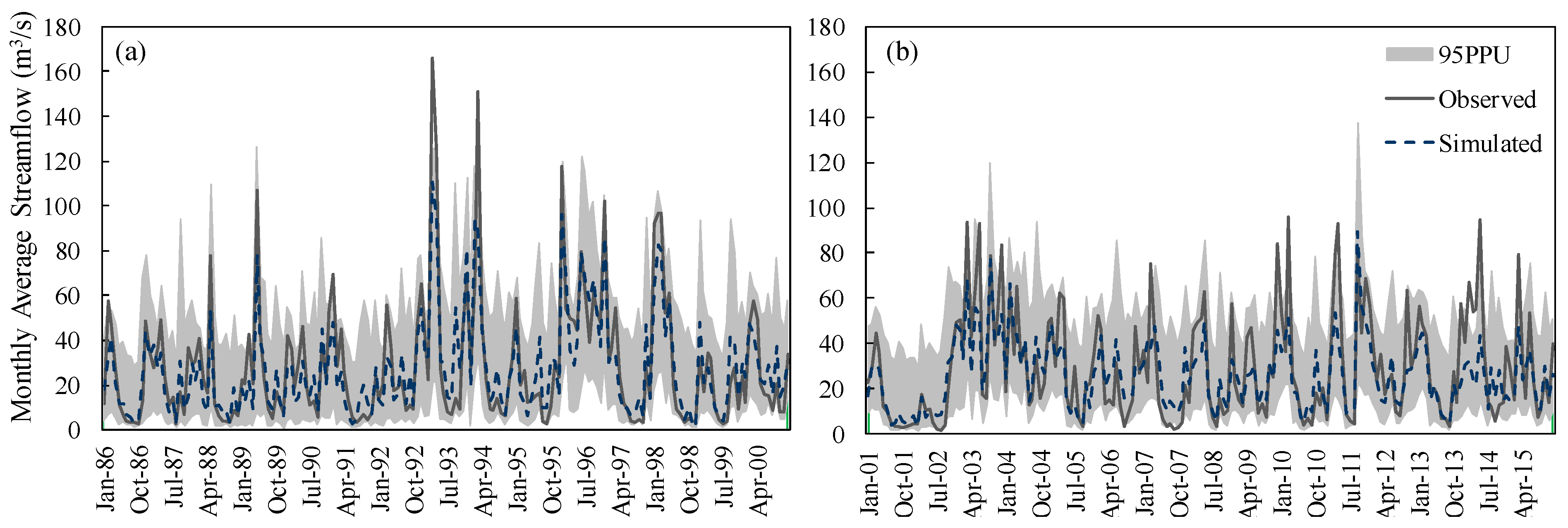
3.1. Evaluation of SWAT Performance

3.1.1. Model Performance for Hydrology

The observed monthly streamflow was captured well by the model simulation during both the calibration and the validation periods (Figure 3). The goodness of fit scores R², NSE, and PBIAS values were 0.78, 0.78, and 3.78 for calibration and 0.65, 0.65, and 5.8 for the validation period, respectively. According to the performance criteria suggested by [45], the calibration performance was “good”, and validation was “satisfactory” for predicting monthly streamflow in the Monocacy River Watershed (Table 4). From the hydrograph (Figure 3), it was noticeable that, during the validation period, the Monocacy River Watershed experienced drier periods than the calibration period, which resulted in comparatively low R² and NSE values for the validation period. After the successful model calibration, the calibrated parameters (Table 3) were inserted to the 28 models (Table 5) to simulate the streamflow under future climate projections.

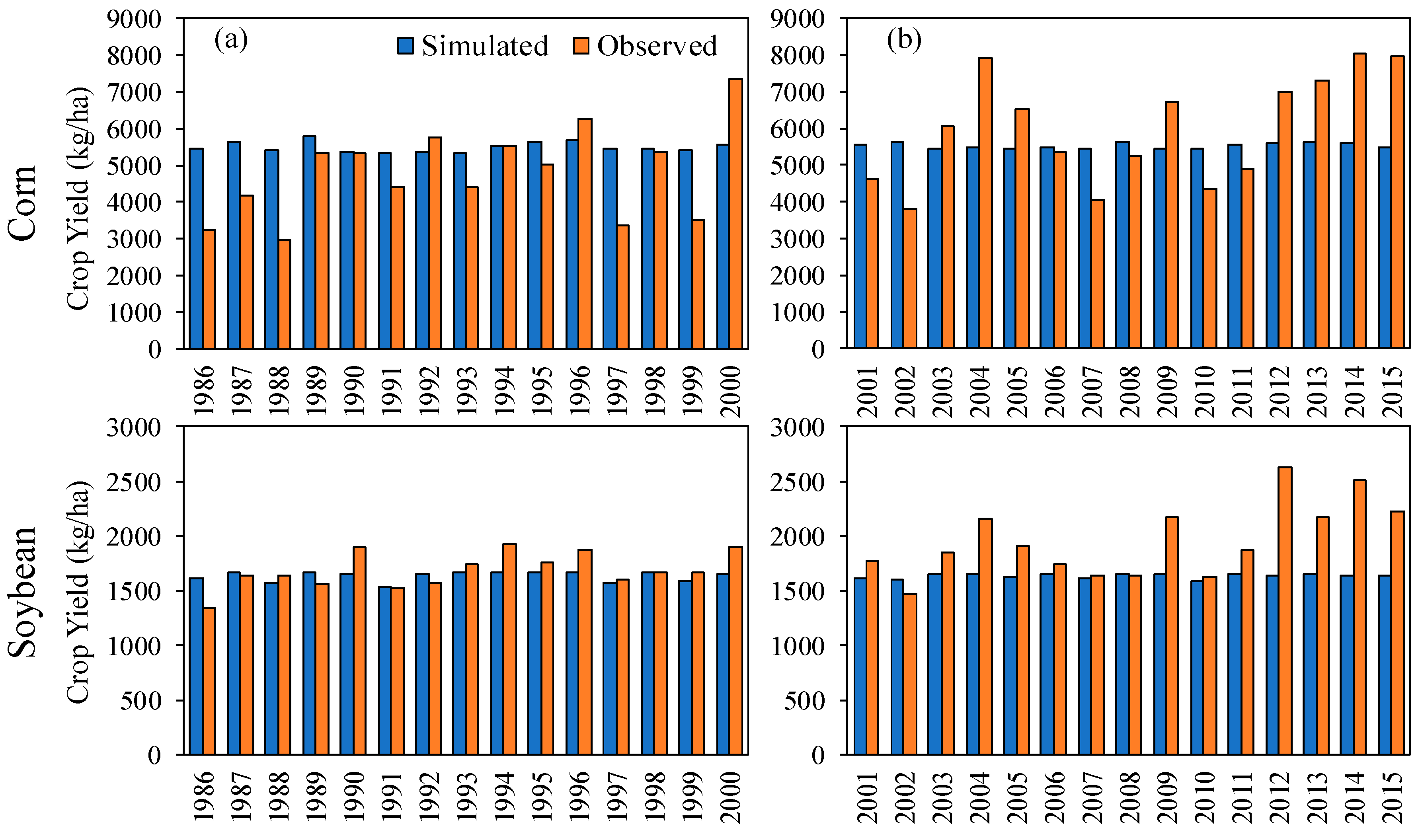
3.1.2. Model Performance for Crop Yield

The annual crop yields for corn and soybean were simulated and compared with the observed yields collected from USDA-NASS. The model was able to simulate the annual corn and soybean yields for both the calibration (1986–2000) and the validation (2001–2015) periods satisfactorily (Figure 4). The calibration and validation PBIAS values were −14.38% and 7.83% for corn yields and 3.21% and 15.58% for soybean yields, respectively.

The model’s prediction showed higher variations with wetter years and extremely dry years. The SD was estimated for simulated and observed corn and soybean yields in both the calibration and the validation periods to capture the interannual variability. During the calibration and the validation periods, the SD values for the observed corn yields were 1192.37 and 1421.18 kg/ha, respectively, which shows a larger difference than the observed soybean yields (157.1 and 329.15 kg/ha). Comparatively, the SWAT simulated crop yields showed less interannual variability for both corn and soybean yields. Smaller SD values were found for simulated corn yields, with 138.85 and 75.2 kg/ha during the calibration and the valuation periods, respectively. The lowest variability was obtained for the simulated soybean yields, with 43.35 and 20.9 kg/ha during calibration and valuation periods, respectively.

In this study, the model was designed for rainfed corn and soybean. Although the watershed is dominated by non-irrigated (rainfed) management system, minimal irrigation is applied based on the field requirements (soil condition, crop requirement). In addition, due to lack of field data, we used a fixed amount of fertilizer application throughout the simulation period. Therefore, irrigation application during seasonal droughts and different amount of fertilization application were not considered during the model development.

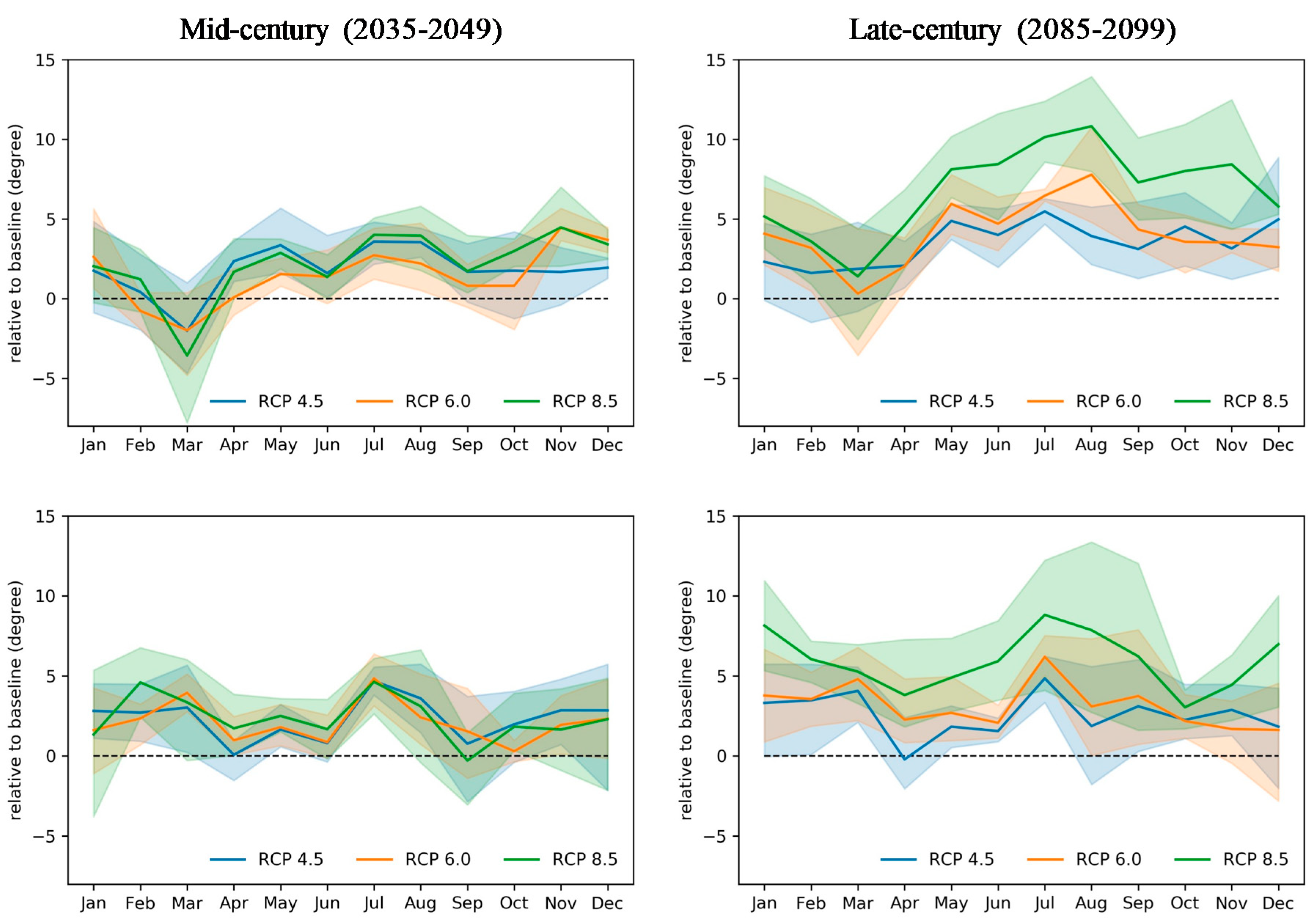
3.2. Future Climate Projections

The projected climate changes were analyzed for two distinct periods (2035–2049 and 2085–2099) across all four GCMs and three RCPs and compared to the baseline condition (1986–2000). Figure 5 shows the relative percentage changes of average monthly precipitation for 2035–2049 and 2085–2099 under the three RCP scenarios. Figure 6 shows the relative change in the monthly maximum and minimum temperatures for three RCPs compared to the baseline period. It was noticeable that, compared to baseline period, the average monthly precipitation and maximum and minimum temperatures were varied among all three RCPs, with a higher uncertainty for late-century compared to mid-century.

During mid-century, the monthly precipitation increased largely from December to March and from June to August, ranging from 9 to 35% and 6 to 36% increases, respectively, across all RCPs (Figure 5). Similarly, during late-century, the monthly precipitation increased largely during November to March and June to August, ranging from 15–48% across all RCPs, except in June for RCP 6, when the mean precipitation decreased (−3%). However, monthly precipitation was projected to decrease in October for all RCPs in both mid (−15 to −26%) and late-century (−1 to −7%). Larger uncertainties for the monthly precipitation were found during January and March during mid-century and February and March during late-century. However, the largest anomaly in precipitation was found for RCP 6 during mid-century.

Predictions by the ensemble of four GCMs showed the highest monthly temperature change during the summer months of June, July, and August. From Figure 6, it was noticeable that both maximum and minimum temperatures during late-century (2085–2099) would be much higher than mid-century (2035–2049). The largest monthly maximum (10.7 °C) and minimum temperature (8.8 °C) changes were found during the 2085–2099 period under the RCP 8.5 scenario. The magnitude of the projected maximum temperature varies widely during the late-century. These combined effects of precipitation and temperature changes indicate that wetter fall and spring and a drier late summer (harvest period) can be anticipated in the future.

3.3. Impact of Future Climate Projections

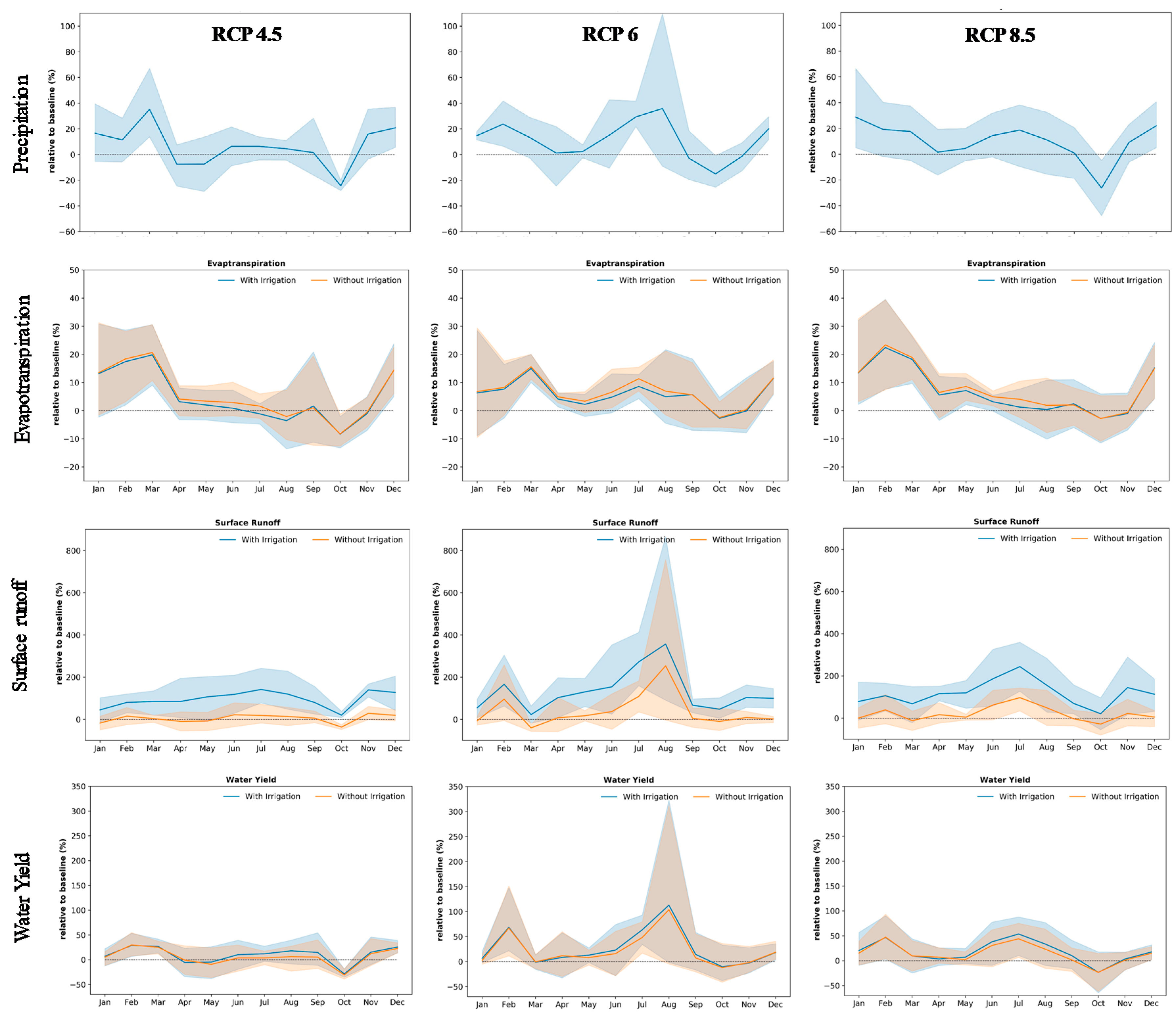
3.3.1. Impact on Water Balance

A water balance provides crucial information about the hydrological characteristics of the watershed [51]. The changes in water balance in response to climate change can have a profound impact on agricultural productivity and irrigation requirements [47]. Since seasonal variability influences the crop productivity and yield, monthly water balance components were analyzed to understand the changes at the seasonal scale. The comparison of water balance components between two management scenarios (rainfed and irrigated conditions) are shown in Figure 7 and Figure 8. The SWAT simulated outcomes showed that the differences among the GCM projections led to differences in water balance across all emission scenarios and between the management scenarios.

In response to increased precipitation and temperature (Figure 3 and Figure 4), there was an overall increase in the average monthly surface runoff and water yield for both mid and late-century (Figure 7 and Figure 8). Water yield is defined as total amount of blue water that is leaving the HRU and entering into the main channel and was estimated as the sum of surface runoff, lateral flow, and base flow. Average monthly surface runoff showed increases up to 21, 254, and 97% for mid-century and increases up to 98, 82, and 163% for late-century under RCPs 4.5, 6, and 8.5, respectively. Similar results were found for water yield where, on average, water yield increased under all three RCPs. According to all four GCMs, the water yield increase at the largest scale under RCP 6 was up to 103.86% for mid-century (Figure 7) and up to 83% under RCP 8.5 for late-century (Figure 8) compared to the baseline condition. During mid-century, higher precipitation under RCP 6 contributed to higher surface runoff, which resulted in higher water yields compared to other RCPs (Figure 7). The average monthly evapotranspiration showed comparatively smaller increments up to 21, 16, and 23% for mid-century and 26, 34, and 57% for late-century under RCPs 4.5, 6, and 8.5.

Under irrigated conditions, it was noticeable that potential temperature and precipitation change resulted in higher plant stress, with irrigation needed to mitigate this plant stress. This indicates that higher temperatures may induce more evaporative loss that elevates water stress and thus increases the demand for irrigation. The irrigated condition model simulations showed that corn production had mean annual irrigation needs of 127–146 m³/ha and 131–137 m³/ha for mid-century and late-century, respectively. The mean annual irrigation needs for soybeans production were projected to be 131–155 m³/ha and 147–161 m³/ha during mid-century and late-century, respectively.

As a result of additional irrigation application, average monthly surface runoff increased, especially between June to September (Figure 7 and Figure 8). Higher surface runoff resulted in higher water yield during mid- and late-centuries across all emission scenarios compared to the rainfed condition (Figure 7 and Figure 8). Compared to baseline condition, the corresponding water yield increased up to 113% and 100% during mid-century and late-century, respectively.

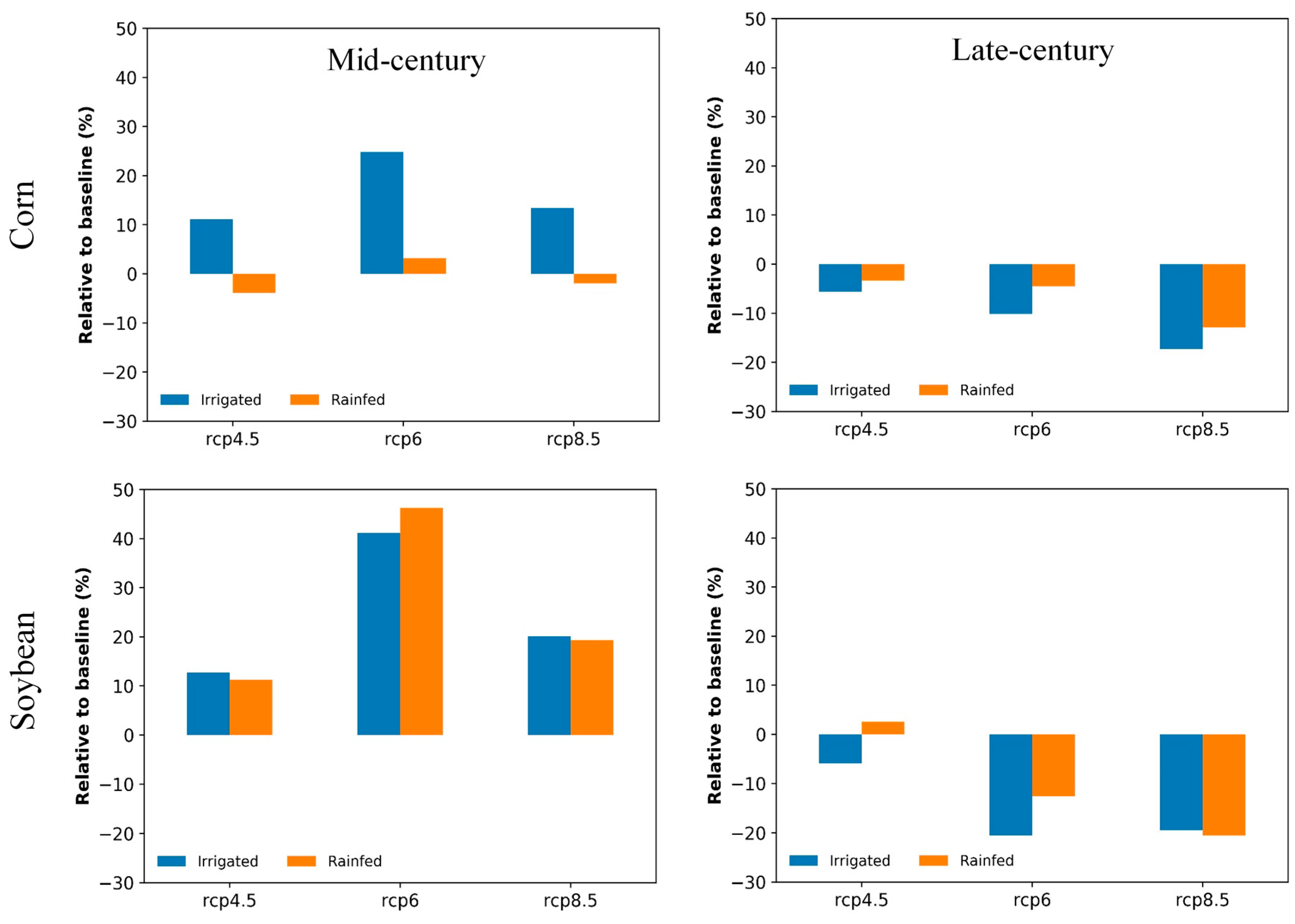
3.3.2. Impact on Crop Yield

The simulated results suggest that, under the “current rainfed” condition, future climate changes might contribute to a wide variation in corn and soybean yields (Figure 9). During the mid-century, a small increase in mean annual corn yields was found under RCP 6 (+3.2%) with slight declines under RCP 4.5 (−3.8%) and 8.5 (−1.9%) scenarios relative to the baseline period. Unlike the corn yield, the mean soybean yield increased during mid-century by 11.2%, 46.3%, and 19.3% under RCP 4.5, RCP 6, and RCP 8.5, respectively.

Both corn and soybean yields decreased across all RCPs in the late-century, except in RCP 4.5, where soybean yields slightly increased. For corn, the mean annual yield declined by 3.4, 4.5, and 13% under RCP 4.5, RCP 6, and RCP 8.5, respectively. Meanwhile, the mean annual soybean yield decreased by 12.6 and 20.5% under RCP 6 and RCP 8.5, respectively, and increased by 2.6% under the RCP 4.5 scenario.

These results indicate that the higher temperatures during April to May may result in overall decline in corn yields during mid- and late-century and soybean yields during late-century. However, during mid-century, the combined effect of precipitation and temperature change might lead to a positive impact on soybean production in this region. Overall, the aggregate impact of four GCMs shows that the relative decline in yield for both corn and soybeans was larger for RCP 6 and 8.5 in the late-century. The less water availability during the crop growing period due to higher temperatures may result in a substantial decline in corn and soybean production in the late-century. A previous study showed that dry conditions in the corn planting period are crucial for seed germination and higher yield [52]. A study by Kukal and Irmak [9] also found that temperature increases have negative impacts on soybean yields in the US Great Plains.

The frequency and the intensity of irrigation can significantly influence plant growth and watershed hydrology [53]. Irrigation application did not show any clear improvement in crop growth in this case study compared to the rainfed condition, except for increased corn yield during mid-century as a result of irrigation. Under adaptive irrigated conditions, the mean corn yield increased by 11, 25, and 13% for RCPs 4.5, 6, and 8.5, respectively, in mid-century. Some crops, such as corn, are highly sensitive to plant water stress [54], thus, additional irrigation during critical stages of maturity results in higher yield [55]. As a result of supplementary water through irrigation during water stress, the corn yield improved compared to the rainfed condition. However, during late-century, under irrigated condition, corn yields declined up to 17% compared to the rainfed condition (Figure 9, Late-century).

In the case of soybeans, the effect of irrigation on mean soybean yields varied across climate scenarios and time periods. In mid-century, irrigation marginally improved the soybean yield by 1.4% and 1% under RCPs 4.5 and 8.5, respectively, compared to rainfed condition, while a 5% decline was found under RCP 6. During the late-century, the mean soybean yields declined up to 20.5% compared to baseline conditions.

Increased surface runoff due to additional irrigation practices has the potential to increase nutrient transport to surface waters. A study by Sun et. al. [56] found that continuous irrigation without soil conservation practices could reduce soil quality and crop production. The decline in both corn and soybean yield during late-century could be due to the effect of prolonged irrigation on soil properties (i.e., nutrient content). This suggests that watershed management efforts should focus on developing other adaptation strategies, including irrigation timing and frequency, with fertilization application based on soil characteristics to address the effects of climate change on sustainable agricultural production.

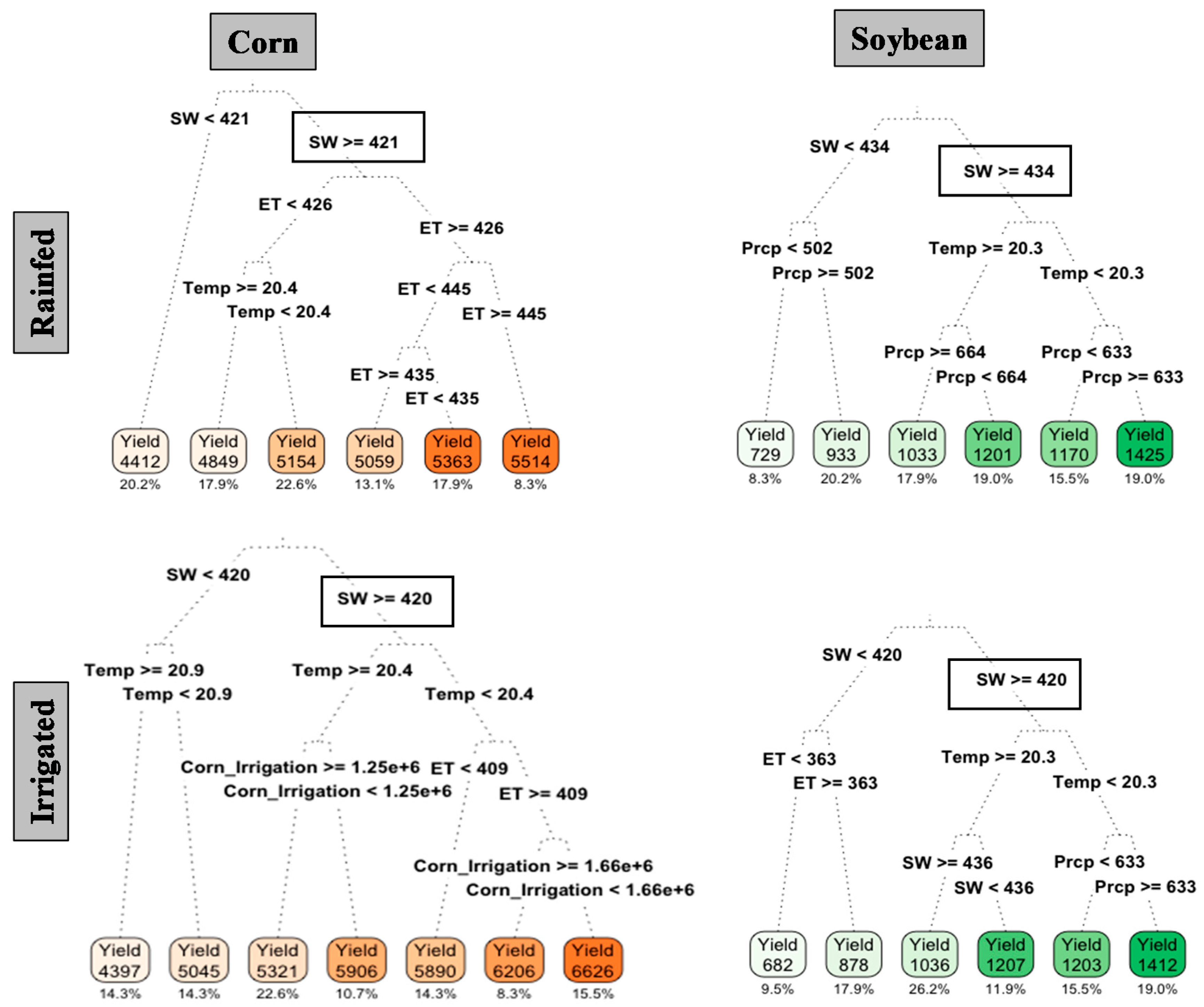
3.4. Selecting Important Predictors for Adaptation

The future projections of corn and soybean yields based on the three RCP scenarios were further interpreted with the decision trees to provide clear guidance to decision makers. Within the decision trees, variables were partitioned based on a set of rules embedded in a decision tree, where each node splits according to a decision rule. The algorithm selects the best feature among the randomly selected attributes (e.g., precipitation, temperature, soil moisture) to predict the optimum crop yield under these conditions. Figure 10 shows the decision tree results for corn and soybean yields for both irrigated and rainfed conditions under RCP 4.5. Each decision tree was based on precipitation, soil water storage, evapotranspiration, temperature, and irrigation requirement (during irrigated condition) as predictor variables. The regression tree was applied for each RCP that resulted in the most simulated values in the terminal nodes (i.e., crop yield).

The constructed decision trees showed that, for RCP 4.5, the first split was always based on soil water storage (Figure 10). For both management practices, the right node (interested boxes) was used as a decisive split for corn (SW ≥ 421 and 420) and soybean (SW ≥ 434 and 420) yields. Moving down the right nodes (inserted boxes), the larger portions of the crop yields (i.e., corn and soybeans) were found in all decision trees. The right nodes represent the largest percentage of the total crop yields, and thus were used as decisive splits. For example, under RCP 4.5, the corresponding percentages of these right nodes were sums of 79.8, 71.5, 71.4, and 72.6%.

Unlike RCP 4.5, temperature was found as the most important variable for RCPs 6 and 8.5, which was placed in the right node after the first split under both runs (rainfed and irrigated) (Supplementary Figure S1). However, for corn yields under RCP 6 and rainfed condition, precipitation was found as the most important variable.

It is also notable that, with irrigation application, a slight mitigation (i.e., higher yield) may be achieved for corn production (Figure 10). For example, a similar split (SW > 420) in the right node showed irrigation application could have resulted higher corn production (5188–6844 kg/ha) compared to rainfed (5081–5514 kg/ha). Under all RCPs, “crop irrigation” variable was used to split the node where higher irrigation application showed higher corn yield compared to rainfed condition (Figure 10). Similar results were found by Vogel et al.’s [57] analysis of a global crop yield dataset, where temperature-related extremes showed a stronger association with maize, soybeans, rice, and spring wheat yield anomalies, and irrigation partly mitigated negative effects of these extremes.

4. Conclusions

This study evaluated future climate change impacts on hydrology and crop yields in Monocacy River Watershed as a representative agricultural watershed in the Mid-Atlantic. Downscaled and bias corrected climate projections from four GCMs and three RCP scenarios were used as climate inputs to the SWAT model. The SWAT model was successfully applied to capture the hydrologic conditions of the watershed and simulate future climate change impacts on annual crop yields. The hydrologic components (water yield, evapotranspiration, and surface runoff) and crop yields (corn and soybean) were assessed for mid-century (2035–2049) and late-century (2085–2099) periods.

Results indicated that crop yields in this watershed will be affected by projected climate change, subject to the uncertainty of the modeling results. Precipitation increases in the watershed resulted in greater surface runoff, although evapotranspiration changes were minimal. Under the current rainfed condition, corn yield is expected to decline in both mid- and late-centuries across all RCP scenarios. Whereas, soybean yield is predicted to increase for mid-century but decline by late-century. To examine the impact of irrigation as an adaptive measure for future climate change scenarios, irrigation practices were applied to the model and compared with current rainfed management practices. The results suggest that irrigation may be helpful in improving corn yield during mid-century across all scenarios, however, prolonged irrigation has a negative impact on both corn and soybean yields compared to rainfed conditions possibly due to soil nutrient depletion following extended periods of irrigation.

The crop yields were analyzed further using a decision tree algorithm. The results indicated that corn and soybean yields were mainly influenced by soil moisture, temperature, and precipitation as well as by management practices (i.e., rainfed or irrigated). The outcomes from this study can be used as a guideline for water resource managers to plan the required adaptive management strategies to maintain expected corn and soybean yields in the coming century.

References

1. Vaghefi, S.A.; Abbaspour, K.C.; Faramarzi, M.; Srinivasan, R.; Arnold, J.G. Modeling Crop Water Productivity Using a Coupled SWAT–MODSIM Model. Water 2017, 9, 157. [Google Scholar] [CrossRef] [Green Version]
2. Pathak, T.B.; Maskey, M.L.; Dahlberg, J.A.; Kearns, F.; Bali, K.M.; Zaccaria, D. Climate Change Trends and Impacts on California Agriculture: A Detailed Review. Agronomy 2018, 8, 25. [Google Scholar] [CrossRef] [Green Version]
3. Paul, M.; Rajib, M.A.; Ahiablame, L. Spatial and Temporal Evaluation of Hydrological Response to Climate and Land Use Change in Three South Dakota Watersheds. J. Am. Water Resour. Assoc. 2017, 53, 69–88. [Google Scholar] [CrossRef]
4. Rajib, A.; Ahiablame, L.; Paul, M. Modeling the effects of future land use change on water quality under multiple scenarios: A case study of low-input agriculture with hay/pasture production. Sustain. Water Qual. Ecol. 2016, 8, 50–66. [Google Scholar] [CrossRef] [Green Version]
5. USGCRP. Impacts, Risks, and Adaptation in the United States: Fourth National Climate Assessment; Reidmiller, D.R., Avery, C.W., Easterling, D.R., Kunkel, K.E., Lewis, K.L.M., Maycock, T.K., Stewart, B.C., Eds.; U.S. Global Change Research Program: Washington, DC, USA, 2018. [Google Scholar]
6. Vaghefi, S.A.; Mousavi, S.J.; Abbaspour, K.C.; Srinivasan, R.; Yang, H. Analyses of the impact of climate change on water resources components, drought and wheat yield in semiarid regions: Karkheh River Basin in Iran. Hydrol. Process. 2014, 28, 2018–2032. [Google Scholar] [CrossRef]
7. Paul, M. Impacts of Land Use and Climate Changes on Hydrological Processes in South Dakota Watersheds. Master’s Thesis, South Dakota State University, Brookings, SD, USA, 2016. [Google Scholar]
8. Ahiablame, L.; Sinha, T.; Paul, M.; Ji, J.-H.; Rajib, A. Streamflow response to potential land use and climate changes in the James River watershed, Upper Midwest United States. J. Hydrol. Reg. Stud. 2017, 14, 150–166. [Google Scholar] [CrossRef]
9. Kukal, M.S.; Irmak, S. Climate-Driven Crop Yield and Yield Variability and Climate Change Impacts on the U.S. Great Plains Agricultural Production. Sci. Rep. 2018, 8, 1–18. [Google Scholar] [CrossRef] [Green Version]
10. Mourtzinis, S.; Specht, J.E.; Lindsey, L.E.; Wiebold, W.J.; Ross, J.; Nafziger, E.D.; Kandel, H.J.; Mueller, N.; DeVillez, P.L.; Arriaga, F.J.; et al. Climate-induced reduction in US-wide soybean yields underpinned by region- and in-season-specific responses. Nat. Plants 2015, 1, 14026. [Google Scholar] [CrossRef]
11. Smith, W.; Grant, B.; Desjardins, R.; Kroebel, R.; Li, C.; Qian, B.; Worth, D.; McConkey, B.; Drury, C. Assessing the effects of climate change on crop production and GHG emissions in Canada. Agric. Ecosyst. Environ. 2013, 179, 139–150. [Google Scholar] [CrossRef]
12. Goldblum, D. Sensitivity of Corn and Soybean Yield in Illinois to Air Temperature and Precipitation: The Potential Impact of Future Climate Change. Phys. Geogr. 2009, 30, 27–42. [Google Scholar] [CrossRef]
13. Ozturk, I.; Sharif, B.; Baby, S.; Jabloun, M.; Olesen, J.E. The long-term effect of climate change on productivity of winter wheat in Denmark: A scenario analysis using three crop models. J. Agric. Sci. 2017, 155, 733–750. [Google Scholar] [CrossRef]
14. Chesapeake Bay Foundation. Climate Change and the Chesapeake Bay: Challenges, Impacts, and the Multiple Benefits of Agricultural Conservation Work; Reports; Chesapeake Bay Foundation: Annapolis, MD, USA, 2007; Available online: https://umaryland.on.worldcat.org/search?queryString=no%3A+192021227#/oclc/192021227 (accessed on 30 October 2019).
15. Hayhoe, K.; Wake, C.P.; Huntington, T.G.; Luo, L.; Schwartz, M.D.; Sheffield, J.; Wood, E.; Anderson, B.; Bradbury, J.; DeGaetano, A.; et al. Past and future changes in climate and hydrological indicators in the US Northeast. Clim. Dyn. 2007, 28, 381–407. [Google Scholar] [CrossRef]
16. Luck, M.; Landis, M.; Gassert, F. Aqueduct Water Stress Projections: Decadal Projections of Water Supply and Demand Using CMIP5 GCMs; Techical Note; World Resources Institute: Washington, DC, USA, 2015. [Google Scholar]
17. Altieri, M.A.; Nicholls, C.I.; Henao, A.; Lana, M.A. Agroecology and the design of climate change-resilient farming systems. Agron. Sustain. Dev. 2015, 35, 869–890. [Google Scholar] [CrossRef] [Green Version]
18. Uniyal, B.; Dietrich, J.; Vu, N.Q.; Jha, M.K.; Arumí, R.J.L. Simulation of regional irrigation requirement with SWAT in different agro-climatic zones driven by observed climate and two reanalysis datasets. Sci. Total Environ. 2019, 649, 846–865. [Google Scholar] [CrossRef]
19. Gharibdousti, S.R.; Kharel, G.; Miller, R.B.; Linde, E.; Stoecker, A. Projected Climate Could Increase Water Yield and Cotton Yield but Decrease Winter Wheat and Sorghum Yield in an Agricultural Watershed in Oklahoma. Water 2019, 11, 105. [Google Scholar] [CrossRef] [Green Version]
20. Thomas, A. Agricultural irrigation demand under present and future climate scenarios in China. Glob. Planet. Chang. 2008, 60, 306–326. [Google Scholar] [CrossRef]
21. Moriondo, M.; Bindi, M.; Kundzewicz, Z.W.; Szwed, M.; Choryński, A.; Matczak, P.; Radziejewski, M.; McEvoy, D.; Wreford, A. Impact and adaptation opportunities for European agriculture in response to climatic change and variability. Mitig. Adapt. Strat. Glob. Chang. 2010, 15, 657–679. [Google Scholar] [CrossRef]
22. Stricevic, R.; Cosic, M.; Djurovic, N.; Pejic, B.; Maksimovic, L. Assessment of the FAO AquaCrop model in the simulation of rainfed and supplementally irrigated maize, sugar beet and sunflower. Agric. Water Manag. 2011, 98, 1615–1621. [Google Scholar] [CrossRef]
23. USDA-NASS. Cropland Data Layer. Available online: https://www.nass.usda.gov/Research_and_Science/ (accessed on 15 June 2019).
24. Upper Monocacy River Watershed Characterization Plan Prepared by Carroll County Bureau of Resource Management. Available online: https://www.carrollcountymd.gov/media/10356/upper-monocacy-river-characterization-plan.pdf (accessed on 15 March 2019).
25. Schultz, C.; Palmer, J. Seasonal Steady-State Ground Water/Stream Flow Model of the Upper Monocacy River Basin; ICPRB: Rockville, MD, USA, 2008; p. 46. [Google Scholar]
26. Arnold, J.G.; Moriasi, D.N.; Gassman, P.W.; Abbaspour, K.C.; White, M.J.; Srinivasan, R.; Santhi, C.; Harmel, R.; Van Griensven, A.; Van Liew, M.W. SWAT: Model use, calibration, and validation. Trans. ASABE 2012, 55, 1491–1508. [Google Scholar] [CrossRef]
27. Arnold, J.G.; Srinivasan, R.; Muttiah, R.S.; Williams, J.R. Large area hydrologic modeling and assessment part I: Model development. J. Am. Water Resour. Assoc. 1998, 34, 73–89. [Google Scholar] [CrossRef]
28. Abbaspour, K.C.; Rouholahnejad, E.; Vaghefi, S.; Srinivasan, R.; Yang, H.; Kløve, B. A continental-scale hydrology and water quality model for Europe: Calibration and uncertainty of a high-resolution large-scale SWAT model. J. Hydrol. 2015, 524, 733–752. [Google Scholar] [CrossRef] [Green Version]
29. Baker, T.J.; Miller, S. Using the Soil and Water Assessment Tool (SWAT) to assess land use impact on water resources in an East African watershed. J. Hydrol. 2013, 486, 100–111. [Google Scholar] [CrossRef]
30. Ahmadzadeh, H.; Morid, S.; Delavar, M.; Srinivasan, R. Using the SWAT model to assess the impacts of changing irrigation from surface to pressurized systems on water productivity and water saving in the Zarrineh Rud catchment. Agric. Water Manag. 2016, 175, 15–28. [Google Scholar] [CrossRef]
31. Neitsch, S.L.; Arnold, J.G.; Kiniry, J.R.; Williams, J.R. Soil and Water Assessment Tool Theoretical Documentation Version 2009; Texas Water Resources Institute: Tamu, TX, USA, 2011. [Google Scholar]
32. Winchell, M.; Srinivasan, R.; Diluzio, M.; Arnold, J. Arcswat Interface for Swat 2012: User Guider; Blackland Research Center: Temple, TX, USA, 2013. [Google Scholar]
33. US Department of Interior. National Elevation Dataset; US Department of Interior: Washington, DC, USA, 2006.
34. Tan, M.L.; Ibrahim, A.L.; Yusop, Z.; Chua, V.P.; Chan, N.W. Climate change impacts under CMIP5 RCP scenarios on water resources of the Kelantan River Basin, Malaysia. Atmos. Res. 2017, 189, 1–10. [Google Scholar] [CrossRef]
35. Reclamation, U. Downscaled CMIP3 and CMIP5 Climate and Hydrology Projections: Release of Hydrology Projections, Comparison with Preceding Information, and Summary of User Needs; Bureau of Reclamation, Technical Services Center: Denver, CO, USA, 2014. [Google Scholar]
36. Change, I.C. Mitigation of Climate Change; IPCC: Geneva, Switzerland, 2014; p. 1454. [Google Scholar]
37. Allen, R.G.; Pereira, L.S.; Raes, D.; Smith, M. FAO Irrigation and Drainage Paper No. 56; FAO: Rome, Italy, 1998; p. 156. [Google Scholar]
38. Sibbons, J.L.H.; Monteith, J.L.; Penman, H.L.; Priestle, C. The horizontal transport of heat and moisture—A micrometeorological study. Q. J. R. Meteorol. Soc. 1965, 91, 236. [Google Scholar]
39. Chu, T.; Shirmohammadi, A.; Montas, H.; Abbott, L.; Sadeghi, A. Watershed Level BMP Evaluation with SWAT Model. In Proceedings of the 2005 ASAE Annual Meeting, Tampa, FL, USA, 17–20 July 2005. [Google Scholar]
40. Sadeghi, A.M.; Yoon, K.; Graff, C.; Mccarty, G.; McConnell, L.; Shirmohammadi, A.; Hively, D.; Sefton, K. Assessing the Performance of SWAT and AnnAGNPS Models in a Coastal Plain Watershed, Choptank River, Maryland, U.S.A. In Proceedings of the 2007 ASAE Annual Meeting, Minneapolis, MN, USA, 17–20 June 2007. [Google Scholar]
41. Sexton, A.M.; Shirmohammadi, A.; Sadeghi, A.M.; Montas, H.J. Impact of Parameter Uncertainty on Critical SWAT Output Simulations. Trans. ASABE 2011, 54, 461–471. [Google Scholar] [CrossRef]
42. Sexton, A.M.; Sadeghi, A.M.; Zhang, X.; Srinivasan, R.; Shirmohammadi, A. Using NEXRAD and Rain Gauge Precipitation Data for Hydrologic Calibration of SWAT in a Northeastern Watershed. Trans. ASABE 2010, 53, 1501–1510. [Google Scholar] [CrossRef]
43. Abbaspour, K.C. SWAT Calibration and Uncertainty Program—A User Manual; Swiss Federal Institute of Aquatic Science and Technology: Eawag, Switzerland, 2013. [Google Scholar]
44. Paul, M.; Negahban-Azar, M. Sensitivity and uncertainty analysis for streamflow prediction using multiple optimization algorithms and objective functions: San Joaquin Watershed, California. Model. Earth Syst. Environ. 2018, 4, 1509–1525. [Google Scholar] [CrossRef]
45. Moriasi, D.N.; Gitau, M.W.; Pai, N.; Daggupati, P. Hydrologic and Water Quality Models: Performance Measures and Evaluation Criteria. Trans. ASABE 2015, 58, 1763–1785. [Google Scholar] [CrossRef] [Green Version]
46. Srinivasan, R.; Zhang, X.; Arnold, J.G. SWAT Ungauged: Hydrological Budget and Crop Yield Predictions in the Upper Mississippi River Basin. Trans. ASABE 2010, 53, 1533–1546. [Google Scholar] [CrossRef]
47. Woznicki, S.A.; Nejadhashemi, A.P.; Parsinejad, M. Climate change and irrigation demand: Uncertainty and adaptation. J. Hydrol. Reg. Stud. 2015, 3, 247–264. [Google Scholar] [CrossRef]
48. Tyralis, H.; Papacharalampous, G.A.; Langousis, A. A Brief Review of Random Forests for Water Scientists and Practitioners and Their Recent History in Water Resources. Water 2019, 11, 910. [Google Scholar] [CrossRef] [Green Version]
49. Iorgulescu, I.; Beven, K.J. Nonparametric direct mapping of rainfall-runoff relationships: An alternative approach to data analysis and modeling? Water Resour. Res. 2004, 40, W08403. [Google Scholar] [CrossRef] [Green Version]
50. Breiman, L.; Friedman, J.H.; Olshen, R.A.; Stone, C.J. Classification and Regression Trees; CRC Press: Boca Raton, FL, USA, 1984. [Google Scholar]
51. Flerchinger, G.N.; Cooley, K. A ten-year water balance of a mountainous semi-arid watershed. J. Hydrol. 2000, 237, 86–99. [Google Scholar] [CrossRef]
52. Hu, Q.; Buyanovsky, G. Climate Effects on Corn Yield in Missouri. J. Appl. Meteorol. 2003, 42, 1626–1635. [Google Scholar] [CrossRef]
53. Xie, X.; Cui, Y. Development and test of SWAT for modeling hydrological processes in irrigation districts with paddy rice. J. Hydrol. 2011, 396, 61–71. [Google Scholar] [CrossRef]
54. Mustek, J.T.; Dusek, D.A. Irrigated Corn Yield Response to Water. Trans. ASAE 1980, 23, 0092–0098. [Google Scholar] [CrossRef] [Green Version]
55. Lewis, J. Estimating Irrigation Water Requirements to Optimize Crop Growth (FS-447); University of Maryland Extension: Cumberland, MD, USA, 2014. [Google Scholar]
56. Sun, H.; Zhang, X.; Liu, X.; Ju, Z.; Shao, L. The long-term impact of irrigation on selected soil properties and grain production. J. Soil Water Conserv. 2018, 73, 310–320. [Google Scholar] [CrossRef]
57. Vogel, E.; Donat, M.G.; Alexander, L.V.; Meinshausen, M.; Ray, D.K.; Karoly, D.; Meinshausen, N.; Frieler, K. The effects of climate extremes on global agricultural yields. Environ. Res. Lett. 2019, 14, 054010. [Google Scholar] [CrossRef]
Figure 1. Generated map of the Monocacy River Watershed with selected weather stations and the US Geological Survey streamflow gauge stations at respective watershed outlets.
Climate 08 00139 g001
Figure 2. Comprehensive approach of future climate model application in the Soil and Water Assessment Tool (SWAT) model. ArcGIS-ArcView extension and interface for SWAT (ArcSWAT) and Calibration Uncertainty Program for SWAT (SWATCUP) were used for model setup and model calibration, respectively, showing the digital elevation model (DEM), the hydrologic response units (HRU), and the representative concentration pathway (RCP).
Climate 08 00139 g002
Figure 3. Hydrographs showing the comparison of observed and simulated average monthly streamflow during (a) calibration (1986–2000) and (b) validation (2001–2015) period at the outlet of the Monocacy River Watershed.
Climate 08 00139 g003
Figure 4. Comparison of National Agricultural Statistics Service (NASS)-observed and SWAT-simulated crop yields for corn and soybean for the (a) calibration (1986–2000) and the (b) validation period (2001–2015).
Climate 08 00139 g004
Figure 5. Seasonal variation of monthly precipitation during mid (2035–2049) and late century (2085–2099) relative to baseline period (1986–2000) for three RCPs (4.5, 6, and 8.5). The straight lines show the mean monthly precipitation, and the shaded area shows the range of the precipitation variation within the global climate models (GCMs).
Climate 08 00139 g005
Figure 6. Seasonal variation of monthly maximum and minimum temperatures during mid (2035–2049) and late century (2085–2099) relative to baseline period (1986–2000) for three RCPs (4.5, 6, and 8.5). The straight lines show the mean monthly maximum and minimum temperatures, and the shaded area shows the range of the temperature variation within the GCMs.
Climate 08 00139 g006
Figure 7. Changes in monthly precipitation, evapotranspiration, surface runoff, and water yield for mid-century (2035–2049) under three scenarios: RCP 4.5, RCP 6, and RCP 8.5. The results are presented as relative the percentage change compared to the baseline period (1986–2000).
Climate 08 00139 g007
Figure 8. Changes in monthly precipitation, evapotranspiration, surface runoff, and water yield for late-century (2085–2099) under three scenarios: RCP 4.5, RCP 6, and RCP 8.5. The results are presented as the relative percentage change compared to the baseline period (1986–2000).
Climate 08 00139 g008
Figure 9. Relative change in crop yield for corn and soybean under three RCPs for mid-century (2035–2049) and late-century (2085–2099) compared to baseline period (1985–2000).
Climate 08 00139 g009
Figure 10. Outcomes from decision tree analysis for corn and soybean yield variations for rainfed and irrigated conditions under RCP 4.5. Precipitation (Prcp), evapotranspiration (ET), and soil water (SW) storage are presented in mm, and temperature (temp) is presented in °C. Corn and soybean yields are represented by orange and green color, respectively. Crop yields are presented in kg/ha, and the percentages are the fraction of total crop yield in each node.
Climate 08 00139 g010