1. Introduction
Soil erosion is one of the primary causes of land degradation worldwide. In Europe, the annual soil loss rate exceeds the annual soil formation rate [
1]. Consequently, soil is considered as a non-renewable resource [
2] and erosion was recently included among the eight soil threats listed in the Soil Thematic Strategy of the European Commission.
Among the many natural erosive agents (e.g. water, wind, ice and snow, tillage), water is the most important. On average, in one year the impact of raindrops deliver the energy equivalent to 20 tons of TNT per acre of land, thus causing the detachment of fine particles [
3]. Soil erosion also has many off-site induced impacts on land fertility, food production, water quality, ecosystem services, flood and muddy flood risk, and carbon stock [
4]. In fact, the increased turbidity of fluvial and maritime environments because of the growth of suspended sediments can alter the ecosystems with negative impacts on food production (e.g., eutrophication and decrease of aquatic biodiversity [
5,
6,
7,
8]). Moreover, erosion exposes soil to landslides because of increased runoff and, therefore, can be responsible of intensifying hydrogeological hazard in case of heavy rainfall [
9]. Besides, consequences of erosion are particularly relevant for agriculture, where soil loss is strictly related to the reduction of nutrients and organic matter content and subsequently, soil fertility [
10].
For all these reasons, the monitoring of soil degradation processes turned out to be a priority for achieving a sustainable management of land in the future. In addition, both climate and land changes can induce environmental transformations able to modify the predisposition of soil to water erosion, thus modifying the erosion dynamics and the related hydrogeological hazards [
9]. In terms of processes, rainfall amounts and intensities are undoubtedly the most important factors, but land changes can mitigate or amplify the erosion rates [
11,
12].
Current soil erosion is well addressed but the prediction of future soil erosion under climate change and land cover transformations is still studied with insufficient detail, even though the understanding of their combined effect on both hydrological and erosion processes is crucial [
13]. In fact, most studies focus on climate change without considering the effects of land changes [
11,
14,
15,
16,
17,
18], and only few works evaluated the impacts of both of them [
13,
19,
20,
21].
In this context, the Alps are one of the most vulnerable ecosystems of Europe. They are located in a transitional zone between the drying Mediterranean region (South Alps) and the wetting northern Europe (North Alps). During the last century, the temperature in the Alpine region increased about +2 °C, and most of the climate projections agree to expect a generalized temperature increase in the future. It is a different matter for precipitation, which is erratic. For the future, climate projections mainly expect dryer summers and wetter winters [
22,
23,
24], but future scenarios do not agree unanimously.
In this regard, Zubler et al. [
22] analyzed the climate projections of the global climate models (GCMs) in the Coupled Model Intercomparison Project release 5 (CMIP5) [
25] for the Alpine arc. For the end of the XXI century, the authors found a very wide range of temperature changes, depending on the representative concentration pathways (RCPs [
26]) considered, extending from −0.8 °C up to +8.9 °C. The variability in precipitation for GCMs driven by scenarios RCP2.6, RCP4.5, and RCP6.0 is quite similar: it approximately ranges between −5 to +20% in winter, −8 to +25% in spring, −30 to +25% in summer, and −10% to +15% in autumn. For South Alps, most of the global climate models driven by RCP4.5, RCP6.0, and RCP8.5 project precipitation increases in winter and a generalized decrease in the other seasons.
With reference to regional modelling, Gobiet et al. [
23] analyzed an ensemble of regional climate models (RCMs) projections for the Alpine region at end of the XXI century (A1B emission scenario). Climate simulations agree in expecting a temperature increase between +2.7 °C in spring and +3.8 °C in summer. For precipitation, the expected changes are between −20.4% in summer and +10.4% in winter. The outcomes of the Coordinated Regional Downscaling Experiment (CORDEX) by Smiatek et al. [
24] seems confirming these trends. For the end of the XXI century the authors predicted a temperature increase in the Greater Alpine Region of +2.5 °C in autumn and winter, +2.4 °C in summer, and +1.9 °C in spring. Precipitation is expected to increase up to +12.3% in winter, +5.7% in spring, and +2.3% in autumn. Compared to [
22,
23] their study predicted a smaller decrease in precipitation in summer (about −1.7%).
In this context, the Alps are one of the most vulnerable ecosystem of Europe. Zubler et al. [
22] analyzed the climate projections of the global climate models (GCMs) available in the Coupled Model Intercomparison Project release 5 (CMIP5) for the Alpine arc [
25] that extends from 41° N to 50° N in latitude and from 4.6° E to 16.2° E in longitude. Compared to the baseline 1980–2009, the authors found that at the end of this century (2070–2099) the North Alps are expected to be wetter in winter and spring and dryer in summer. On the other hand, climatic simulations project dryer seasons in the South Alps, with the exception of winter where precipitation might increase. Temperature changes have a very wide range, depending on the representative concentration pathways (RCPs [
26]) considered: from −0.8 °C to +8.9 °C in the North Alps, and from −0.4 °C up to +9.5 °C in the South Alps.
Gobiet et al. [
23] projected temperature increases for the end of the century up to +2.7 °C in spring and up to +3.8 °C in summer, with precipitation changes between −20.4% in summer and +10.4% in winter. The analysis of regional climate models (RCMs) done by Smiatek et al. [
24] seems confirming these trends. Studying the Greater Alpine Region, which extends from 43° N to 49° N in latitude and from 4.0° E to 19° E in longitude, for the end on the century the authors predicted a temperature mean increases of +2.5 °C in fall and winter, +2.4 °C in summer and +1.9 °C in spring at 2071–2100 (baseline 1971–2000). Precipitation is expected to increase up to +12.3% in winter, +5.7% in spring, and +2.3% in fall. However, compared to [
23] their study predicted a small decrease in precipitation in summer of about −1.7%.
As a consequence, the peculiar morphology of the Alps, their land cover variability, and unique climatic conditions are responsible for one of the highest soil loss rates of the whole European Union. In particular, climate change in the Alpine region might have different impacts. On the one hand, the intensification of precipitations increases the rain erosive capacity. On the other hand, the temperature increase can foster desertification processes, thus reducing the sheltering effect of vegetation. In addition, the temperature increase also causes the retreat of glaciers that exposes a large amount of new sediments to the erosive agents [
23,
27]. Moreover, the anthropogenic transformations of the landscape, such as deforestation, urbanization, agricultural patterns reshaping, intensive grazing, and tillage, makes the territory more vulnerable to erosion and also modify the response of the river basins by producing higher surface runoffs with impacts on the sediment transport capacity of rivers [
11,
12,
14].
Panagos et al. [
1] calculated the soil loss for all the European Union. The authors found that the mixture of high rainfall erosivity with relatively steep slopes produces high erosion rates in the Alpine areas, the Apennines, the Pyrenees, the Sierra Nevada, western Greece, western Wales, and Scotland. They estimated a mean soil erosion rate of 5.27 [t ha
−1 yr
−1] for the Alpine climatic zone (Alps, Pyrenees, and southern Carpathians). This is the double of the European mean value 2.46 [t ha
−1 yr
−1] but lower than the mean value estimated for Italy 8.46 [t ha
−1 yr
−1]. Such values are coherent with the sediment yield of 3.06 [t ha
−1 yr
−1] reported for the Dora Baltea mountain basin in North West Alps [
28].
A common belief is that unsustainable land management and climate change will result in a change in erosion rates, and that the undeniable increase in rainfall amount and intensity and the increased human pressure on soils will lead to higher erosion rates, unless suitable management policies will be taken from a global to a regional scale [
14]. Nevertheless, despite such a gloomy scenario and the expected medium to long-term impacts on water resources [
29,
30,
31,
32] and hydrological extremes [
33,
34], the study of soil erosion in the context of future climate change and land transformation is still investigated with insufficient detail. This study tries to fill this gap by analyzing how climate change and land cover transformations are expected to impact soil erosion in a typical territory of the Italian Alps. Based on the different assumptions described below, we present best-case and worst-case scenarios for the end of the XXI century.
3. Methods
Figure 2 shows the experimental framework described in detail in the next sections.
3.1. The D-RUSLE Erosion Model
This study used the empirical Dynamic Revised Universal Soil Loss Equation (D-RUSLE) model [
35,
36]. This is a modified version of the Revised Universal Soil Loss Equation (RUSLE) model [
37], developed by the U.S. Department of Agriculture and widely used in erosion and land degradation studies.
It is to be mentioned that D-RUSLE is different from the traditional RUSLE-derived models because it considers both rainfall and snowfall, and the erosivity of raindrops is modulated in time by land cover changes and snowpack. Therefore, D-RUSLE incorporates both the snow cover and the land cover dynamics in their estimations. Moreover, when studying past or current erosion patterns, D-RUSLE integrates satellite images and available land cover maps to reproduce the seasonal dynamics of the vegetation coverage and, thus, it sheltering toward soil erosion.
Formally, D-RUSLE has the same structure of RUSLE and estimates the annual potential soil erosion rate E [t ha
−1 yr
−1] according to the following equation:
where:
R (called R-factor) is the rainfall erosivity factor [MJ mm ha−1 h−1 yr−1]. This parameter describes the meteorological forcing to erosion and is function of precipitation rate, air temperature, and snow cover dynamics;
C (called C-factor) is the cover management factor [-]. This parameter describes the sheltering effect of land cover (mainly vegetation) toward soil erosion. Lower C-factor values correspond to higher protection, thus lower erosion;
K (called K-factor) is the soil erodibility factor [t ha h ha−1 MJ−1 mm−1]. This parameter describes the soil structure and organic matter content, which can influence its natural inclination to erosion;
LS (called LS-factor) is the topographic characteristics of the area [-]. This parameter describes the impact of slope length and slope steepness on soil erosion;
P (called P-factor) is the support practice factor [-]. This parameter describes the effectiveness of anti-erosive practices adopted for land management, if any.
LS-factor and R-factor are calculated with a 30-meters grid cell, while C-factor, K-factor, and P-factor are rasterized with a 30-meters grid cell. The D-RUSLE model and the methods for estimating its parameters are described in detail in [
35,
36].
3.2. Climate Scenarios
Climate scenarios came from the spatio-temporal statistical downscaling of the GCMs under different RCPs made available by the CMIP5 [
25]. In this study we considered the following GCMs models:
European Centre HAmburg Model version 6 (ECHAM6) [
38];
Community Climate System Model version 4 (CCSM4) [
39];
European Consortium Earth system model version 2.3 (EC-Earth) [
40].
driven by the following RCPs [
25,
26]:
RCP2.6: peak in radiative forcing at 3 [W m−2] (490 ppm CO2 equivalent at 2040), and subsequent decline to 2.6 [W m−2]);
RCP4.5: stabilization to 4.5 [W m−2] (650 ppm CO2 equivalent at 2070);
RCP8.5: radiative forcing up to 8.5 [W m−2] (1370 ppm CO2 equivalent by 2100).
By combining the three GCMs with the three RCPs we obtained nine different climate projections. Once downscaled, they returned nine climate scenarios at hourly resolution for each meteorological station. All the climate scenarios considered cover the period 1981–2100.
3.3. Projections of Precipitation, Temperature, and Rainfall Erosivity
The climate projections generated from GCMs driven by RCPs have a coarse spatial resolution (more than 100 km × 100 km) and a coarse temporal resolution (daily), which are not suitable for simulating erosion rates al local scale with D-RUSLE. In addition, it is known that precipitations simulated by GCMs usually suffer from bias and poor intermittence and variability. Thus, they have improper representation of mean rainfall values on the ground (bias), poor representation of the sequence of dry and wet days (intermittence), and poor representation of the variability of rainfall in time (variability). To overcome all these issues, we used a stochastic time random cascades (SSRCs) approach [
41] to correct and downscale in space and time our climate simulations. This technique first downscales in the spatial domain the daily time series of precipitation and temperature simulated by the climate projections, from the GCM grid to the pinpoint meteorological stations. Then downscales the time series of meteorological stations in the temporal domain, from daily to hourly [
41].
With reference to precipitation, the SSRCs correct the bias by applying a constant (multiplicative) term to force the mean simulated daily precipitation from the GCM to equate the observed value at the rain gauges. Intermittence is then introduced with a binomial generator to evaluate the probability of wet (or dry) spells, thus reproducing the alternance of days with and without precipitation. Finally, the variability of rainfall is reproduced with a “strictly positive” log-normally distributed generator, which properly depicts the variance of rainfall intensity during wet days. Overall, the downscaled simulations provide a series of precipitation that are statistically equivalent (in terms of mean value, dry/wet spell dynamics, and rainfall variance) to the observed precipitation at rain gauges and can be thus used confidently for hydrological simulation.
With reference to temperatures, the simulated downscaled temperatures well mimic the observed trend at the thermometer stations, unless for an additive bias which was corrected using a monthly Delta-T approach [
42].
Finally, both the downscaled precipitation and temperature time series were further corrected for altitude using lapse rates to preserve their observed (at meteorological stations) vertical structure, and then spatialized from the rain gauges/thermometer stations to the whole study area with a spatial resolution of 30 m. For every rain gauge and thermometer station, we calibrated the SSRCs models using the observed hourly data in the period 2003–2017. The so tuned models were then used to downscale in space and time precipitation and temperature simulated by the nine climate scenarios in the period until 2100.
Overall, to estimate future climate change we generated time series for four 30-years periods: 1981–2010 was used as the reference period, while the statistics of the periods 2011–2040, 2040–2070, and 2071–2100 were used as representative of future climate change.
Once simulated the climate scenarios, we simulated rainfall, snowfall, and snow cover dynamics with D-RUSLE and then computed monthly maps of rainfall erosivity using the equation proposed by Sun, Cornish, and Daniell [
43]:
where:
[mm h−1] is the effective hourly intensity of precipitation;
is the monthly number of hours.
It should be mentioned that units of Equation (2) were modified to get erosion rate in [t ha−1 month−1] instead of [kg m−2 month−1] of the original formulation.
Equation (3) describes the snow water equivalent dynamics
in terms of accumulation (when
) and melting (when
), which is used as a proxy for snow cover dynamics. Equation (4) provides the estimated effective hourly intensity of precipitation (
) as function of hourly precipitation, air temperature, and snow cover:
where:
[mm h−1] is the precipitation intensity (rain + snow);
[mm] is the snow water equivalent;
[°C] is the air temperature;
[°C] is the threshold temperature below which all the precipitation is snow ( −3 °C);
[°C] is the threshold temperature above which the precipitation is rain ( 0 °C);
[°C] is the threshold temperature above which snow melting begins (°C);
[mm h−1 °C−1] is the snow melting rate ( 0.18 [mm h−1 °C−1]).
3.4. Land Cover Scenarios
Automatic machine learning was used for projecting future land cover maps. For this task, many different methods are described in the literature (e.g., logistic regression, similarity-weighted instance-based machine learning), but neural networks are the most commonly used and are also known to outperform the other methods [
44,
45]. For this simulation, we used the land change modeler module of TerrSet.
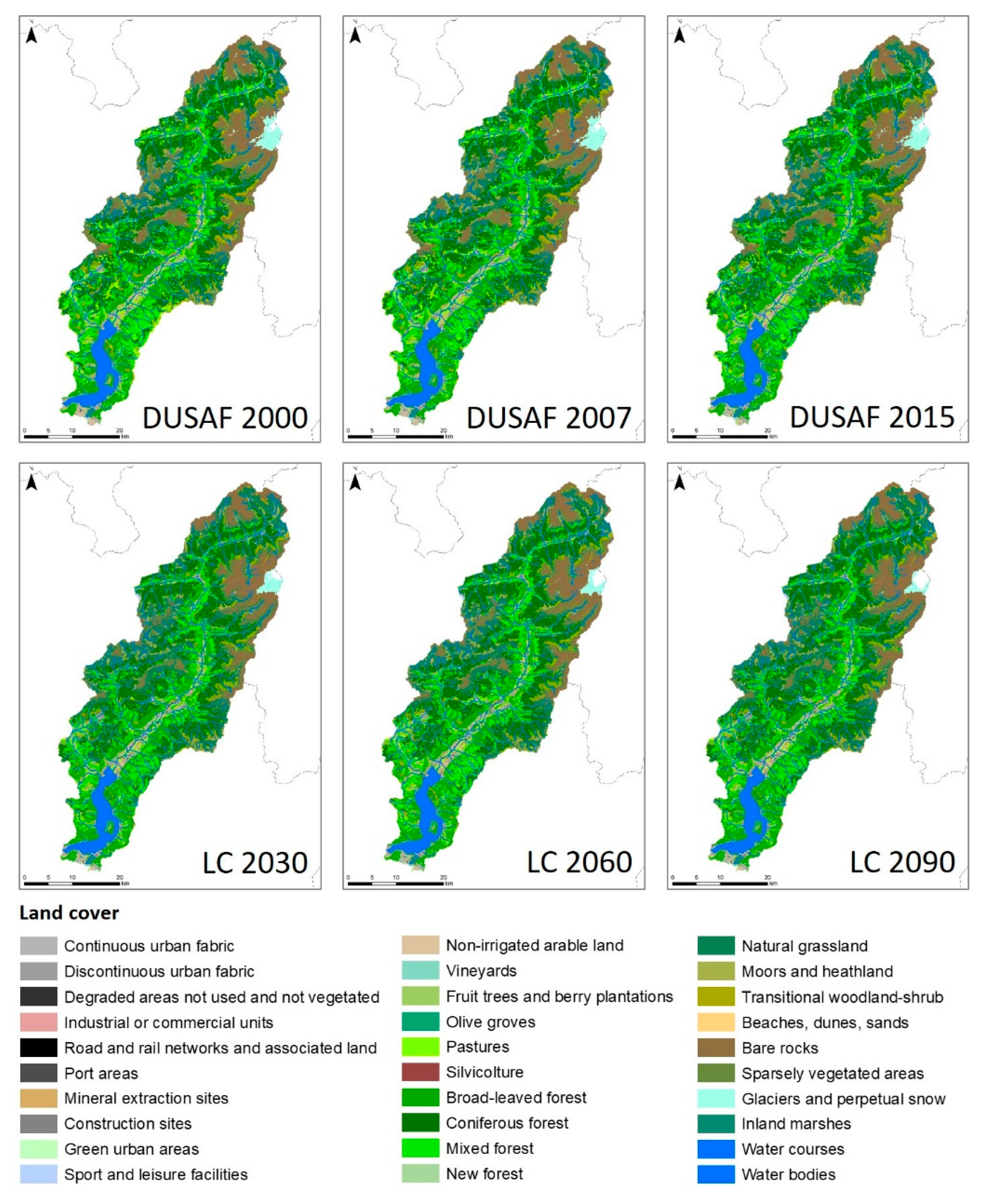
First, we quantified the land cover changes that occurred in the past with a classic change detection analysis between DUSAF 2000 and DUSAF 2015. To avoid meaningless changes, we retained only class transitions with a total geographic extension larger than 3000 cells (i.e., more than 2.7 [km
2]). This analysis highlighted 16 main land cover transitions and 7 main land cover persistences, which were grouped in the three sub-models reported in
Table 1.
Then, for each of the three sub-models we built a multi-layer perceptron neural network (MLP-NN). All the MLP-NNs were designed with three input neurons (elevation, slope, and aspect) and a hidden layer with six neurons. The output layer used to predict the probability of land cover changes in the future had as many neurons as the number of potential land cover transitions and potential land cover persistences (5 for sub-model #1, 9 for sub-model #2, and 11 for sub-model #3).
Figure 3 shows the neural network design.
The third step was the training of the networks (one for each sub-model) to set the optimal weights (). A set of training data and a set of testing data were automatically extracted from the reference land cover maps. To avoid sub-optimal solutions or an unstable training process, we used a learning rate of 0.0001. Moreover, we used a momentum of 0.5 for increasing numerical stability and for reducing volatility over the training epochs.
Once trained, the neural networks were used to generate a set of land cover transition/persistence potentials [
44]. Finally, using the past land cover changes and the modelled transition/persistence potentials, the future land cover map was predicted with a Markov Chain. Specifically, having evaluated the historical land cover changes from time t
1 to time t
2, the Markov Chain estimated the portion of land that is expected to transition from one class to another other, between the time t
2 and a future time t
3 [
46].
By repeating the process mentioned above, we simulated one land cover (LC) map for each of the 30-years simulation period: LC 2030, LC 2060, and LC 2090. For limiting error propagation in the simulation process, the MLP-NNs were trained with at least one real land cover map (i.e., DUSAF). Therefore, for the simulation at year 2030 the networks were trained with the DUSAF 2000 and DUSAF 2015 maps, DUSAF 2007 and the simulated land cover map for year 2030 (LC 2030) were used for predicting the land cover at year 2060 (LC 2060), and DUSAF 2015 and the simulated map at year 2060 (LC 2060) were used for the last prediction at year 2090 (LC 2090). Moreover, since initialization of the neural network is prone to numerical issues, we repeated each simulation five times, for a total of 15 simulations for every 30-years period. The final land cover maps were generated by retaining the modal value of each land cover simulation. While this is not a Monte Carlo simulation, however the multiple repetitions allowed us to get a more accurate prediction of the future land cover, minimizing the intrinsic error of the single stochastic simulation.
3.5. Projections of Future Cover Management Factor
As a result of our simulations, we described the dynamics of the cover management factor through the following land cover maps:
1981–2010 (reference period): DUSAF 2000 map;
2011–2040: simulated LC 2030 map;
2041–2070: simulated LC 2060 map;
2071–2100: simulated LC 2090 map.
Clearly, future projections of the cover management factor cannot exploit the satellite observations for reproducing the seasonal dynamics of vegetation. Thus, the cover management factor was estimated by assigning a fixed value to land cover classes at each simulation period (
Table 2) [
35,
47]. This means that our simulations only considered the trend of the C-factor and were not able to reproduce its seasonal variability.
4. Results
4.1. Projections of Precipitation, Temperature, and Rainfall Erosivity
Comparing the simulated mean annual precipitations at the rain gauges (2003–2017) with observations (2003–2017), we found the following biases in the downscaling process: 3.7% for ECHAM6, 3.9% for EC-Earth, and 4.5% for CCSM4. In the same period, at the thermometers the biases were: 0.1 °C (ECHAM6 and EC-Earth) and 0.0 °C (CCSM4).
Among the nine climate scenarios, GCM CCSM4 driven by RCP4.5 projected the smaller changes for annual precipitation (−1.8%) and temperature (+1.4 °C) at 2071–2100. On the other hand, GCM EC-Earth driven by RCP8.5 projected the larger changes for annual precipitation (+8.4%) and temperature (+4.0 °C) at 2071–2100. For this reason, our analysis focused only on these two extreme scenarios: GCM CCSM4 driven by RCP4.5 (hereafter referred to as SIM#4.5) is our best-case scenario and GCM EC-Earth driven by RCP8.5 (hereafter referred to as SIM#8.5) is our worst-case scenario. All the other scenarios lie in the between.
Figure 4 shows a comparison between the 30 m spatialized mean annual observed vs. simulated precipitation and temperature in the period 2003–2017. On the one hand, precipitation was slightly underestimated in all the domain. On the other hand, observed and simulated temperatures show a good agreement, being characterized by a negative gradient with elevation.
Table 3 and
Table 4 summarize the numerical results.
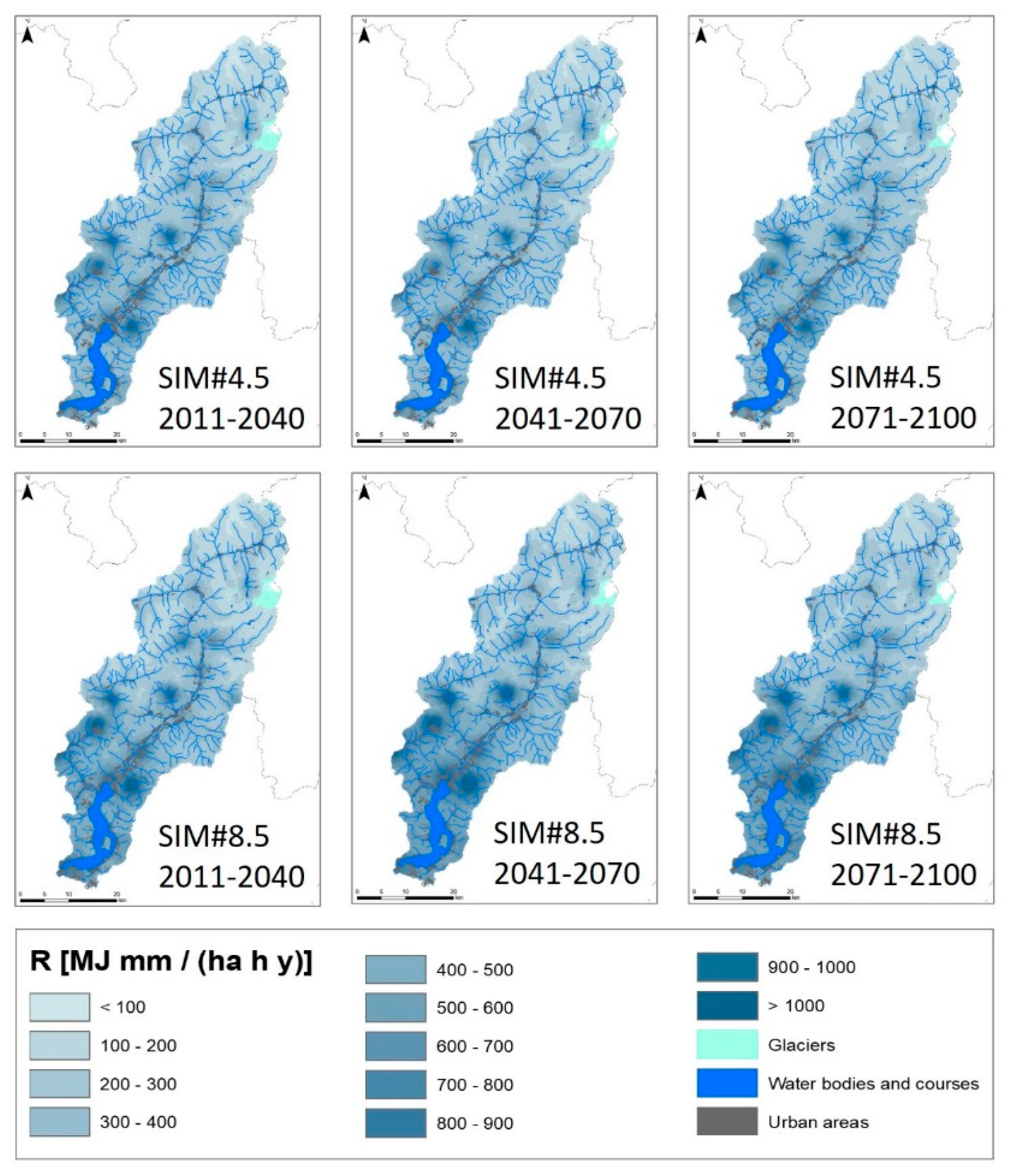
Figure 5 and
Figure 6 report the mean precipitation and temperature anomalies simulated with SIM#4.5 and SIM#8.5 at 2011–2040, 2041–2070, and 2071–2100. The baseline is the reference simulated period (1981–2010).
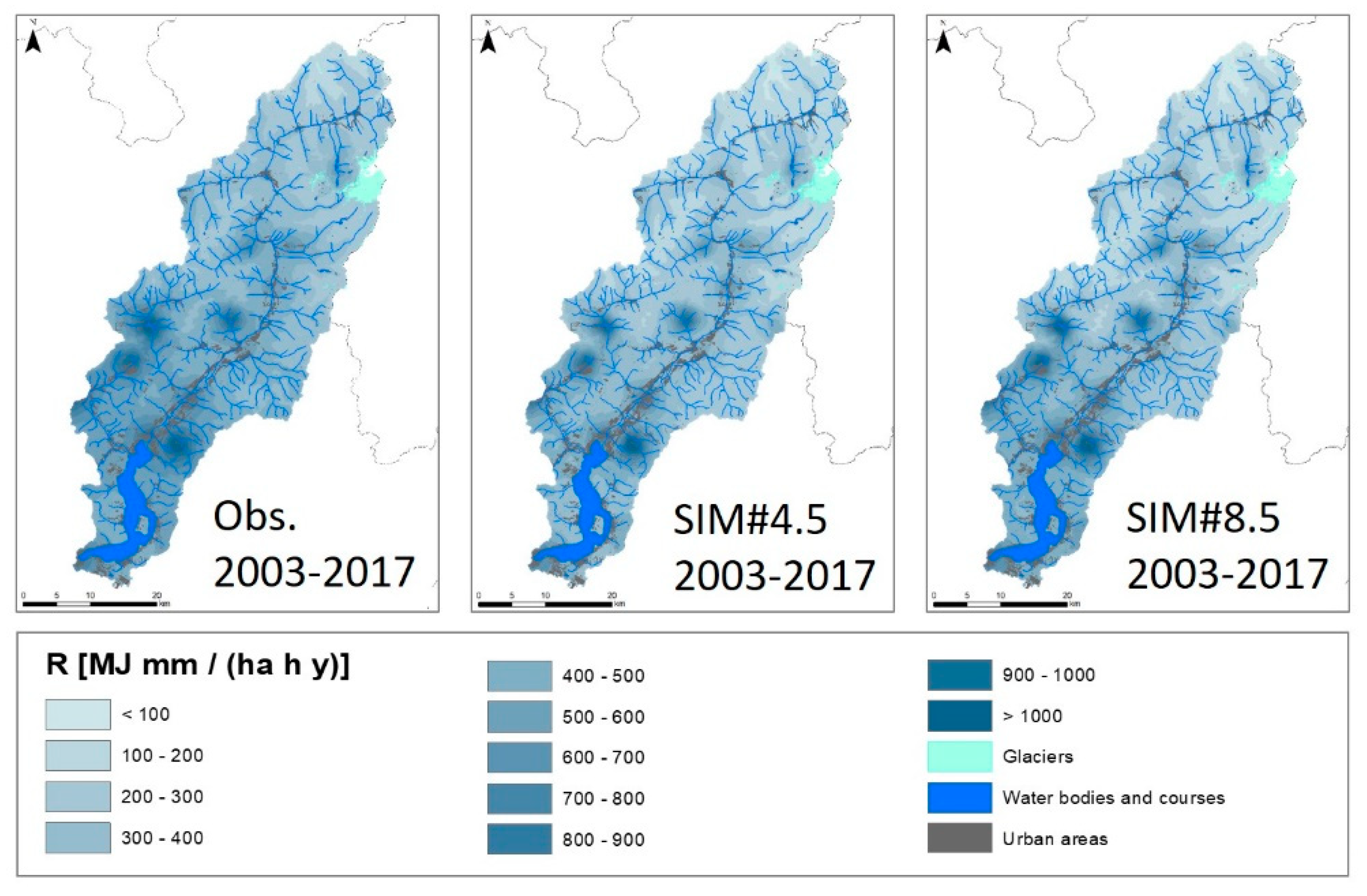
Figure 7 shows a comparison between the spatialized R-factor based on observations vs. simulations for the period 2003–2017.
Figure 8 reports the projections for SIM#4.5 and SIM#8.5. The simulated maps show spatial patterns that are similar to those observed but the R-factors are underestimated by about 26% in both SIM#4.5 and SIM#8.5 (
Table 5).
4.2. Projections of Future Land Cover and Cover Management Factor
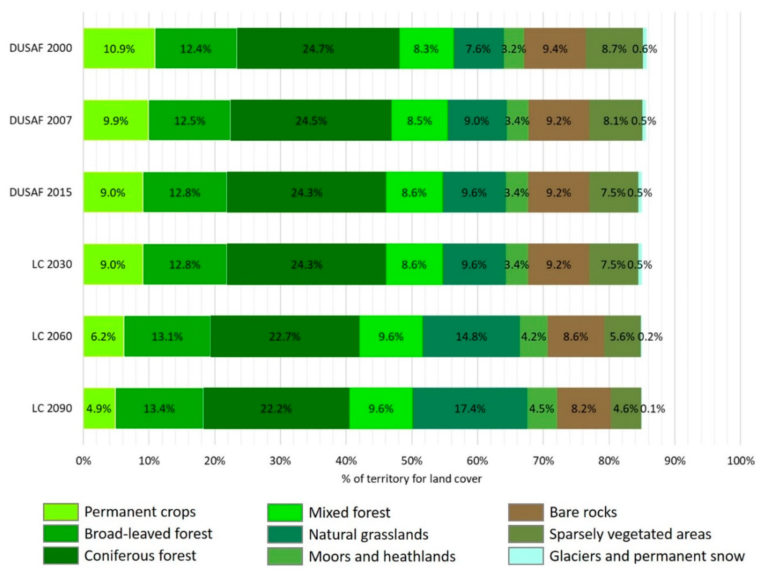
The change detection analysis of past land cover (
Figure 9 and
Figure 10) revealed that sparsely vegetated areas and pastures respectively reduced by 14% and 17%. They were almost replaced by natural grasslands, which increased by about 27%, and by moor and heathlands, which increased almost 8%. On the other hand, transitional woodland-shrubs, bare rocks, glacier and perpetual snow areas remained almost stable.
With reference to future land cover simulations, results show the following temporal trends (
Figure 9 and
Figure 10):
Sparsely vegetated areas and pastures continue to reduce almost constantly until 2090;
Natural grasslands continue to increase almost constantly until 2090;
Moors and heathlands show a rapid increase until 2060 and then a slower increase until 2090;
Transitional woodland-shrubs and bare rocks show respectively a minimal increase and a minimal decrease in the simulation periods;
Glacier and perpetual snow considerably reduce (from −37% in the first 30-years period to
−52% in the third 30-years period), in accordance with the expected retreat of the Adamello glacier and the disappearance of the Ortles glacier.
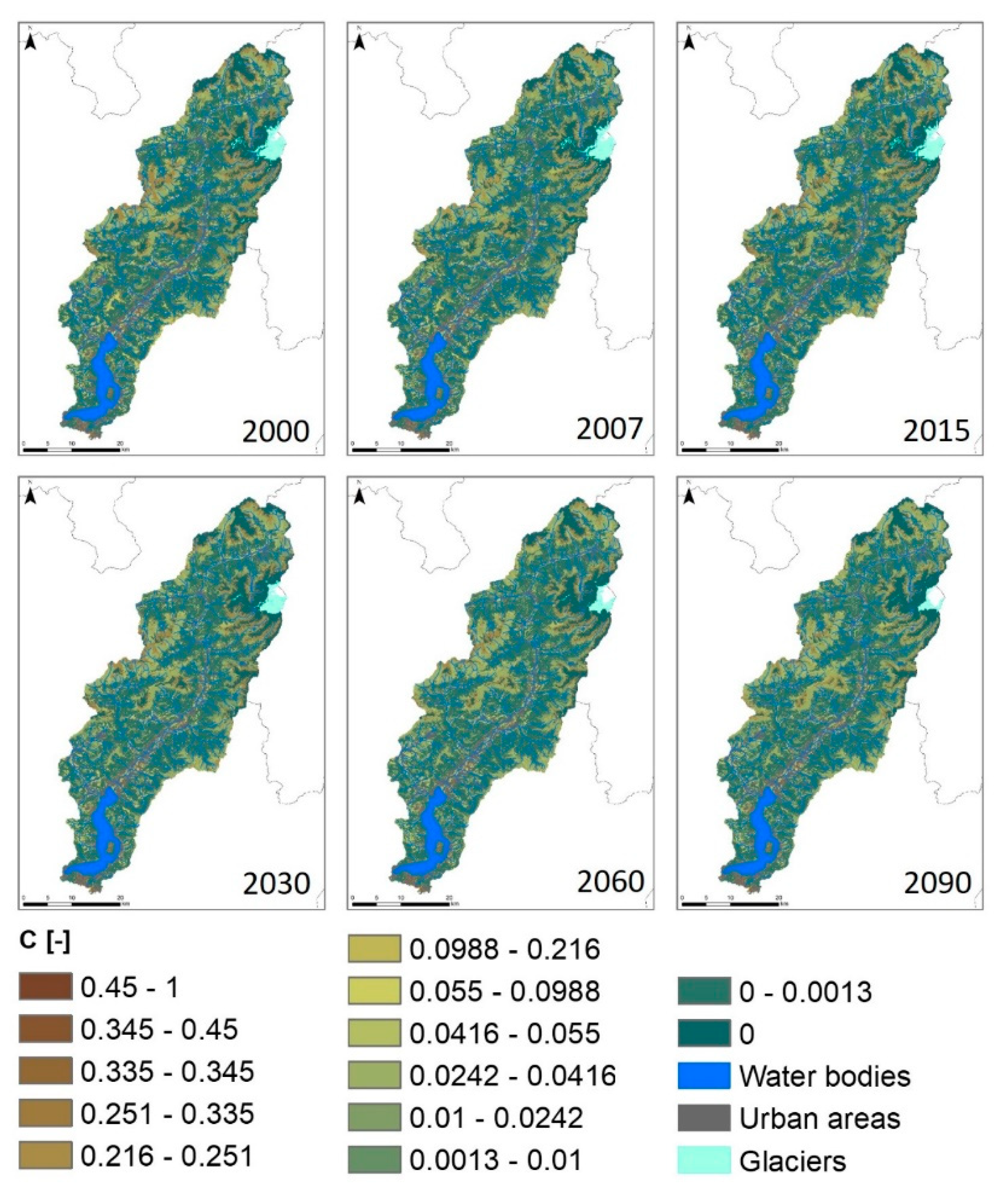
Consequently,
Figure 11 shows the dynamics of the C-factor computed with the observed land cover maps (DUSAF 2000, DUSAF 2007, DUSAF 2015) and the projected C-factor computed with the future land cover maps (LC 2030, LC 2060, LC 2090). Overall, projections show a gradual decrease of the mean C-factor for the whole study area (from 0.046 in 2000 to 0.033 in 2090), thus a gradual increase in the sheltering effect of vegetation cover toward soil erosion. The same result occurs when analyzing the three regions separately (from 0.052 to 0.035 for the North region, from 0.045 to 0.034 for the Center region, and from 0.040 to 0.030 for the South region).
4.3. Effect of Climate Projections on the Estimates of Soil Erosion
To evaluate the effects of climate change on soil erosion, independently from land cover changes, we run our simulations with a static land cover. In this case, we used the DUSAF 2015 for the whole simulated period (1981–2100). The erosion scenarios obtained with static land cover are hereafter referred to as SIM#4.5_D2015 and SIM#8.5_D2015, depending on the climate scenarios used.
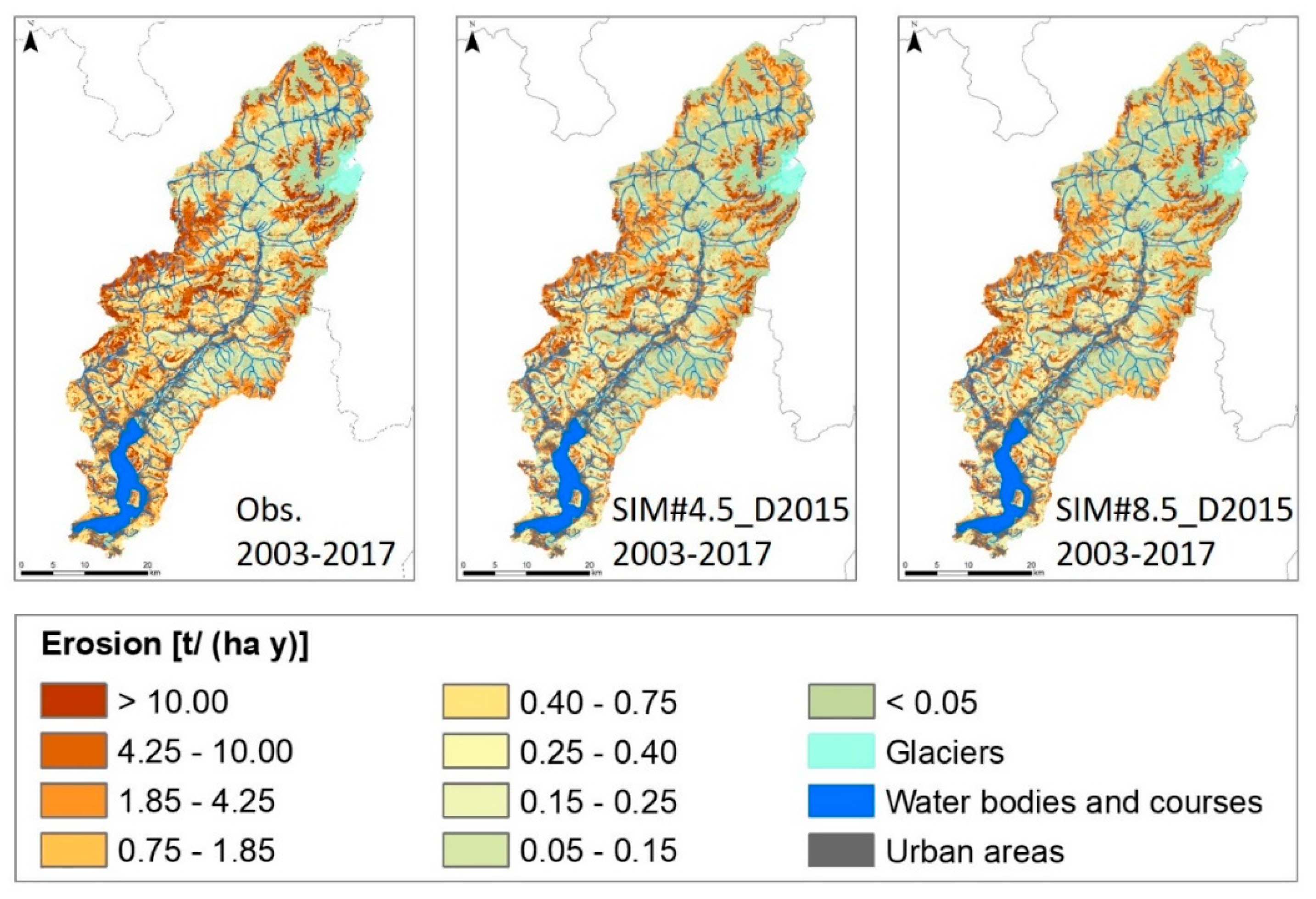
Figure 12 presents the comparison of observed [
35,
47] vs. the simulated mean annual soil erosion rates for the period 2003–2017 and using the two climate scenarios SIM#4.5 and SIM#8.5. The simulated maps show spatial patterns that are similar to those observed, but the erosion rates are underestimated of about 29% in SIM#4.5_D2015 and 44% in SIM#8.5_D2015 (
Table 6). As already mentioned, the overall underestimation is strictly related to the underestimation of the R-factor in the same period.
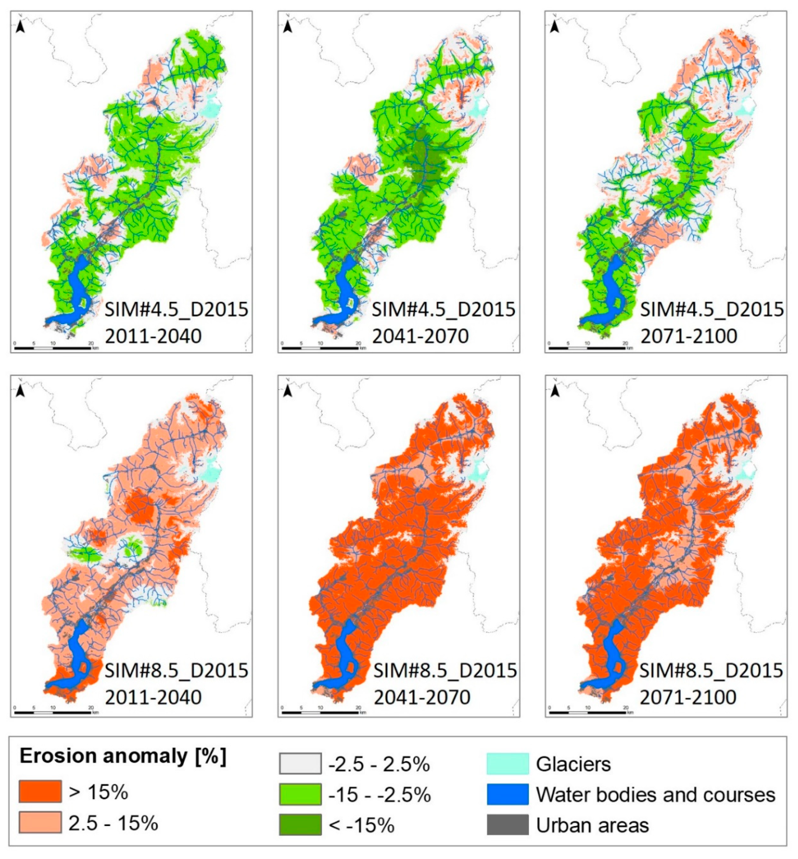
More in details,
Figure 13 reports the projected changes of erosion rates (baseline 1981–2010). Under the hypothesis of a static land cover, changes in erosion rates are only due to rainfall erosivity variability as stated in Equation (1). Expected mean erosion rates for the periods 2011–2040, 2041–2070, and 2071–2100 are detailed in
Table 7.
According to SIM#4.5_D2015, the mean erosion rate of the study area is expected to remain almost constant. The Center region, on average, has the highest erosion rates, while the North region has the lowest rates.
SIM#8.5_D2015 foresees a different scenario: the mean erosion rate of the study area is expected to grow until 2070, and then stabilize. In this case, the territory with the highest erosion rates is the South region, while the North region shows the lowest rates. As expected, the erosion rates predicted by SIM#8.5_D2015 and averaged on the study area exceed those of SIM#4.5_2015 by 8% for the simulation period 2011–2040, by 28% for the simulation period 2041–2070 and by 23% for the simulation period 2071–2100.
Finally,
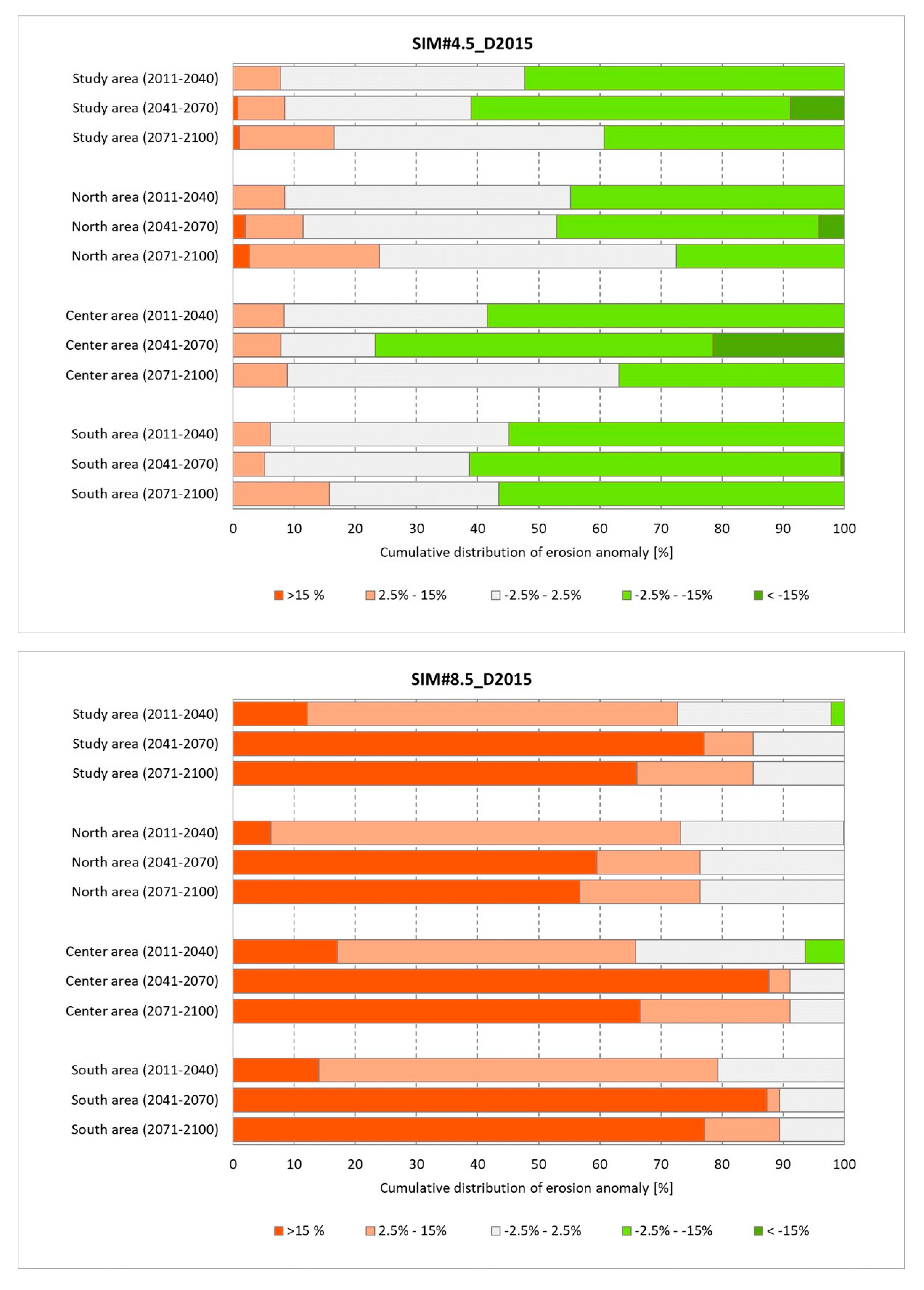
Figure 14 summarizes the percentages of the study area and regions where erosion is predicted to increase, decrease, or remain stable.
4.4. Combined Effects of Climate and Land Cover Projections on the Estimates of Soil Erosion
To evaluate the combined effects of climate and land cover changes, we run our simulations with a time-dependent land cover. In this case, we used LC 2030 as representative for the 30-year period 2011–2040, LC 2060 as representative for the 30-year period 2041–2070 and LC 2090 as representative for the 30-year period 2071–2100. For the control period (1981–2010) we assumed the observed land cover given by DUSAF 2000. The erosion scenarios obtained by combining the two climate scenarios with dynamic land cover are hereafter referred to as SIM#4.5_LC and SIM#8.5_LC.
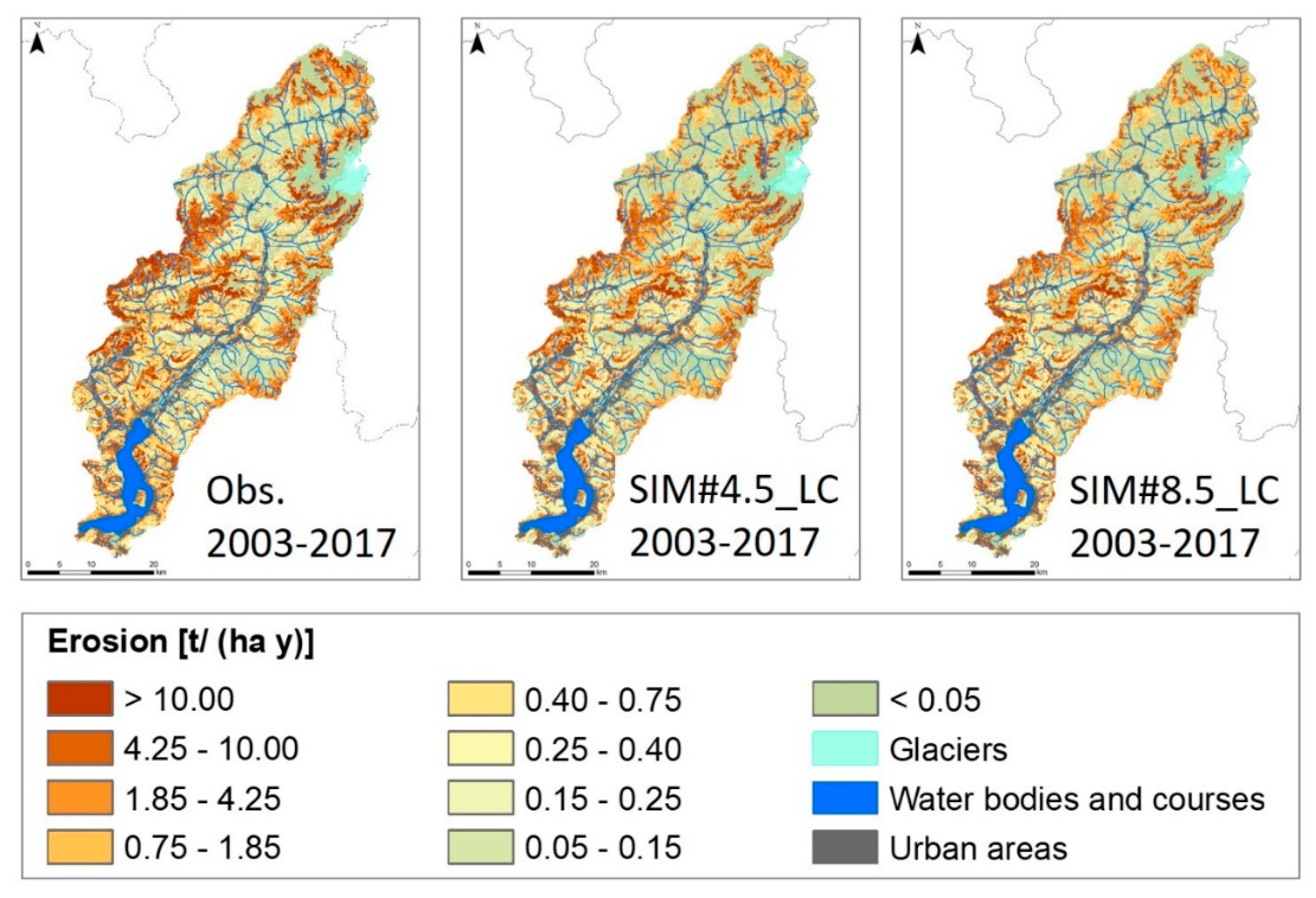
Figure 15 shows the comparison of observed [
35,
47] vs. simulated mean annual soil erosion rates for the period 2003–2017 and extracted from those generated from the erosion scenarios SIM#4.5_LC and SIM#8.5_LC. The simulated maps show spatial patterns that are similar to those observed, but the erosion rates are still underestimated (
Table 8). Nevertheless, the better performances of SIM#4.5_LC vs. SIM#4.5_D2015 and of SIM#8.5_LC vs. SIM#8.5_D2015 (
cf. Table 3 and
Table 8) are due to the land cover dynamics (i.e., DUSAF 2000 from 2003 to 2010 and LC 2030 from 2011 to 2017).
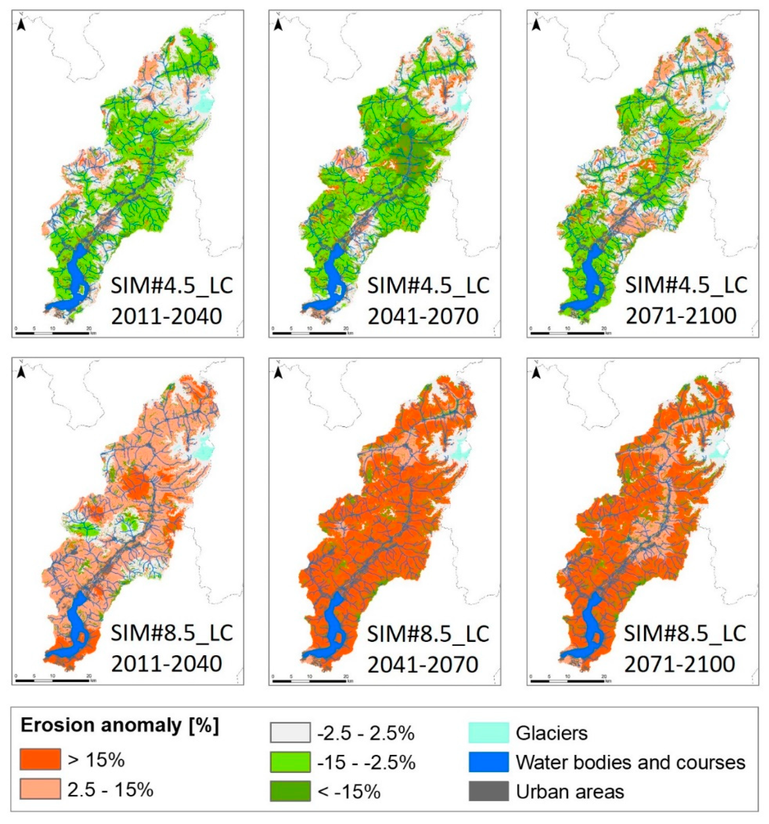
Figure 16 shows the maps of soil erosion rate anomaly for the thirty-year periods 2011–2040, 2041–2070, and 2071–2100 under the hypothesis of changes in both climate and land cover. The expected mean erosion rates are summarized in
Table 9.
The spatial patterns of future erosion anomalies (
Figure 15) are similar to those presented for SIM#4.5_D2015 and SIM#8.5_D2015 (
Figure 13), but with local variations because of the land cover changes. Overall, projections with land cover dynamics returned lower erosion rates compared to simulations with static land cover and, as expected, SIM#8.5_LC erosion rates averaged on the whole study area exceeded those of SIM#4.5_LC (by 7% for the thirty-year period 2011–2040, by 28% for the thirty-year period 2041–2070, and by 23% for the thirty-year period 2071–2100).
According to SIM#4.5_LC, the mean erosion rate on the study area is expected to slightly decrease. On average, the Center region will have the highest erosion rates, while the North region will have the lowest erosion rates. Conversely, according to SIM#8.5_LC the study area is expected to slightly increase the mean erosion rate from the first (2011–2040) to the second thirty-year period (2041–2070), and then slightly decrease in the last thirty-year period (2071–2100). In this case, the highest erosion rates are in the South region, while the North region shows the lowest rates.
Overall, both SIM#4.5_LC and SIM#8.5_LC project a decrease in the mean soil erosion rate and these trends seem contradicting the positive anomalies shown in
Figure 16. Finally,
Figure 17 summarizes the percentages of the study area where erosion is predicted to increase, decrease, or remain stable.
5. Discussion
Taking into account the different spatial domain and the different models used for climate change projections, our simulated mean increase in rainfall erosivity (+24% by 2040) is in line with the overall estimate for Europe (+18% by 2050) made by the European Commission [
50]. Nevertheless, land cover transformations could modulate (mitigating or enhancing) some erosional trends. Thus, the counterbalancing effects of both precipitation and land cover dynamics will be considered when predicting future trends to avoid inaccurate predictions at local scale.
Our results clearly show that both climate and land cover changes contribute to modifying future soil erosion rates. On the one hand, for static land cover, when simulating the climate change with the worst-case SIM#8.5_D2015 scenario we see a growth of the areas with increasing soil erosion and a gradual regress of the areas with decreasing soil erosion. On the other hand, when comparing the same climate scenario with and without the land cover evolution (i.e., SIM#4.5_D2015 vs. SIM#4.5_LC or SIM#8.5_D2015 vs. SIM#8.5_LC), we see a decrease in the mean soil erosion rate over the whole study area because of an enhanced sheltering effect by vegetation and the retreat of glaciers, which compensates for the increase of rainfall erosivity. Nevertheless, the spatial extent with enhanced erosion anomalies with higher (positive and negative) erosion anomalies expand.
Results show that a critical point is the capability of the climate scenarios to correctly simulate the occurrence and the intensity of the precipitation events: biases in the precipitation intensity cause a general underestimation of the R-factor in the reference period, even if the annual mean precipitation is well reproduced. Therefore, the variability of climate projections results in the absence of a clear direction of change of erosion rates that seems more influenced by the temperature increase rather than by precipitation trend. Specifically, the expected temperature increase will cause an increase in rainfall erosivity because snowfall is expected to diminish and rainfall is expected to increase, even if the annual precipitation (i.e., rainfall+snowfall) does not change significantly.
5.1. Projections of Precipitation
Considering the first thirty-year period (2011–2040), the SIM#4.5 climate scenario predicts that precipitation will slightly increase (between +2.5% and +15%) in 17% of the study area and will slightly decrease (between -15% and -2.5%) in the 3% of the of the study area. More in detail, this scenario returns that:
North: 5.5% of this territory will have a slight increase, 9.0% will have a slight decrease and the rest will have almost constant precipitation;
Center: 19% of this territory will have a slight increase and the rest will have almost constant precipitation;
South: 25% of this territory will have a slight increase and the rest will have almost constant precipitation.
Over the same period, the SIM#8.5 climate scenario predicts a slight increase for 99% of the study area and a moderate increase for the remaining 1%, mostly located in the Center (overall about 2.4% of Center region).
Considering the second thirty-year period (2041–2070), SIM#4.5 predicts that precipitation is expected to slightly decrease in 97% of the study area, and all the three regions show the same trend. On the other hand, SIM#8.5 predicts a different signal over the same period; about half of the study area (48%) will have a slight increase, and about half of the study area (52%) will have a moderate increase. More in details, the slight increase of precipitation is expected in 88% of the North region, 34% of the Center region, and 15% of South region, while the moderate increase will affect 12% of the North region, 66% of the Center region, and 85% of South region.
Considering the last thirty-year period (2071–2100), SIM#4.5 predicts that the majority of the study area (91%) will have almost constant precipitation and only 9% a slight decrease. In this case, the precipitation reduction is foreseen in 15% of the North region, 8.4% of Center region, and 2.4% of South region. Over the same period, SIM#8.5 projects a slight increase in precipitation for the whole study area.
5.2. Projections of Temperature
According to SIM#4.5 (
Figure 6), the mean annual temperature is expected to change almost homogenously on the whole study area. The mean projected changes of temperature are +0.79 °C for 2011–2040, +1.48 °C for 2041–2070, and +1.42 °C for 2071–2100. In the period 2071–2100, our simulation shows a temperature anomaly decreasing from the South region (+1.44 °C) to the North region (+1.40 °C), while the valley floor that crosses the study area from North-West to South-East displays a higher temperature anomaly compared to its surroundings.
The SIM#8.5 climate scenario depicts a different picture: The mean projected changes of temperature are +0.62 °C for 2011–2040, +2.02 °C for 2041–2070, and +4.06 °C for 2071–2100. In the period 2071–2100, our simulations show a temperature anomaly decreasing from the North (+4.13 °C) to the Center (+4.05 °C) to the South (+3.99 °C). In this scenario, the northeastern of the North region, the western part of the Center region and the valley floor have the lowest temperature anomalies.
5.3. Simulation of Rainfall Erosivity
The spatial distribution of the simulated R-factors for 2003–2017 are similar to those estimated from observations in the same period (
Figure 7). However, as already pointed out, both simulations underestimate the rainfall erosivity by about 26%. A more detailed analysis revealed that the climate scenarios returned different results at local scale (
Table 5):
North: the bias is +5% for SIM#4.5 and −33% for SIM#8.5;
Center: the bias is −29% for both SIM#4.5 and SIM#8.5;
South: the bias is −23% for SIM#4.5 and −17% for SIM#8.5.
Overall, the underestimation of the rainfall erosivity might be related to differences in the sequence and intensity of the observed and simulated precipitation events, which are further emphasized by the quadratic relationship between hourly rainfall intensity and R-factor (Equation (2)). The stochastic generator used to downscale the simulated precipitation, by its nature, reproduces second-order statistics (i.e., mean and variance) of the observed dry/wet spell sequence and of mean daily precipitation. However, it does not replicate path-wise the observed precipitation patterns. This is consistent with the aim of projecting future precipitation patterns by downscaling IPCC projections, which are statistically consistent with the current, yet including modified climate change effects as projected.
According to SIM#4.5 the mean R-factor of the study area is expected to be almost constant (
Figure 7), with simulated values of 312 [MJ mm ha
−1 h
−1 yr
−1] in 2011–2040, 302 [MJ mm ha
−1 h
−1 yr
−1] in 2041–2070, and 316 [MJ mm ha
−1 h
−1 yr
−1] in 2071–2100. SIM#8.5 envisage a different scenario: the mean R-factor is expected to reach its maximum by 2041–2070 (400 [MJ mm ha
−1 h
−1 yr
−1]).
5.4. Projections of Future Land Cover and Cover Management Factor
The apparent disagreement between the trends predicted by SIM#4.5_LC and SIM#8.5_LC (
Figure 15), which project a decrease of the mean soil erosion rates, and the positive erosion anomalies (
Figure 16) is due to the small areas with large changes in C-factor estimates. In fact, the land cover evolution from DUSAF 2000 to LC 2090 projects that about 16% of the whole study area will see a reduction of C-factor. More than 55% of the land classified as “sparsely vegetated areas,” “pastures,” and “non-irrigated arable land” in DUSAF 2000 are modelled to evolve into land cover classes with lower C-factor. Thus, even local changes in land cover might have a big influence on the mean erosion rates of the whole study area. Specifically:
“Sparsely vegetated areas” cover 8.7% of the study area in 2000 (it is the third more frequent land cover) but are projected to reduce to 4.6% in 2090;
“Pastures” cover 10.9% of the study area in 2000 (it is the fifth more frequent land cover) but are projected to reduce to 4.9% in 2090;
“Non-irrigated arable land” covers 1.1% of the study area in 2000 but is projected to reduce to 0.7% in 2090.
Result strongly depends on the reliability of the land cover simulation process but, unfortunately, there are few chances to assess its real accuracy. An exception is the simulated land cover map for the thirty-year period 2011–2040 (LC 2030) because the neural networks was trained using the observed land cover (DUSAF) for both the periods (2000 and 2015). The weighted skill score (Equation (5)) used to evaluate the projected land cover map is similar to the Cohen’s kappa statistic, where the expected accuracy by chance is estimated as the same chance of happening (Equation (6)):
where:
is the skill score for the sub-model i;
is the measured accuracy of the transition/persistence for class j for the sub-model i;
is the expected accuracy of the transition/persistence for class j for the sub-model i;
is the percentage of land cover class j for the sub-model i;
is the number of transitions in the sub-model i;
is the number of persistence classes in the sub-model i.
Overall, the weighted skill score shows a moderate agreement for the sub-models #1 (S = 0.43) and #3 (S = 0.30), but no agreement for the sub-model #2 (S = 0.03). That could be due to the very short span of time considered for training the models (only 15 years), which seems not enough for defining the reliable trends in land cover changes. Nevertheless, that was the best option for our study area.
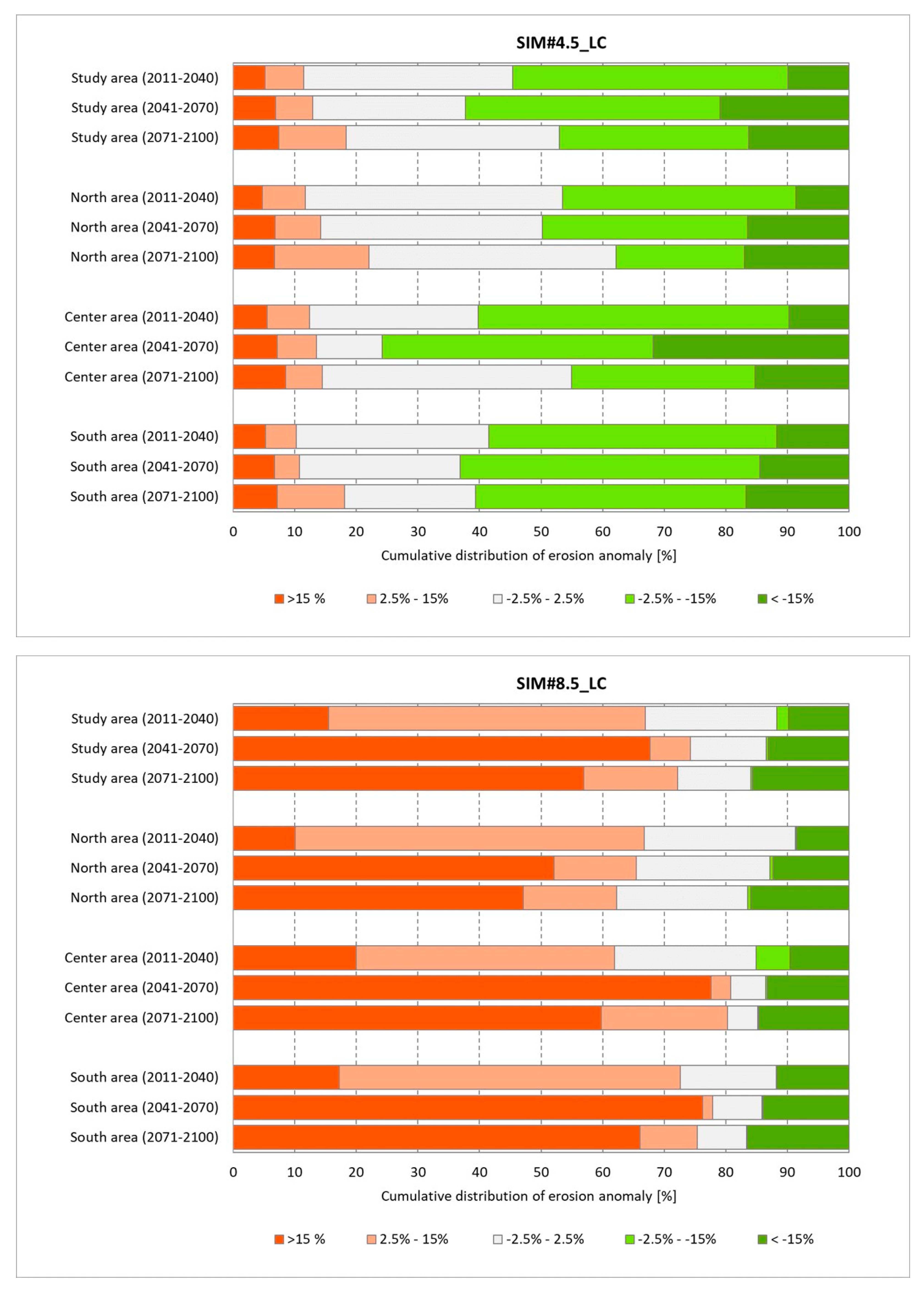
5.5. Estimates of Future Soil Erosion
With respect to static land cover simulations, SIM#4.5_D2015 foresees an erosion scenario with limited variability on the whole area: about 90% of the study area will have no changes or a slightly decrease in erosion rates. Only a small portion of the study area (7.7% in 2011–2040, 8.0% in 2041–2070, and 15.5% in 2071–2100) will see a slight increase in the erosion rates, mostly in the South and North regions. On the other hand, SIM#8.5_D2015 foresees a different scenario: most of the study area (72.7% in 2011–2040, 77.1% in 2041–2070, 85.1% in 2071–2100) will increase its erosion rates and the rest is expected to remain stable. This erosion scenario does not predict any decrease of erosion rates.
When combining climate with the land cover projections, SIM#4.5_LC foresees a similar scenario to SIM#4.5_D2015. However, in this case a smaller part of the study area is predicted to have no changes or a slight decrease in erosion rate (78.6% in 2011–2040, 66.1% in 2041–2070, and 65.3% in 2071–2100), and a larger part of the study area will see an increase in erosion rates (11.5% in 2011–2040, 13.0% in 2041–2070, and 18.4% in 2071–2100). In the rest of the study area, the soil erosion is expected to decrease moderately. As for SIM#4.5_DUSAF2015, the regions more exposed to soil erosion increase are the South and North.
Alike SIM#8.5_D2015, when considering land cover dynamics SIM#8.5_LC foresees an erosion scenario where most of the territory is supposed to increase its erosion rates. However, contrary to the static land cover simulation, SIM#8.5_LC highlights some local areas where soil erosion moderately decreases due to land cover changes.
5.6. Comparison to Similar Studies
Although a common belief is that increased rainfall amounts and intensities will lead to greater erosion rates, it is rather difficult comparing our findings with existing literature. The reason is that different studies have substantial differences in:
Working scale. The majority of papers performs global, national, or regional analysis, and not local-scale analysis;
Topographic and land cover characteristics of the study areas;
Model used to estimate soil erosion;
Model used to project climate and land cover changes.
Even with these limitations, our study complements the existing literature on the synergic effects of climate and land cover change on soil erosion.
In their review about studies of potential effect of climate change on soil erosion rates at a national scale (USA), Nearing et al. [
11] reported that, unless amelioration measures were taken, erosion will increase (with significant geographic heterogeneity) mainly as function of an increase in rainfall amounts and intensities, rather than the number of days of precipitation in a year. In this review, erosion and runoff rates were mainly computed with the Water Erosion Prediction Project (WEPP) model [
51] and changes in rainfall erosivity were determined according to estimations of future climate change provided by two GCMs through statistical relationships. Moreover, where rainfall amounts were projected to increase, erosion and runoff were expected to increase at an even greater rate (the ratio of erosion increase to annual rainfall increase is approximately 1.7). Although not predicting land cover changes, the authors declared that even in cases where annual rainfall would decrease, systems feedbacks related to decreased biomass production could lead to greater susceptibility of the soil to erosion.
A more detailed study by Zhang et al. [
14], evaluated the potential impacts of precipitation changes on soil erosion and surface runoff in southeastern Arizona. The authors used seven GCMs models, three emission scenarios for the 2050s and 2090s and the Rangeland Hydrology and Erosion Model (RHEM) described in [
52]. The seven models used show a similar variability in the annual precipitation for all the three scenarios, ranging from −17.9 to +13.7%. However, a decreased biomass production could lead to long-term increase in soil erosion due to sparser vegetation cover [
11]. In this case, the authors expected an increment of soil erosion between +44.7 and +210.4%, depending on the models and scenarios considered. The authors also claimed that future increase in runoff and soil erosion could accelerate the transition of grassland to shrubland, or to more eroded states, due to the positive vegetation-erosion feedback.
Other authors [
15,
16,
17,
18] evaluated the long-term impact of climate change on sediment yield and soil erosion for the Mediterranean region, projecting future climate to 2100. These studies demonstrated that estimated erosion variations can be closely related to changes in precipitation and temperatures, although a biomass growth could be significant in determining the climate change impacts on erosion. However, there is a wide spatial variability in the trends for soil erosion depending on rainfall changes and biomass growth and relevant uncertainty still characterize these types of works.
The analysis of the combined effect of both climate and land cover changes is more common at a local scale. Asselman et al. [
19] studied the potential effects of changes in both climate and land use on sediment transport from the upstream basin to the lower Rhine delta. In this case, the authors considered three climate change scenarios based on the UK Hadley Centre’s high-resolution atmospheric general circulation model [
53], corresponding to a temperature rise at 2100 of +1 °C, +2 °C, and +4 °C. Considering the intermediate climate change scenarios, the authors estimated across the entire Rhine basin a temperature rise from +3.2 °C to +3.9 °C in summer and from +4.3 °C to +4.5 °C in winter. While precipitation changes were projected from -9.8% to 10.9% in summer and from +16.6% to +32.7% in winter. In addition, they considered two land use change scenarios that forecast a decrease in crop production because of population growth, and a considerable reduction of the agricultural land because of temperature and CO
2 concentration increase. Soil erosion was estimated with the Rhine model for evaluating the effects of Environmental Change On Delivery of Eroded soil to Streams (RECODES) described in [
54], which is based on the Universal Soil Loss Equation (USLE) model [
55]. Their findings showed that, for the projected climate and land use changes, erosion rates were expected to increase in the Alps and to decrease in the German part of the basin, with a mean increase of +12% for the Rhine basin.
Serpa et al. [
13] analyzed the impact of climate and land use changes on streamflow (water quantity) and erosion in humid (Sao Lourenco) and dry (Guadalupe) Mediterranean catchments in Portugal. They used the SWAT hydrological model [
56], which computes soil erosion through the Modified Universal Soil Loss Equation (MUSLE) model [
56]. Climate change scenarios were developed for the period 2071–2100 using the ECHAM5 GCM [
57] driven by two emission scenarios (A1B and B1) projecting a decrease in annual rainfall for both catchments (humid: −12%; dry: −8%), but a significant increase of rainfall in winter (+19% for Sao Lourenco and +40% for Guadalupe). Land use scenarios were defined from a linear downscaling of European trends for generic land use types in Portugal, improved by local trends estimated from a comparison with past land cover to identify possible land-cover type replacements. In their study, the authors also analyzed socio-economic trends to gain insight into the driving forces behind land use changes. They defined two scenarios, which both predicted a decrease in agricultural lands for food production. Their results showed that both climate and land cover changes strongly influence soil erosion and sediment transport in both the basins studied. However, they got contrasting results in estimations of sediment transport for the humid (A1B: −29%; B1: −22%) and dry (A1B: +222%; B1: +5%) catchments.
Molina-Navarro et al. [
20] published an application of the SWAT model in the Spanish area of the Ompólveda River catchment. They considered eight scenarios obtained by combining climate and land use projections. According to their findings, the increase of scrublands and forests were expected to reduce future soil erosion, while the increase of croplands could make the soil more prone to erosion.
Finally, the work by Routschek et al. [
21] investigated the future changes in erosion rates for three catchments in West, North, and East Saxony/Germany under climate and land use/soil management changes. The climate projection showed a slight increase of precipitation, with a decrease in the number of events with low intensities (0.1–0.2 [mm min
−1]) and medium intensities (0.2–0.5 [mm min
−1]). On the other hand, the number of rainstorms with high and very high intensities (>1 [mm min
−1]) was expected to increase. The authors concluded that, without proper soil management and land use policies, climate change will lead to an increase of soil loss by 2050 and a partial decrease from 2050 to 2100. Moreover, the authors also pointed out that changes in soil management such as “no tillage” or land use changes from agriculture to pasture/forest could reduce the soil erosion of more than 90%, thus with a much higher impact than that of climate change alone. This means that, according to [
21], land cover and use changes and soil management practices are expected to have higher impacts on soil erosion than precipitation patterns.
The analysis of existing literature has evidence that both climate change and land cover changes will have an impact on future soil erosion. Nevertheless, all past works highlight that projected soil erosion patterns could be very heterogeneous in the areas studied. Our research is substantially in line with these outcomes, confirming an overall increase of soil erosion in the Alps due to climate change, modulated by land cover changes which can generate local patterns of decreasing erosion. That makes very challenging the definition of a general trends.
5.7. Current Limitations
D-RUSLE is an empirical method for modelling potential erosion caused by the impact of raindrops. Thus, from the modelling point of view, erosion is mainly controlled by precipitation, land cover, topography, soil properties, and soil conservation practices. This means that, similar to any other erosion model derived from RUSLE, also D-RUSLE does not consider the melting of permafrost.
While the effects of permafrost should be very limited in the area studied, in other sites, latitudes or elevations, permafrost could play a very important role in controlling soil erosion. As a matter of principle, D-RUSLE could be modified for including a new parameter related to permafrost (the permafrost factor, PF-factor), but specific experimental activities and maps of the extension and dynamics of permafrost would be needed. That is beyond the scope of our research.
We are also aware that snow-induced erosion might be relevant in some mountain areas and RUSLE-like models cannot describe this effect [
58]. In D-RUSLE, the computation of R-factor includes the snow cover sheltering effect, thus simulating the snow accumulation and melting process, but our model neglects the erosion because of snow melting. Theoretically, snow melting could be included in the computation of the rainfall erosivity factor by considering the snow-water equivalent data (this is a different process from the raindrop action on soil simulated by RUSLE-like models). However, it might be complex to get a satisfactory conversion of snowfall into equivalent liquid precipitation because the snow cover usually has a significant spatial and temporal heterogeneity [
59] and the snow melting processes might show oscillations over time.
With respect to C-factor, currently unvegetated soils are given a null value, thus a null erosion regardless the rainfall intensity. This is a heritage of RUSLE-like modelling that seems reasonable for compact rocks but could be not true for the moraines exposed to the retreat of glaciers. Consequently, this parametrization is conservative and underestimates the soil erosion at higher elevations.
Finally, our study did not include land management policies as constraints for simulating future land cover transformations. Future refinements could might also consider this aspect.
6. Conclusions
Global warming, and its consequences on glacier retreat and frequency of extreme events, is now undeniable [
60]. Climate change and land cover transformations have gained increasing attention because of their impacts on the environment. In particular, they are considered to be the main causes of accelerated land degradation and, specifically, of soil erosion. Therefore, maintaining soil quality for achieving food security, acting to mitigate climate change, and restraining land degradation have been considered among the recently approved United Nations Sustainable Development Goals [
61].
This is the first study investigating the future scenarios of soil erosion under both climate and land cover changes in Val Camonica and Lake Iseo, one of the largest valleys of the central Alps. Specifically, we investigated nine climate scenarios until 2100 and then analyzed in detail the impacts of soil erosion on two of them: GCM CCSM4 driven by RCP4.5 and the GCM EC-Earth driven by RCP8.5. The first climate scenario forecast a best-case (and optimistic) temperature increase of +1.4 °C and small changes in annual precipitation (−1.8%) by 2100. The latter scenario forecast a worst-case temperature increase of +4.0 °C and also larger changes in annual precipitation (+8.4%). Future land covers were simulated using automatic machine learning based on past observed land changes.
Our outcomes confirm past findings: both climate change and land cover changes will have an impact on soil erosion. Nevertheless, it is impossible to describe a trend consistent throughout the study region or for the entirety of Europe’s Alps because the projected soil erosion patterns are contextual and heterogenous. Depending on the simulation scenario, if the mean annual precipitation does not change significantly and temperature increases no more than 1.5–2.0 °C, then about half of the study area will experience a decrease in its mean annual erosion rate and less than 20% will see an erosion increase. At the other extreme, if the mean annual precipitation increases more than 8% and the temperature increases more than 4.0 °C, then about three-quarters of the study area will see increase in annual erosion. What clearly emerges from the study is that areas with higher (positive and negative) erosion anomalies are expected to expand, and their patterns will be modulated by future land transformations.
With a doubt, land cover prediction could be improved but it is important to consider this parameter in future scenarios. When working with future climate scenarios, we have no real way to validate such models because they provide precipitation projections that are consistent with observed precipitation amounts, but do not truly replicate climate. Thus, we cannot determine whether most of the uncertainties stem from land cover projections or from the climate scenarios used.

 ,
, 


