Ecological Niche Models Reveal Climate Change Effect on Biogeographical Regions: The Iberian Peninsula as a Case Study

Abstract

How species are distributed on Earth depends largely on climate factors. Whenever these environmental conditions change, species tend to shift their distributions to reach more favourable conditions. Distinct sets of species similarly distributed (i.e., chorotypes) occur in biogeographical regions with homogeneous environmental conditions. Here, we analysed whether biogeographical regions are unstable over time (from the past to the future). We modelled the realised niche of amphibians and reptiles in the Iberian Peninsula in the present, and several past and future climate scenarios. Then, we used Jaccard’s index and the unweighted pair group method (UPGMA) to define the biogeographical regions. Our results suggest that the biogeographical regions of Iberian amphibians and reptiles changed greatly over time, due to the climatic changes between periods. Biogeographical regions composed of species with Atlantic affinities changed particularly, overall gaining suitable areas in past colder periods and losing suitable areas in warmer periods. The areas of refugia for amphibians over time corresponded to the most humid regions (north-west of the peninsula), while the most important areas for reptiles occur in the south and on the Atlantic coast. The identification of biogeographical patterns considering past climate changes is essential to better apply conservation measures.

1. Introduction

The current biodiversity crisis has led to an increasing interest in biogeographical studies attempting to understand the spatial patterns of species distributions, boosted by technological advances such as geographical information systems and remote sensing [1,2,3,4,5]. Much effort has been dedicated to analyse how species are distributed across space, and how they are organised in regions of similar characteristics (e.g., [6,7]). These so-called biogeographical regions are ecologically and geographically defined areas of the Earth, generally with homogeneous geologic and environmental conditions [5,8,9]. Biogeographical regions are composed of distinct assemblages of species and communities, known as chorotypes, with statistically similar distributions [8,9,10].

Biogeography is an old discipline, dating back to the time when naturalists such as Humboldt [11], Sclater [12] or Wallace [13] realised that the biota is divided into distinct geographical units [14]. Using distribution data of global mammal fauna, Wallace divided the world into six geographical units coinciding with the limits of tectonic plates [13,15]. More than a century after, the biogeographical units proposed by Wallace (1876) are still valid; they have nowadays improved substantially with better species distribution data and technological tools [14,15]. A major weakness of these early works was the roughly defined criteria for delineating the biogeographical units [16]. Since the first works, these criteria have been successively refined [14,16,17,18,19]. Currently, hierarchical cluster analysis using Jaccard’s index and the unweighted pair group method using arithmetic averages (UPGMA) is widely applied to define biogeographical units [10,16,20,21,22,23]. This method establishes statistical patterns and uses the similarity among areas to reveal natural spatial patterns, allowing the delineation of distinct regions [22,24]. However, the availability of species distribution data can still be a limitation when estimating biogeographical regions. Ecological niche models (ENMs; [10,25,26]) can overcome this problem.

ENMs are used to forecast species ranges when their distributions are not well known [27,28]. Therefore, biogeographical regions can be delimited using the results from ENMs instead of the species distribution data [16,29,30]. The greatest advantage of ENMs is their capacity to be extrapolated to other scenarios in space and time [31,32,33], allowing analyses of how biogeographical regions change over time. Biogeographical regions are indeed not static: they change as the environment changes [34]. As a consequence, they are vulnerable to climate change [35,36,37]. The evidence about the future effects of climate on the species biogeography is increasing [34,38,39,40,41,42]. Many studies have identified species range shifts due to climate change (e.g., [43,44,45,46,47,48]). It is assumed that these range shifts may affect the spatial patterns of biogeographical regions, such as the Mediterranean area, a biodiversity hotspot of global importance [49,50]. However, no studies thus far have analysed in detail how biogeographical regions follow climate changes from the past to the future. Therefore, the main aim of this work is to analyse whether biogeographical regions are unstable over time (from the past to the future), using amphibians and reptiles of the Iberian Peninsula as a case study. For this, we calculated the realised ecological niches (sensu Sillero [51]) of amphibians and reptiles in the Iberian Peninsula in current times and projected it to different past and future climate scenarios. Specifically, we aim to (1) determine amphibians and reptiles’ chorotypes in the Iberian Peninsula in the past, present and future, (2) determine changes on species richness (hotspots) in chorotypes over time, (3) analyse the expansion and retraction of species ranges over time; and (4) identify possible areas of refugia over time for amphibians and reptiles in the Iberian Peninsula. To our knowledge, this is the first attempt to analyse changes in biogeographical regions of amphibians and reptiles over time.

According to the distribution of amphibians and reptiles, the Iberian Peninsula can be divided into two regions, corresponding mostly to the Atlantic and Mediterranean regions [10,52]. Therefore, here, we hypothesise that: (1) the Atlantic region increases in extent during periods of cold weather; (2) the Mediterranean region increases in extent during periods of warm weather; (3) in the future, the Atlantic region will reduce in extent, while the Mediterranean region will increase; (4) the Atlantic region had a maximum extension during the Last Glacial Maximum.

2. Materials and Methods

2.1. Study Area: Iberian Peninsula

We selected the Iberian Peninsula (Figure 1) as a case study because (1) it is a hotspot of biodiversity [49]; (2) it is an area where amphibians and reptiles are strongly impacted by climate change [53]; and (3) it works as a close system thanks to its peninsular condition, separated from the rest of Europe by the Pyrenees. The Iberian Peninsula remained almost ice-free during glaciations, representing important refugia for many species and a source of endemism [29,54,55]. Numerous species with different ecological requirements co-occur in the transition area between the Atlantic and Mediterranean climates [40].

The Iberian Peninsula has a heterogeneous climate, influenced by both the Atlantic Ocean and the Mediterranean Sea, with a longitudinal gradient of precipitation and a latitudinal gradient of precipitation and temperature [56]. It encompasses two main biogeographical regions: the Mediterranean and Atlantic [57]. The Atlantic region extends along the northern coast, and it is characterised by a maximum of two consecutive arid months during the summer (the mean precipitation, P, of the warmest two months is larger than twice the mean temperature, T, of the warmest two months: P > 2T; [10,56,58]). The Mediterranean region encompasses almost all the remaining areas of the Peninsula (P < 2T) and constitutes a major biodiversity hotspot. Occasionally, a third biogeographical region is referenced: the Alpine region, which is located in the north-east of the Peninsula, in the Pyrenean region [57].

2.2. Species Data Sources

Amphibians and reptiles are ideal species models because they have a strong link with the environment and a low dispersal capacity [10]. Both groups are very vulnerable to climate change impacts because of their ectothermic physiology [10,29,40,53,59,60,61]. Indeed, climate change is likely to be a major cause of the decline in amphibians and reptiles [62,63]; for example, in Europe, most species may lose suitable areas by 2050 [29]. Iberian amphibians are mostly threatened by the increasing aridity, more than temperature [29]. Reptiles are usually considered to be more resistant to climate change because they evolved adaptations to water scarcity and are not dependent on water for reproduction [40,59].

Species distribution data for endemic and naturalised species were collected from the most recent herpetological atlases of Spain and Portugal [64,65], with a spatial resolution of 10 × 10 km. The most recent Iberian taxonomical revision was used as a reference list [66]. Triturus marmoratus included T. marmoratus and Triturus pygmaeus because there is no spatial data available for the later species in Portugal. Pelodytes sp. included all species from the genus Pelodytes because the systematics of these populations are still under research. Chamaleo chamaeleon was excluded from the past scenarios because it was assumed to be introduced in the Iberian Peninsula in recent times [65]. Species (six amphibians and 10 reptiles) with less than 55 UTM 10 × 10 km records were excluded from the analyses since models resulted in reduced predictive ability. Therefore, analyses included a total of 21 species of amphibians and 34 of reptiles.

2.3. Environmental Data

Climate variables were obtained from WorldClim series version 1.4 [67] (http://www.worldclim.org/). From the 19 bioclimatic variables available, we selected six with a Pearson correlation lower than 0.75 (i.e., we did not include two correlated variables) (Table 1). We excluded the variables Bio3, Bio14 and Bio15, as they are biased when projected to past and future climate scenarios [68,69]. All the variables of past, present and future had a spatial resolution of 30 arc-seconds (approximately 1 × 1 km), except for one past scenario (Last Glacial Maximum) that had a spatial resolution of 2.5 arc-minutes (approximately 5 × 5 km). We aggregated the variables from the past, present and future to 10 × 10 km to work at the same spatial resolution as the species records. Climate variables were prepared using Quantum GIS 3.4.

A climate scenario is defined as “a coherent, internally consistent and plausible description of a possible past or future state of the world” [70,71]. We used five past climate scenarios: one scenario for the Last Interglacial (LIG: ~120,000–140,000 years BP; [72]); one scenario (CCSM4) for the Last Glacial Maximum (LGM: ~21,000 years BP); and three scenarios (CCSM4, HadHEM2-ES, MRI-CGCM3) for the Mid Holocene (~5000 years BP). During the Pleistocene, numerous ice sheets in North America and Europe occurred at intervals of approximately 40,000 to 100,000 years. These long glacial periods were separated by more temperate interglacial periods. During the Last Interglacial period (LIG), Europe underwent a warmer and more arid climate than in current times [73]. The Last Glacial Maximum (LGM) corresponds to the maximum extent of the ice sheets during the last glacial period, approximately 21,000 years ago, expanding for several thousand years [74]. The world was around 6 °C colder than in the present day and the sea level was about 125 meters lower than today. Ice sheets covered several areas of northern Europe. The Iberian Peninsula was not covered by permafrost, but it contained several glacial sectors: Pyrenees, Cantabrian and Galician Mountain Ranges in the North; Iberian and Central Mountain Ranges in the centre; and the Sierra Nevada in the South [74]. In the Holocene, the global climate became warmer, similar to the present times. In summary, the LIG and Mid Holocene were warmer periods of the past, while the LGM was a colder period.

For the future projections, we used three atmosphere-ocean general circulation models (GCMs: CCSM4, HadGEM2-ES, MRI-CGCM3) with four greenhouse gas scenarios (representative concentration pathways: RCP 2.6, 4.5, 6.0 and 8.5), for two time periods: 2050 (average for 2041–2060) and 2070 (average for 2061–2080). The four RCPs are based on different levels of greenhouse gas concentration, in which in RCP 2.6 very low concentrations are expected by the end of the 21st century, in RCP 4.5 and RCP 6.0 these levels stabilise, and in RCP 8.5 an increase of gas emissions over time is expected. Future climate scenarios were selected considering the best scenarios for good modelling performance in Europe, following McSweeney et al. [75]. The average values of each variable for each period are presented in Supplementary Materials (Table S1).

2.4. Ecological Niche Models

We modelled the realised ecological niche (sensu Sillero [51]) of the selected Iberian species in the present (see above). Then, we projected the current models to the past and future climate scenarios: (1) one scenario of the Last Interglacial; (2) one scenario of the Last Glacial Maximum; (3) three scenarios of the Mid Holocene; (4) and three future scenarios, with four RCP’s projected to two years (2050 and 2070), giving 24 future combinations in total (3 scenarios × 4 RCPs × 2 years). Therefore, in total, we calculated one model (present) and 29 projections to the past and future.

Ecological niche models were calculated using the Maximum Entropy method (implemented in Maxent 3.4.1 software: http://www.cs.princeton.edu/~schapire/maxent). Maxent is a general-purpose machine learning method that uses presence-only occurrence and background data [76,77,78,79]. This method looks for the statistical model with the most uniform distribution but still infers as accurately as possible the observed data, selecting at random uniformly distributed data from the background pixels. Here, the background sample does not mean species absence at the selected sites, but rather provides a spectrum of the available conditions [80]. As a machine learning algorithm, the results provided by Maxent can be different any time a model is calculated [76]. Thus, the final model and the 29 projections for each species were the averages of 10 slightly different models. We chose 10 models as a compromise among statistical analysis power, computation time, and storage. Maxent output represents the habitat suitability, ranging from 0.0 to 1.0, in Cloglog format [79]. Models were performed with auto features randomly selecting 70% of the presence records as training data and 30% as test data. We assessed model performance using the area under the curve (AUC) of the receiver operating characteristics (ROC) plots [81]. AUC is used to discriminate a species' model from a random model. Additionally, we calculated a set of null models for each species, following the methodology by Raes and Ter Steege [82]. For this, we generated 100 different datasets with the same number of random points as the species presences following a Poisson distribution. We calculated a Maxent model for each of these random datasets and obtained the AUC values of the ROC plots. Then, we compared the training AUC values of the species models with the ones calculated for the null models using the Kruskal-Wallis test. We calculated null models in R 3.4.4 [83] using the ‘dismo’ package [84].

We determined the importance of each climatic variable for explaining the species’ distribution by jack-knife resampling: (1) of the training and test gain and (2) of AUC values. For this purpose, environmental variables were excluded in turn and a model created with the remaining variables; then, a model was created using each variable. Finally, we obtained an average percentage contribution of each environmental variable to the models.

The models were averaged so that each species get six habitat suitability maps: three for the past (LIG, LGM and Mid Holocene), one for the present and two for the future (2050 and 2070) using the “Raster Calculator” function of Quantum GIS. We applied the threshold “10 percentile training presence Cloglog” to obtain a habitat suitability map (sensu Sillero [51]), where the raw model is transformed in a map with two categories: species presences and absences. There is no rule to choose a threshold, since in nature the change from suitable to unsuitable habitats is gradual [81].

2.5. Identification of Biogeographical Regions

To determine the chorotypes of amphibians and reptiles in the Iberian Peninsula in the past, present and future, we performed in R 3.4.4 [83] a Hierarchical Cluster Analysis with the binary Jaccard’s index, which measures similarities among species distributions [85,86]. The index is calculated as CJ = j/(a + b − j), where j is the number of species predicted in all squares and a and b are the number of predicted species in squares A and B, respectively. The Jaccard’s index is 1.0 when the predicted species composition is identical between squares and 0.0 when two squares have no species in common. Species clusters were calculated with the unweighted pair-group method with arithmetic mean (UPGMA) clustering algorithm. This method clusters the species into a dissimilarity tree, also called a dendrogram [5]. We divided the species in main chorotypes at the basal division of the tree [16]. We considered as chorotype each tree branch with a minimum of two species. We calculated the specific richness of each chorotype adding the species presence/absence distribution maps of the different scenarios of the past, present and future.

To analyse the expansion and retraction of species range over time, we calculated the range area of each species model using R 3.4.4 [83]. Then, we divided the species into two groups related to their range extent in the future: species that contract their range in the future (decreased their area from the present until 2070) and species that expand their range in the future (increased their area from the present until 2070).

To identify possible areas of refugia (areas with stable species occupation over time) for amphibians and reptiles in the Iberian Peninsula, we added all presence/absence models of the past, present and future (LIG, LGM, Holocene, present, 2050, 2070) to obtain one map for amphibians (6 periods × 21 species = 126 distribution models) and one map for reptiles (6 periods × 34 species = 204 distribution models); then, we divided the resulting map by the number of species. The result indicated those areas permanently occupied by species over time across periods. Spatial analyses were implemented in Quantum GIS 3.4.

3. Results

The performance of all species models was significantly better than null models (Kruskal-Wallis with p-values < 0.001; Supplementary Materials, Table S2). The amphibian model with the lowest AUC value corresponded to Pelophylax perezi (training AUC = 0.563; test AUC = 0.549;

Table 1. Training records, training area under the curve (AUC) and variable contributions of the realised niche models of Iberian amphibians and reptiles. In bold, the most important variable for each species. Bio4: temperature seasonality; Bio6: minimum temperature of the coldest month; Bio8: mean temperature of the wettest quarter; Bio9: mean temperature of the driest quarter; Bio12: annual precipitation; Bio17: precipitation of the driest quarter.

	Species	Training Records	Training AUC	Variable Contribution (%)
				Bio4	Bio6	Bio8	Bio9	Bio12	Bio17
Amphibians	Alytes cisternasii	752	0.842	2.6	2.4	11.9	14.1	5.0	63.9
	Alytes dickhilleni	119	0.968	41.8	11.8	7.1	21.6	4.7	13.0
	Alytes obstetricans	1504	0.732	8.3	1.2	1.6	1.5	0.5	86.9
	Bufo spinosus	2908	0.568	8.9	10.3	9.4	25.8	28.7	16.8
	Calotriton asper	138	0.974	6.1	2.3	1.8	9.7	2.0	78.1
	Chioglossa lusitanica	262	0.958	7.1	2.5	0.2	5.2	69.3	15.6
	Discoglossus galganoi	1214	0.698	9.4	8.8	32.3	19.0	5.7	24.9
	Epidalea calamita	2574	0.603	14.9	0.9	2.4	4.6	13.1	64.0
	Hyla arborea complex	971	0.758	13.3	13.1	26.8	29.2	0.9	16.9
	Hyla meridionalis	847	0.845	4.5	23.7	2.3	4.6	16.9	48.0
	Ichthyosaura alpestris	79	0.980	15.3	0.1	2.7	7.5	5.0	69.5
	Lissotriton boscai	1013	0.817	3.6	10.8	20.7	21.1	23.2	20.6
	Lissotriton helveticus	472	0.887	11.7	1.0	1.0	7.1	1.5	77.7
	Pelobates cultripes	1421	0.693	5.9	8.6	2.0	4.8	29.8	48.9
	Pelodytes sp.	1187	0.716	6.8	2.2	33.8	8.9	40.7	7.7
	Pelophylax perezi	3615	0.563	2.9	3.7	3.8	4.2	3.3	82.2
	Pleurodeles waltl	1194	0.769	1.1	0.7	2.0	14.8	10.5	70.8
	Rana iberica	575	0.910	3.4	0.4	10.5	8.3	52.0	25.4
	Rana temporaria	346	0.936	11.1	0.6	1.6	0.5	12.5	73.5
	Salamandra salamandra	1510	0.735	5.0	9.3	6.1	4.4	71.0	4.2
	Triturus marmoratus/pygmaeus	1548	0.689	8.9	1.7	6.4	36.0	35.2	11.8
Reptiles	Acanthodactylus erythrurus	626	0.812	2.5	3.9	10.5	2.9	17.9	62.3
	Anguis sp.	870	0.829	10.8	0.6	2.3	1.8	22.3	62.2
	Blanus cinereus/mariae	1216	0.780	2.2	0.2	2.4	8.7	1.1	85.4
	Chalcides bedriagai	603	0.757	7.5	4.3	5.2	15.6	2.1	65.3
	Chalcides striatus	1041	0.702	6.1	6.6	0.5	24.8	46.2	15.7
	Chamaeleo chamaeleon	108	0.974	9.5	5.7	2.0	1.3	0.6	80.9
	Coronella austriaca	428	0.862	3.0	1.3	14.6	35.4	5.0	40.7
	Coronella girondica	1267	0.644	15.1	8.3	25.6	20.3	14.2	16.6
	Emys orbicularis	402	0.762	18.9	7.5	13.7	14.0	14.5	31.4
	Hemidactylus turcicus	474	0.886	4.9	18.1	17.8	2.7	4.5	52.0
	Hemorrhois hippocrepis	1006	0.795	4.0	9.9	6.4	4.3	2.1	73.4
	Hierophis viridiflavus	75	0.977	2.0	0.9	0.9	11.8	2.2	82.2
	Iberolacerta monticola	97	0.975	10.7	0.9	8.8	9.8	36.7	33.2
	Lacerta bilineata	312	0.934	3.4	1.5	1.4	4.0	3.0	86.7
	Lacerta schreiberi	649	0.877	3.5	0.8	6.5	27.1	50.8	11.3
	Macroprotodon brevis	458	0.854	0.9	0.9	2.9	6.7	1.9	86.7
	Malpolon monspessulanus	2409	0.629	5.7	5.5	10.6	7.3	4.2	66.5
	Mauremys leprosa	1428	0.753	4.4	18.2	2.5	6.0	3.6	65.2
	Natrix maura	2655	0.585	12.0	2.1	10.0	4.9	15.1	55.9
	Natrix natrix	1340	0.642	11.3	1.1	13.4	19.0	38.8	16.4
	Podarcis bocagei	303	0.953	3.9	0.6	3.4	6.7	50.5	35.0
	Podarcis carbonelli	76	0.970	36.1	3.0	6.2	3.3	19.3	32.0
	Podarcis hispanicus complex	2753	0.581	8.5	6.8	15.7	14.1	9.5	45.5
	Podarcis muralis	448	0.910	1.9	2.4	1.0	3.2	2.4	89.0
	Psammodromus algirus	2684	0.626	5.8	4.6	2.9	10.5	6.1	70.1
	Psammodromus hispanicus	1115	0.706	4.7	1.4	5.5	4.0	26.5	57.9
	Rhinechis scalaris	2114	0.637	11.8	5.3	11.5	8.3	5.5	57.5
	Tarentola mauritanica	1725	0.731	5.4	10.3	14.3	12.4	10.1	47.5
	Timon lepidus	2973	0.578	5.8	3.5	5.6	6.3	3.6	75.1
	Vipera aspis	234	0.949	15.1	0.6	1.8	1.5	0.7	80.3
	Vipera latastei	707	0.740	6.6	34.8	6.3	5.2	12.0	35.3
	Vipera seoanei	287	0.942	14.5	1.2	3.1	13.1	23.0	45.1
	Zamenis longissimus/lineatus	96	0.967	2.8	4.3	8.6	1.3	1.6	81.4
	Zooteca vivipara	143	0.967	11.5	0.8	7.8	1.5	2.4	75.9

), and with the highest value to Ichthyosaura alpestris (training AUC = 0.980; test AUC = 0.977; Table 1).

The reptile model with the lowest AUC value corresponded to Timon lepidus (training AUC = 0.578; test AUC = 0.567; Table 1), and with the highest value to Hierophis viridiflavus (training AUC = 0.977; test AUC = 0.971; Table 1).

For most amphibian and reptile models, the most important variables were related to precipitation (Table 1): the precipitation of the driest quarter (Bio 17) was the variable that contributed the most to the models of 11 amphibian species and 27 reptile species, while the annual precipitation (Bio 12) contributed the most to the models in six amphibian species and five reptile species. These two precipitation variables influenced positively the models of 22 species (10 amphibians, 12 reptiles) and negatively the models of 27 species (seven amphibians, 20 reptiles). The variables related to temperature were the most important in few species models (temperature seasonality: one amphibian and one reptile; the mean temperature of the wettest quarter: one amphibian and one reptile; and the mean temperature of the driest quarter: two amphibians).

We obtained two or three different chorotypes for amphibians over time (Figure 2): in the past periods (LIG and LGM), amphibians were separated in two chorotypes, whereas from the Mid Holocene until 2070, species were divided into three chorotypes. For reptiles, we obtained two (LGM), three (LIG, Mid Holocene and present) and four chorotypes (2050 and 2070) (Figure 3). In some cases, the dendrogram originated chorotypes with only one species, that were excluded from further analyses (Calotriton asper in 2050 and 2070; Alytes dickhilleni in 2050 and 2070; Iberolacerta monticola in the Mid Holocene).

The spatial patterns of species richness changed over time (Figure 2 and Figure 3). During the LIG and Mid Holocene, the hotspots of amphibians with Atlantic chorotypes (Figure 2A,B) were restricted to the north-west of the peninsula while in the LGM these hotspots were more dispersed, occupying the northern part. In the present, amphibian hotspots occurred mostly in the north-west and Cantabrian regions; however, this richness seems to decrease in the future. Regarding the Mediterranean chorotypes of amphibians (Figure 2C), an opposite pattern is shown: in the LGM the hotspots were more restricted to the southern part of the peninsula, while in the LIG and Mid Holocene they were more dispersed; in the present and future, the hotspots seem to be more fragmented, with several patches in the centre and south of the peninsula, and a tendency to fragment more until 2070. Likewise, the hotspots of reptiles with Atlantic chorotypes were more restricted in the LIG and Mid Holocene to the north-west and Cantabrian region (Figure 3A,B), while in the LGM they expanded greatly towards the northern part of the peninsula; in the present and future scenarios, these hotspots were restricted to some patches at the north-west and will decrease until 2070 (Figure 3A,B,E). The Mediterranean chorotypes of reptiles (Figure 3C,D) changed less over time: the hotspots in the LGM were more restricted to the south, while in the remaining periods the hotspots of species richness were dispersed over the peninsula, particularly in the south.

We found that in the future, 14 species of amphibians and 21 species of reptiles will contract their range, and seven species of amphibians and 13 species of reptiles will expand their range (Figure 4). Furthermore, most species contracting their range in the future peak their area range in the LGM (11 amphibians and 15 reptiles), while species expanding their range in the future have a minimum in the LGM (six amphibians and 10 reptiles). There are some exceptions for both amphibians and reptiles, e.g., Triturus marmoratus/pygmaeus and Psammodromus hispanicus contract their range in the future but also in the LGM; Lissotriton boscai and Blanus cinereus/mariae expand their range in the future, but also in the LGM. Our models predicted that Iberolacerta monticola, Ichthyosaura alpestris, Vipera seoanei and Zooteca vivipara did not have suitable habitats in the peninsula during the LIG, only occurring from the LGM. Additionally, some species suffered local extinctions during the past: Calotriton asper, Hierophis viridiflavus, Vipera aspis and Zamenis longissimus/lineatus disappeared in the LGM, but returned in the Mid Holocene; Ichthyosaura alpestris disappeared in the Mid Holocene but reappeared in current times. Species with little remaining area ranges (<5000 km²) in the future are Alytes dickhilleni (from 70,500 km² in the present to 1300 km² in 2070), Ichthyosaura alpestris (from 41,300 km² to 3000 km²) and Iberolacerta monticola (from 56,800 km² to 2500 km²).

The areas of refugia for amphibians were located mostly in the western Atlantic coast of the peninsula, with some regions in the centre and south being important as well (Figure 5). The eastern part of the Iberian Peninsula was the least important for amphibians over time. For reptiles, the areas of refugia were mostly in the southern and centre of the peninsula, while the northern part was the least important over time.

4. Discussion and Conclusions

Over time, species have adapted their spatial patterns to the climatic and landscape changes of the world [87]. This capacity to adapt and disperse under global changes is paramount for the species’ survival and persistence on Earth [88]. Our results suggest that the biogeographical patterns of Iberian amphibians and reptiles changed greatly over time. Suitable habitats of species with Atlantic affinities suffered the biggest changes over time, with sharp losses and gains of area. Overall, amphibians and reptiles’ Atlantic chorotypes gained suitable areas in colder periods of the past (LGM) and lost suitable areas in warmer periods (Mid Holocene). In an expected warmer and more arid future, Atlantic chorotypes are forecast to contract their ranges. Carvalho et al. [40] already suggested that Atlantic amphibians and reptiles in Iberia will be the most affected by future climate changes due to the expected increased aridity. This will lead to a prevalence of the Mediterranean climate in Iberia, consequently affecting Atlantic chorotypes the most [40]. Moreover, studies suggest that amphibians tend to follow their preferred climatic conditions by moving to higher habitats, in response to current climatic changes [45,89]. However, species moving up will find less suitable habitats, as the extent of these habitats also decreases with elevation. We did not analyse possible altitudinal range shifts, but species with Atlantic affinities moving to higher habitats will not have room to disperse indefinitely. The Mediterranean biogeographical region is more stable over time, although we do predict a contraction in the range of amphibian chorotypes in the future in the eastern part of the Iberian Peninsula: the aridity in this region might increase excessively. Considering all Iberia, we found that 35 species will contract their range in the future, but any of the analysed species will become extinct by 2070.

The chorotypes obtained in this work were similar to the ones obtained in previous studies [10,90]. We separated the chorotypes in Atlantic or Mediterranean, according to the amphibians’ and reptiles’ distributions:

-

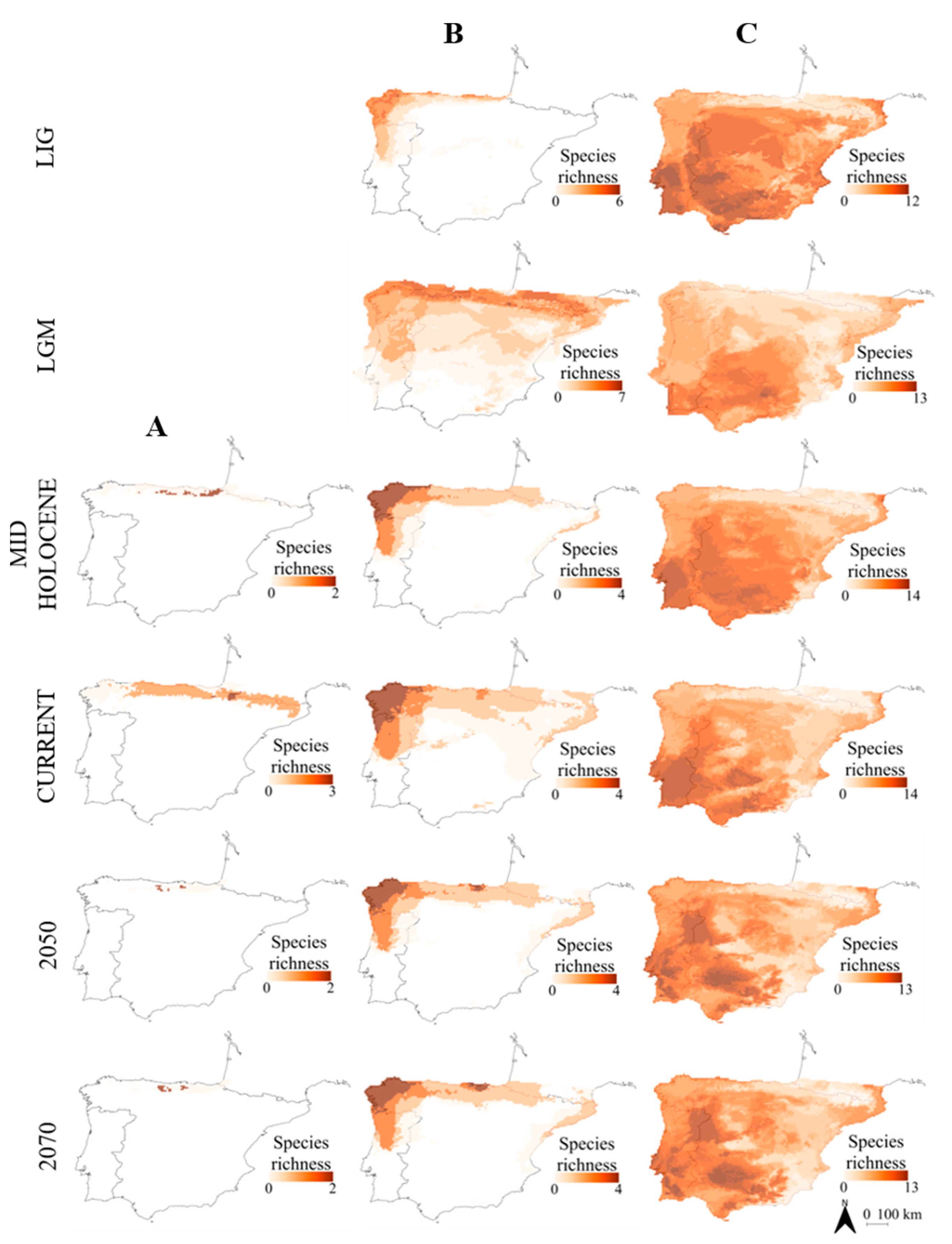
Atlantic amphibians included species with northern distribution (chorotype B; Figure 2) and cold-adapted species with their range restricted to Pyrenean-Cantabrian mountains (chorotype A; Figure 2). This pattern agrees with the mentioned previous studies, with some exceptions: for instance, Alytes obstetricans was placed in an Atlantic chorotype (chorotype B; Figure 2), when it was previously considered as mainly Mediterranean [10,90]. However, this species is distributed in central Europe, although it has a high percentage of occurrence in both Iberian regions [10].

-

Mediterranean amphibians (chorotype C; Figure 2) included several generalists and wide range species (such as Pleurodeles waltl), corresponding mostly to the Western and Iberian chorotypes considered by Vargas and Real [90].

-

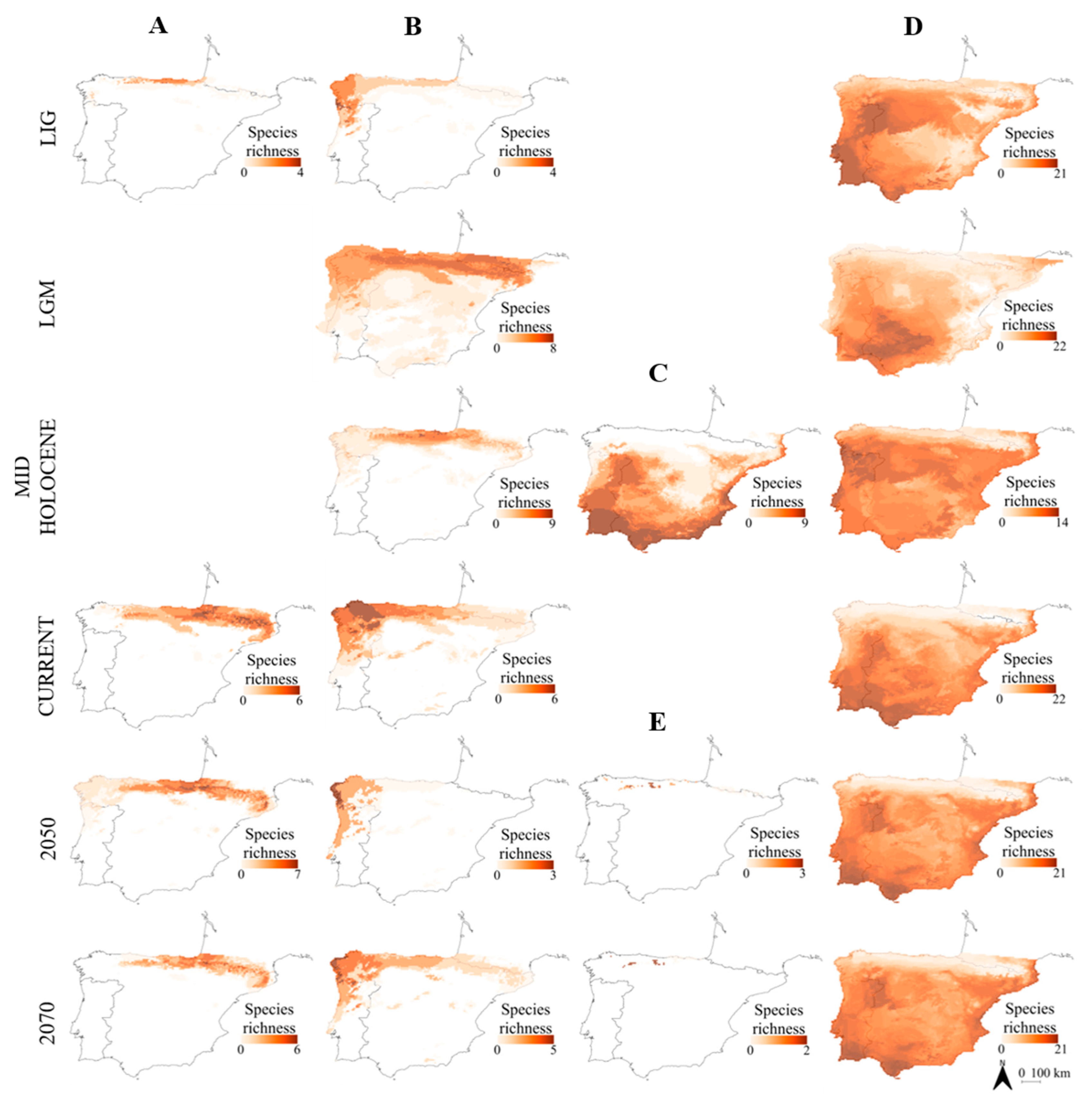
Atlantic reptiles included species with northern distribution (chorotype B; Figure 3), species with their range restricted to the Pyrenean-Cantabrian mountains (chorotype A; Figure 3) and species with their range limited to the Cantabrian region (chorotype E; Figure 3). Some species fluctuated between different chorotypes depending on the temporal period. For instance, Lacerta schreiberi was placed in a Mediterranean chorotype in the three scenarios of the past (LIG, LGM and Mid Holocene; chorotype D; Figure 3), but in an Atlantic chorotype in the present and future scenarios (chorotype B; Figure 3). This species was previously associated with Atlantic climates [10], but it does occupy riverine habitats; thus, it can persist in Mediterranean habitats [65].

-

Mediterranean reptiles included one chorotype with all the widespread species in most periods (chorotype D; Figure 3), except for the Mid Holocene that included two chorotypes, with a species composition very similar to the one obtained by Sillero et al. [10]: the chorotype C (Figure 3) includes species that commonly avoid the eastern and northern part of the peninsula and also species occurring in North Africa (such as Hemorrhois hippocrepis); the chorotype D (Figure 3) includes species with Palearctic distributions, species present in both Africa and in southern France.

Overall, the hotspots for amphibians and reptiles in the Atlantic region were located in the north-west of the Iberian Peninsula and in the Pyrenees-Cantabrian region (Figure 2 and Figure 3), as obtained by Sillero et al. [10]. The last glacial period (LGM) had a noticeable greater species richness, while in warmer periods (e.g., LIG or Mid Holocene) the richness decreases. The hotspots for amphibians and reptiles in the Mediterranean region were generally located in the south-west of the Iberian Peninsula. In the LGM, these hotspots were less significant and more balanced with the richness of the Atlantic region. In an expected warmer future, the species richness of amphibians in the Mediterranean region will become more fragmented, while reptiles will suffer fewer changes. In the case of reptiles, the Mediterranean coast (south-east of the peninsula) had also great species richness over time, but not for amphibians, this was probably due to the great aridity in this region [91].

The increase of suitable habitats for many amphibians and reptiles during past colder periods (LGM; Figure 2, Figure 3 and Figure 4) confirms the Iberian Peninsula as an important refugium for European species during glaciations [54,55], and consequently a source of endemism [10,30,92]. Most of the Iberian species with expanding ranges during glacial periods (e.g., during the LGM) are expected to contract their ranges in a future warming scenario (Figure 4) [30,93,94]. There are some exceptions, probably due to the inclusion of species together (e.g., Triturus marmoratus/pygmaeus). We found that 64% of the amphibians and reptiles will contract their range until 2070 (14 amphibians and 21 reptiles), and 36% of the amphibians and reptiles will expand their range in the future (seven amphibians and 13 reptiles). In our models, some species contracted their range in 2050 but expanded in 2070, or the contrary. Only three amphibians and seven reptiles consistently contracted their range (i.e., decreased their range area from the present to 2050, and from 2050 to 2070) and only three amphibians and six reptiles expanded their range consistently. It seems that climate change predictions have worsened during the period between the 4th and 5th IPCC reports [70,71]. Nevertheless, our results are not so different from the ones obtained by Carvalho et al. [40], who predicted that 46% of the amphibians and reptiles of the Iberian Peninsula will consistently reduce their distribution until 2080 (nine amphibians, eight reptiles) and 28% of the species will increase their distribution (three amphibians, eight reptiles). Moreover, caution must be taken when interpreting models extrapolated to conditions never encountered before, due to large uncertainty in climate change scenarios [95].

All species with restricted ranges in the present (amphibians, Alytes dickhilleni, Calotriton asper, Chioglossa lusitanica, Ichthyosaura alpestris; and reptiles, Chamaeleo chamaeleon, Hierophis viridiflavus, Iberolacerta monticola, Podarcis bocagei, Podarcis carbonelli, Zamenis longissimus/lineatus, Zooteca vivipara) will reduce their suitable range in the future, especially amphibians. These species may not be able to compensate their ranges elsewhere, significantly reducing their distributions; this identifies their vulnerability to climate change [40]. This is particularly problematic for cold-adapted range-restricted species, such as Calotriton asper (expected to contract their range from 51,300 km² in the present to 20,200 km² in 2070), Ichthyosaura alpestris (range contraction of 41,300 km² to 3000 km²) or Iberolacerta monticola (range contraction of 56,800 km² to 2500 km²), because colder climates are disappearing [89,96]. These species will not have room to disperse in response to future global warming [29]. Araújo et al. [94] suggested that the contemporary climate affects more widespread species, while the past climates affected more the narrow-ranged ones. However, we did not observe this pattern: from the 45 widespread species analysed, we predicted that 26 will contract their range until 2070.

Climate factors (such as temperature and precipitation) are strongly correlated to species biogeographical patterns [10,30]. The Iberian Peninsula has a south-east/north-west precipitation gradient during rainy months and a south/north precipitation gradient during drier and warmer months [91,97]. The refugia areas for amphibians are the most humid regions of the peninsula, and the less important areas (eastern part of the peninsula; Figure 5) correspond to most arid areas, especially during the rainy season [91]. Therefore, these important areas have higher levels of precipitation throughout the year. Reptiles are not as dependent on water availability as amphibians [59], and their refugia areas are located mostly in the southern part of the peninsula and on the Atlantic coast. Interestingly, the northern part of the peninsula (also the colder region; [91]) seems to be the least important for reptiles over time. This could represent a limiting factor in the distribution of reptiles in the north. However, Moreno-Rueda et al. [44] predicted a northward shift of reptiles with climate change in Spain. Thus, this pattern of reptiles’ refugia areas may change in the future.

Assessing the vulnerability of species chorotypes to climate change is critical for effective conservation efforts [98]. Some areas are more important for species persistence than others, constituting important refugia in the light of the environmental changes of the past and future. The Mediterranean Basin, and the Iberian Peninsula, in particular, are one of the most vulnerable areas to climate change, due to the predicted increase of aridity and drought risk [29,35,36,40,99,100]. To our knowledge, this is the first attempt to analyse changes in biogeographic regions of amphibians and reptiles over time. Our predictions could be improved by performing the analysis with data at higher spatial resolution. Further research should include an analysis of the altitudinal shifts of amphibians and reptiles in the Iberian Peninsula, as well as the introduction of historical processes (such as speciation events), ecological variables (such as competition and predation) and human-induced variables (such as road mortality and habitat fragmentation) [10]. The identification of species biogeographical patterns and important areas of refugia over time in the light of past climate changes are essential to apply conservation measures and to target the research on these sites, which include the monitoring of species, mitigation of important threats and increase species potential of dispersal (e.g., restoring habitats, increasing connectivity between suitable habitats or assisting species colonization [40,101]). However, these actions will not be enough if the human population continues to increase uncontrolled [102].

References

1. Pettorelli, N.; Laurance, W.F.; O’Brien, T.G.; Wegmann, M.; Nagendra, H.; Turner, W. Satellite remote sensing for applied ecologists: Opportunities and challenges. J. Appl. Ecol. 2014, 51, 839–848. [Google Scholar] [CrossRef]
2. He, K.S.; Bradley, B.A.; Cord, A.F.; Rocchini, D.; Tuanmu, M.N.; Schmidtlein, S.; Turner, W.; Wegmann, M.; Pettorelli, N. Will remote sensing shape the next generation of species distribution models? Remote Sens. Ecol. Conserv. 2015, 1, 4–18. [Google Scholar] [CrossRef] [Green Version]
3. Leitão, P.J.; Santos, M.J. Improving models of species ecological niches: A remote sensing overview. Front. Ecol. Evol. 2018, 7, 9. [Google Scholar] [CrossRef] [Green Version]
4. Pasetto, D.; Arenas-Castro, S.; Bustamante, J.; Casagrandi, R.; Chrysoulakis, N.; Cord, A.F.; Dittrich, A.; Domingo-Marimon, C.; Serafy, E.; Karnieli, A. Integration of satellite remote sensing data in ecosystem modelling at local scales: Practices and trends. Methods Ecol. Evol. 2018, 9, 1810–1821. [Google Scholar] [CrossRef] [Green Version]
5. Sillero, N.; Vale, C.G.; Beukema, W. GIS for spatial biology: The geographical component of life. Front. Inf. Syst. 2018, 1, 149–183. [Google Scholar] [CrossRef]
6. Vargas, J.M.; Real, R.; Guerrero, J.C. Biogeographical regions of the Iberian Peninsula based on freshwater fish and amphibian distributions. Ecography 1998, 21, 371–382. [Google Scholar] [CrossRef]
7. Lenormand, M.; Papuga, G.; Argagnon, O. Biogeographical network analysis of plant species distribution in the Mediterranean region. Ecol. Evol. 2018, 9, 237–250. [Google Scholar] [CrossRef]
8. Baroni-Urbani, C.; Ruffo, S.; Taglianti, V. Materiali per uma biogeografia italiana fondata se alcuni generi di coleotteri Cicindelidi, Carabidi, e Crisomelidi. Mem. Soc. Entomol. Ital. 1978, 56, 35–92. [Google Scholar]
9. Passalacqua, N.G. On the definition of element, chorotype and component in biogeography. J. Biogeogr. 2015, 42, 611–618. [Google Scholar] [CrossRef]
10. Sillero, N.; Brito, J.C.; Skidmore, A.K.; Toxopeus, A.G. Biogeographical patterns derived from remote sensing variables: The amphibians and reptiles of the Iberian Peninsula. Amphib. Reptil. 2009, 30, 185–206. [Google Scholar] [CrossRef]
11. Humboldt, A. Essai sur la Geographie des Plantes; Accompagne d'un Tableau Physique des Régions Equinoxiales; Levrault, Schoell et Compagnie: Paris, France, 1805. [Google Scholar]
12. Sclater, P. On the geographical distribution of the members of the class Aves. J. Linn. Soc. Zool. 1858, 2, 130–145. [Google Scholar] [CrossRef]
13. Wallace, A.R. The Geographical Distribution of Animals; Macmillan: London, UK, 1876. [Google Scholar]
14. Vilhena, D.A.; Antonelli, A. A network approach for identifying and delimiting biogeographical regions. Nat. Commun. 2015, 6, 6848. [Google Scholar] [CrossRef] [PubMed]
15. Holt, B.G.; Lessard, J.-P.; Borregaard, M.K.; Fritz, S.A.; Araújo, M.B.; Dimitrov, D.; Fabre, P.H.; Graham, C.H.; Graves, G.R.; Jønsoon, K.A. An update of Wallace’s zoogeographic regions of the world. Science 2013, 339, 74–78. [Google Scholar] [CrossRef] [Green Version]
16. Kreft, H.; Jetz, W. A framework for delineating biogeographical regions based on species distributions. J. Biogeogr. 2010, 37, 2029–2053. [Google Scholar] [CrossRef]
17. Chapin, J.P. Ecological aspects of bird distribution in tropical Africa. Am. Nat. 1923, 57, 106–125. [Google Scholar] [CrossRef]
18. Simpson, G.G. Too many lines: The limits of the Oriental and Australian zoogeographic regions. Proc. Am. Philos. Soc. 1977, 121, 107–120. [Google Scholar]
19. Crowe, T.M.; Crowe, A.A. Patterns of distribution, diversity and endemism in Afrotropical birds. J. Zool. 1982, 198, 417–442. [Google Scholar] [CrossRef]
20. Smith, S.A.; Bermingham, E. The biogeography of lower Mesoamerican freshwater fishes. J. Biogeogr. 2005, 32, 1835–1854. [Google Scholar] [CrossRef]
21. Sillero, N.; Campos, J.C.; Bonardi, A.; Corti, C.; Creemers, R.; Crochet, P.A.; Crnobrnja-Isailovic, J.; Denoel, M.; Ficetola, G.F.; Gonçalves, J. Updated distribution and biogeography of amphibians and reptiles of Europe. Amphib. Reptil. 2014, 35, 1–31. [Google Scholar] [CrossRef] [Green Version]
22. Moreno Saiz, J.C.; Donato, M.; Katinas, L.; Crisci, J.V.; Posadas, P. New insights into the biogeography of south-western Europe: Spatial patterns from vascular plants using cluster analysis and parsimony. J. Biogeogr. 2013, 40, 90–104. [Google Scholar] [CrossRef]
23. Freitas, R.; Romeiras, M.; Silva, L.; Cordeiro, R.; Madeira, P.; González, J.A.; Wirtz, P.; Falcón, J.M.; Brito, A.; Floeter, S.R. Restructuring of the ‘Macaronesia’ biogeographic unit: A marine multi-taxon biogeographical approach. Sci. Rep. 2019, 9, 15792. [Google Scholar] [CrossRef] [PubMed] [Green Version]
24. López, H.L.; Menni, R.C.; Donato, M.; Miquelarena, A.M. Biogeographical revision of Argentina (Andean and Neotropical Regions): An analysis using freshwater fishes. J. Biogeogr. 2008, 35, 1564–1579. [Google Scholar] [CrossRef] [Green Version]
25. Peterson, A.T. Ecological niche conservatism: A time-structured review of evidence. J. Biogeogr. 2011, 38, 817–827. [Google Scholar] [CrossRef]
26. Jarnevich, C.S.; Stohlgren, T.J.; Kumar, S. Caveats for correlative species distribution modelling. Ecol. Inf. 2015, 29, 6–15. [Google Scholar] [CrossRef]
27. Guisan, A.; Zimmermann, N.E. Predictive habitat distribution models in ecology. Ecol. Model. 2000, 135, 147–186. [Google Scholar] [CrossRef]
28. Feng, X.; Park, D.S.; Walker, C.; Peterson, A.T.; Merow, C.; Papes, M. A checklist for maximizing reproducibility of ecological niche models. Nat. Ecol. Evol. 2019, 3, 1382–1395. [Google Scholar] [CrossRef] [Green Version]
29. Araújo, M.B.; Thuiller, W.; Pearson, R.G. Climate warming and the decline of amphibians and reptiles in Europe. J. Biogeogr. 2006, 33, 1712–1728. [Google Scholar] [CrossRef]
30. Sillero, N.; Carretero, M.A. Modelling the past and future distribution of contracting species. The Iberian lizard Podarcis carbonelli (Squamata: Lacertidae) as a case study. Zool. Anz. 2013, 252, 289–298. [Google Scholar] [CrossRef]
31. Peterson, A.T.; Pape, M.; Eaton, M. Transferability and model evaluation in ecological niche modeling: A comparison of GARP and Maxent. Ecography 2007, 30, 550–560. [Google Scholar] [CrossRef]
32. Nogués-Bravo, D. Predicting the past distribution of species climatic niches. Glob. Ecol. Biogeogr. 2009, 18, 521–531. [Google Scholar] [CrossRef]
33. Franklin, J. Moving beyond static species distribution models in support of conservation biogeography. Divers. Distrib. 2010, 16, 321–330. [Google Scholar] [CrossRef]
34. Seabra, R.; Wethey, D.; Santos, A.M.; Lima, F.P. Understanding complex biogeographic responses to climate change. Sci. Rep. 2015, 5, 12930. [Google Scholar] [CrossRef] [PubMed]
35. Giorgi, F. Climate changes hot-spots. Geophys. Res. Lett. 2006, 33, L08707. [Google Scholar] [CrossRef]
36. Vicente-Serrano, S.M.; Lopez-Moreno, J.-I.; Beguería, S.; Lorenzo-Lacruz, J.; Sanchez-Lorenzo, A.; García-Ruiz, J.M.; Azorin-Molina, C.; Morán-Tejeda, E.; Revuelto, J.; Trigo, R. Evidence of increasing drought severity caused by temperature rise in southern Europe. Environ. Res. Lett. 2014, 9, 044001. [Google Scholar] [CrossRef]
37. Thiébault, S.; Moatti, J.-P. (Eds.) The Mediterranean Region under Climate Change: A Scientific Update; IRD: Marseille, France, 2016; p. 133. [Google Scholar]
38. Knapp, A.K.; Smith, M.D. Variation among biomes in temporal dynamics of aboveground primary production. Science 2001, 291, 481–484. [Google Scholar] [CrossRef] [Green Version]
39. Salazar, L.F.; Nobre, C.A.; Oyama, M.D. Climate change consequences on the biome distribution in tropical South America. Geophys. Res. Lett. 2007, 34, L09708. [Google Scholar] [CrossRef] [Green Version]
40. Carvalho, S.B.; Brito, J.C.; Crespo, E.J.; Possingham, H.P. From climate change predictions to actions—Conserving vulnerable animal groups in hotspots at a regional scale. Glob. Chang. Biol. 2010, 16, 3257–3270. [Google Scholar] [CrossRef]
41. Rebelo, H.; Tarroso, P.; Jones, G. Predicted impact of climate change on European bats in relation to their biogeographic patterns. Glob. Chang. Biol. 2010, 16, 561–576. [Google Scholar] [CrossRef]
42. Serra-Diaz, J.M.; Franklin, J. What’s hot in conservation biogeography in a changing climate? Going beyond species range dynamics. Divers. Distrib. 2019, 25, 492–498. [Google Scholar] [CrossRef] [Green Version]
43. Chen, I.C.; Hill, J.K.; Ohlemuller, R.; Roy, D.B.; Thomas, C.D. Rapid range shifts of species associated with high levels of climate warming. Science 2011, 333, 1024–1026. [Google Scholar] [CrossRef]
44. Moreno-Rueda, G.; Pleguezuelos, J.M.; Pizarro, M.; Montori, A. Northward shifts of the distributions of Spanish reptiles in association with climate change. Conserv. Biol. 2011, 26, 278–283. [Google Scholar] [CrossRef] [PubMed]
45. Auer, S.K.; King, D.I. Ecological and life-history traits explain recent boundary shifts in elevation and latitude of western North American songbirds. Glob. Ecol. Biogeogr. 2014, 23, 867–875. [Google Scholar] [CrossRef]
46. Williams, J.E.; Blois, J.L. Range shift in response to past and future climate change: Can climate velocities and species’ dispersal capabilities explain variation in mammalian range shifts? J. Biogeogr. 2018, 45, 2175–2189. [Google Scholar] [CrossRef]
47. Borzée, A.; Andersen, D.; Groffen, J.; Kim, H.T.; Bae, Y.; Jang, Y. Climate change-based models predict range shifts in the distribution of the only Asian plethodontid salamander: Karsenia koreana. Sci. Rep. 2019, 9, 11838. [Google Scholar] [CrossRef] [PubMed] [Green Version]
48. Rosalino, L.M.; Guedes, D.; Cabecinha, D.; Serronha, A.; Grilo, C.; Santos-Reis, M.; Monterroso, P.; Carvalho, J.; Fonseca, C.; Pardavila, X. Climate and landscape changes as driving forces for future range shift in southern populations of the European badger. Sci. Rep. 2019, 9, 3155. [Google Scholar] [CrossRef] [PubMed] [Green Version]
49. Myers, N.; Mittermeier, R.A.; Mittermeier, C.G.; Fonseca, G.A.B.; Kent, J. Biodiversity hotspots for conservation priorities. Nature 2000, 6772, 853–858. [Google Scholar] [CrossRef]
50. Pascual, L.L.; Luigi, M.; Alessandra, F.; Emilio, B.; Luigi, B. Hotsposts of species richness, threat and endemism for terrestrial vertebrates in SW Europe. Acta Oecol. 2011, 37, 399–412. [Google Scholar] [CrossRef]
51. Sillero, N. What does ecological modelling model? A proposed classification of ecological niche models based on their underlying methods. Ecol. Model. 2011, 222, 1343–1346. [Google Scholar] [CrossRef]
52. Álvarez-López, E.A. Los caracteres geográficos de la herpetofauna ibérica (Contribución al estudio de la Zoogeografía peninsular). Bol. Real Soc. Hist. Nat. (Secc. Biol.) 1934, 34, 327–374. [Google Scholar]
53. Williams, P.H.; Humphries, C.; Araújo, M.B.; Lampinen, R.; Hagemeijer, W.; Gasc, J.P.; Mitchell-Jones, T. Endemism and important areas for representing European biodiversity: A preliminary exploration of atlas data for plants and terrestrial vertebrates. Belg. J. Entomol. 2000, 2, 21–46. [Google Scholar]
54. Hewitt, G.M. Some genetic consequences of ice ages, and their role in divergence and speciation. Biol. J. Linn. Soc. 1996, 58, 247–276. [Google Scholar] [CrossRef]
55. Hewitt, G.M. The genetic legacy of the Quaternary ice ages. Nature 2000, 22, 907–913. [Google Scholar] [CrossRef] [PubMed]
56. Rivas-Martínez, S. Mapa de Series, Geoseries y Geopermaseries de Vegetación de España, Parte 1. Memoria del Mapa de Vegetación Potencial de España; Universidad Complutense: Madrid, Spain, 2005; pp. 1–28. [Google Scholar]
57. European Environment Agency. Biogeographical Regions; European Environment Agency: Copenhagen, Denmark, 2016. [Google Scholar]
58. Blondel, J.; Aronson, J. Biology and Wildlife of the Mediterranean Region; Oxford University Press: Oxford, UK, 1999; p. 352. [Google Scholar]
59. Gibbons, J.W.; Scott, D.E.; Ryan, T.J.; Buhlmann, K.A.; Tuberville, T.D.; Metts, B.S.; Greene, J.L.; Mills, T.; Leiden, Y.; Poppy, S.; et al. The global decline of reptiles, déjà vu amphibians. BioScience 2000, 50, 653–661. [Google Scholar] [CrossRef] [Green Version]
60. Houlahan, J.E.; Findlay, C.S.; Schmidt, B.R.; Meyer, A.H.; Kuzmin, S.L. Quantitative evidence for global amphibian population declines. Nature 2000, 404, 752–755. [Google Scholar] [CrossRef]
61. Aragón, P.; Rodríguez, M.A.; Olalla-Tárraga, M.A.; Lobo, J.M. Predicted impact of climate change on threatened terrestrial vertebrates in central Spain highlights differences between endotherms and ectotherms. Anim. Conserv. 2010, 13, 363–373. [Google Scholar] [CrossRef]
62. Stuart, S.N.; Chanson, J.S.; Cox, N.; Young, B.E.; Rodrigues, A.S.L.; Fischman, D.L.; Waller, R.W. Status and trends of amphibian declines and extinctions worldwide. Science 2004, 306, 1783–1786. [Google Scholar] [CrossRef] [Green Version]
63. Böhm, M.; Collen, B.; Baillie, J.E.M.; Bowles, P.; Chanson, J.; Cox, N.; Hammerson, G.; Hoffmann, M.; Livingstone, S.R.; Ram, M. The conservation status of the world’s reptiles. Biol. Conserv. 2013, 157, 372–385. [Google Scholar] [CrossRef]
64. Pleguezuelos, J.M.; Márquez, R.; Lizana, M. Atlas de distribución y Libro Rojo de los Anfibios y Reptiles de España; Dirección General de Conservación de la Naturaleza-Asociación Herpetológica Española: Madrid, Spain, 2002. [Google Scholar]
65. Loureiro, A.; Ferrand de Almeida, N.; Carretero, M.A.; Paulo, O.S. (Eds.) Atlas dos Anfíbios e Répteis de Portugal, 1st ed.; Instituto de Conservação da Natureza e da Biodiversidade: Lisbon, Portugal, 2010; p. 257. [Google Scholar]
66. Comisión de Taxonomía de la AHE. Lista Patrón de los Anfibios y Reptiles de España: Conclusiones de Nomenclatura y Taxonomía para las Especies de Anfibios y Reptiles de España; Asociación Herpetológica Española: Barcelona, Spain, 2018. [Google Scholar]
67. Hijmans, R.J.; Cameron, S.E.; Parra, J.L.; Jones, P.G.; Jarvis, A. Very high resolution interpolated climate surfaces for global land areas. Int. J. Climatol. 2005, 25, 1965–1978. [Google Scholar] [CrossRef]
68. Bedia, J.; Herrera, S.; Gutiérrez, J.M. Dangers of using global bioclimatic datasets for ecological niche modeling. Limitations for future climate projections. Glob. Planet. Chang. 2013, 107, 1–12. [Google Scholar] [CrossRef] [Green Version]
69. Varela, S.; Lima-Ribeiro, M.S.; Terribile, L.C. A short guide to the climatic variables of the Last Glacial Maximum for biogeographers. PLoS ONE 2015, 10, e0129037. [Google Scholar] [CrossRef]
70. IPCC. Climate Change 2007: Synthesis Report. Contribution of Working Groups I, II and III to the Fourth Assessment Report of the Intergovernmental Panel on Climate Change; Core Writing Team, Pachauri, R.K., Reisinger, A., Eds.; IPCC: Geneva, Switzerland, 2007; p. 104. [Google Scholar]
71. IPCC. Climate Change 2014: Synthesis Report. Contribution of Working Groups I, II and III to the Fifth Assessment Report of the Intergovernmental Panel on Climate Change; Core Writing Team, Pachauri, R.K., Meyer, L.A., Eds.; IPCC: Geneva, Switzerland, 2014; p. 151. [Google Scholar]
72. Otto-Bliesner, B.L.; Marshall, S.J.; Overpeck, J.T. Simulating Arctic climate warmth and icefield retreat in the last interglaciation. Science 2006, 311, 1751–1753. [Google Scholar] [CrossRef] [PubMed] [Green Version]
73. MacDougall, J.D. A Short History of Planet Earth: Mountains, Mammals, Fire and Ice; John Wiley & Sons, Inc.: New York, NY, USA, 1996; p. 274. [Google Scholar]
74. Clark, P.U.; Dyke, A.S.; Shakun, J.D.; Carlson, A.E.; Clark, J.; Wohlfarth, B.; Mitrovica, J.X.; Hostetler, S.W.; McCabe, M. The last glacial maximum. Science 2009, 325, 710–714. [Google Scholar] [CrossRef] [PubMed] [Green Version]
75. McSweeney, C.F.; Jones, R.G.; Lee, R.W.; Rowell, D.P. Selecting CMIP5 GCMs for downscaling over multiple regions. Clim. Dyn. 2015, 44, 3237–3260. [Google Scholar] [CrossRef] [Green Version]
76. Phillips, S.J.; Anderson, R.P.; Schapire, R.E. Maximum entropy modelling of species geographic distributions. Ecol. Model. 2006, 190, 231–259. [Google Scholar] [CrossRef] [Green Version]
77. Phillips, S.J.; Dudik, M. Modeling of species distributions with Maxent: New extensions and a comprehensive evaluation. Ecography 2008, 31, 161–175. [Google Scholar] [CrossRef]
78. Guillera-Arroita, G.; Lahoz-Monfort, J.J.; Elith, J. Maxent is not a presence-absence method: A comment on Thibaud et al. Methods Ecol. Evol. 2014, 5, 1192–1197. [Google Scholar] [CrossRef]
79. Phillips, S.J.; Anderson, R.P.; Dudík, M.; Schapire, R.E.; Blair, M.E. Opening the black box: An open-source release of Maxent. Ecography 2017, 40, 887–893. [Google Scholar] [CrossRef]
80. Phillips, S.J.; Dudík, M.; Elith, J.; Graham, C.H.; Lehmann, A.; Leathwick, J.; Ferrier, S. Sample selection bias and presence-only distribution models: Implications for background and pseudo-absence data. Ecol. Appl. 2009, 19, 181–197. [Google Scholar] [CrossRef] [Green Version]
81. Liu, C.; Berry, P.M.; Dawson, T.P.; Pearson, R.G. Selecting thresholds of occurrence in the prediction of species distributions. Ecography 2005, 28, 385–393. [Google Scholar] [CrossRef]
82. Raes, N.; ter Steege, H. A null-model for significance testing of presence-only species distribution models. Ecography 2007, 30, 727–736. [Google Scholar] [CrossRef]
83. R Core Team. R: A Language and Environment for Statistical Computing; R Foundation for Statistical Computing: Vienna, Austria, 2011. [Google Scholar]
84. Hijmans, R.J.; Phillips, S.; Leathwick, J.; Elith, J. Dismo: Species Distribution Modeling. R Package Version 1.1-4. 2017. Available online: http://rspatial.org/sdm/ (accessed on 12 March 2020).
85. Mac Nally, R.; Fleishman, E.; Bulluck, L.P.; Betrus, C.J. Comparative influence of spatial scale on beta diversity within regional assemblages of birds and butterflies. J. Biogeogr. 2004, 31, 917–929. [Google Scholar] [CrossRef]
86. Smith, K.G. Patterns of nonindigenous herpetofaunal richness and biotic homogenization among Florida counties. Biol. Conserv. 2006, 127, 327–335. [Google Scholar] [CrossRef]
87. Garcia, R.A.; Cabeza, M.; Rahbek, C.; Araújo, M.B. Multiple dimensions of climate change and their implications for biodiversity. Science 2014, 344, 486. [Google Scholar] [CrossRef] [PubMed] [Green Version]
88. Pacifici, M.; Foden, W.; Visconti, P.; Watson, J.E.M.; Butchart, S.H.M.; Kovacs, K.M.; Scheffers, B.R.; Hole, D.G.; Martin, T.G.; Akçakaya, R. Assessing species vulnerability to climate change. Nat. Clim. Chang. 2015, 5, 215–224. [Google Scholar] [CrossRef]
89. Enriquez-Urzelai, U.; Bernardo, N.; Moreno-Rueda, G.; Montori, A.; Llorente, G. Are amphibians tracking their climatic niches in response to climate warming? A test with Iberian amphibians. Clim. Chang. 2019, 154, 289–301. [Google Scholar] [CrossRef]
90. Vargas, J.M.; Real, R. Biogeografía de los anfibios y reptiles de la Península Ibérica. In Distribución y Biogeografía de los Anfibios y Reptiles en España y Portugal, Monografías de Herpetología; Pleguezuelos, J.M., Ed.; Asociación Herpetológica Española y Universidad de Granada: Granada, Spain, 1997; pp. 310–320. [Google Scholar]
91. Couto, M.A.; Sánchez, G.; Tavares, C.D.; Barceló, A.M.; Nunes, L.F.; Herráez, C.F.; Pires, V.; Marques, J.; Mendes, L.; Chazarra, A. Atlas Climático Ibérico; Instituto de Meteorologia de Portugal and Agencia Estatal de Meteorología, Ministerio de Medio Ambiente y Medio Rural y Marino: Madrid, Spain, 2011; p. 80. [Google Scholar]
92. Hewitt, G.M. Ice ages: Their impact on species distributions and evolution. In Evolution on Planet Earth; Rothschild, L.J., Lister, A.M., Eds.; Academic Press: New York, NY, USA, 2003; pp. 339–361. [Google Scholar]
93. Araújo, M.B.; Whittaker, R.J.; Ladle, R.J.; Erhard, M. Reducing uncertainty in projections of extinction risk from climate change. Glob. Ecol. Biogeogr. 2005, 14, 529–538. [Google Scholar] [CrossRef]
94. Araújo, M.B.; Nogués-Bravo, D.; Diniz Filho, J.A.; Haywood, A.M.; Valdes, P.J.; Rahbek, C. Quaternary climate changes explain diversity among reptiles and amphibians. Ecography 2008, 31, 8–15. [Google Scholar] [CrossRef] [Green Version]
95. Dormann, C.F. Promising the future? Global change projections of species distributions. Basic Appl. Ecol. 2007, 8, 387–397. [Google Scholar] [CrossRef]
96. Ortega, Z.; Mencía, A.; Pérez-Mellado, V. Behavioral buffering of global warming in a cold-adapted lizard. Ecol. Evol. 2016, 6, 4582–4590. [Google Scholar] [CrossRef] [Green Version]
97. Paniagua, L.L.; García-Martín, A.; Moral, F.J.; Rebollo, F.J. Aridity in the Iberian Peninsula (1960–2017): Distribution, tendencies, and changes. Theor. Appl. Climatol. 2019, 138, 811. [Google Scholar] [CrossRef]
98. Whittaker, R.J.; Araújo, M.B.; Jepson, P.; Ladle, R.; Watson, J.E.M.; Willis, K.J. Conservation Biogeography: Assessment and prospect. Divers. Distrib. 2005, 11, 3–23. [Google Scholar] [CrossRef]
99. Gao, X.; Giorgi, F. Increased aridity in the Mediterranean region under greenhouse gas forcing estimated from high resolution simulations with a regional climate model. Glob. Planet. Chang. 2008, 62, 195–209. [Google Scholar] [CrossRef]
100. Sánchez, E.; Domínguez, M.; Romera, R.; López de la Franca, N.; Gaertner, M.A.; Gallardo, C.; Castro, M. Regional modeling of dry spells over the Iberian Peninsula for present climate and climate change conditions. Clim. Chang. 2011, 107, 625–634. [Google Scholar] [CrossRef]
101. Hoegh-Guldberg, O.; Hughes, L.; McIntyre, S.; Lindenmayer, D.B.; Parmesan, C.; Possingham, H.P.; Thomas, C.D. Assisted colonization and rapid climate change. Science 2008, 321, 345–346. [Google Scholar] [CrossRef] [PubMed]
102. Maurer, B.A. Relating human population growth to the loss of biodiversity. Biodivers. Lett. 1996, 1, 1–15. [Google Scholar] [CrossRef]
Figure 1. Location of the Iberian Peninsula.
Climate 08 00042 g001
Figure 2. Changes in the Iberian amphibians’ chorotypes and their species richness over time: in the past (LIG: Last Interglacial, ~120,000–140,000 years BP; LGM: Last Glacial Maximum, ~21,000 years BP; and Mid Holocene, ~5000 years BP), present and future (2050 and 2070) scenarios. (A,B) correspond to Atlantic chorotypes, while (C) corresponds to a Mediterranean chorotype. See the species composition of each chorotype in Supplementary Materials (Figures S1–S6).
Climate 08 00042 g002
Figure 3. Changes in the Iberian reptiles’ chorotypes and their species richness over time: in the past (LIG: Last Interglacial, ~120,000–140,000 years BP; LGM: Last Glacial Maximum, ~21,000 years BP; and Mid Holocene, ~5000 years BP), present and future (2050 and 2070) scenarios. (A,B,E) correspond to Atlantic chorotypes, while (C,D) correspond to Mediterranean chorotypes. See the species composition of each chorotype in Supplementary Materials (Figures S7–S12).
Climate 08 00042 g003
Figure 4. Expansions and contractions in species ranges of Iberian amphibians and reptiles in the past (LIG: Last Interglacial, ~120,000–140,000 years BP; LGM: Last Glacial Maximum, ~21,000 years BP; and Mid Hol: Mid Holocene, ~5000 years BP), present and future (2050 and 2070) scenarios. The two graphics on the left represent species that decrease their range area from the present to 2070 and the two on the right represent species that increase their range area until 2070.
Climate 08 00042 g004
Figure 5. Areas of refugia over time for amphibians and reptiles in the Iberian Peninsula. The refugia areas are the sum of all presence/absence models of the past, present and future divided by the number of species. Amphibians had refugia areas mostly in the western part of the Iberian Peninsula, while reptiles had refugia areas in the south and centre.
Climate 08 00042 g005