A Sensitivity Study of High-Resolution Climate Simulations for Greece
by
 , , , and
Nadia Politi
1,2,* ,
,
Athanasios Sfetsos
1,
Diamando Vlachogiannis
1,
Panagiotis T. Nastos
2 and
Stylianos Karozis
1 1
Environmental Research Laboratory, INRaSTES, NSCR Demokritos, 15341 Agia-Paraskevi, Greece
2
Laboratory of Climatology and Atmospheric Environment, Faculty of Geology and Geoenvironment, National and Kapodistrian University of Athens, GR 157 84 Athens, Greece
*
Author to whom correspondence should be addressed.
Climate 2020, 8(3), 44; https://0-doi-org.brum.beds.ac.uk/10.3390/cli8030044
Submission received: 7 February 2020
/
Revised: 10 March 2020
/
Accepted: 14 March 2020
/
Published: 16 March 2020
Abstract
:In the present study, the ability of the Advanced Weather Research and Forecasting numerical model (WRF-ARW) to perform climate regionalization studies in the topographically complex region of Greece, was examined in order to explore the possibility of a more reliable selection of physical schemes for the simulation of historical and future high resolution (5 km) climate model experiments to investigate the impact of climate change. This work is directly linked to a previous study investigating the performance of seven different model setups for one year, from which the need was derived for further examination of four different simulations to investigate the model sensitivity on the representation of surface variables statistics during a 5-year period. The results have been compared with observational data for maximum and minimum air temperature and daily precipitation through statistical analysis. Clear similarities were found in precipitation patterns among simulations and observations, yielding smoothly its inter-annual variability, especially during the wettest months and summer periods, with the lowest positive percentage BIAS calculated at about 19% for the selected combination of physics parameterizations (PP3). Regarding the maximum and minimum temperature, statistical analysis showed a high correlation above 0.9, and negative bias around 1−1.5 °C, and positive bias near 2 °C, respectively.
1. Introduction
It is well known that the General Circulation Models (GCMs) are the main numerical tools that can be used by climate scientists to study the physical mechanisms of climate, and how these mechanisms are modified due to the increased emissions of greenhouse gases and pollutants, and other changes of the Earth system like changes in land use, causing the observed climate changes. The GCMs are also used extensively for the simulation of future climate projections in view of global climate change for the application of mitigation and adaptation measures. According to El-Samra et al. [1] however, a number of physical mechanisms (e.g., convection, clouds and precipitation, heterogeneity of surface fluxes and planetary boundary layer (PBL) turbulence) is not accurately represented in the GCMs for the simulation of physically consistent regional and local circulations, particularly for the regions characterized by complex topographical features, due to the rather coarse spatial resolution of approximately 80 to 300 km. To overcome such obstacles, the dynamical downscaling technique has been developed using Regional Climate Models (RCMs), and applied successfully in a number of climate modeling studies so far, such as those of [2,3,4,5,6,7,8,9,10,11].
Recent research by Sorland et al. [12] on the biases of the GCMs and RCMs has indicated that RCMs can reduce systematically the biases of the driving GCMs. The impact on the climate modeling studies of the evolution of RCMs has been reported in, e.g., [13] while in [14], a review about the current development of coupled Regional Earth System Models (RESMs) is provided. Ensemble climate simulations at 0.11 degrees spatial resolution within Euro-CORDEX, e.g., [15,16,17,18,19,20], and Med-CORDEX, e.g., [21,22] initiatives have significantly contributed towards our understanding of regional climate processes and their response to climate change.
RCMs of improved representations of climate information with high spatial resolution can explicitly resolve local features of complex terrain, areas with land–sea interactions and various land cover/land use types [3,23,24,25]. Simulations of high spatial resolution can be used for climate impact assessments, as they can better resolve physical processes of regional, mesoscale and local scale circulation effects (surface fluxes, breezes, convection and heavy precipitation) [26]. In addition, such high spatial resolution simulations are imperative when the topography of the region is rather complex with mountainous features and rough coastlines, because of the improved representation of surface characteristics and their spatial variability [27].
Several studies reported an improvement in simulated climate variables through the use of high-resolution modeling, such as, rainfall amount [4,28,29,30,31] and precipitation intensity [32,33]. Olsson et al. [34] found that using a high resolution (6 km) RCM (RCA3), low-frequency sub-daily extremes were in good agreement with the values found in point observations in Sweden. A similar study for Denmark revealed that RCM simulations at higher spatial resolutions (8 km and 12 km) represent extreme precipitation events better, and future projections depend on the combination of GCM-RCM, the spatial resolution and the temporal aggregation [35]. Nevertheless, for local scales where climate is mainly controlled by large-scale external features, the increase in spatial resolution of the RCMs does not improve the simulated results [13,24].
Recent research has focused on the performance of the Advanced Weather Research and Forecasting numerical model (WRF-ARW) to reproduce climate with high spatial resolutions at several time scales, as this model allows researchers to easily choose among a large number of physical parameterizations used to represent phenomena, including microphysics, cumulus, PBL, radiation, etc. In addition, Pieri et al. [36] pointed out the importance of investigating the sensitivity of model performance when applying different spatial resolutions, as well as convective and microphysics parameterization schemes in climate change regional impact assessment studies. A number of studies refer to climate modeling over Europe [2,37,38,39] and other on country level domains [3,4,31,40], in order to demonstrate the ability of WRF to represent extreme events of temperature or precipitation, climate indicators and drought variability, moreover aiming to generally reproduce climate features spatially and temporally with improved results, due to efficiently capturing local processes over complex topography. Many of these studies were realized in the framework of CORDEX and other projects, with spatial resolution increased from 50 km to 5 km [41]. Simulations of future climate projections by applying downscaling can be performed following the evaluation of the model for historic periods, using the same set-up [1].
For the study area that focuses on Greece, studies of forecast predictability and applications with the WRF model have been carried out, with a number of different parameterization combinations. WRF has been used to perform analysis and operational and seasonal forecasting [42,43] by the group of EREL, NCSR “Demokritos” (https://forecast.ipta.demokritos.gr/). Other studies of the area of Greece have focused on WRF sensitivity to the boundary layer parameterizations for the simulation of intense precipitation and to different physical parameterizations (microphysics, boundary layer and convective schemes) [44]. Previous sensitivity research included studies for the characteristics of convective activity over Greece, predicting lightning activity investigation [45,46], studying the urban heat island over Athens [47], or the structure of PBL over the Aegean Sea. Sensitivity studies were also carried out to estimate model performance on extreme weather events over Greece [48], and model a tornado event [49].
An extensive research was assessed by Sindosi et al. [50], remarking that for the Epirus region (north-western Greece), the inclusion of the high-resolution convective parameterization scheme improved substantially the results, apart from mountainous areas, where the results were comparable with or without the use of convective schemes. Similar conclusions were adopted through the studying of forecasts of summer thunderstorms over Athens and convective parameterization [51,52].
The geomorphological complexity of Greece enhances the need of high resolution climatology studies due to: 1) the orographic chain along the central part together with the moisturized air masses coming from the central Mediterranean Sea, 2) the extended coastal zones and numerous islands, creating inhomogeneous geographical distribution of climatic variables (rainfall, temperature, etc.). The aim of this study is to establish high resolution dynamical downscaling over the complex topography of Greece. The initial work [26], which is linked to the current, included a number of simulations that investigated the sensitivity of the WRF-ARW surface outputs to different combinations of model settings and physical processes, including horizontal resolution, PBL, convective or not, microphysics schemes, and the performance of model simulations with the optimal combination through reanalysis data. In the current work, we performed 5 years of high resolution dynamical downscaling experiments, from 2000 to 2004 inclusive, with the use of the WRF model and 5 km spatial resolution. We downscale the European Centre for Medium-Range Weather Forecasts (ECMWF) Re-Analysis (ERA-Interim) data [53] to the region of Greece. The objective of this work is to validate the high resolution downscaling simulations with the use of the available observed values of minimum and maximum daily temperature and daily precipitation, in order to select among different physics parameterizations (e.g., cloud microphysics, boundary layer and cumulus), the sufficient setup to investigate the overall model’s performance over the area of interest for subsequent high resolution historic and future climate model experiments. Section 2 focuses on the description of model setup with the different physical configurations, the observational data used for the study, along with the metrics of statistical analysis for the validation. In Section 3, the results of different simulations compared to the station data through the statistical errors and diagrams are illustrated and discussed, while the final section includes the summary and conclusions about the main findings of the study.
2. Materials and Methods
2.1. Model Setup
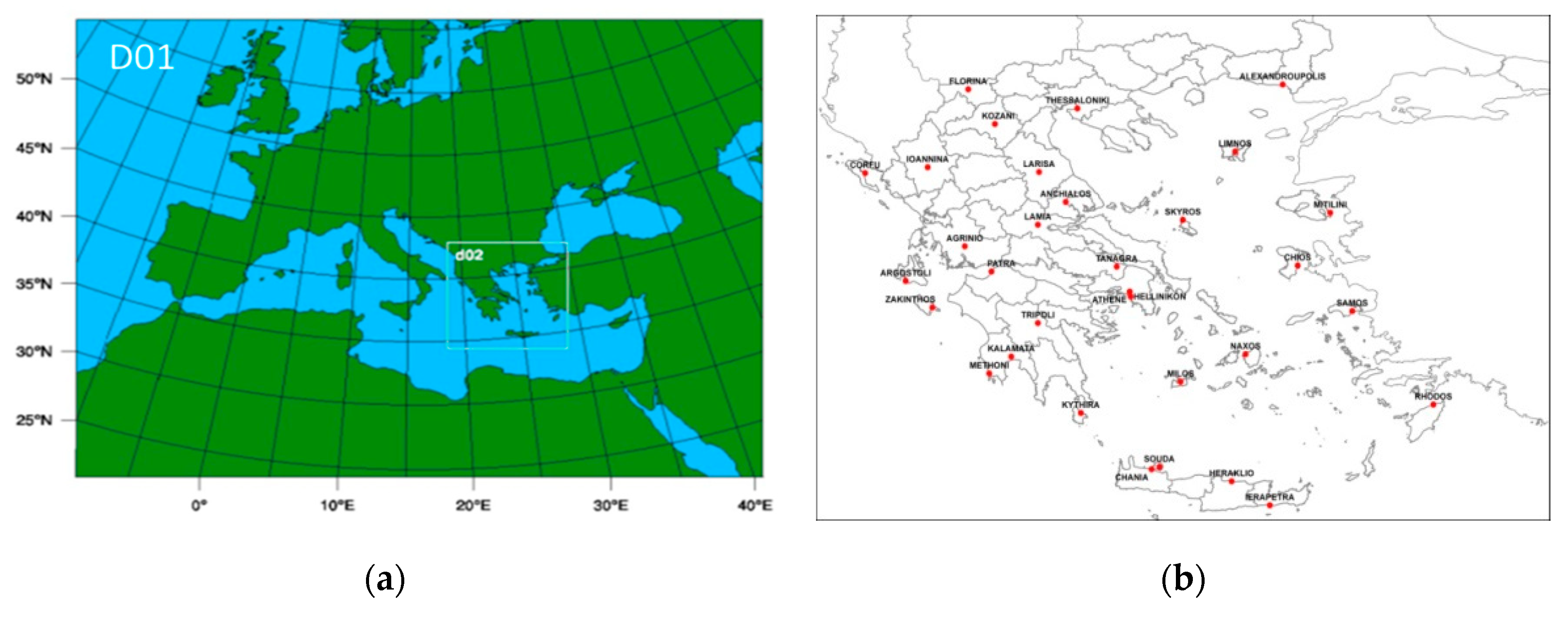
In the present study, the WRF version 3.6.1 [54] was used to perform the simulations of dynamical downscaling. WRF was setup with two nested grids (Figure 1); the outer domain, centered in the Mediterranean basin, has been configured using 265 × 200 grid cells with 20 km horizontal resolution (D01 – Europe), and the innermost domain that uses 185 x 185 grid cells of 5 km horizontal grid spacing covering the area of Greece (D02 – Greece). This setup has used 40 vertical levels arranged according to terrain-following hydrostatic pressure vertical coordinates, and one-way nesting has been applied, to avoid possible noise during feedback from the inner domain to the coarse domain. As the simulation evolves, the internal solution computed by the RCM drifts away from the driving analysis, thus spectral nudging is applied in order to reduce the effects of domain position and geometry, and to prevent any inconsistencies along boundaries over an open system [2,55,56]. The spectral nudging was applied in this study for temperature, winds and geopotential height, but not for humidity.
The period for the evaluation of all the WRF simulations spans from 1 January, 2000 until 31 December, 2004. This time period was selected based on the satisfactory number of high quality available observational data. For each simulation, the last four days of the previous month were regarded as model spin-up for the following month and were discarded, thus the model was re-initialized every month. The simulations have run independently of each other with parallel integration in order to decrease the total time needed to complete the 5-year climatology. The frequent re-initialization of the runs retains the model solution from diverging from long-term forcing, outperforms the continuous simulation runs, and distinguishes model errors that develop quickly from those over a long period [57,58,59]. In addition, similarity between modeled soil moisture suggests that monthly re-initialization does not affect the simulated surface temperature and precipitation fields. We have realized two extra experiments [60] to verify this, that have not been included in this work: with seasonal re-initialization and one continuous simulation for one year, starting December 1st of the previous year of simulation, and compared the model output to the control integration. Contingency tables and probability density function (pdf) analysis showed that the results were almost indistinguishable between the three simulations.
As already mentioned, the ERA-Interim reanalysis fields of 0.75° × 0.75° horizontal resolution were used for the initial and boundary conditions. The lateral boundary conditions and sea surface temperature were both updated every 6 hours from ERA-Interim. According to Dulière et al. [61], reanalysis data can be used for the evaluation of regional models, as they represent adequately the large-scale forcing necessary for the models to simulate the physical processes and surface interactions.
In the current study, four WRF simulations have been performed, using different combinations of physics parameterizations, in order to investigate their effects on temperature and precipitation fields in the inner domain of Greece. These different experiments were finally selected considering previous results for the same area, employing a larger set of WRF simulations covering 1-year period and more variables, such as relative humidity and surface wind speed [26]. For convenience and link to this previous research, we kept the names of the four best selected combinations of physics parameterizations (as PP2, PP3, PP5, PP7).
Table 1 summarizes the different physical schemes combinations for each of the four simulations. More specifically, two different Planetary Boundary Layer (PBL) schemes, Yonsei University (YSU); [62] and Mellor–Yamada–Janjic (MYJ); [63] were employed, associated with the corresponding surface layers (SLP) schemes, which provide the surface fluxes of momentum, moisture and heat to the PBL scheme. The MYJ scheme is a local closure model which applies a local approach to determine eddy diffusion coefficients, based on the local turbulent kinetic energy (TKE) equation. No information from lower or higher levels directly influences these terms. In this scheme, the entrainment develops only from local mixing. In contrast, the YSU scheme is a non-local closure scheme, where the critical Richardson number that describes the top of the PBL is set to 0.25 over land for enhancing mixing in the stable boundary layer. In this case, entrainment is explicitly treated.
Regarding cloud microphysics, three schemes were used in total: the WRF single-moment six-class (WSM-6) containing ice, snow and graupel processes [64], the Ferrier (FE) and the Thompson (THOM), which includes six classes of moisture for ice as prognostic variables [65]. For the cumulus parameterization, the Grell-3D (G3) [66] and Betts–Miller–Janjic (BMJ) [67] schemes were chosen, taking into consideration the gray zone between 5 and 10 km for cumulus option.
The radiation scheme was set to the newer version of the Rapid Radiative Transfer Model, RRTMG; [68] for both longwave and shortwave radiation. Only the Noah LSM was employed as the land surface model (LSM), as it is widely adopted for climate studies [69,70,71]. According to Cavan et al. [72], the scheme allows the simulation of soil and land surface temperature, snow depth and snow water equivalent, both water and energy fluxes, among others e.g. [69,73,74]. The Noah Scheme has four distinct soil layers (0.1, 0.3, 0.6 and 1.0 m) that reach a total depth of 2 m, and one vegetation canopy layer. For the estimation of potential evapotranspiration (PET), the Penman equation is used, while 16 soil and vegetation parameters are utilized for the estimation of soil temperature, soil moisture, snow cover and atmospheric feedbacks [75].
2.2. Observational Datasets
The observational data were provided by the Hellenic National Meteorological Service (HNMS) of Greece in the ECA and D project. The availability of continuous observations covering the selected period of 5 years was limited, as complete daily data existed only from a limited number of stations representing various geoclimatic regions of Greece. In total, 28 stations provided daily minimum and maximum temperatures, and 23 stations daily precipitation during the 5-year study period. It is emphasized that there is not any additional high-resolution gridded dataset covering the domain of interest. Furthermore, gridded data, such as the E-OBS dataset, are constructed with a relatively coarse network density for certain areas (including the Greek territory), with a small number of stations, implying over-smoothing across extreme percentiles of temperature and precipitation values in the resulting interpolation [76].
2.3. Analysis and Data Handling
The analysis did involve comparisons of the WRF model simulations with available measurements from the various stations of the inner (nested) domain. To evaluate the WRF downscaling results and model performance, daily maximum and minimum statistics are derived from the 6-h data simulations. Four statistical indices were estimated, the root mean square error (RMSE), which gives an overview of the accuracy of the simulations, the BIAS that indicates whether the model over- or under-predicts the given meteorological value, the mean absolute error (MAE), a measure of the absolute values of the model errors and the Pearson’s correlation coefficient (COR), a measure of linear correlation between observations and simulation data. The model error is calculated as the difference between the modeled and observed value. Further analysis of meteorological variables was done on a daily basis based on percentiles and probability density function plots.
In addition, Taylor diagrams were used to provide a comprehensive statistical and graphical assessment of how well the simulated and observed values compare with each other in terms of their correlation and normalized standard deviation, depending on the choice of the physical parameterizations [77]. Taylor diagrams and statistical metrics were calculated for seasonal and yearly time periods for the examined variables of daily maximum temperature (TX) maximum temperature (TX) and precipitation (PR). The white circle represents the standard deviation of the observational data. The formula of the calculated statistical metrics is given in Table 2:
Where is the value of the observational data, is the simulated data, and “n” is the total number of gridded locations that the model data are compared against observations.
The simulated values are taken at the center of the grid cell for temperature and precipitation. The evaluation of daily variables was made using the nearest grid point of the model to the corresponding location of the observed station, in order to find the statistical metric at that grid point [1,3,78]. The total RMSE, for example, for the Greek area, was then found by integrating the area averages (WRF model grid cell) and stations points. Because of the limited and easy to handle number of Greek stations, results are also examined and presented for each station in order to spatially evaluate the WRF model simulations skills in detail.
Height differences between model topography and stations are observed because of the complexity of the topography and the coastlines of the area. Thus, before the statistical analysis for temperature, a constant lapse-rate elevation correction of 6 °C/km had to be applied [3,23,79,80].
The accuracy of the simulated precipitation was also determined by statistical scores of a contingency table (Table 3): probability of detection (POD), critical success index (CSI) and false alarm ratio (FAR). In this study we use for four distinct threshold values of precipitation for low rainfall (>1mm), medium rainfall (>2.5 mm), heavy rainfall (>10 mm) and extremely heavy rainfall days (>20 mm) [81,82,83,84], to evaluate small and large rainfall events, for the location of each station separately.
3. Results and Discussion
In this section, the results of the WRF sensitivity experiments are presented and discussed, as emerged through the comparison with weather station datasets. The analysis is divided per daily precipitation and maximum and minimum temperatures, which are the most important for the definition of climate indices, related to future impact studies, such as heat and cold waves and drought events.
3.1. Precipitation
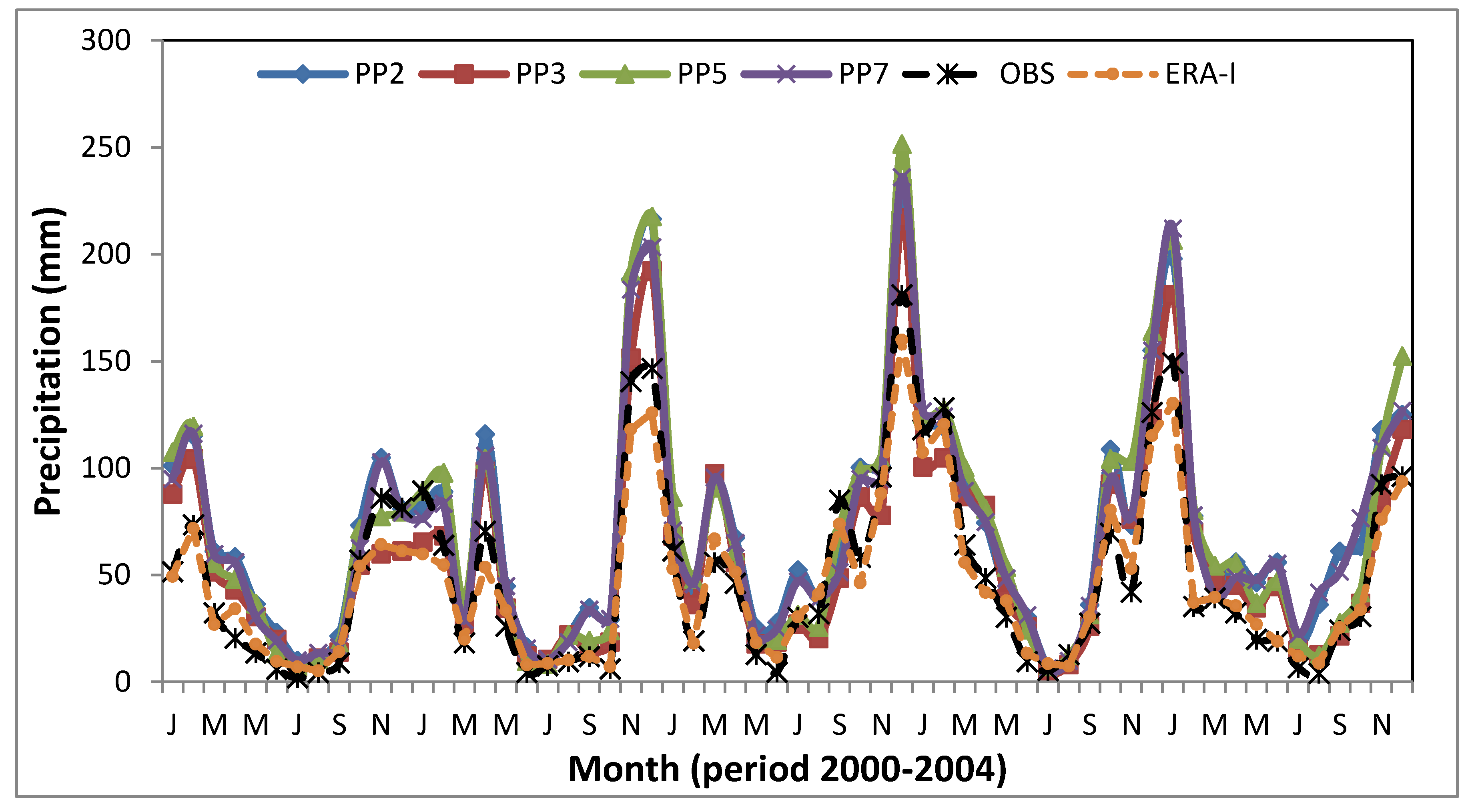
Monthly precipitation time-series are illustrated in Figure 2. The seasonal pattern of monthly precipitation is well captured by the majority of the schemes, also observed in the study of García-Díez et al. [57], remarking the highest precipitation during winter and lowest during summer. The black, dashed line illustrates the seasonal variability of monthly precipitation derived from the average values of the available stations, which is noticed on the models results. There are obvious similarities in the precipitation patterns among all experiments and observed data for the 5 years of comparison, yielding smoothly the precipitation’s inter-annual variability, especially during the wettest months and summer periods characterized of limited rainfall. Some differences show that in general, there is an overestimation of precipitation compared to ground data for all setups, and this probably is caused by excessive wintertime precipitation [85]. On the other hand, ERA-Interim appears to underestimate winter precipitation from November to January. Some cases of precipitation’s underestimation are related to the PP3 setup during the study period, and as this simulation appears to have the less overestimation among setups.
This fact is also confirmed with the 5-yearly estimation of statistical errors based on daily precipitation values in Table 4, where PP3 shows the best performance, with positive percentage BIAS of about 19%, while the other models have values of over 40%. As being observed, RMSE, MAE and COR results as well show slightly better performance for PP3 compared to the other simulations. It is worthy to note that PP3 bias (19%) is significantly smaller than the ±50% reported in the Third Assessment Report of the Intergovernmental Panel on Climate Change by Giorgi et al. [86] for RCMs, and while not small, it is close to the range of the best performing RCMs shown in several studies [3,23,71,87]. PP3 uses the Betts–Miller–Janjic cumulus parameterization, WSM6 for microphysics, the Mellor–Yamada–Janjic as PBL scheme and Monin-Obukhov similarity theory (Table 1). Statistical metrics between ERA-Interim and the WRF results indicate some loss of performance in the WRF model, with an underestimation of 5.5% PBIAS value in the total of stations’ grid points.
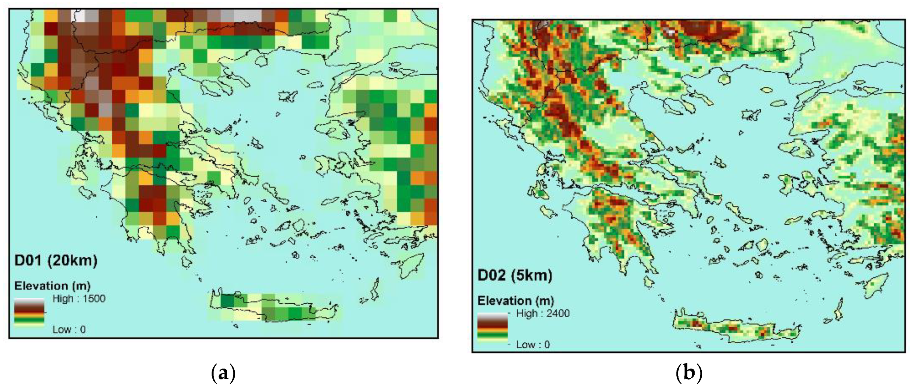
The study of the spatial distribution of 5-annual mean precipitation in WRF simulations and observations shows a clear topographical dependency (Figure S1). The analysis of the amount of precipitation yields large differences between plain areas and higher elevations, with maximum values of annual precipitation found in the western part of the country, related to fronts passages with increased vertical lift due to orographic enhancement in mountainous locations. All simulations depict similarly the spatial pattern of precipitation, with excessive rain being observed only in mountainous locations; however, there are no representative stations to validate such precipitation amounts. The same behavior is observed for all model setups, although PP7 seems to produce higher amounts of precipitation during the examined 5-year period than PP2 and PP3. This fact could be related to the interaction of the microphysical scheme with the association of PBL (MYJ) scheme, which is in line with other studies with higher precipitation totals and more convective precipitation [88,89]. Additionally, for precipitation over areas of complex topography, wet bias is particularly found to be common to several RCMs [90,91], and is probably caused by an overestimation of orographic precipitation enhancement [92], and/or to an inaccurate PBL simulation [7,11,93].
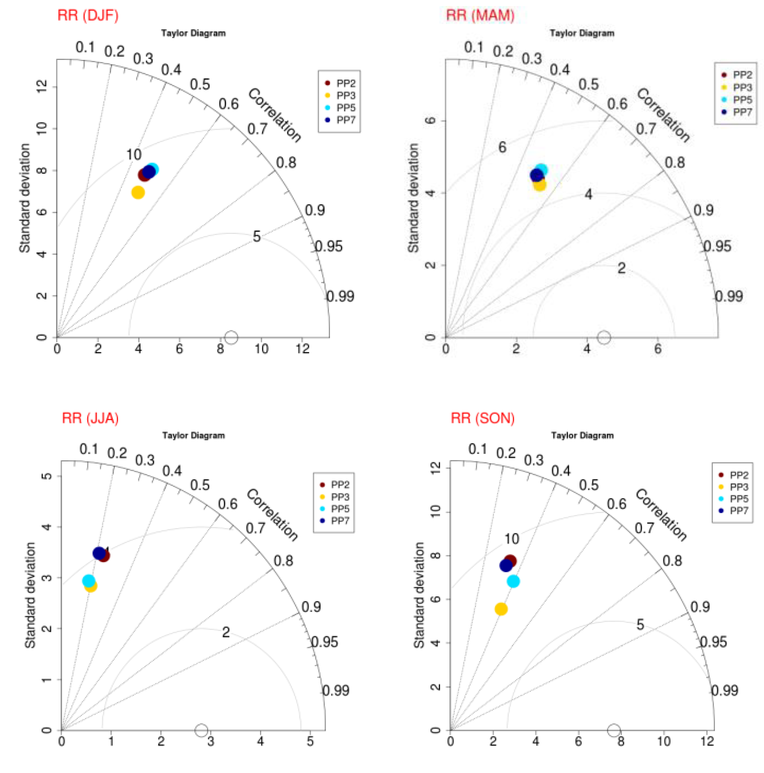
The Taylor diagrams shown in Figure 3 provide the comparative assessment of the four different model experiments to the choice of the physical parameterizations, to simulate the seasonal spatial pattern of daily precipitation during the examined period. The simulated results are compared to all observational data from 23 stations. The best simulation is marked by the largest correlation, smaller CRMSE and being closer to the observed standard deviation. It is found that the highest correlation in the range of 0.5–0.6 is observed during the winter and spring seasons, with the poorest correlation in summer, resulting though in the lowest centered RMSE values (~3.5 mm). It is well-known that the satisfied representation of summer precipitation is a demanding field for any model, and as the convective processes prevail, it is not easy to determine confidently the appropriate cumulus scheme. The poor performance of model setups is observed during winter and autumn, where the highest CRMSE values are displayed. All models’ simulations seem to have similar performance; however, PP3 appears to have slightly lowest errors during all seasons, thus yielding a better performance compared to the rest of the setups.
Because of the heterogeneous spatial pattern of precipitation in Greece, which is strongly associated with the orography, the extended coastline (see Figure 4) and the limited number of stations for comparison, statistical errors are also displayed per station in detail in Figure S4.
This analysis allows also exploring which of the simulations outperforms by station, which of the stations statistically is better validated from the WRF model, and finally which setup represents outmost the majority of the stations in Greece.
It is evident that the prevailing simulation with the lowest errors among stations is represented by PP3, showing a significant improvement regarding the others.
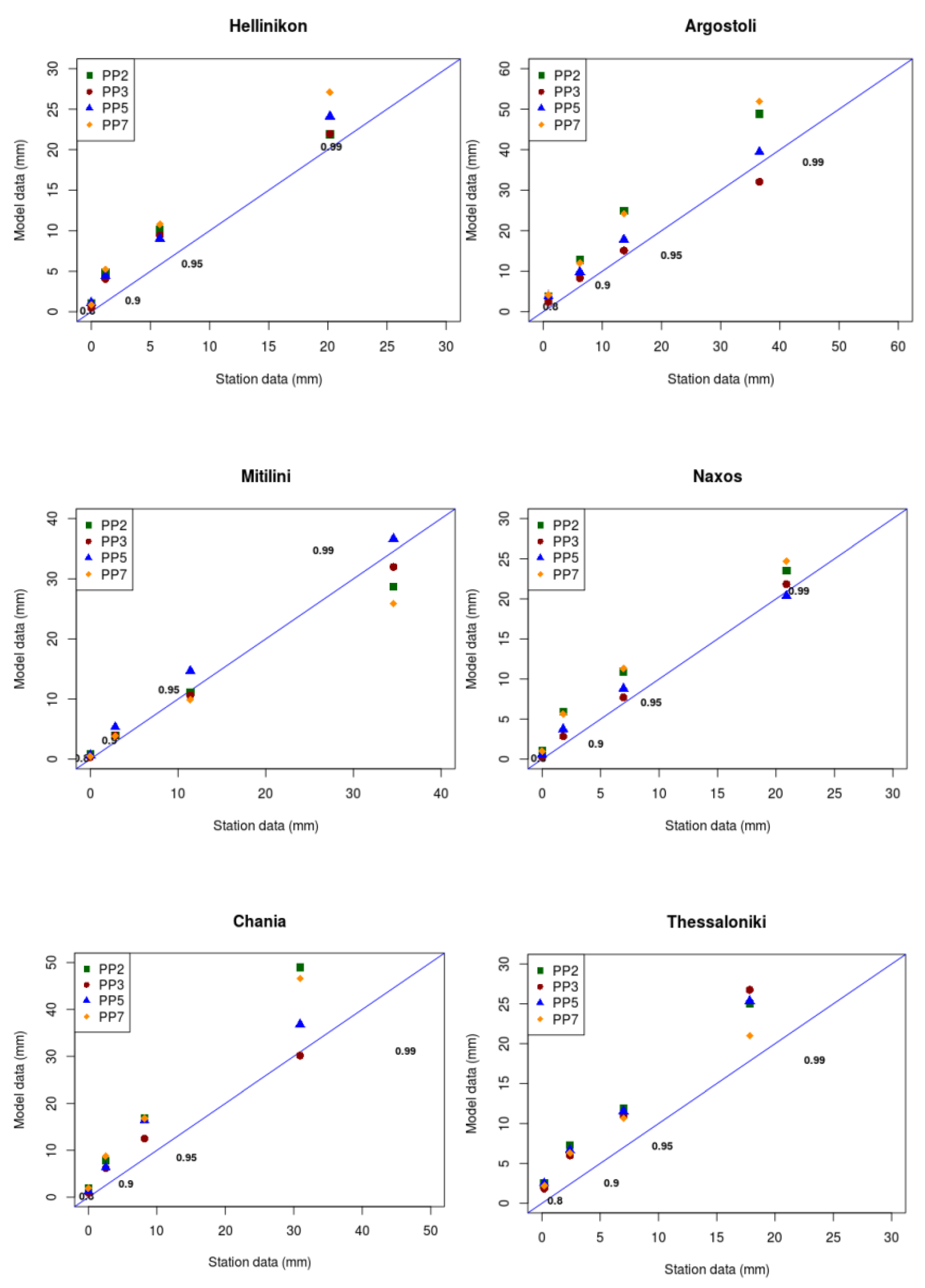
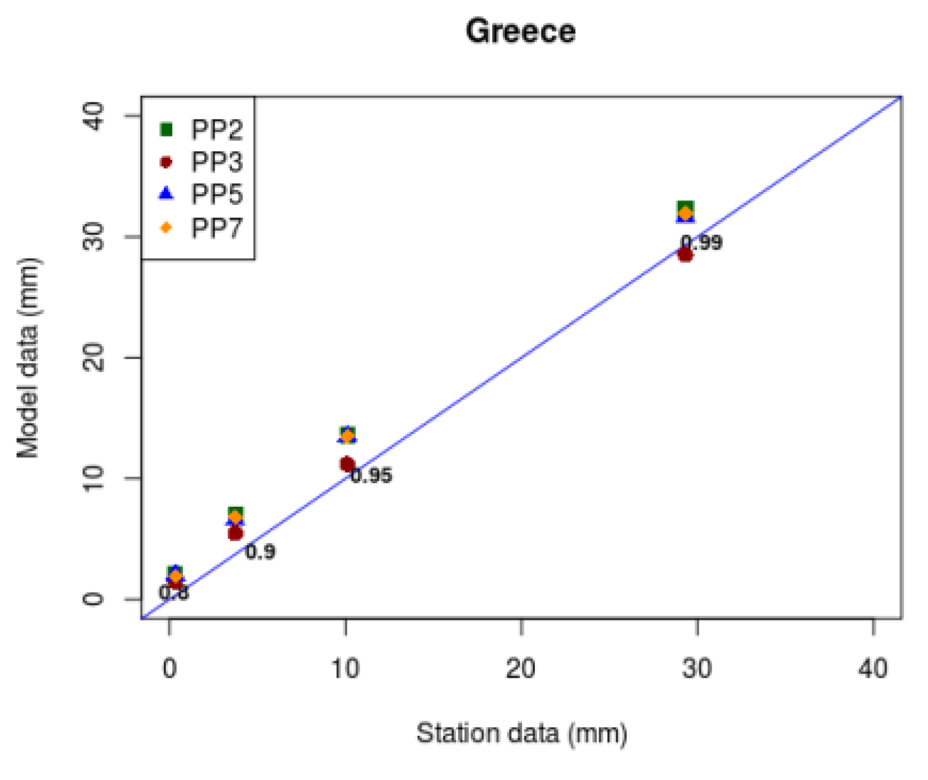
In general, regional models still misrepresent daily precipitation and precipitation extremes because of resolution or/and parameterization deficiencies [3]. The precipitation analysis was extended on studying the intensity of daily precipitation; thus, the 80th, 90th, 95th and 99th higher ranking percentiles were calculated. This analysis is very important for climate change assessment related to extreme weather events, drought and flooding events, that have significant socioeconomic impacts on the global community. The results are shown in Figure 5, where the WRF percentiles distribution is plotted versus the observational data for the domain of Greece and several indicative stations distributed all over Greece during these 5 years. The straight (blue) line depicts a perfect performance, indicating the over- or under-estimation of the simulated values compared to the observations.
The percentiles, obtained for the area of Greece, show that all WRF simulations follow very well the observational percentiles. The PP3 model setup outperforms remarkably well the extreme percentile 99%, while the other setups tend to slightly overestimate rainfall for 90% and 95% extremes. A general inspection of the percentiles results by station shows that WRF dynamical downscaling simulations overestimate extreme precipitation events, with few exceptions regarding the 99% percentile, and also that PP3 model simulation tends to reproduce rainfall extremes better than the other setups. In Table 5, precipitation verification statistics are presented in the contingency table for four distinct threshold values of precipitation compared to the 5-year observational data. This table depicts the results by station, only for the best performed simulation PP3. The forecasts show reasonable skills for both low and medium intensity rainfall days, as the model runs show POD values of (0.7–0.86) and (0.6–0.85), respectively. Regarding extreme rainfall events, the majority of the stations indicate POD values close to 0.5–0.6, followed by FAR values of (0.5–0.7), meaning that a very low percentage of these rain events (observed and/or predicted) were correctly forecast. Probably the rare episode of convective precipitation is often missed or underestimated by the model and the convective scheme.
3.2. Maximum Temperature/Minimum Temperature
Annual and seasonal changes in the daily minimum (TN) and maximum (TX) temperatures for the selected period have been analyzed. In general, it was found that physics parameterizations appear to have less noticeable effect on temperature than on precipitation [56].
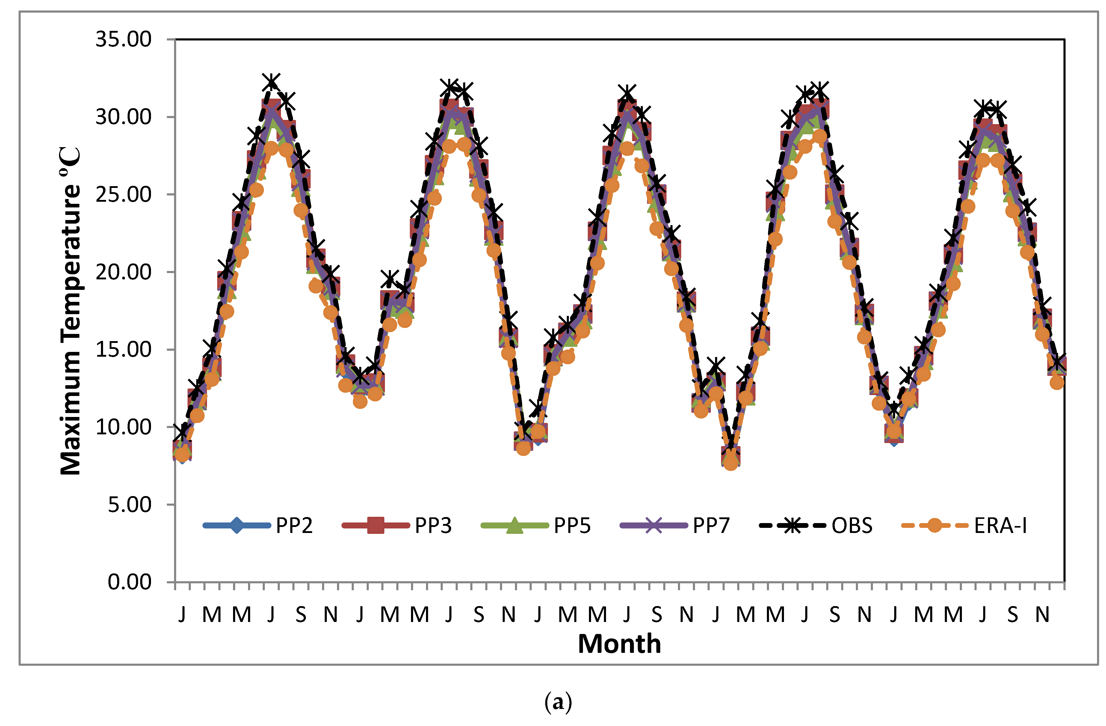
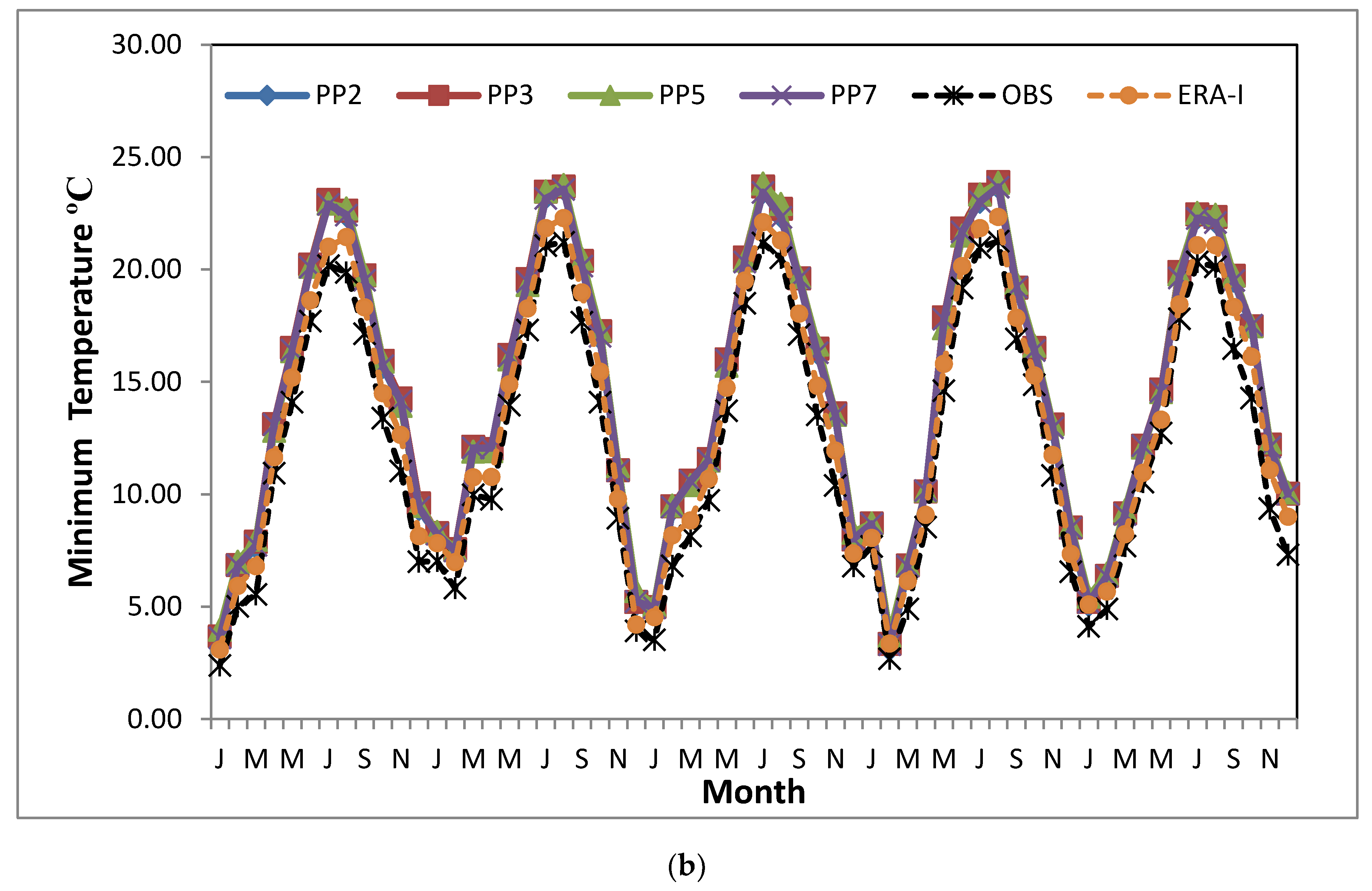
In Figure 6, the inter-annual cycle of daily-average minimum and maximum values of temperature by month is displayed for the total number of grid stations‘ points for the whole region of the study. The colored lines show the results of the simulations, and the dashed, black lines indicate observational data. In general, the observational seasonality is precisely captured during 2000–2004, while the summer/winter peaks are clearly identified as well. Similar representation and behavior of temperatures are observed regarding all physical schemes. Both temperature measures are in agreement over the study period, but WRF TX results are consistently colder, while TN is much warmer than observational data for all physical schemes. This bias appears to result mainly from the summertime over-prediction of daily-minimum temperature and summertime under-prediction of TX; daily-maximum biases tend to be smaller in magnitude and seasonally invariant, while the warm bias is mainly confined to the maximum temperatures. Additionally, the spatial distribution (Figure S2) of the simulated 5-years mean that the daily TX is characterized normally by a warm decreasing gradient from the coasts and low altitudes regions to mountainous chains, verified by the weather station values in spite of the limited number of observational data. Similar results are observed for minimum temperature as well (not shown). ERA-interim also performed well the inter-annual cycle for both temperatures, indicating lower values than the observed and modeled values during summer maximum values in the case of maximum temperature.
Table 6 presents the statistical metrics calculated for daily values. A high correlation coefficient of 0.96 is observed between the station and the simulated daily maximum temperature TX, with an overall negative BIAS from −1.1 to −1.4 °C, indicating a slightly better performance of the model for the PP3 (−1.06 °C) simulation.
The RMSE and MAE errors have values close to 2.6 °C and 2 °C, respectively, with similar values found for all simulations. Regarding the daily TN, a high correlation coefficient of 0.92 is observed between observations and model data, with a consistent positive bias of around 2 °C, ~3.5 °C RMSE and ~ 2.7 °C MAE values. These findings are in good agreement with high resolution climate analysis for temperature by Berg et al. [4] for Germany, and little higher values regarding RMSE/MAE values, (especially in the case of TX BIAS, which is found negligible −0.4 °C) in a similar study of Soares et al. [3] for Portugal. The results showed an improvement in maximum temperature with respect to the ERA-Interim dataset, and higher bias regarding minimum temperature, but without significant discrepancies on the other statistical errors.
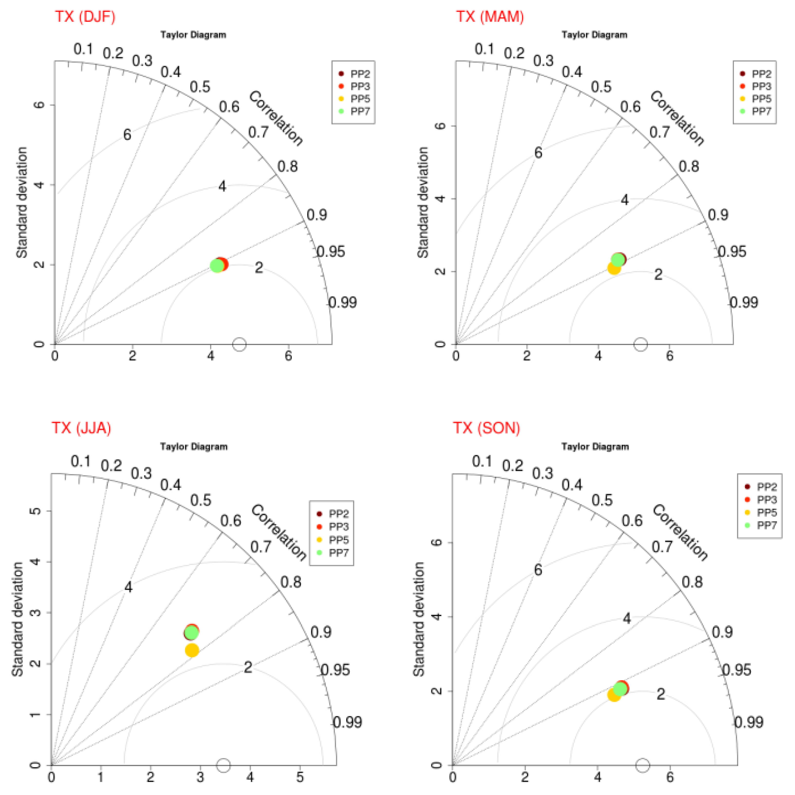
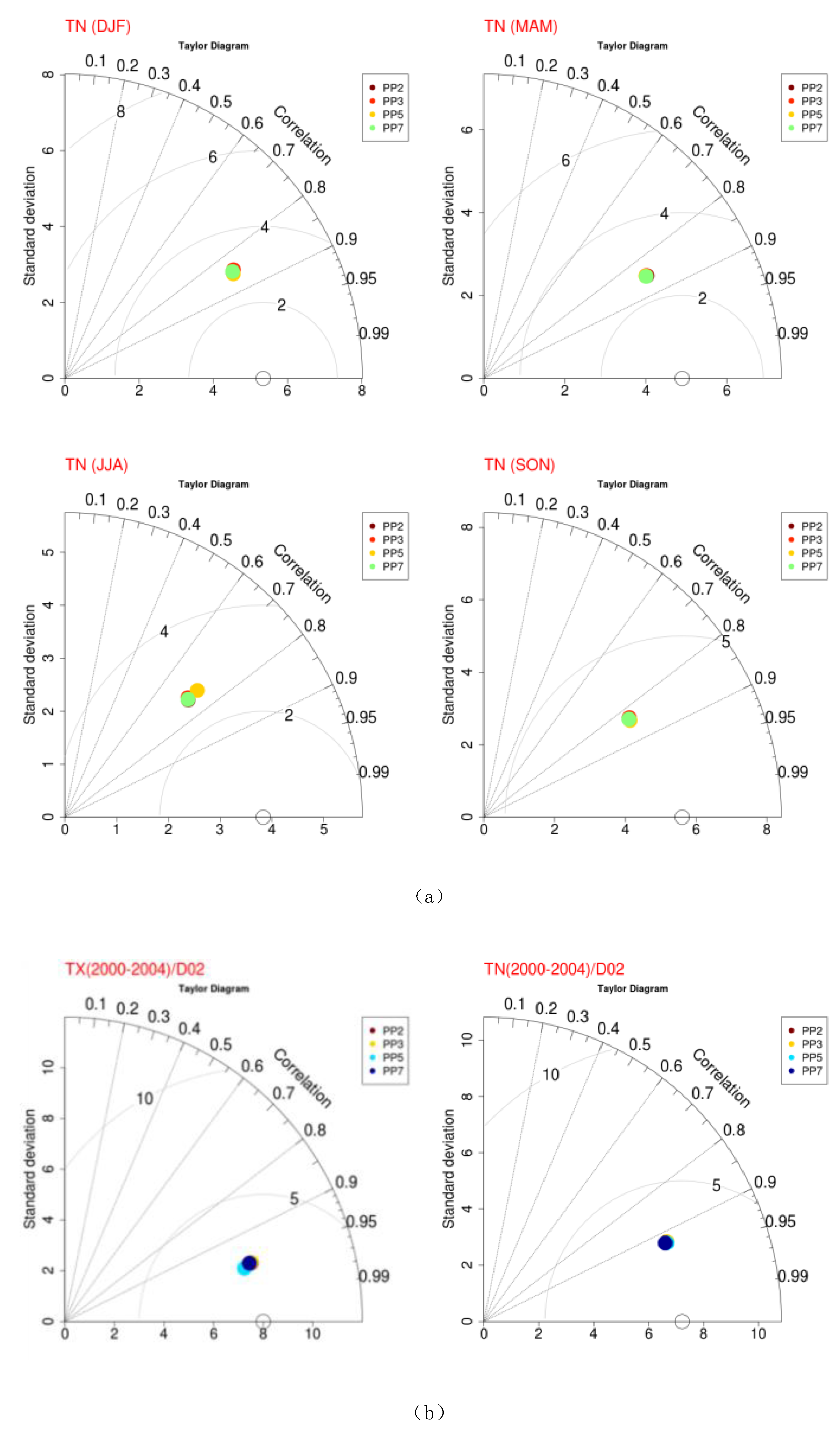
An overall performance of the simulations is illustrated in Figure 7 by Taylor plots for seasonal periods (winter, spring, summer and autumn - 7a) and annual (7b) during 2000–2004.
The diagrams for maximum temperature showed a good match between model results and observations at seasonal time scales. The lowest performance was obtained during the summer months, with correlations close to 0.75 that increase to 0.8 for PP5 simulation results. In addition, in the representation of metrics by station in Table 5, high RMSE values are observed, of about 3–3.5 °C for several stations. It was found in the initial study [26] that the cell of the certain model points that correspond to the location of the observed stations is characterized by the sea dominant land use category (e.g., Corfu, Heraklion, Mitilini, Argostoli etc.), and consequently during summer period could affect the results, with higher differences in temperature leading to stronger sea-land interaction in combination with the appearance of more intense thermal instability.
The correlations in the other seasons are much higher in the range of 0.9–0.95, and lower errors are observed with very similar values for all models. The Taylor diagram in a yearly time scale showed a very good agreement of models performance, with no distinct differences among them during the 5-year period. The correlation coefficient results showed a good match with values above 0.9 arising in the climatological study of Marta-Almeida et al. [94] for seasonal time scales in Spain.
Minimum temperatures showed a slightly lower performance than TX, with correlation values around 0.85 during spring, autumn and winter regarding all simulations results, while during summer months, a correlation lower than 0.8 is observed with no significant changes with respect to errors. A good agreement with observations is also found, and no significant statistical differences are yielded among PPs models for TN, as illustrated in the Taylor plot of Figure 7b with respect to the yearly timescale. The values of the correlations are higher than 0.9, as an increasing number of days were averaged. It is noticed that for all simulations the correlation coefficients of TN yield lower values (0.92–0.93) for high resolution domains, which is in agreement with other works [3,71]. It could be deduced that the model performs better for TN with the PP2 scheme with positive BIAS near 2 °C.
Table 7 depicts the best setup based on the daily values of statistical metrics BIAS (not shown), RMSE, MAE and the correlation coefficient (not shown) for the daily maximum temperature separately for each of the 28 stations, during the 5 years and the four different experiments. These same calculations were derived as well as for TN (not shown). Some exceptions in Table 5 concern 6–7 stations, that their BIAS is in the range of 2–3.5 °C, and probably is related to the selection of the nearest model point to station that is not located in land cell, or displays a significant height difference. From this analysis, it is evident that the setup that statistically outperforms with the lowest errors among stations is PP3, showing a significant improvement regarding the others, and thus representing the majority of the stations in Greece.
The range of errors appears to have values of 1.2 to 4 °C. It is also observed that the underestimation of the model is consistent for the entire area, and is close to −1.2 °C for the majority of the observational stations used in this comparison.
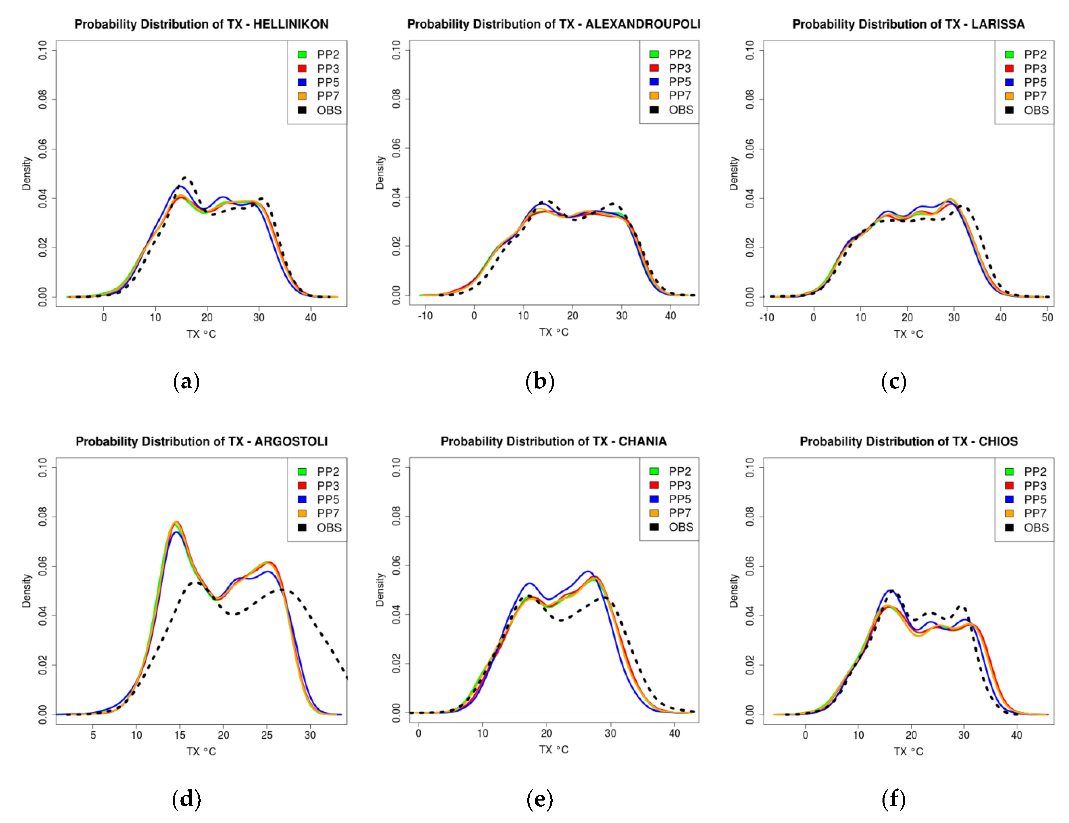
The comparison of model results and observations in terms of probability distribution (see Figure 8) for some indicative stations (for all stations see Figure S3) shows satisfied agreement for the majority of the stations for the 5-year period daily TX, as all WRF simulations follow the pattern distribution of observed data without having distinct differences among setups.
In a few stations, a lower model observations correspondence is found. More specifically, the Argostoli, Corfu, Florina, Heraklion, Kithira, Methoni, Milos and Mitilini stations illustrate a large shift towards colder values in the medium temperature range with higher density values. In Chania station all simulations appear to have higher density values for hotter temperatures, while in Ierapetra, the opposite behavior is observed. On the other hand, the TN probability distributions of WRF simulations (not shown), appear to have a large shift towards hotter values in the temperature range corresponding to either higher or lower density. This behavior justifies the consistent model’s overestimation, especially during the summer period.
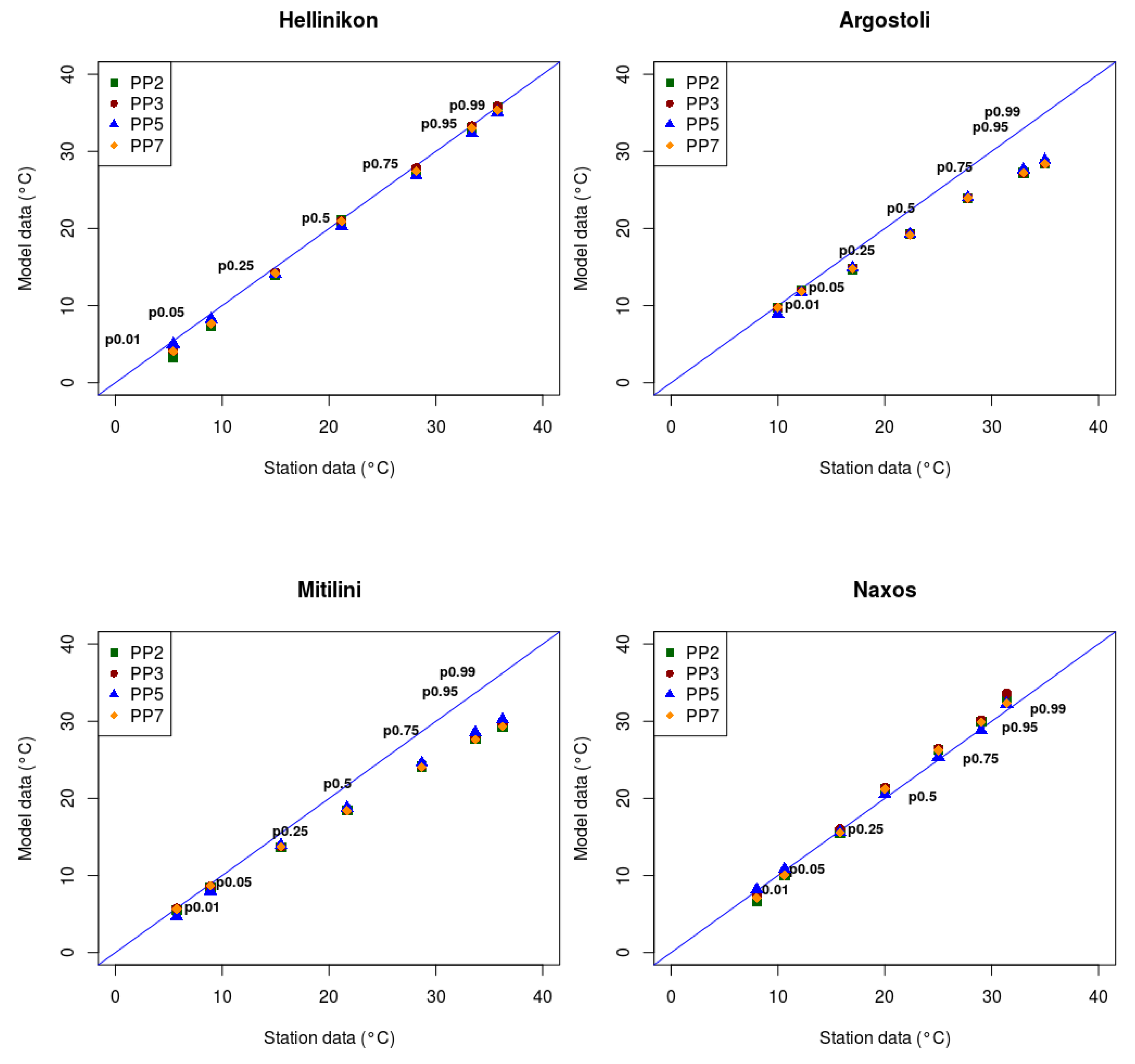
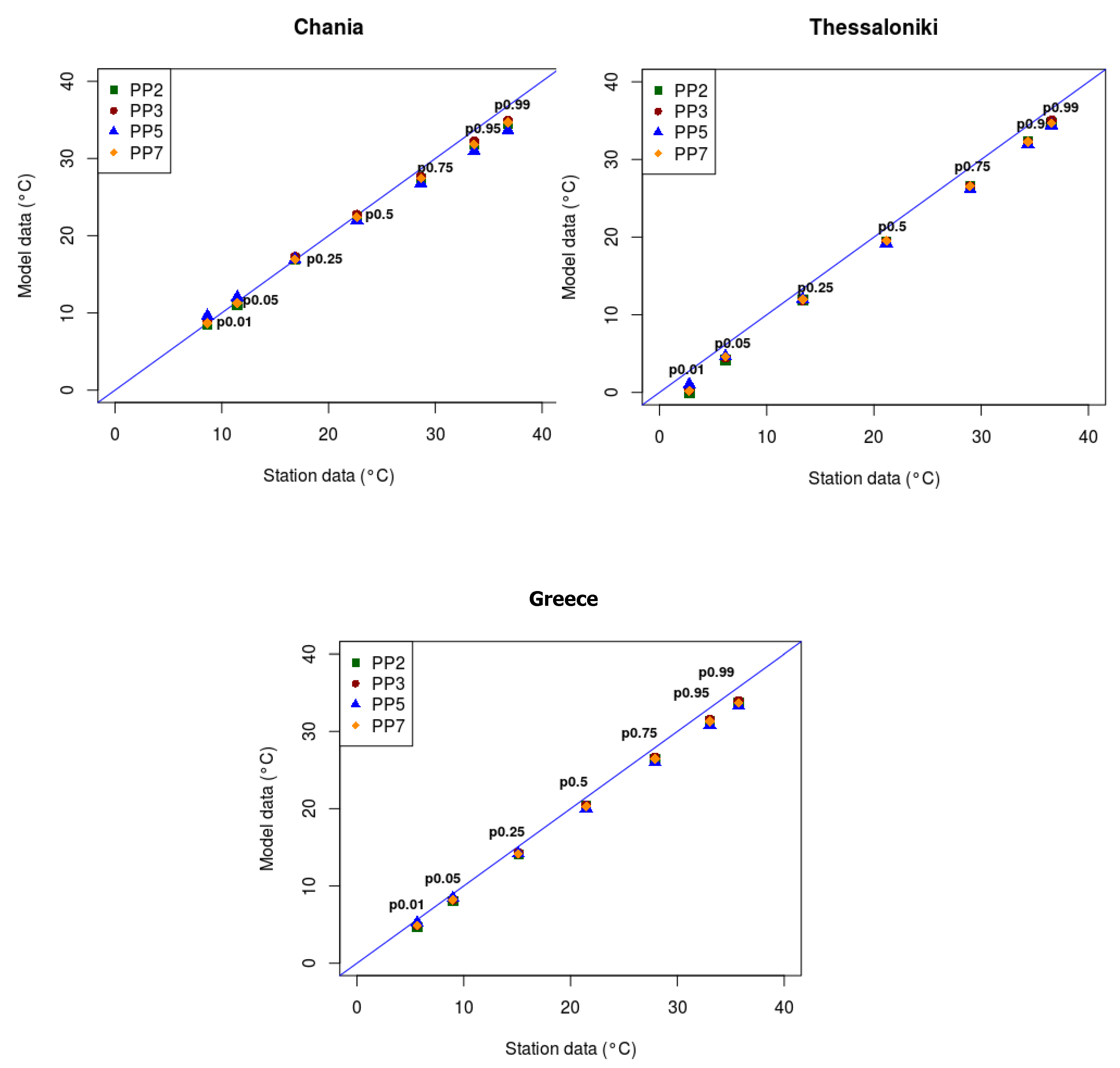
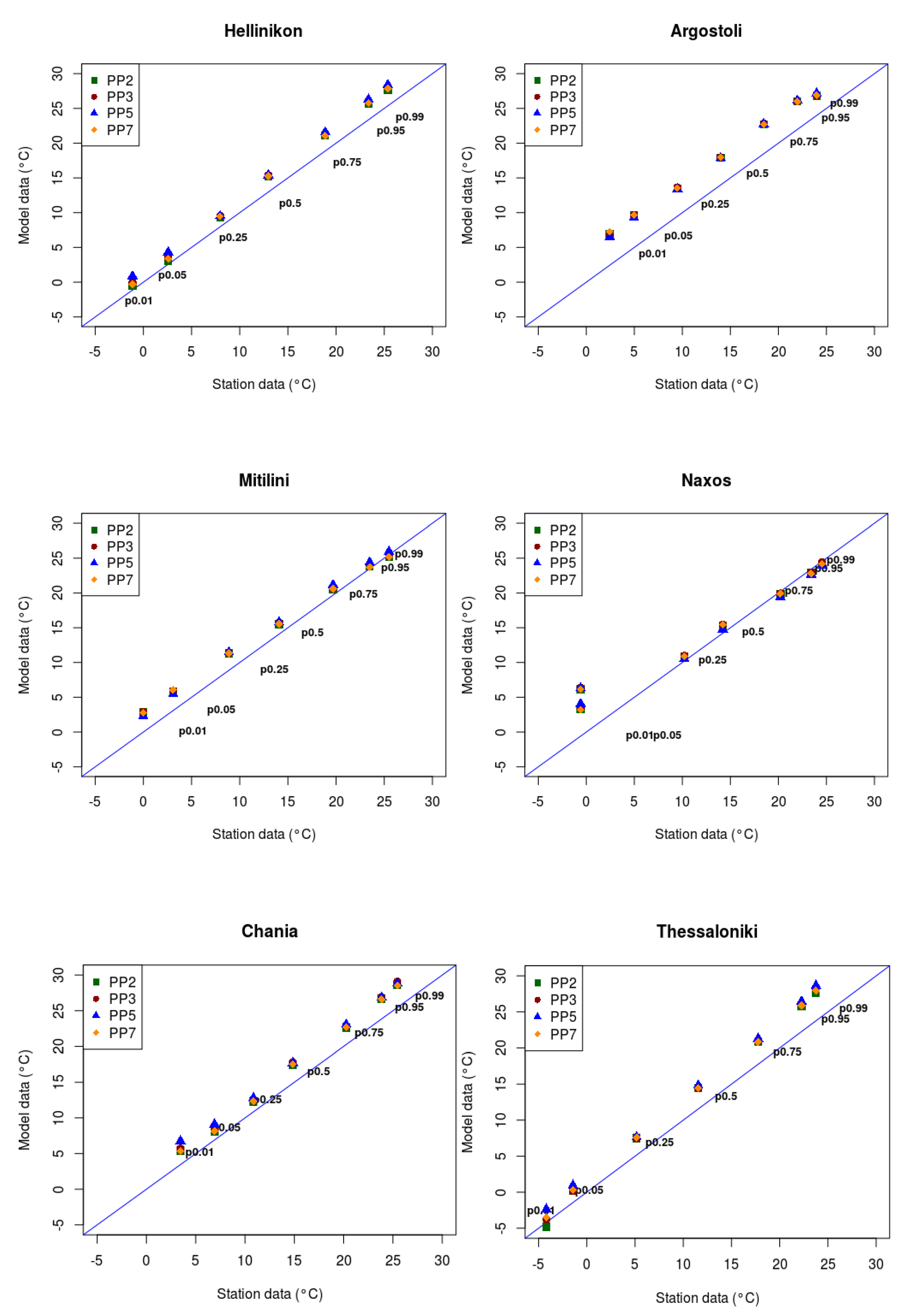
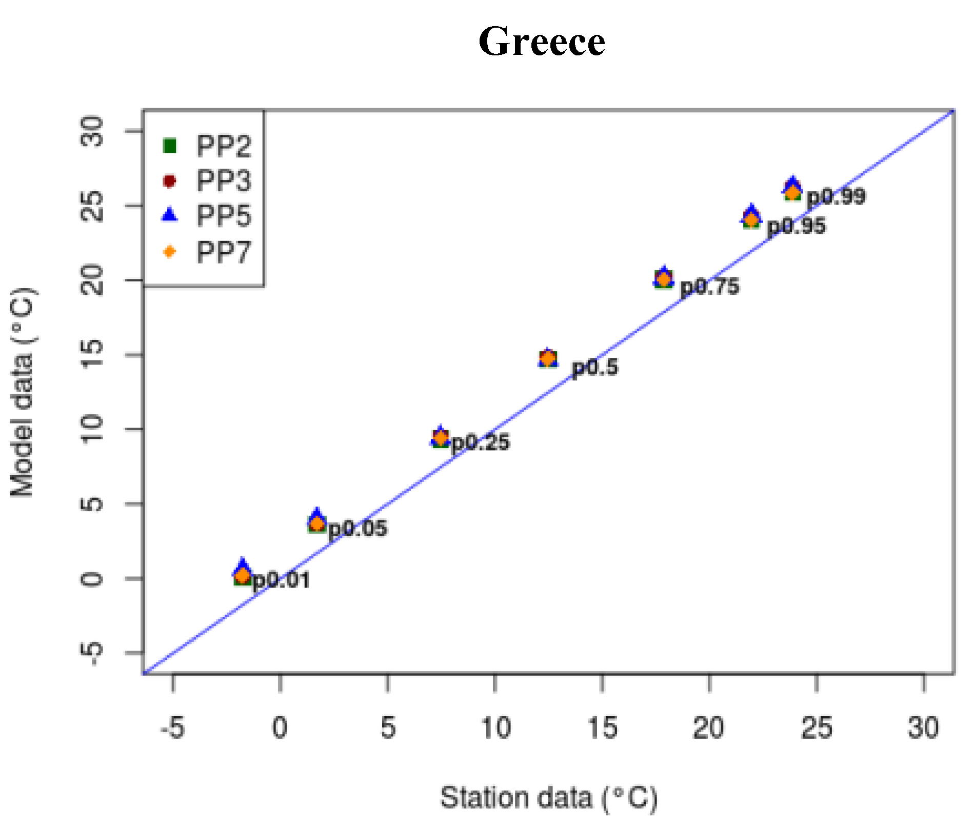
Percentiles of TX and TN (the 1st, 5th, 25th, 75th, 95th and 99th) of daily values for the 28 stations, as well as for the total region of Greece were calculated, in order to focus on the examination of extremes description by the different simulations. Percentiles for the WRF simulations versus observational percentiles are shown indicatively in Figure 9 and Figure 10, for TX and TN for several stations, and their average through the domain of Greece. As in the case of precipitation, the over- or underestimation of the simulations is indicated by the blue line, which represents the perfect description. It is evident that the maximum temperature is very well reproduced by WRF, with no significant differences between the different simulations, and with slight underestimation mostly for percentiles higher than 50%. There are some stations, e.g., Argostoli or Mitilini, that appear to have larger deviations in the extreme percentiles, and others like Naxos that show very good performances in predicting the extremes. In accordance, regarding the minimum temperature, all models’ setups indicate no significant differences in simulating percentiles as well, however in what concerns their behavior an almost systematic overestimation, is observed overall. Probably, as Pérez et al. [56] point out in the case study of the Canary Islands, these deviations could be due to the insufficient temperature correction on the representation of mountainous areas, because the altitude difference between the model and stations points has strong influence.
From the set of the simulations carried out in this study, obvious similarities were found in the precipitation patterns among simulations and observations during the 5-yr period, verifying smoothly the precipitation’s inter-annual variability, especially during the wettest months and summer periods. Additionally, the lowest positive percentage BIAS of about 19% was calculated for the selected combination of physics parameterizations PP3, while for the rest of the setups, values of over 40% were obtained, highlighting as the best configuration for the simulation of precipitation in the PP3 setup. Furthermore, all simulations regarding the maximum temperature demonstrated improved statistical metrics with respect to ERA-Interim data, and not significant differences in the case of the minimum temperature. Although some verification results among ERA-Interim and the WRF results indicated some loss of model performance for daily precipitation, the results demonstrated the necessity to use a high resolution RCM model for climate studies in Greece, due to the difficult geomorphology of the region (complex orography, irregular coastlines and regions with heterogeneous land cover).
Statistical analysis of the maximum and minimum temperatures for all tested simulations showed satisfactory results, characterized by a good match between modeled and observed data, with high correlation above 0.9, negative bias around 1–1.5 °C, and a positive bias of around 2 °C, respectively. Moreover, good performance was deduced with regards to the examination of extreme percentiles for temperatures and precipitation, with some deviation due to complex topography. PP3 showed a slightly better performance for the maximum temperature in the majority of the stations, while PP2 for the minimum temperature.
Given the small discrepancies between the results of these two setups in temperatures, and taking into account the noticeable difference in the results of PP3 for precipitation, we recommend PP3 as a good choice for the upcoming climate simulations. Several studies have supported the PP3 WRF setup (MYJ, WSM6, RRTMG, NOAH, BMJ) for climate or forecasting applications as overall, more balanced behavior is displayed for both surface variables; the annual precipitation cycle is captured adequately, and closer agreement with the observational datasets is found regarding temperatures and their extreme values [2,37,38,39,44,88,94,95].
It should be mentioned that this study was based on previous research that has already examined a combination of physics parameterizations, and performed sensitivity tests for the area of interest, analyzing the effect of the chosen schemes; therefore an in-depth analysis of physical scheme inter-comparison was not in the scope of the current work. The use of RCMs for the simulation of historical, current and future climate, particularly in view of the warming climate, is continuously increasing, as it is considered important for studying regional climate changes. It is considered important to emphasize that the current study aimed at identifying an appropriate WRF model set up in order to perform in the future high-resolution historical climatology simulation, by downscaling ERA-interim reanalysis to the domain of Greece. For the realization of the future work related to the hindcast evaluation of the WRF model, different interpolation methods will be considered for the determination of the nearest model points to the stations to decrease statistical errors, particularly for those located within coastal and mountainous areas. In the future analysis, we will also consider the application of bias correction methods to reproduce more reliable results regarding precipitation. Additionally, according to Emery [96], if the mean error for temperature exceeds the ±0.5 threshold, it is suggested to adjust bias correction methodologies, before the results are applied to other studies.
4. Conclusions
In this study, we performed a preliminary investigation on high resolution (5 km × 5 km) regional climatology over the domain of Greece, by downscaling 5-years ERA-Interim reanalysis data using the WRF model. The dynamical downscaling was performed using in total four different setups to investigate the model performance for precipitation and surface maximum and minimum temperature variables that are relevant to climate impact studies. The results were compared with the observational data of HNMS through detailed statistical analysis. As there were no available high resolution observational gridded datasets, the comparison of the simulations was realized through the closest model grid point of the inner domain to the station. In general, clear similarities were found in the precipitation patterns among simulations and observations, yielding the lowest positive percentage BIAS calculated at about 19% for the PP3 setup. Overall, this PP3 model simulation reproduced rainfall extremes better than the other setups, even though the model overestimated extreme precipitation events with few exceptions regarding the 99% percentile. The same conclusion was drawn for maximum and minimum temperatures, as PP3 simulations yielded the lowest statistical errors for the majority of the stations.
Within its limitations, the study advocates that the PP3 model setup, which corresponds to the combination of physics schemes, including WSM6, MYJ, and BMJ, is suitable for high resolution climate modeling studies (hindcast and future climate scenarios runs) for the domain of Greece, as the specific parameterization schemes simulate better the temperature and precipitation fields compared to the rest of the investigated setups.
Supplementary Materials
The following are available online at https://0-www-mdpi-com.brum.beds.ac.uk/2225-1154/8/3/44/s1.
Author Contributions
Conceptualization, N.P., A.S. and D.V.; methodology, N.P and A.S.; software, N.P. and S.K.; validation, N.P.; formal analysis, N.P.; investigation, N.P., D.V. and A.S.; writing—original draft preparation, N.P.; writing—review and editing, D.V. and A.S.; visualization, N.P.; supervision, P.T.N., D.V. and A.S. All authors have read and agreed to the published version of the manuscript.
Funding
“This research has been co-financed by the European Regional Development Fund of the European Union and Greek national funds through the Operational Program Competitiveness, Entrepreneurship and Innovation, under the call RESEARCH–CREATE–INNOVATE (project code:T1EDK- 02219) ”.
Acknowledgments
We acknowledge the data providers in the ECA and D project (http://www.ecad.eu). We kindly acknowledge Rita M. Cardoso and Pedro M. M. Soares from the Insituto Dom Luiz of University of Lisbon (Portugal) for their advice and guidance. This work was supported by computational time granted from the Greek Research and Technology Network (GRNET) in the National HPC facility, ARIS, under project ID HRCOG (pr004020).
Conflicts of Interest
The authors declare no conflict of interest. The funders had no role in the design of the study; in the collection, analyses, nor interpretation of data; in the writing of the manuscript, nor in the decision to publish the results.
References
- El-Samra, R.; Bou-Zeid, E.; El-Fadel, M. What model resolution is required in climatological downscaling over complex terrain? Atmos. Res. 2018, 203, 68–82. [Google Scholar] [CrossRef]
- Argüeso, D.; Hidalgo-Muñoz, J.M.; Fortis, S.R.G.; Esteban-Parra, M.J.; Dudhia, J.; Castro-Díez, Y. Evaluation of WRF Parameterizations for Climate Studies over Southern Spain Using a Multistep Regionalization. J. Clim. 2011, 24, 5633–5651. [Google Scholar] [CrossRef]
- Soares, P.M.M.; Cardoso, R.M.; Miranda, P.; De Medeiros, J.; Belo-Pereira, M.; Espirito-Santo, F. WRF high resolution dynamical downscaling of ERA-Interim for Portugal. Clim. Dyn. 2012, 39, 2497–2522. [Google Scholar] [CrossRef]
- Berg, P.; Wagner, S.; Kunstmann, H.; Schädler, G. High resolution regional climate model simulations for Germany: part I—validation. Clim. Dyn. 2013, 40, 401–414. [Google Scholar] [CrossRef]
- Wang, J.-J.; Adler, R.F.; Huffman, G.J.; Bolvin, D. An Updated TRMM Composite Climatology of Tropical Rainfall and Its Validation. J. Clim. 2014, 27, 273–284. [Google Scholar] [CrossRef] [Green Version]
- Wang, J.; Kotamarthi, V.R. High-resolution dynamically downscaled projections of precipitation in the mid and late 21st century over North America. Earth’s Futur. 2015, 3, 268–288. [Google Scholar] [CrossRef]
- Xu, Z.; Yang, Z. A new dynamical downscaling approach with GCM bias corrections and spectral nudging. J. Geophys. Res. Atmos. 2015, 120, 3063–3084. [Google Scholar] [CrossRef]
- Prein, A.F.; Gobiet, A.; Truhetz, H.; Keuler, K.; Goergen, K.; Teichmann, C.; Fox Maule, C.; van Meijgaard, E.; Déqué, M.; Nikulin, G.; et al. Precipitation in the EURO-CORDEX 0.11◦ and 0.44◦ simulations: high resolution, high benefits. Clim. Dyn. 2016, 46, 383–412. [Google Scholar] [CrossRef]
- Kryza, M.; Wałaszek, K.; Ojrzyńska, H.; Szymanowski, M.; Werner, M.; Dore, A.J. High-Resolution Dynamical Downscaling of ERA-Interim Using the WRF Regional Climate Model for the Area of Poland. Part 1: Model Configuration and Statistical Evaluation for the 1981–2010 Period. Geoinform. Atmos. Sci. 2017, 174, 53–68. [Google Scholar] [CrossRef] [Green Version]
- El-Samra, R.; Bou-Zeid, E.; El-Fadel, M. To what extent does high-resolution dynamical downscaling improve the representation of climatic extremes over an orographically complex terrain? Theor. Appl. Clim. 2017, 134, 265–282. [Google Scholar] [CrossRef]
- Xu, Z.; Han, Y.; Yang, Z. Dynamical downscaling of regional climate: A review of methods and limitations. Sci. China Earth Sci. 2018, 62, 365–375. [Google Scholar] [CrossRef]
- Sørland, S.L.; Schar, C.; Lüthi, D.; Kjellström, E.; Luethi, D. Bias patterns and climate change signals in GCM-RCM model chains. Environ. Res. Lett. 2018, 13, 074017. [Google Scholar] [CrossRef]
- Giorgi, F.; William, J.G., Jr. Regional Dynamical Downscaling and the CORDEX Initiative. Annu. Rev. Environ. Resour. 2015, 40, 467–490. [Google Scholar] [CrossRef]
- Giorgi, F.; Gao, X. Regional earth system modeling: review and future directions. Atmos. Ocean. Sci. Lett. 2018, 11, 189–197. [Google Scholar] [CrossRef] [Green Version]
- Jacob, D.; Petersen, J.; Eggert, B.; Alias, A.; Christensen, O.B.; Bouwer, L.M.; Braun, A.; Colette, A.; Déqué, M.; Georgievski, G.; et al. EURO-CORDEX: new high-resolution climate change projections for European impact research. Reg. Environ. Chang. 2013, 14, 563–578. [Google Scholar] [CrossRef]
- Dosio, A. Projections of climate change indices of temperature and precipitation from an ensemble of bias-adjusted high-resolution EURO-CORDEX regional climate models. J. Geophys. Res. Atmos. 2016, 121, 5488–5511. [Google Scholar] [CrossRef]
- Dyrrdal, A.V.; Stordal, F.; Lussana, C. Evaluation of summer precipitation from EURO-CORDEX fine-scale RCM simulations over Norway. Int. J. Clim. 2017, 38, 1661–1677. [Google Scholar] [CrossRef]
- Lhotka, O.; Kyselý, J.; Plavcová, E. Evaluation of major heat waves’ mechanisms in EURO-CORDEX RCMs over Central Europe. Clim. Dyn. 2017, 50, 4249–4262. [Google Scholar] [CrossRef]
- Mascaro, G.; Viola, F.; Deidda, R. Evaluation of Precipitation from EURO-CORDEX Regional Climate Simulations in a Small-Scale Mediterranean Site. J. Geophys. Res. Atmos. 2018, 123, 1604–1625. [Google Scholar] [CrossRef]
- Berg, P.; Christensen, O.B.; Klehmet, K.; Lenderink, G.; Olsson, J.; Teichmann, C.; Yang, W. Summertime precipitation extremes in a EURO-CORDEX 0.11° ensemble at an hourly resolution. Nat. Hazards Earth Syst. Sci. 2019, 19, 957–971. [Google Scholar] [CrossRef] [Green Version]
- Ruti, P.; Somot, S.; Giorgi, F.; Dubois, C.; Flaounas, E.; Obermann, A.; Dell’Aquila, A.; Pisacane, G.; Harzallah, A.; Lombardi, E.; et al. Med-CORDEX Initiative for Mediterranean Climate Studies. Bull. Am. Meteorol. Soc. 2016, 97, 1187–1208. [Google Scholar] [CrossRef] [Green Version]
- Colmet-Daage, A.; Sanchez-Gomez, E.; Ricci, S.; LloveL, C.; Estupina, V.B.; Quintana-Seguí, P.; Llasat, M.C.; Servat, É. Evaluation of uncertainties in mean and extreme precipitation under climate change for northwestern Mediterranean watersheds from high-resolution Med and Euro-CORDEX ensembles. Hydrol. Earth Syst. Sci. 2018, 22, 673–687. [Google Scholar] [CrossRef] [Green Version]
- Heikkilä, U.; Sandvik, A.; Sorteberg, A. Dynamical downscaling of ERA-40 in complex terrain using the WRF regional climate model. Clim. Dyn. 2010, 37, 1551–1564. [Google Scholar] [CrossRef] [Green Version]
- Torma, C.; Giorgi, F.; Coppola, E. Added value of regional climate modeling over areas characterized by complex terrain-Precipitation over the Alps. J. Geophys. Res. Atmos. 2015, 120, 3957–3972. [Google Scholar] [CrossRef]
- Czernecki, B. Creating wind field time-series over the Southern Baltic area using a dynamical downscaling approach. Meteorol. Z. 2013, 22, 587–593. [Google Scholar] [CrossRef]
- Politi, N.; Nastos, P.; Sfetsos, A.; Vlachogiannis, D.; Dalezios, N. Evaluation of the AWR-WRF model configuration at high resolution over the domain of Greece. Atmos. Res. 2018, 208, 229–245. [Google Scholar] [CrossRef]
- Ke, Y.; Leung, L.R.; Huang, M.; Li, H. Enhancing the representation of subgrid land surface characteristics in land surface models. Geosci. Model Dev. 2013, 6, 1609–1622. [Google Scholar] [CrossRef] [Green Version]
- Jung, G. Regional climate change and the impact on hydrology in the Volta Basin of West Africa. Doctoral Dissertation, University of Augsburg, Augsburg, Germany, 2006. [Google Scholar]
- Vigaud, N.; Pohl, B.; Crétat, J. Tropical-temperate interactions over southern Africa simulated by a regional climate model. Clim. Dyn. 2012, 39, 2895–2916. [Google Scholar] [CrossRef]
- Prein, A.F.; Holland, G.J.; Rasmussen, R.M.; Done, J.; Ikeda, K.; Clark, M.; Liu, C.H. Importance of Regional Climate Model Grid Spacing for the Simulation of Heavy Precipitation in the Colorado Headwaters. J. Clim. 2013, 26, 4848–4857. [Google Scholar] [CrossRef] [Green Version]
- Wagner, S.; Berg, P.; Schädler, G.; Kunstmann, H. High resolution regional climate model simulations for Germany: Part II—projected climate changes. Clim. Dyn. 2012, 40, 415–427. [Google Scholar] [CrossRef]
- Frei, C.; Christensen, J.H.; Déqué, M.; Jacob, D.; Jones, R.G.; Vidale, P.L. Daily precipitation statistics in regional climate models: Evaluation and intercomparison for the European Alps. J. Geophys. Res. Space Phys. 2003, 108. [Google Scholar] [CrossRef]
- Boberg, F.; Berg, P.; Thejll, P.; Gutowski, W.J.; Christensen, J.H. Improved confidence in climate change projections of precipitation further evaluated using daily statistics from ENSEMBLES models. Clim. Dyn. 2009, 35, 1509–1520. [Google Scholar] [CrossRef]
- Olsson, J.; Berg, P.; Kawamura, A. Impact of RCM Spatial Resolution on the Reproduction of Local, Subdaily Precipitation. J. Hydrometeorol. 2015, 16, 534–547. [Google Scholar] [CrossRef]
- Sunyer, M.A.; Luchner, J.; Onof, C.; Madsen, H.; Arnbjerg-Nielsen, K. Assessing the importance of spatio-temporal RCM resolution when estimating sub-daily extreme precipitation under current and future climate conditions. Int. J. Clim. 2016, 37, 688–705. [Google Scholar] [CrossRef] [Green Version]
- Pieri, A.B.; Von Hardenberg, J.; Parodi, A.; Provenzale, A. Sensitivity of Precipitation Statistics to Resolution, Microphysics, and Convective Parameterization: A Case Study with the High-Resolution WRF Climate Model over Europe. J. Hydrometeorol. 2015, 16, 1857–1872. [Google Scholar] [CrossRef]
- Cardoso, R.M.; Soares, P.M.M.; Miranda, P.; Belo-Pereira, M. WRF high resolution simulation of Iberian mean and extreme precipitation climate. Int. J. Clim. 2012, 33, 2591–2608. [Google Scholar] [CrossRef]
- Katragkou, E.; García-Díez, M.; Vautard, R.; Sobolowski, S.; Zanis, P.; Alexandri, G.; Cardoso, R.M.; Colette, A.; Fernández, J.; Gobiet, A.; et al. Regional climate hindcast simulations within EURO-CORDEX: evaluation of a WRF multi-physics ensemble. Geosci. Model Dev. 2015, 8, 603–618. [Google Scholar] [CrossRef] [Green Version]
- Ojrzyńska, H.; Kryza, M.; Wałaszek, K.; Szymanowski, M.; Werner, M.; Dore, A.J. High-Resolution Dynamical Downscaling of ERA-Interim Using the WRF Regional Climate Model for the Area of Poland. Part 2: Model Performance with Respect to Automatically Derived Circulation Types. Geoinform. Atmos. Sci. 2017, 174, 69–92. [Google Scholar] [CrossRef] [Green Version]
- Ojeda, M.G.-V.; Fortis, S.R.G.; Castro-Díez, Y.; Esteban-Parra, M.J. Evaluation of WRF capability to detect dry and wet periods in Spain using drought indices. J. Geophys. Res. Atmos. 2017, 122, 1569–1594. [Google Scholar] [CrossRef]
- Stanzel, P.; Kling, H. From ENSEMBLES to CORDEX: Evolving climate change projections for Upper Danube River flow. J. Hydrol. 2018, 563, 987–999. [Google Scholar] [CrossRef]
- Vlachogiannis, D.; Sfetsos, A.; Karozis, S.N.; Emmanouil, G.; Gounaris, N.; Mita, C. Mesoscale Simulation of hot weather events during august 2012 in Greece. In Proceedings of the Int. Conf. on Harmonisation within Atmospheric Dispersion Modeling for Regulatory Purposes, Madrid, Spain, 6–9 May 2013. [Google Scholar]
- Eleftheriadou, A.; Sfetsos, A.; Gounaris, N. The suitability of high resolution downscaled seasonal models for the energy assessment of the building sector. Energy Build. 2016, 111, 176–183. [Google Scholar] [CrossRef]
- Efstathiou, G.; Zoumakis, N.; Melas, D.; Lolis, C.; Kassomenos, P. Sensitivity of WRF to boundary layer parameterizations in simulating a heavy rainfall event using different microphysical schemes. Effect on large-scale processes. Atmos. Res. 2013, 132, 125–143. [Google Scholar] [CrossRef]
- Kartsios, S.; Kotsopoulos, S.; Karacostas, T.S.; Tegoulias, I.; Pytharoulis, I.; Bampzelis, D. Statistical evaluation of the simulated convective activity over Central Greece. In Proceedings of the Geophysical Research Abstracts EGU General Assembly 2015, Vienna, Austria, 12–17 April 2015; Volume 17, pp. 2015–8418. [Google Scholar]
- Pytharoulis, I.; Tegoulias, I.; Kotsopoulos, S.; Bampzelis, D.; Kartsios, S.; Zanis, P.; Katragkou, E.; Karacostas, T. High-Resolution WRF Hindcasts over the central Greece: Characteristics of simulated convective activity and model evaluation. In Proceedings of the 15th Annual WRF Users’ Workshop, Boulder, Colorado, USA, 25 June 2014. [Google Scholar]
- Giannaros, T.M.; Kotroni, V.; Lagouvardos, K. Predicting lightning activity in Greece with the Weather Research and Forecasting (WRF) model. Atmos. Res. 2015, 156, 1–13. [Google Scholar] [CrossRef]
- Available online: http://preprints.acmac.uoc.gr/314/1/acmac-0314.pdf (accessed on 16 March 2020).
- Matsangouras, I.T.; Nastos, P.; Pytharoulis, I. Synoptic-mesoscale analysis and numerical modeling of a tornado event on 12 February 2010 in northern Greece. Adv. Sci. Res. 2011, 6, 187–194. [Google Scholar] [CrossRef] [Green Version]
- Sindosi, O.A.; Bartzokas, A.; Kotroni, V.; Lagouvardos, K. Verification of precipitation forecasts of MM5 model over Epirus, NW Greece, for various convective parameterization schemes. Nat. Hazards Earth Syst. Sci. 2012, 12, 1393–1405. [Google Scholar] [CrossRef]
- Kotroni, V.; Lagouvardos, K. Evaluation of MM5 High-Resolution Real-Time Forecasts over the Urban Area of Athens, Greece. J. Appl. Meteorol. 2004, 43, 1666–1678. [Google Scholar] [CrossRef]
- Mazarakis, N.; Kotroni, V.; Lagouvardos, K.; Argiriou, A. The sensitivity of numerical forecasts to convective parameterization during the warm period and the use of lightning data as an indicator for convective occurrence. Atmos. Res. 2009, 94, 704–714. [Google Scholar] [CrossRef]
- Dee, D.P.; Uppala, S.M.; Simmons, A.J.; Berrisford, P.; Poli, P.; Kobayashi, S.; Andrae, U.; Balmaseda, M.A.; Balsamo, G.; Bauer, P.; et al. The ERA-Interim reanalysis: Configuration and performance of the data assimilation system. Q. J. R. Meteorol. Soc. 2011, 137, 553–597. [Google Scholar] [CrossRef]
- Skamarock, W.C.; Klemp, J.B.; Dudhia, J.; Gill, D.O.; Barker, D.M.; Duda, M.G.; Huang, X.Y.; Wang, W.; Power, J.G. A Description of the Advanced Research WRF Version 3; NCAR/TN-475+STR; National Center for Atmospheric Research: Boulder, CO, USA, 2008. [Google Scholar]
- Perez, J.C.; Diaz, J.P.; Gonzalez, A.; Exposito, F.J.; López, F.R.; Taima, D. Evaluation of WRF Parameterizations for Dynamical Downscaling in the Canary Islands. J. Clim. 2014, 27, 5611–5631. [Google Scholar] [CrossRef]
- Liu, P.; Tsimpidi, A.; Hu, Y.; Stone, B.; Russell, A.G.; Nenes, A. Differences between downscaling with spectral and grid nudging using WRF. Atmos. Chem. Phys. Discuss. 2012, 12, 3601–3610. [Google Scholar] [CrossRef] [Green Version]
- García-Díez, M.; Fernández, J.; Vautard, R. An RCM multi-physics ensemble over Europe: multi-variable evaluation to avoid error compensation. Clim. Dyn. 2015, 45, 3141–3156. [Google Scholar] [CrossRef] [Green Version]
- Lo, J.C.-F.; Yang, Z.; Pielke, R.A. Assessment of three dynamical climate downscaling methods using the Weather Research and Forecasting (WRF) model. J. Geophys. Res. Space Phys. 2008, 113, 09112. [Google Scholar] [CrossRef]
- Hahmann, A.N.; Vincent, C.; Peña, A.; Lange, J.; Hasager, C. Wind climate estimation using WRF model output: method and model sensitivities over the sea. Int. J. Clim. 2014, 35, 3422–3439. [Google Scholar] [CrossRef]
- Politi, N.; Sfetsos, A.; Vlachogiannis, D.; Kapsomenakis, J.; Nastos, P.T. Sensitivity of WRF model initialization for regional climate dynamical downscaling in the domain of Greece. In Proceedings of the 14th International Conference on Meteorology, Climatology and Atmospheric Physics (COMECAP 2018), Alexandroupolis, Greece, 15–17 October 2018; ISBN 978-960-98220-4-6. [Google Scholar]
- Dulière, V.; Zhang, Y.; Salathe, E. Extreme Precipitation and Temperature over the U.S. Pacific Northwest: A Comparison between Observations, Reanalysis Data, and Regional Models. J. Clim. 2011, 24, 1950–1964. [Google Scholar] [CrossRef] [Green Version]
- Hong, S.-Y.; Noh, Y.; Dudhia, J.; Hong, S.-Y.; Noh, Y.; Dudhia, J. A New Vertical Diffusion Package with an Explicit Treatment of Entrainment Processes. Mon. Weather Rev. 2006, 134, 2318–2341. [Google Scholar] [CrossRef] [Green Version]
- Mellor, G.L.; Yamada, T. Development of a turbulence closure model for geophysical fluid problems. Rev. Geophys. 1982, 20, 851. [Google Scholar] [CrossRef] [Green Version]
- Hong, S.Y.; Lim, J.O.J. The WRF single-moment 6-class microphysics scheme (WSM6). J. Korean Meteor. Soc. 2006, 42, 129–151. [Google Scholar]
- Thompson, G.; Field, P.; Rasmussen, R.M.; Hall, W.D. Explicit Forecasts of Winter Precipitation Using an Improved Bulk Microphysics Scheme. Part II: Implementation of a New Snow Parameterization. Mon. Weather. Rev. 2008, 136, 5095–5115. [Google Scholar] [CrossRef]
- Grell, G.A.; Freitas, S.R. A scale and aerosol aware stochastic convective parameterization for weather and air quality modeling. Atmos. Chem. Phys. Discuss. 2014, 14, 5233–5250. [Google Scholar] [CrossRef] [Green Version]
- Janjić, Z.I. Nonsingular Implementation of the Mellor-Yamada Level 2.5 Scheme in the NCEP Meso Model. 2001. Available online: https://repository.library.noaa.gov/view/noaa/11409 (accessed on 16 March 2020).
- Iacono, M.J.; Delamere, J.S.; Mlawer, E.J.; Shephard, M.W.; Clough, S.A.; Collins, W.D. Radiative forcing by long-lived greenhouse gases: Calculations with the AER radiative transfer models. J. Geophys. Res. 2008, 113, D13103. [Google Scholar] [CrossRef]
- Chen, F.; Dudhia, J.; Chen, F.; Dudhia, J. Coupling an Advanced Land Surface–Hydrology Model with the Penn State–NCAR MM5 Modeling System. Part I: Model Implementation and Sensitivity. Mon. Weather Rev. 2001, 129, 569–585. [Google Scholar] [CrossRef] [Green Version]
- Chen, F.; Mitchell, K.; Schaake, J.; Xue, Y.; Pan, H.-L.; Koren, V.; Duan, Q.; Ek, M.; Betts, A. Modeling of land surface evaporation by four schemes and comparison with FIFE observations. J. Geophys. Res. Space Phys. 1996, 101, 7251–7268. [Google Scholar] [CrossRef] [Green Version]
- Zhang, Y.; Dulière, V.; Mote, P.W.; Salathe, E. Evaluation of WRF and HadRM Mesoscale Climate Simulations over the U.S. Pacific Northwest. J. Clim. 2009, 22, 5511–5526. [Google Scholar] [CrossRef] [Green Version]
- Cavan, G.; Hare, P.O. (Climate Change Management) Walter Leal Filho Climate Change Adaptation, Resilience and Hazards; Springer: Berlin, Germany, 2016; pp. 225–240. [Google Scholar]
- Ek, M.B.; Mitchell, K.E.; Lin, Y.; Rogers, E.; Grunmann, P.; Koren, V.; Gayno, G.; Tarpley, J.D. Implementation of Noah land surface model advances in the National Centers for Environmental Prediction operational mesoscale Eta model. J. Geophys. Res. Space Phys. 2003, 108, 8851. [Google Scholar] [CrossRef]
- Feng, X.; Sahoo, A.; Arsenault, K.R.; Houser, P.; Luo, Y.; Troy, T.J. The Impact of Snow Model Complexity at Three CLPX Sites. J. Hydrometeorol. 2008, 9, 1464–1481. [Google Scholar] [CrossRef] [Green Version]
- Evans, J.; Oglesby, R.J.; Lapenta, W.M. Time series analysis of regional climate model performance. J. Geophys. Res. Space Phys. 2005, 110, 1–23. [Google Scholar] [CrossRef] [Green Version]
- Hofstra, N.; New, M.; McSweeney, C. The influence of interpolation and station network density on the distributions and trends of climate variables in gridded daily data. Clim. Dyn. 2009, 35, 841–858. [Google Scholar] [CrossRef]
- Taylor, K.E. Summarizing multiple aspects of model performance in a single diagram. J. Geophys. Res. Space Phys. 2001, 106, 7183–7192. [Google Scholar] [CrossRef]
- Zittis, G.; Hadjinicolaou, P.; Lelieveld, J. Comparison of WRF Model Physics Parameterizations over the MENA-CORDEX Domain. Am. J. Clim. Chang. 2014, 3, 490–511. [Google Scholar] [CrossRef] [Green Version]
- Barstad, I.; Sorteberg, A.; Flatøy, F.; Déqué, M. Precipitation, temperature and wind in Norway: dynamical downscaling of ERA40. Clim. Dyn. 2008, 33, 769–776. [Google Scholar] [CrossRef]
- Kostopoulou, E.; Jones, P.D. Assessment of climate extremes in the Eastern Mediterranean. Theor. Appl. Clim. 2005, 89, 69–85. [Google Scholar] [CrossRef]
- Wilks, D.S. Statistical Methods in the Atmospheric Sciences, 2nd ed.; Dmowska, R., Hartmann, D., Rossby, H.T., Eds.; Academic Press: Cambridge, MA, USA, 2006. [Google Scholar]
- Lagouvardos, K.; Kotroni, V. Improvement of high-resolution weather forecasts through humidity adjustment based on satellite data. Q. J. Royal Meteorol. Soc. 2005, 131, 2695–2712. [Google Scholar] [CrossRef] [Green Version]
- Kryza, M.; Werner, M.; Wałaszek, K.; Dore, A.J. Application and evaluation of the WRFmodel for high-resolution forecasting of rainfall—A case study of SW Poland. Meteorol. Z. 2013, 22, 595–601. [Google Scholar] [CrossRef]
- Dasari, H.P.; Challa, V.S. A Study of Precipitation Climatology and Its Variability over Europe Using an Advanced Regional Model (WRF). Am. J. Clim. Chang. 2015, 4, 22–39. [Google Scholar] [CrossRef] [Green Version]
- Caldwell, P.M. California Wintertime Precipitation Bias in Regional and Global Climate Models. J. Appl. Meteorol. Clim. 2010, 49, 2147–2158. [Google Scholar] [CrossRef]
- Giorgi, F.; Hewitson, B.; Christensen, J.; Hulme, M.; von Storch, H.; Whetton, P.; Jones, R.; Mearns, L.; Fu, C. Regional Climate Information—Evaluation and Projections; Cambridge University Press: New York, NY, USA, 2001; pp. 583–638. [Google Scholar]
- Rauscher, S.A.; Coppola, E.; Piani, C.; Giorgi, F. Resolution effects on regional climate model simulations of seasonal precipitation over Europe. Clim. Dyn. 2010, 35, 685–711. [Google Scholar] [CrossRef]
- Kioutsioukis, I.; De Meij, A.; Jakobs, H.; Katragkou, E.; Vinuesa, J.-F.; Kazantzidis, A. High resolution WRF ensemble forecasting for irrigation: Multi-variable evaluation. Atmos. Res. 2016, 167, 156–174. [Google Scholar] [CrossRef]
- Schwartz, C.S.; Kain, J.S.; Weiss, S.J.; Xue, M.; Bright, D.R.; Kong, F.; Thomas, K.W.; Levit, J.J.; Coniglio, M.C.; Wandishin, M.S. Toward Improved Convection-Allowing Ensembles: Model Physics Sensitivities and Optimizing Probabilistic Guidance with Small Ensemble Membership. Weather. Forecast. 2010, 25, 263–280. [Google Scholar] [CrossRef]
- Gao, Y.; Xu, J.; Chen, D. Evaluation of WRF Mesoscale Climate Simulations over the Tibetan Plateau during 1979–2011. J. Clim. 2015, 28, 2823–2841. [Google Scholar] [CrossRef] [Green Version]
- Guo, D.-L.; Sun, J.; Yu, E.-T. Evaluation of CORDEX regional climate models in simulating temperature and precipitation over the Tibetan Plateau. Atmos. Ocean. Sci. Lett. 2018, 11, 219–227. [Google Scholar] [CrossRef] [Green Version]
- Gerber, F.; Besic, N.; Sharma, V.; Mott, R.; Daniels, M.; Gabella, M.; Berne, A.; Germann, U.; Lehning, M. Spatial variability in snow precipitation and accumulation in COSMO–WRF simulations and radar estimations over complex terrain. Cryosphere 2018, 12, 3137–3160. [Google Scholar] [CrossRef] [Green Version]
- Russo, E.; Kirchner, I.; Pfahl, S.; Schaap, M.; Cubasch, U. Sensitivity studies with the Regional Climate Model COSMO-CLM 5.0 over the CORDEX Central Asia Domain. Geosci. Model Dev. Discuss. 2019, 1–33. [Google Scholar] [CrossRef] [Green Version]
- Marta-Almeida, M.; Teixeira, J.C.; Carvalho, M.J.; Melo-Gonçalves, P.; Rocha, A. High resolution WRF climatic simulations for the Iberian Peninsula: Model validation. Phys. Chem. Earth, Parts A/B/C 2016, 94, 94–105. [Google Scholar] [CrossRef]
- Zittis, G.; Bruggeman, A.; Camera, C.; Hadjinicolaou, P.; Lelieveld, J. The added value of convection permitting simulations of extreme precipitation events over the eastern Mediterranean. Atmos. Res. 2017, 191, 20–33. [Google Scholar] [CrossRef]
- Emery, C.; Tai, E. Enhanced Meteorological Modeling and Performance Evaluation for Two Texas Ozone Episodes. In Final Report submitted to Texas Near Non-Attainment Areas through the Alamo Area Council of Governments; ENVIRON International Corp.: Novato, CA, USA, 2001. [Google Scholar]
Figure 1.
(a) Weather Research and Forecasting (WRF) model domains: D01 coarse domain with 20-km, the innermost D02 domain covering the Greece. (b) Location of the selected observational stations of the Hellenic National Meteorological Service (HNMS).
Figure 1.
(a) Weather Research and Forecasting (WRF) model domains: D01 coarse domain with 20-km, the innermost D02 domain covering the Greece. (b) Location of the selected observational stations of the Hellenic National Meteorological Service (HNMS).

Figure 2.
Observed and simulated mean monthly cumulative precipitation values on the total grid stations’ points, for the four different simulations (PP2, PP3, PP5, PP7), for the high resolution domain of Greece during 2000–2004.
Figure 2.
Observed and simulated mean monthly cumulative precipitation values on the total grid stations’ points, for the four different simulations (PP2, PP3, PP5, PP7), for the high resolution domain of Greece during 2000–2004.

Figure 3.
Seasonal Taylor diagrams of the four WRF simulations (PP2, PP3, PP5, PP7) with respect to observed daily precipitation (RR) for the high-resolution domain of Greece (D02).
Figure 3.
Seasonal Taylor diagrams of the four WRF simulations (PP2, PP3, PP5, PP7) with respect to observed daily precipitation (RR) for the high-resolution domain of Greece (D02).

Figure 4.
The model’s topography according to the horizontal resolution of (a) the outermost and (b) the inner domains for the area of Greece.
Figure 4.
The model’s topography according to the horizontal resolution of (a) the outermost and (b) the inner domains for the area of Greece.

Figure 5.
Percentiles of daily precipitation for the four WRF simulations vs. observational percentiles for the region of Greece and some indicative stations. Straight (blue) line represents the perfect performance.
Figure 5.
Percentiles of daily precipitation for the four WRF simulations vs. observational percentiles for the region of Greece and some indicative stations. Straight (blue) line represents the perfect performance.


Figure 6.
Observed and simulated mean daily TX (a) and TN values (b), on the total grid stations’ points by month, for the four different simulations (PP2, PP3, PP5, PP7), for the high-resolution domain of Greece (D02) during 2000–2004.
Figure 6.
Observed and simulated mean daily TX (a) and TN values (b), on the total grid stations’ points by month, for the four different simulations (PP2, PP3, PP5, PP7), for the high-resolution domain of Greece (D02) during 2000–2004.


Figure 7.
(a)Seasonal Taylor diagrams of the four WRF simulations (PP2, PP3, PP5, PP7) with respect to observed daily maximum (TX) and minimum temperatures (TN) for the high-resolution domain of Greece (D02). (b) Annual Taylor diagrams of the four WRF simulations (PP2, PP3, PP5, PP7) with respect to observed daily maximum (TX) and minimum temperatures (TN) for the high-resolution domain of Greece (D02).


Figure 8.
Comparison of the observed maximum temperatures by indicative weather stations, and the four simulated results in terms of probability distributions. The dashed line indicates the probability distribution of the observations.
Figure 8.
Comparison of the observed maximum temperatures by indicative weather stations, and the four simulated results in terms of probability distributions. The dashed line indicates the probability distribution of the observations.

Figure 9.
Percentiles of daily maximum temperature for the four WRF simulations vs. observational percentiles for some indicative stations and their average for the region of Greece (D02). Straight line represents the perfect performance.
Figure 9.
Percentiles of daily maximum temperature for the four WRF simulations vs. observational percentiles for some indicative stations and their average for the region of Greece (D02). Straight line represents the perfect performance.


Figure 10.
Percentiles of daily minimum temperatures for the four WRF simulations vs. observational percentiles for some indicative stations and their average for region of Greece (D02). Straight line represents the perfect performance.
Figure 10.
Percentiles of daily minimum temperatures for the four WRF simulations vs. observational percentiles for some indicative stations and their average for region of Greece (D02). Straight line represents the perfect performance.


Table 1.
Parameterization combinations of the WRF model. The four different simulations are named as PP2, PP3, PP5 and PP7.
Table 1.
Parameterization combinations of the WRF model. The four different simulations are named as PP2, PP3, PP5 and PP7.
| Schemes → | Microphysics | PBL/SLP | Cumulus | |||
|---|---|---|---|---|---|---|
| Sim.ID ↓ | D01 | D02 | D01 | D02 | D01 | D02 |
| PP2 | WSM6 | THOM | MYJ/MO | Grell-3D | ||
| PP3 | WSM6 | WSM6 | MYJ/MO | BMJ | ||
| PP5 | WSM6 | THOM | YSU/MM5 | BMJ | ||
| PP7 | FE | FE | MYJ/MO | Grell-3D | ||
Table 2.
Summary of statistical formulas calculated for model evaluation in this study.
| Parameter | Formula | Range | Ideal Value |
|---|---|---|---|
| Mean Bias Error (BIAS) | (−∞,∞) | 0 | |
| Root Mean Square Error (RMSE) | (0,∞) | 0 | |
| Mean Absolute Error (MAE) | (0,∞) | 0 | |
| Pearson Correlation Coefficient (COR) | (0,1) or (0,100) | 1 or 100 |
Table 3.
Contingency table and statistics. The counts a, b, c and d are the total number of hits, false alarms, misses and correct rejections.
Table 3.
Contingency table and statistics. The counts a, b, c and d are the total number of hits, false alarms, misses and correct rejections.
| Event Forecast | Event Observed YES | NO | POD (Perfect Score: 1) | FAR (Perfect Score: 0) | CSI (Perfect Score: 1) |
|---|---|---|---|---|---|
| YES | a | b | a/(a + c) | b/(a + b) | a/(a + b + c) |
| NO | c | d |
Table 4.
Precipitation Statistical metrics of the four simulations for all stations daily precipitation (RR) for 2000–2004, over the area of Greece.
Table 4.
Precipitation Statistical metrics of the four simulations for all stations daily precipitation (RR) for 2000–2004, over the area of Greece.
| PP2 | PP3 | PP5 | PP7 | ERA-I | ||
|---|---|---|---|---|---|---|
| RR | PBIAS (%) | 44.2 | 19.1 | 42.3 | 41.2 | −5.53 |
| RMSE (mm) | 7.1 | 6.4 | 6.9 | 7.1 | 5.46 | |
| MAE (mm) | 2.31 | 2.01 | 2.22 | 2.27 | 1.66 | |
| COR | 0.43 | 0.48 | 0.45 | 0.46 | 0.53 |
Table 5.
Probability of detection (POD), false alarm ratio (FAR) and critical success index (CSI), are based on the contingency table, described on Table 3, for four thresholds calculated for each station separately, only for PP3.
Table 5.
Probability of detection (POD), false alarm ratio (FAR) and critical success index (CSI), are based on the contingency table, described on Table 3, for four thresholds calculated for each station separately, only for PP3.
| PP3 sim | 1mm/day | 2.5mm/day | 10mm/day | 20mm/day | ||||||||
|---|---|---|---|---|---|---|---|---|---|---|---|---|
| STATIONS | POD | FAR | CSI | POD | FAR | CSI | POD | FAR | CSI | POD | FAR | CSI |
| CORFU | 0.74 | 0.43 | 0.46 | 0.69 | 0.44 | 0.45 | 0.45 | 0.51 | 0.31 | 0.29 | 0.61 | 0.20 |
| HELLINIKON | 0.79 | 0.58 | 0.43 | 0.75 | 0.63 | 0.33 | 0.44 | 0.70 | 0.22 | 0.32 | 0.79 | 0.14 |
| HERAKLION | 0.71 | 0.43 | 0.54 | 0.63 | 0.46 | 0.41 | 0.51 | 0.60 | 0.29 | 0.32 | 0.63 | 0.21 |
| LARISSA | 0.69 | 0.59 | 0.40 | 0.62 | 0.62 | 0.31 | 0.37 | 0.71 | 0.19 | 0.08 | 0.94 | 0.03 |
| METHONI | 0.71 | 0.65 | 0.30 | 0.65 | 0.66 | 0.29 | 0.49 | 0.76 | 0.19 | 0.36 | 0.79 | 0.16 |
| SAMOS AIRPORT | 0.86 | 0.45 | 0.49 | 0.85 | 0.43 | 0.51 | 0.71 | 0.53 | 0.40 | 0.47 | 0.68 | 0.24 |
| SOUDA AIRPORT | 0.74 | 0.47 | 0.49 | 0.72 | 0.49 | 0.42 | 0.55 | 0.68 | 0.25 | 0.61 | 0.73 | 0.23 |
| ARGOSTOLI | 0.77 | 0.50 | 0.47 | 0.75 | 0.51 | 0.43 | 0.55 | 0.61 | 0.30 | 0.40 | 0.61 | 0.25 |
| CHANIA | 0.72 | 0.53 | 0.39 | 0.67 | 0.57 | 0.35 | 0.53 | 0.72 | 0.23 | 0.50 | 0.75 | 0.20 |
| THESSALONIKI | 0.70 | 0.65 | 0.36 | 0.64 | 0.67 | 0.28 | 0.52 | 0.71 | 0.23 | 0.09 | 0.97 | 0.03 |
| ALEXANDROUPOLI | 0.72 | 0.54 | 0.39 | 0.69 | 0.57 | 0.36 | 0.58 | 0.61 | 0.30 | 0.35 | 0.81 | 0.14 |
| KOZANI | 0.76 | 0.66 | 0.35 | 0.69 | 0.70 | 0.26 | 0.47 | 0.82 | 0.15 | 0.14 | 0.98 | 0.02 |
| IOANNINA | 0.81 | 0.54 | 0.44 | 0.76 | 0.56 | 0.39 | 0.46 | 0.62 | 0.26 | 0.37 | 0.60 | 0.24 |
| MITILINI | 0.79 | 0.43 | 0.53 | 0.76 | 0.46 | 0.46 | 0.62 | 0.49 | 0.39 | 0.46 | 0.66 | 0.24 |
| AGRINIO | 0.73 | 0.51 | 0.42 | 0.64 | 0.52 | 0.38 | 0.50 | 0.50 | 0.34 | 0.28 | 0.70 | 0.17 |
| SKYROS | 0.76 | 0.53 | 0.42 | 0.71 | 0.52 | 0.40 | 0.47 | 0.72 | 0.21 | 0.39 | 0.71 | 0.20 |
| TRIPOLI | 0.78 | 0.59 | 0.40 | 0.71 | 0.62 | 0.33 | 0.60 | 0.71 | 0.24 | 0.37 | 0.85 | 0.12 |
| KALAMATA | 0.74 | 0.42 | 0.49 | 0.66 | 0.45 | 0.43 | 0.47 | 0.46 | 0.34 | 0.27 | 0.59 | 0.20 |
| NAXOS | 0.73 | 0.51 | 0.45 | 0.69 | 0.50 | 0.41 | 0.38 | 0.71 | 0.20 | 0.17 | 0.79 | 0.10 |
| MILOS | 0.81 | 0.50 | 0.42 | 0.75 | 0.52 | 0.42 | 0.44 | 0.64 | 0.25 | 0.21 | 0.77 | 0.12 |
| KYTHIRA | 0.86 | 0.47 | 0.44 | 0.81 | 0.50 | 0.44 | 0.55 | 0.63 | 0.29 | 0.48 | 0.71 | 0.22 |
| RHODOS | 0.84 | 0.43 | 0.51 | 0.80 | 0.43 | 0.50 | 0.54 | 0.64 | 0.28 | 0.44 | 0.69 | 0.22 |
| IERAPETRA | 0.65 | 0.52 | 0.42 | 0.58 | 0.55 | 0.34 | 0.35 | 0.59 | 0.23 | 0.22 | 0.67 | 0.15 |
Table 6.
Statistical metrics of the four simulations in the total grid points for daily minimum temperature (TN), daily maximum temperature (TX) for 2000–2004, over the area of Greece.
Table 6.
Statistical metrics of the four simulations in the total grid points for daily minimum temperature (TN), daily maximum temperature (TX) for 2000–2004, over the area of Greece.
| ID | PP2 | PP3 | PP5 | PP7 | ERA-I | |
|---|---|---|---|---|---|---|
| BIAS(°C) | −1.24 | −1.06 | −1.39 | −1.18 | −2.64 | |
| TX | RMSE(°C) | 2.66 | 2.60 | 2.62 | 2.64 | 3.95 |
| MAE(°C) | 2.08 | 2.01 | 2.06 | 2.06 | 3.18 | |
| COR | 0.96 | 0.96 | 0.96 | 0.96 | 0.93 | |
| BIAS(°C) | 2.08 | 2.21 | 2.22 | 2.11 | 0.77 | |
| TN | RMSE(°C) | 3.53 | 3.64 | 3.61 | 3.55 | 3.36 |
| MAE(°C) | 2.68 | 2.78 | 2.78 | 2.70 | 2.58 | |
| COR | 0.92 | 0.92 | 0.92 | 0.92 | 0.90 |
Table 7.
Values of statistical metrics of root mean squared error (RMSE) and mean absolute error (MAE), regarding TX for the four different setups classified by station. The final column indicates the best setup by station.
Table 7.
Values of statistical metrics of root mean squared error (RMSE) and mean absolute error (MAE), regarding TX for the four different setups classified by station. The final column indicates the best setup by station.
| Stations | PP2 | PP3 | PP5 | PP7 | PP2 | PP3 | PP5 | PP7 | BEST SETUP |
|---|---|---|---|---|---|---|---|---|---|
| RMSE (°C) | MAE (°C) | ||||||||
| CORFU | 3.87 | 3.8 | 3.58 | 3.87 | 3.45 | 3.38 | 3.18 | 3.45 | PP5 |
| HELLINIKON | 1.92 | 1.82 | 1.94 | 1.85 | 1.51 | 1.42 | 1.55 | 1.46 | PP3 |
| HERAKLION | 3.38 | 3.28 | 3.23 | 3.37 | 2.89 | 2.77 | 2.72 | 2.87 | PP5 |
| LARISSA | 2.53 | 2.49 | 2.69 | 2.5 | 2.01 | 1.95 | 2.14 | 1.98 | PP3 |
| METHONI | 3.09 | 2.98 | 2.99 | 3.05 | 2.7 | 2.57 | 2.56 | 2.66 | PP3 |
| SAMOS AIRPORT | 1.95 | 1.88 | 1.74 | 1.92 | 1.53 | 1.46 | 1.39 | 1.5 | PP5 |
| SOUDA AIRPORT | 2 | 1.85 | 2.3 | 1.97 | 1.57 | 1.4 | 1.82 | 1.53 | PP3 |
| ANCHIALOS | 2.45 | 2.39 | 2.57 | 2.38 | 1.86 | 1.8 | 2.01 | 1.8 | PP3/PP7 |
| ARGOSTOLI | 3.58 | 3.49 | 3.49 | 3.56 | 3.04 | 2.93 | 2.93 | 3.01 | PP3/PP5 |
| CHANIA | 1.82 | 1.75 | 2.1 | 1.79 | 1.42 | 1.35 | 1.67 | 1.4 | PP3 |
| CHIOS | 2.09 | 2.09 | 1.73 | 2.07 | 1.63 | 1.62 | 1.33 | 1.61 | PP5 |
| THESSALONIKI | 2.73 | 2.68 | 2.76 | 2.71 | 2.26 | 2.2 | 2.33 | 2.24 | PP3 |
| ALEXANDROUPOLI | 2.22 | 2.2 | 2.19 | 2.17 | 1.72 | 1.68 | 1.72 | 1.68 | PP3/PP7 |
| KOZANI | 2.9 | 2.81 | 2.97 | 2.84 | 2.36 | 2.26 | 2.45 | 2.32 | PP3 |
| IOANNINA | 2.25 | 2.15 | 2.22 | 2.25 | 1.73 | 1.64 | 1.74 | 1.7 | PP3 |
| MITILINI | 3.98 | 3.92 | 3.64 | 3.99 | 3.38 | 3.31 | 3.09 | 3.38 | PP5 |
| AGRINIO | 2.07 | 1.96 | 1.98 | 2.08 | 1.59 | 1.48 | 1.54 | 1.59 | PP3 |
| SKYROS | 1.89 | 1.81 | 1.85 | 1.84 | 1.42 | 1.32 | 1.4 | 1.37 | PP3 |
| TRIPOLI | 3.1 | 3.06 | 3.11 | 3.1 | 2.49 | 2.45 | 2.54 | 2.46 | PP3 |
| KALAMATA | 2.28 | 2.22 | 2.08 | 2.23 | 1.82 | 1.77 | 1.66 | 1.79 | PP5 |
| NAXOS | 1.91 | 1.93 | 1.56 | 1.87 | 1.49 | 1.52 | 1.2 | 1.45 | PP5 |
| MILOS | 2.51 | 2.33 | 3.04 | 2.48 | 2.06 | 1.87 | 2.48 | 2.01 | PP3 |
| KYTHIRA | 3.2 | 3.15 | 3.13 | 3.2 | 2.46 | 2.41 | 2.4 | 2.46 | PP5 |
| RHODOS | 2.01 | 2.03 | 1.63 | 2.02 | 1.59 | 1.59 | 1.27 | 1.59 | PP5 |
| IERAPETRA | 1.66 | 1.61 | 1.58 | 1.63 | 1.3 | 1.24 | 1.25 | 1.28 | PP3 |
| FLORINA | 3.34 | 3.26 | 3.41 | 3.32 | 2.69 | 2.63 | 2.82 | 2.69 | PP3 |
| LAMIA | 3.28 | 3.22 | 3.36 | 3.18 | 2.75 | 2.66 | 2.85 | 2.65 | PP7 |
| TANAGRA | 2.08 | 2.08 | 1.95 | 2.05 | 1.56 | 1.54 | 1.47 | 1.54 | PP5 |
© 2020 by the authors. Licensee MDPI, Basel, Switzerland. This article is an open access article distributed under the terms and conditions of the Creative Commons Attribution (CC BY) license (http://creativecommons.org/licenses/by/4.0/).
Share and Cite
MDPI and ACS Style
Politi, N.; Sfetsos, A.; Vlachogiannis, D.; Nastos, P.T.; Karozis, S. A Sensitivity Study of High-Resolution Climate Simulations for Greece. Climate 2020, 8, 44. https://0-doi-org.brum.beds.ac.uk/10.3390/cli8030044
AMA Style
Politi N, Sfetsos A, Vlachogiannis D, Nastos PT, Karozis S. A Sensitivity Study of High-Resolution Climate Simulations for Greece. Climate. 2020; 8(3):44. https://0-doi-org.brum.beds.ac.uk/10.3390/cli8030044
Chicago/Turabian StylePoliti, Nadia, Athanasios Sfetsos, Diamando Vlachogiannis, Panagiotis T. Nastos, and Stylianos Karozis. 2020. "A Sensitivity Study of High-Resolution Climate Simulations for Greece" Climate 8, no. 3: 44. https://0-doi-org.brum.beds.ac.uk/10.3390/cli8030044
Note that from the first issue of 2016, this journal uses article numbers instead of page numbers. See further details here.