The Moist Adiabat, Key of the Climate Response to Anthropogenic Forcing


Independent Scholar, 96, rue du Port David, 45370 Dry, France
Climate 2020, 8(3), 45; https://0-doi-org.brum.beds.ac.uk/10.3390/cli8030045
Submission received: 1 February 2020
/
Revised: 11 March 2020
/
Accepted: 12 March 2020
/
Published: 16 March 2020
Abstract
:A straightforward mechanism based on properties of the moist adiabat is proposed to construe the observed latitudinal and longitudinal distribution of the anthropogenic forcing efficiency. Considering precipitation patterns at the planetary scale, idealized environmental adiabats leading to low-pressure systems are deduced. When the climate system responds to a small perturbation, which reflects radiative forcing that follows increasing anthropogenic emissions, the dry and moist adiabatic lapse rates move away from each other as the temperature of the moist adiabat at the altitude z = 0 increases. When the atmosphere becomes unstable, under the influence of the perturbation, a positive feedback loop occurs because of a transient change in the emission level height of outgoing longwave radiation in the saturated absorption bands of water vapor. During these periods of instability, the perturbation of the climate system is exerted with the concomitant warming of the surface temperature. In contrast, the return of the surface temperature to its initial value before the development of the cyclonic system is very slow because heat exchanges are mainly ruled by latent and sensible heat fluxes. Consequently, the mean surface temperature turns out to result from successive events with asymmetrical surface–atmosphere heat exchanges. The forcing efficiency differs according to whether atmospheric instability has a continental or oceanic origin. Hence the rendition of the latitudinal and longitudinal distribution of the observed surface temperature response to anthropogenic forcing, which specifies in detail the mechanisms involved in the various climate systems, including the Arctic amplification.
1. Introduction
1.1. State of the Art
How increasing anthropogenic emissions lead to an increase of the greenhouse effect is often misunderstood and questioned. However, the increase in the surface air temperature (SAT) observed since the 1970s cannot be attributed to the natural variability of the climate and anthropogenic forcing is no longer a doubt. The SAT response to anthropogenic forcing is essentially governed by water vapor in the atmosphere and cloud feedbacks. However, contrary to commonly accepted ideas, amplifying effects are not a consequence of the greenhouse effect resulting from the supposed increased atmospheric water vapor associated with the increased temperature. The regions least affected by anthropogenic warming are such that the increase in water vapor with temperature occurs in the free troposphere [1].
The inherent lack of understanding of these feedbacks results from the extraordinarily complexity of an exhaustive study of phenomena as discussed in [2]. Global warming is expected to change the distribution and type of clouds. However, cloud representations vary among global climate models, and small changes in cloud cover have a large impact on climate [3].
Trying to model anthropogenic warming phenomena in this way is a challenge. Indeed, what is to be simulated results from successive phenomena whose effects offset each other. In this way, the global evolution is barely perceptible from one year to the next. Both their spatial distribution and their response time result from integrating processes that may have adverse effects on the climate system. On the other hand, the relevance of the phenomena considered depends essentially on the feedbacks they induce.
1.2. The Response of the Climate System
This is the reason why the approach adopted here attempts to interpret the response of the climate system to anthropogenic forcing by applying the principle of parsimony, that is, in a way as stripped as practicable while explaining at best the spatial variability of the observed SAT response. To reach this goal, the method is based on the study of the climate system response to a small perturbation that results from radiative forcing following increasing anthropogenic emissions. Indeed, emission of thermal radiations from a high level in the tropopause is the main cause of the atmosphere warming by greenhouse gases [4]. The perturbation that results from increasing anthropogenic emissions is reflected by lifting the level of from which thermal radiations in the saturated absorption band of the carbon dioxide (between 14 and 17 µm) escape to the outer space.
Most of the phenomena are supposed to be insensitive to small perturbations, except when they induce a feedback loop causing a significant change in the Earth’s radiation balance. Starting from the gridded (5° × 5° resolution) distribution of the SAT response to anthropogenic forcing [1], new avenues of research are explored about the amplifying effects acting on the anthropogenic climate forcing. The spatial variability of the observed SAT response provides relevant information from which the underlying feedback loop responsible for the amplification processes can be inferred, including the Arctic amplification. This is done by using the properties of the moist adiabat in connection with the various climate patterns of the Earth.
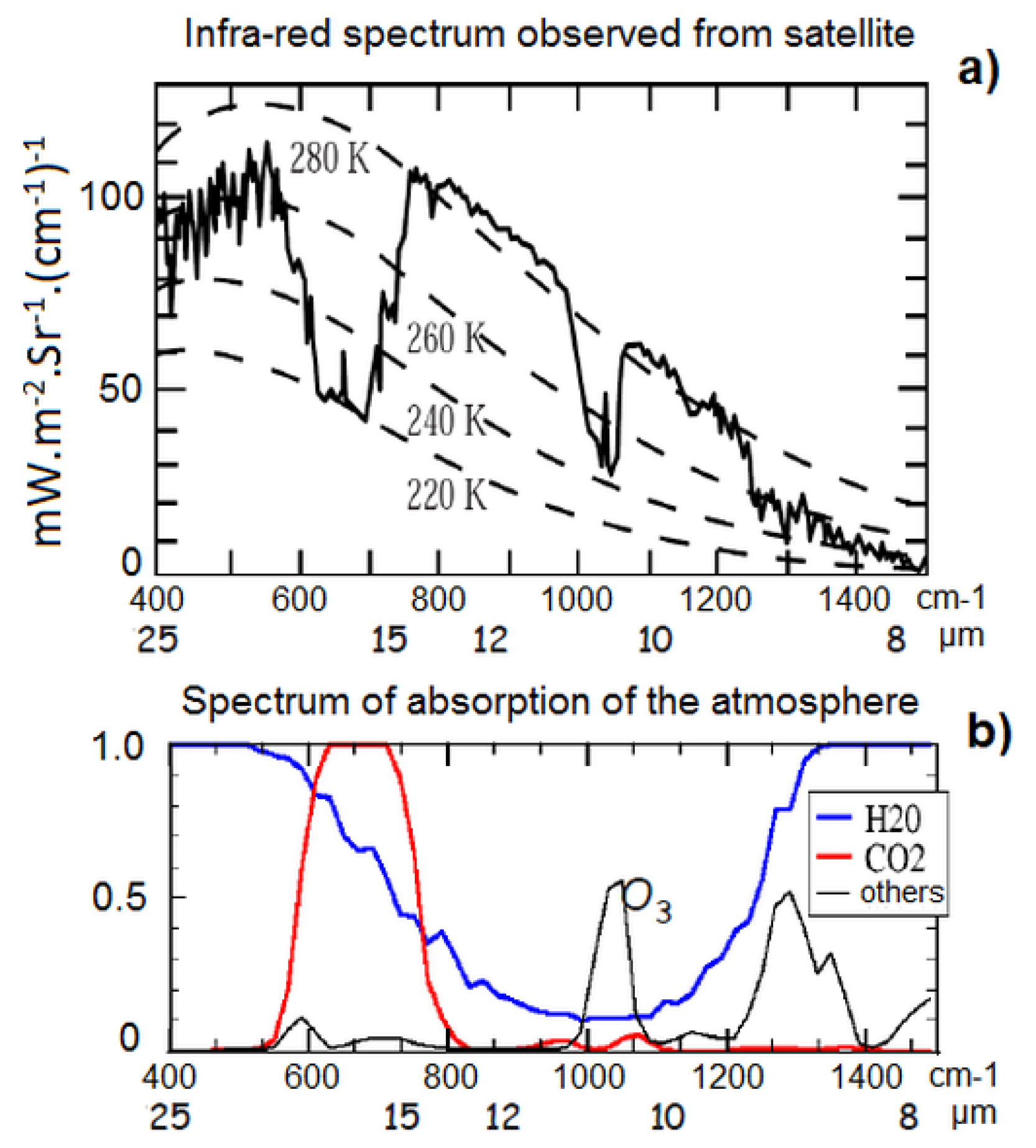
As highlighted by the Nimbus Michelson interferometer experiment [5,6], emission of outgoing longwave radiation (OLR) in the saturated absorption bands of water vapor occurs from a surface whose temperature is nearly 260 K, that is, close to the altitude of 4.3 km (Appendix A). Indeed, longwave radiation emitted from the surface of the Earth in the bands is such that the optical path is much lower that the thickness of the free convection layer. So, thermal radiation scatters up to the emission level of OLR in the bands before escaping to the outer space. The emission spectrum is that of a truncated black body radiation so that the composition of the atmosphere at the emission level does not matter as well as the density of clouds, their type or composition.
The SAT response to anthropogenic forcing reflects the height variations of the emission level of OLR in the bands . Lifting the emission level height of OLR in the bands increases radiative forcing resulting from water vapor and clouds because outgoing thermal radiations escape from a cooler surface. Lowering the temperature of the emission surface increases the temperature of the atmosphere under . At mid-latitudes a 46-m lifting of generates an increase in SAT of 0.1 °C (Appendix A). Note that the level of is lower than that of which is nearly 12 km.
Depending on the latitude, a perturbation in the climate system, which results from temperature increase in the tropopause, may increase the height , which results from properties of the moist adiabat. A positive feedback occurs, leading to amplifying forcing effects. So, the varying environmental and moist adiabats throughout the Earth’s atmosphere are of critical importance to understand and model the spatial variability of the SAT response to anthropogenic forcing [7].
Representing in an idealized environmental adiabat that promotes baroclinic instabilities in the atmosphere determines if a parcel of rising air will rise high enough for its water to condense to form clouds, and, then whether the air will continue to rise. Then, deep, moist convection may ensue, as a parcel rises to the level of free convection, after which it enters the free convective layer and rises to and beyond.
Atmospheric baroclinic instabilities can lead to the formation of low-pressure systems. There is ample theoretical and observational evidence that deep, moist convection locally establishes a “moist adiabatic” temperature profile [3,8]. This adjustment happens directly at the scale of individual convective clouds, but dynamical processes extend the radius of influence of the adjustment to the mesoscale, even the synoptic scale. being tightly controlled by the moist adiabat, it is during these periods of instability that the perturbation of the Earth’s radiation balance is exerted with the concomitant increase in SAT, before the atmosphere becomes stable again.
Thermal fluxes that impact SAT in a perturbed climate system are asymmetrical depending on whether they are incoming or outgoing fluxes. Incoming fluxes warm the surface of the Earth quasi-instantaneously since the thermal energy is accumulated while the climate system is perturbed as a result of radiative forcing partially trapped under . A transient thermal equilibrium between the surface and the atmosphere occurs rapidly because of precipitations and sensible heat fluxes resulting from the low-pressure systems. On the other hand, when the atmosphere becomes stable again, the thermal exchanges that make the surface temperature tends to recover the value it should have kept if the climate system had not been perturbed are much slower. The surface–atmosphere system behaves like a quasi-isolated thermodynamic system because exchanges are mainly ruled by evaporative processes. This implies that the heat accumulated is conserved on a synoptic scale (Appendix B).
From these general considerations, the article proposes to consider the anthropogenic impact on the various climate systems of the planet in order to concretely elucidate the mechanisms involved in feedbacks. It will be shown how idealized environmental adiabats are deduced from the spatial distribution of reduced rainfall height (RRH) in two bands characteristic of annual and inter-annual variability. It will then be possible to infer the variation of in the perturbed climate system and to compare the observations of the sensitivity of the SAT response to the anthropogenic forcing at the planetary scale.
2. Data
Monthly SAT from 1856 to 2015 gridded (5° × 5°) were provided by the Climatic Research Unit [9]. Monthly SAT and SST data from 1981 to 2010 gridded (1° × 1°) were provided by the National Oceanic and Atmospheric Administration NOAA/OAR/ESRL PSD, Boulder, Colorado, USA [10]. Monthly rainfall height data from 1901 to 2009 gridded (1° × 1°) were provided by NOAA [11].
3. Method
3.1. Representation of the Surface Air Temperature (SAT) Anomalies
The anthropogenic component responsible for the surface temperature increase since 1970 was deduced from the analysis of instrumental temperatures before 1970 by fitting the variations observed from a combination of the sea surface temperature (SST) anomalies at areas relevant to the ocean [1,12]. Indeed, climate variability is closely linked to SST anomalies where long-period Rossby waves winding around the five subtropical gyres are resonantly forced by solar and orbital forcing.
SAT variations observed in the middle of the 20th century reflect the natural variability of the climate unlike the quasi-linear rise observable since 1970. The coefficients of the linear combinations of the relevant SST anomalies having been fitted before 1970, it is then possible to extract the natural variability of the climate from the instrumental SAT by extending the combination of SST anomalies to the present day. The anthropogenic component of SAT is deduced from the residual. The size of grid cells allows us to minimize the noise in the spatial pattern of the variations in temperature and to reduce the uncertainties in instrumental measurements by considering a large number of them.
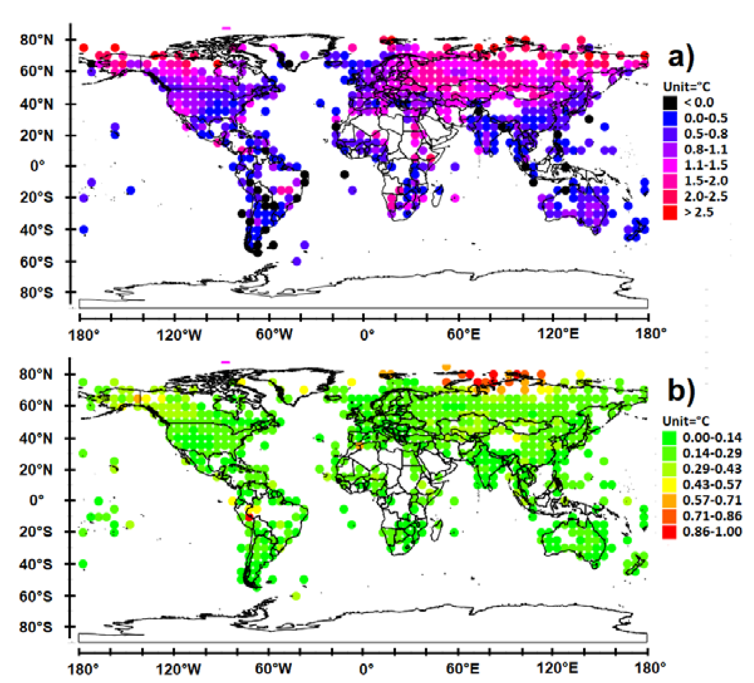
The SAT response to anthropogenic forcing shows considerable spatial disparities (Figure 1). If we exclude the anomalies observed in eastern Africa that border the Libyan Desert, the tropical band is minimally impacted, whereas anomalies increase at mid-latitudes and become very high at high latitudes in the northern hemisphere where the Arctic amplification occurs (no measurements are available in the southern hemisphere), reaching more than 2.5 °C. To this latitudinal variation is superimposed a longitudinal modulation especially perceptible at mid-latitudes. Lower than 0.8 °C and even 0.5 °C in northern Australia, southern South America, eastern North America, northern and western Europe, it overreaches 2 °C in eastern Europe, Russia, Kazakhstan, Mongolia, and west of North America, east of Brazil, southern Africa, and southern Australia.
The Earth’s response to increasing anthropogenic emissions can only find an explanation by looking for a positive feedback. Indeed, the direct impact of the induced radiative forcing (a few tenths of degrees since 1970) is very low compared to what is observed in some regions, heavily impacted by the anthropogenic warming such as the Arctic.
3.2. Representation of the Precipitations
The representation of the rainfall patterns on a planetary scale in two cycles, that is, 5–10 years and 0.5–1.5 years provides us with valuable information on the mechanisms responsible for the disparity of the observed anthropogenic response. Since the average annual rainfall height is not relevant in our analysis because it may reflect local variability while we are interested in the synoptic scale, rainfall is reduced, that is, divided by the mean rainfall height.
The method pursued in this paper relies on the wavelet analysis [13,14] of reduced rainfall height (RRH) in relevant bands in order to disentangle the relevant cycles. Wavelet analysis has become a common tool for analyzing localized variations of power within a time series. By decomposing a time series in time-frequency space, one can determine both the dominant modes of variability and how those modes vary in time. A wavelet analysis of RRH series with a spatial resolution of 0.5 degree allows representing the regions subject to oscillation phenomena when the wavelet power is scale-averaged over the relevant frequency bands.
However, the wavelet power is not enough when one seeks to specify the phase, which expresses when the oscillation reaches its extrema, with respect to a temporal reference (TR). The TR must also display an oscillation in the relevant frequency band. For example, the southern oscillation index (SOI) is used as TR in the 5–10-year band. The cross-wavelet analysis of both RRH and TR expresses the cross-wavelet power and the coherence phase. The cross-wavelet power of RRH and TR divided by the square root of the wavelet power of TR coincides with the square root of the wavelet power of RRH, that is, the amplitude of the RRH oscillation. The coherence phase of RRH and TR shows the time shift between the RRH oscillation and the TR. Thus, the spatial representation of the oscillations requires paired figures; the first is the amplitude of anomalies (regardless of the time when the anomaly reaches its maximum), and the second is the phase (the time evolution, that is, the time when the anomaly reaches its maximum over a period).
A cross-wavelet analysis is preferred to a Complex Empirical Orthogonal Function (EOF) analysis to investigate the RRH oscillations within bandwidths [15]. If the two methods are similar for typical frequency domain analyses, that is, the power spectral and coherency analyses, they are far different in terms of the time domain. In complex EOF analysis, the time lag between time series is basically the computation of eigenvector and eigenvalue of a covariance or a correlation matrix computed from a group of original time series data. In contrast, the cross-wavelet analysis is well suited to highlight the time lag between time series when it varies continuously.
3.2.1. Regions Subject to Rainfall Oscillation
RRH anomalies in the 5–10-year cycle reflect subtropical depressions and extratropical cyclones. The choice of this cycle allows getting rid of the El Niño Southern Oscillation (ENSO) because most ENSO events occur within less than 5 years of interval. At mid-latitudes this band highlights a direct oceanic influence. The oscillation of precipitation is characteristic of atmospheric baroclinic instabilities induced from Rossby waves at high latitudes of the 5 subtropical gyres: Table 1 [16]. Waters located at the SST anomalies at the antinodes of 8-year period quasi-stationary Rossby waves may cause the overlying atmosphere to be unstable enough to sustain convection and thunderstorms, supposing low amounts of wind shear. Extratropical cyclones may move to the continents. The amplitude of the anomalies generally varies a lot over time. It may weaken for a few cycles before strengthening, which requires a long time of observation. This is the reason why the cross-wavelet of RRH is time-averaged over more than one century to be representative.
In contrast, within the tropical belt all continents are subject to the rainfall oscillation in the 5–10-year cycle. SST anomalies produce quasi-geostrophic motion of the atmosphere from heating. From the heating zone are formed equatorial-trapped eastward Kelvin waves and westward Rossby waves, hence easterly trade winds set up by atmospheric Kelvin waves to the east and westerlies as an atmospheric planetary wave response to the west [17].
3.2.2. Regions Subject to Seasonal Rainfall
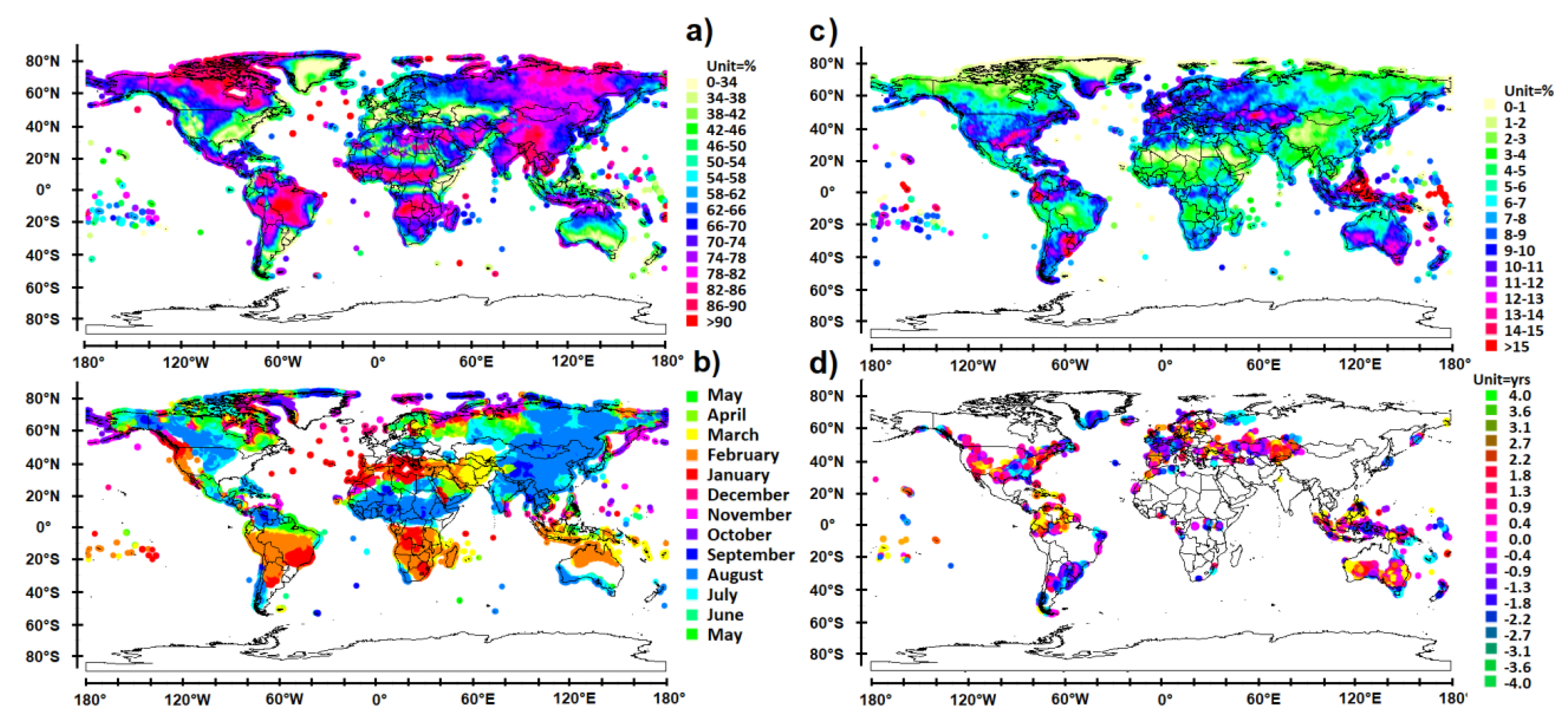
RRH anomalies in the 0.5–1.5-year cycle show a strong intra-annual variability from the annual precipitation pattern, which characterizes continental baroclinic instabilities of the atmosphere that occur in late summer most of the time (Figure 2c). The origin of low-pressure systems is multiple depending on whether concerned regions are impacted by polar vortices, low-pressure systems over large landmasses in temperate latitudes, monsoon trough, thermal lows, or tropical cyclones.
The way low-pressure systems develop from polar vortices exhibits a strong seasonality. Polar vortices result from the weakening of the northern vortex while it separates into two or more vortices [18]. They develop near Baffin Island and Canada on the one hand and northeast Siberia on the other hand (Figure 2a,c). Low-pressure systems occur in July–August in northeast Siberia, in April–May in northwestern Canada, in October–November in western Greenland, and in December–January west of the Baffin Bay. This marginal sea of the North Atlantic Ocean causes frequent storms, especially in winter, hence this anachronism.
Low-pressure systems over large landmasses in temperate latitudes occur in late summer most of the time, when the difference between temperatures aloft and SAT is greatest. They occur mostly in the northern hemisphere, where the kind of large landmasses at temperate latitudes is required for this type of lows to develop. Precipitations are concentrated mostly in the warmer months. Low-pressure systems occur in May–June in western Siberia, in July–August in eastern and far-east Siberia, in August in Mongolia and central China, in June–July in central Canada, in August in south western Canada and the central US in May–June in northern and eastern Canada, and in March–April in Quebec. Only a few areas—in the mountains of the Pacific Northwest of North America and in Iran, northern Iraq, adjacent Turkey, Afghanistan, Pakistan, central Asia, and east of the Hudson Bay—show a winter maximum in precipitation.
Elongated areas of low-pressure form at the monsoon trough or intertropical convergence zone as part of the Hadley cell circulation [19]. Monsoon troughing occurs in both hemispheres during the late summer when the wintertime surface ridge in the opposite hemisphere is the strongest. The large-scale thermal lows over the continents help create pressure gradients, which drive monsoon circulations [20]. In the northern hemisphere, monsoons occur in August in south-east Asia and eastern India, in tropical Africa, including the south of the Arabian Peninsula, and in central and northern South America. In the southern hemisphere, monsoons occur in February in northern Australia, Indonesia, and in January–February in tropical Africa including Madagascar, and in central South America (Figure 2a,b).
Thermal lows occur during the summer over continental areas across the subtropics, such as the Sonoran Desert, the Mexican and the Tibetan plateaus, the Sahara, South America, the lee of the Rocky Mountains, and southeast Asia [21]. In deserts, lack of ground and plant moisture that would normally provide evaporative cooling can lead to intense, rapid solar heating of the lower layers of air. The hot air is less dense than the surrounding air, cooler.
Worldwide, tropical cyclone activity peaks in late summer, when the difference between temperatures aloft and SSTs is greatest.
3.2.3. Complementarity of the Two Cycles
If we exclude Saharan Africa between 20 and 30° N in which rainfall is rare and sporadic, the map of RRH scale-averaged over the relevant cycles shows complementarity of the two main rainfall patterns virtually without any overlap (only the amplitude of anomalies is considered). The regions dominated by the rainfall oscillation in the 5–10-year cycle reveal a very low intra-annual variability. On average, rainfall is evenly distributed throughout the year. On the other hand, regions characterized by a high seasonality of precipitation, which are mainly represented by vast continental areas, do not show any significant inter-annual cycle. Rainfall patterns strongly influence the Earth’s response to anthropogenic forcing the regions subject to the rainfall oscillation in the 5–10-year cycle are much less affected than those subject to a high seasonality.
4. Results and Discussion
4.1. Evolution of the Moist Adiabat
Variations of the moist adiabat throughout the Earth’s atmosphere determine if a parcel of rising air will reach to contribute to feedbacks (Appendix C). To understand the longitudinal and latitudinal responses of the Earth to the anthropogenic forcing, we have first to consider the evolution of the moist adiabat versus the temperature at the altitude z = 0. Indeed, the way to make the atmosphere unstable is based on the properties of the moist adiabat as the air rises to the level of free convection. Consider a small increase in the temperature of the atmosphere as a perturbation resulting from radiative forcing induced by increasing anthropogenic emissions. The feedback of the atmosphere to this perturbation depends on how the convective available potential energy (CAPE) increases as a result of warming. Increase in CAPE increases the difference in density between the environmental and the moist adiabats, which favors deep, moist convection, even more as CAPE is higher.
Although the parcel method and CAPE ignore the pressure perturbation [22], they can be used in the present context that focuses on slow changes in convective processes. The sensitivity of CAPE to warming results from the behavior of the moist adiabat compared to the dry adiabat (which does not depend on the temperature); the environmental adiabat is between those two adiabats above the convective condensation level when the atmosphere becomes unstable (Figure 3).
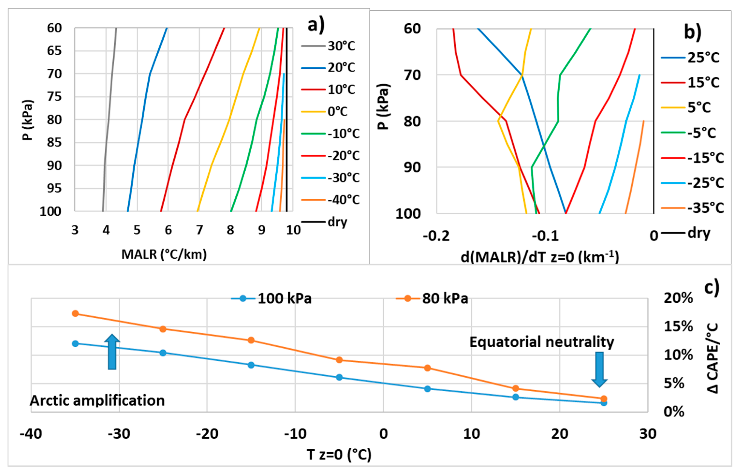
As shown in Figure 4a, the Moist Adiabatic Lapse Rate (MALR) gets closer to the dry adiabatic lapse rate as the temperature of the moist adiabat at the altitude z = 0 drops. In Figure 4b, the derivatives are always negative, whatever . This means that the dry and moist adiabatic lapse rates move away from each other as the temperature rises, and the faster the temperature increases. Consequently, for a fixed environmental adiabat, CAPE increases under the effect of increasing . So moist convection is promoted, which transiently lifts the level .
Under the effect of increasing , the climate system is potentially even more perturbed as the increase in CAPE is significant, compared to the unperturbed state. The minimum relative increase in CAPE as a function of at levels for which atmospheric pressure is 80 and 100 kPa is represented in Figure 4c. It is the ratio of the shifting of the wet adiabatic lapse rate for a 1 °C increase in over the deviation between the wet and dry adiabatic lapse rates. When is about −40 °C, the moist and dry adiabatic lapse rates are confused so that CAPE is extremely sensitive to warming of the atmosphere that separates the two adiabatic lapse rates while increases. At low temperatures, relative increase in CAPE remains close to the minimum value because the environmental adiabat is very constrained while this constitutes a lower limit at higher temperatures, the actual value depending much on the type of climate considered. The environmental adiabat is subject to a strong seasonality in the intertropical convergence zone. In winter it approaches the dry adiabat at the horse latitudes where the dry branch of the Hadley cell is descending. Therefore, instability of the atmosphere reaches its maximum, hence the moist, deep convection and the ascending branch of the Hadley cell that encircles Earth near the meteorological equator. Consequently, relative increase in CAPE that results from an increase in is very low, close to its minimum value (Figure 3a and Figure 4c).
This representation explains the strong influence of latitude on the anthropogenic forcing efficiency, which includes the Arctic amplification and the equatorial neutrality for which the positive feedback is low. Furthermore, sensitivity in CAPE to increasing grows with altitude.
For °C, the height of convection increases nearly proportionally to the temperature perturbation. Indeed, concomitantly to the increase in the energy available to convection, a rise of increases the radiative forcing because outgoing thermal radiations are reduced. So, a positive feedback loop occurs, fixing a new . For °C, the height of convection is much less sensitive to the temperature perturbation. An intermediate situation occurs when °C.
The deviation between SAT and the temperature of the moist adiabat at the altitude z = 0 depends on the altitude of the convective condensation level (Figure 3). SAT at the ground or sea level may be much higher than , especially at low latitudes where the deviation between the dry and moist adiabatic lapse rates is maximum. In contrast, at high latitudes both dry and moist adiabatic lapse rates are close so that, SAT is close to . Supposing the altitude of the convective condensation level to be 2 km, the deviation between and can be estimated by the linear relationship, using formula explicated in Appendix C:
An air parcel ascending from the near surface layer must work through the stable layer of convective inhibition when present. This work comes from sufficiently increasing instability in the low levels by rising the dew point. This is what happens in late summer over the continents, when the difference between temperatures aloft and SAT is maximum (Figure 3a).
4.2. Latitudinal Variations of SAT
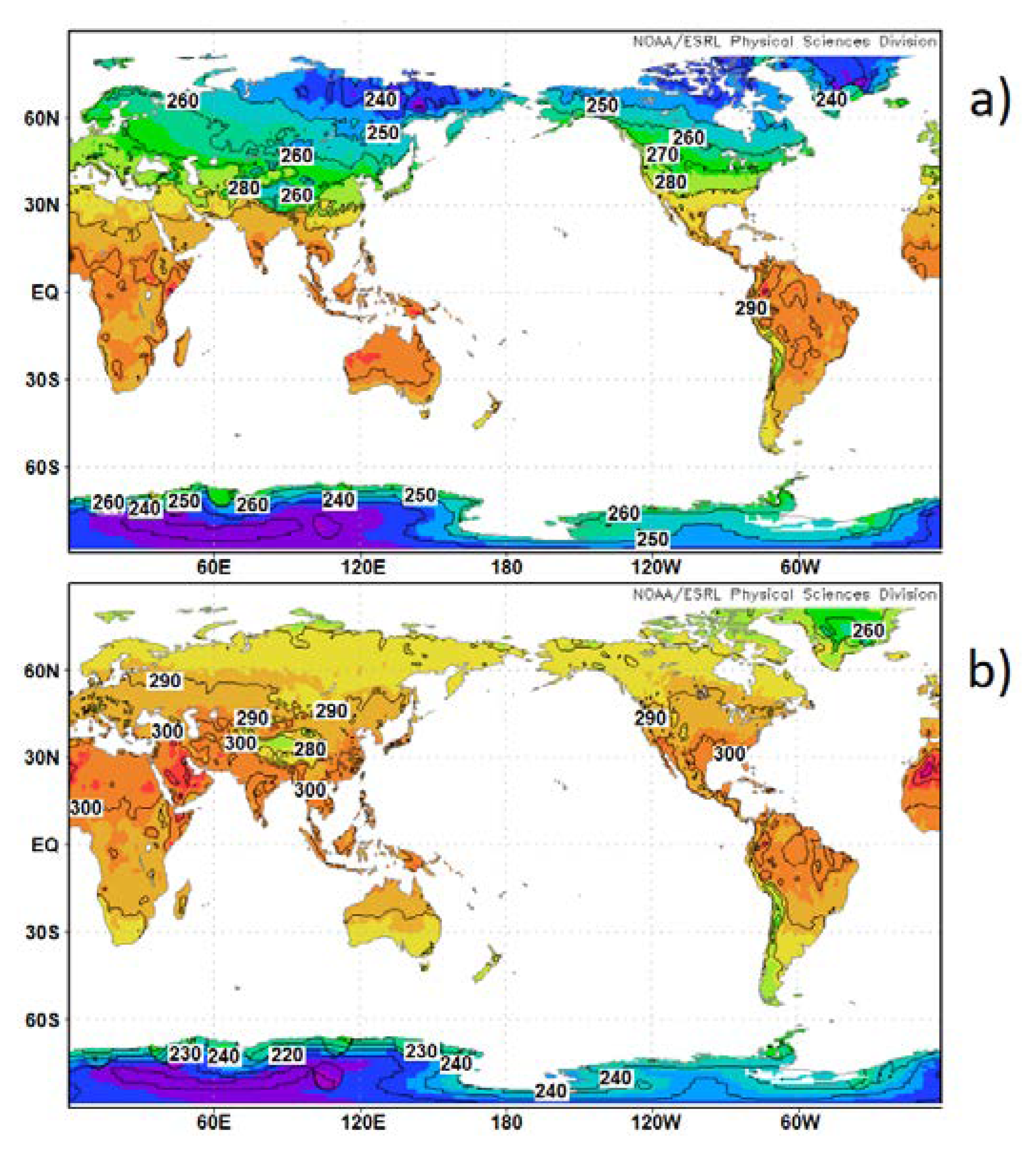
As far as the latitudinal variations of SAT resulting from the Earth’s response to anthropogenic forcing are concerned, they reach their maximum near the poles, overreaching 2.5 °C, what is commonly named the Arctic amplification. In late summer, goes down around 240 K in the Arctic, even less in the Antarctic (Figure 5): the dry and moist adiabatic lapse rates are close to each other at −30 °C. An increase in the temperature perturbation generates an increase in the moist adiabatic lapse rate so that deep, moist convection is strengthened (Figure 4). This results in lifting and the concomitant positive feedback.
Between 30° N and 60° N and between 20° S and 40° S the SAT response to anthropogenic forcing may reach 1.5 °C. In late summer, SAT goes around 290 K, i.e., .
Between 30° N and 20° S the SAT response to anthropogenic forcing is generally lower than 0.5 °C, even negative. In late summer, SAT goes around 300 K, i.e., .
4.3. Longitudinal Variations of SAT
The longitudinal variation of the SAT response to anthropogenic forcing is imputable to the oceanic influence that results from atmospheric baroclinic instabilities induced from Rossby waves at high latitudes of the subtropical gyres, nearly 40° N in the North Atlantic and the North Pacific, 40° S in the South Pacific, and 30° S in the South Atlantic and the South Indian Ocean. Unlike continental areas, no seasonal instability occurs here but inter-annual cycles are observed in connection with the SST anomalies. Oceanic baroclinic instabilities no longer result from a change in the environmental adiabat. Here, the thermal anomaly of the surface of the ocean enhances evaporative processes, which lowers the level of free convection (Figure 3b). Consequently, CAPE is much lower than that of continental areas in late summer.
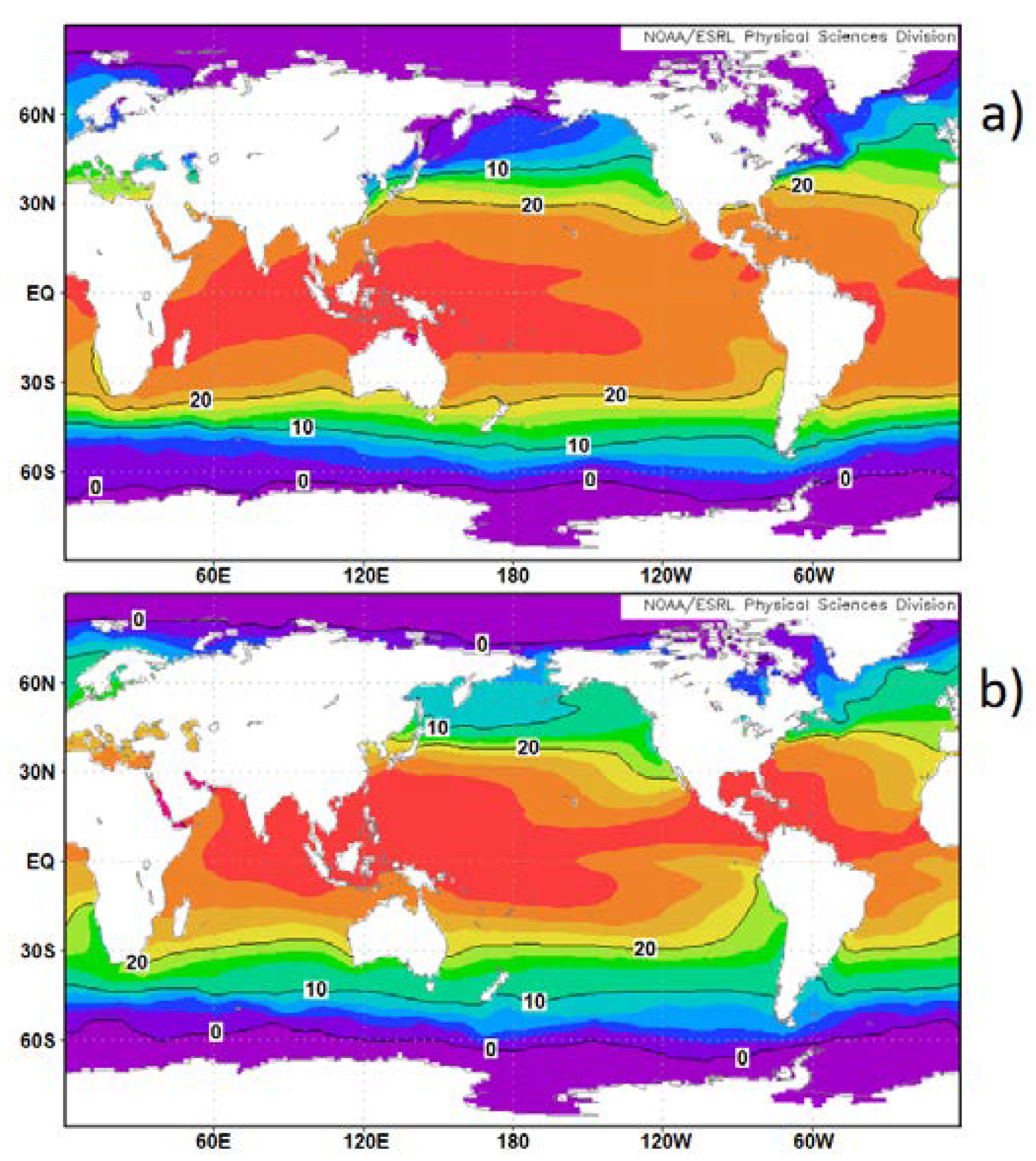
SST is between 15 and 20 °C along the year, in both hemispheres (Figure 6). Supposing a thermal equilibrium at the interface ocean-atmosphere, is around 8–12 °C from (1). Consequently is only slightly shifted in the perturbed state (Figure 4). So, the SAT response to the temperature perturbation is low, as well.
4.4. Anthropogenic Forcing Efficiency
The mode of low-pressure system formation varies a lot on planet scales; therefore, the various climate systems are differently impacted by the anthropogenic forcing. The anthropogenic forcing efficiency reflects the amplitude of the SAT response to anthropogenic forcing as a function of longitude and latitude.
4.4.1. Seasonal Low-Pressure Systems
- The low SAT of regions most impacted by polar vortices are subject to a very high sensitivity to anthropogenic forcing > 2.0 °C/50 years from Figure 1 ( is increase in SAT resulting from the anthropogenic forcing).
- Large landmasses in temperate latitudes are significantly affected by anthropogenic forcing 1.1 °C/50 years < < 2.0 °C/50 years.
- The impact of anthropogenic forcing in the monsoon trough or the intertropical convergence zone is low within the tropical belt but increases significantly as the latitude increases as occurs in South America and central Africa, up to 35° S. It is −0.5 °C/50 years < < 0.8 °C/50 years within the tropical belt and 0.8 °C/50 years < < 1.5 °C/50 years at higher latitudes.
- Regions concerned by thermal lows are heavily impacted by anthropogenic forcing because in such dry regions the convective condensation level is elevated several kilometers so that the difference between SAT and may reach up to 35 °C. Consequently 1.1 °C/50 years < < 2.0 °C/50 years.
- Regions impacted by tropical cyclones are also affected by monsoon troughing so that the anthropogenic impact is the same in both cases −0.5 °C/50 years < < 0.8 °C/50 years within the tropical belt.
4.4.2. Subtropical Depressions and Extratropical Cyclones
These are initiated in high latitudes of the five subtropical gyres at the antinodes of quasi-stationary Rossby waves [16]. The main impacted areas are (Table 1): (a) southwestern North America; (b) Texas; (c) southeastern North America; (d) northeastern North America; (e) southern Greenland; (f) Europe and central and western Asia; (g) the region of the Río de la Plata; (h) southwestern and southeastern Australia, and (i) southeastern Asia. Each region is associated with an SST anomaly. Extratropical cyclones can occur all year long. They are initiated by baroclinic instabilities of the atmosphere, then they are developed as waves along weather fronts before occluding as cold-core cyclones. However, they may be subject to moderate annual variability like UK and Netherlands where they are formed each winter. As previously seen the anthropogenic impact on the regions concerned is relatively low −0.5 °C/50 years < < 0.8 °C/50 years except when several precipitation patterns are superimposed as occurs in western Europe.
The narrow strip along the equator between 10° N and 10° S is subject to quasi-geostrophic motion of the atmosphere from heating resulting from SST anomalies whose periodicity is plurennial. The main driver is ENSO and, therefore, all concerned continents are impacted, that is, the north of south America, equatorial Africa, and Indonesia. These regions are warm all year long so that they are minimally impacted by the anthropogenic forcing −0.5 °C/50 years < < 0.8 °C/50 years.
4.4.3. The Case of the Antarctic
A problem is pending regarding the behavior of the Antarctic, which differs from that of the Arctic. Although the Antarctic is colder than the Arctic, as shown in Figure 5, the former warms less quickly than the latter, which contradicts what has been exposed previously. This suggests that, in the Antarctic, most of the time the convective condensation level is high enough to prevent any moist convective process from occurring so that properties of the moist adiabat do not apply here.
5. Conclusions
The purpose of this article was to explore simply, from well-established physical principles, what underlies the amplifying effects acting on the anthropogenic climate forcing that varies considerably at different latitudes and longitudes. A straightforward mechanism was proposed, aiming at controlling the amplitude of the SAT response to anthropogenic forcing according to the various local climate systems. To do this, idealized environmental adiabats were deduced from the precipitation patterns at planetary scale. Intended to construe how both seasonal low-pressure systems and subtropical depressions develop, they allow explaining the latitudinal and longitudinal variations in the amplitude of the observed SAT response to anthropogenic forcing.
The approach was based on the properties of the moist adiabat as a function of the temperature at z = 0. The emission level height responds to a small temperature perturbation of the atmosphere in accordance with . In return, a vertical motion of induces a variation of . When rises, the temperature of the thermal radiations emitted from the corresponding level of the atmosphere lowers, which induces an increase in the temperature of the atmosphere below that level. So, a powerful positive feedback loop occurs, leading to amplifying forcing effects. It is the reason why the climate response strongly depends on latitude. Another consequence is that, for a given latitude, the response of to anthropogenic forcing differs according to whether atmospheric instabilities have a continental or oceanic origin, depending on the value of itself.
The actual SAT varies in the same direction as , the deviation between these two variables depending on the altitude of the convective condensation layer. The latter strongly depends on the local climate system so that the maximum deviation is observed over desert regions. Besides, at high latitudes the positive feedback reacts synergistically with the reduction of albedo due to melting of the ice in summer.
To summarize, the spatial distribution of the observed SAT response to anthropogenic forcing can be construed by emphasizing the key role of the moist adiabat, depending on the various climate systems. The response of temperature to the perturbation is fast, whereas the return to its initial state before the development of the cyclonic system is very slow, while the perturbed climate system behaves like a quasi-isolated thermodynamic system. So, the SAT response to anthropogenic forcing turns out to be the result of a succession of events with asymmetrical surface–atmosphere heat exchanges where low-pressure systems occur.
Funding
This research received no external funding.
Acknowledgments
May the two anonymous reviewers be generously thanked for the considerable work they have done in improving the readability and understanding of the document, as well as for their patience.
Conflicts of Interest
The authors declare no conflict of interest.
Appendix A. Radiative Forcing Efficiency
At thermal equilibrium, the solar energy received by the Earth is equal to the thermal energy re-emitted into space as infrared radiation. By writing that the infrared flux emitted = solar flux absorbed, we obtain the well-known relationship:
where 4πR2 represents the surface of the Earth, σTe4 the emission of black body, (1 − A) the absorption coefficient, πR2 the Earth equatorial section, F0 the extraterrestrial solar flux; Te is the radiative equilibrium temperature, A the planetary albedo, and σ the Stefan-Boltzmann constant (5.67.10 −8 W.m−2.K −4).
4πR2σTe4 = (1 − A) πR2F0
The emitted radiative power σTe4 balances the incident radiative power of solar shortwave radiation reaching the surface of the Earth (1 − A)F0/4, i.e., 240 W/m2 (F0 = 1365.8 W/m2 [23], the current albedo is close to 0.3), which gives Te = −18 °C (255 K).
The mean global temperature of the Earth is 15 °C (288 K), which corresponds to a radiative power equal to σTe4 = 390 W/m2. The difference between this radiative power and what would be emitted in the absence of atmosphere is 390 − 240 = 150 W/m2, corresponding to the absorption by the real atmosphere in the presence of water vapor, greenhouse gases, clouds, and aerosols. The radiative forcing efficiency is then (288 − 255)/150 = 0.22 °C/(W/m2).
Figure A1.
(a) Longwave spectra of the atmosphere from Nimbus Michelson interferometer – (b) Longwave spectra from the HITRAN2012 molecular spectroscopic database [24].
Figure A1.
(a) Longwave spectra of the atmosphere from Nimbus Michelson interferometer – (b) Longwave spectra from the HITRAN2012 molecular spectroscopic database [24].

The wavelengths of saturated absorption bands of water vapor lie between 5 and 8 µm and above 18 µm or in wavenumbers between 1250 and 2000 cm−1 and under 550 cm−1. By integrating the black body emission spectrum at the temperature of 260 K over the bands (Figure A1), the outgoing radiation energy in is 126 W/m2: 46% of the total energy of longwave radiation is emitted in considering that the latter extends to small wavenumbers. The decrease in the energy of the outgoing thermal radiation as the temperature at decreases by 1 K is 1.52 W/m2. Supposing the temperature gradient versus altitude is −6.5 °C/km, and using the radiative forcing efficiency, SAT increases by 0.1 °C when rises 46 meters ( is 4.3 km high at mid-latitudes if a mean SAT of 15 °C is considered).
Appendix B. The Differential Fluxes Resulting from the SAT Anomaly
Outgoing heat fluxes from the surface are the differential fluxes resulting from the positive SAT anomaly ΔT. Those differential fluxes are threefold: the radiative flux , the latent heat flux , and the sensible heat flux . Knowing the radiative flux , the latent heat flux , and the sensible heat flux , the differential fluxes are calculated so that [25].
Radiation Heat Transfer
Radiation heat transfer is ruled by the Stefan-Boltzmann Law, that is, the radiation energy per unit time and per square meter from a black body is proportional to the fourth power of the absolute temperature where is the heat transfer per unit time and per square meter (W), σ is the Stefan-Boltzmann constant and is the absolute temperature. The net surface thermal radiation resulting from the surface temperature anomaly is therefore .
Latent Heat Flux
The latent heat flux results from the evaporation of the surface which depends on the average specific humidity : where is the latent heat of vaporization equal to 2.5 × 10⁶ J/kg, and the mean vertical wind component, in m/s [17]. The specific humidity of the air is expressed as a function of the temperature in °C:
The latent heat flux resulting from the surface temperature anomaly is . Since then and .
Sensible Heat Flux
The sensible heat flux results from the transfer of heat by convection from the surface to the atmosphere. The convection equation may be expressed as: where ρ is the density of the air, the specific heat capacity of air, the temperature of the surface and the temperature of the atmosphere. The net sensible differential heat flux resulting from the surface temperature anomaly is the product of the net sensible heat flux at the considered location multiplied by its relative variation due to the thermal anomaly. Therefore, .
As shown in Table A1, the latent heat flux is by far the largest since it is −0.46 W/m2 at mid-latitudes, whereas the radiative flux is −0.09 W/m2: this outgoing flux is negligible in comparison to the quasi-conservative flux W/m2.

Table A1.
Expression of the mean heat fluxes resulting from the SAT anomaly ΔT at mid-latitudes. is the outgoing radiation flux, the latent heat flux, the sensible heat flux, from “European Reanalysis ERA40” [26]. The differential fluxes , , and are induced by the SAT anomaly. The sensible heat flux is approximate. SAT and ΔT are indicative since they are intended for the comparative study of ingoing and outgoing fluxes.
| SAT °C | ΔT °C | ||||||
|---|---|---|---|---|---|---|---|
| 12 | 0.14 | −45 | −0.09 | −50 | −0.46 | −15 | −0.30 |
Appendix C. The Moist Adiabatic Lapse Rate Versus Temperature
The formula for the moist adiabatic lapse rate is given approximately by in the following [27]:
where:
- wet adiabatic lapse rate, K/mEarth’s gravitational acceleration = 9.8076 m/s2heat of vaporization of water = 2501000 J/kgspecific gas constant of dry air = 287 J/kg·Kspecific gas constant of water vapor = 461.5 J/kg·Kthe dimensionless ratio of the specific gas constant of dry air to the specific gas constant for water vapor = 0.622the water vapor pressure of the saturated air
The August-Roche-Magnus equation, as described in [28] provides the coefficients used here:
- ; is the temperature of the saturated air in °Cthe mixing ratio of the mass of water vapor to the mass of dry air [29]the pressure of the saturated airtemperature of the saturated air, Kthe specific heat of dry air at constant pressure, = 1003.5 J/kg·K
The moist adiabat at the altitude is represented in an emagram [30].
References
- Pinault, J.-L. Anthropogenic and natural radiative forcing: Positive feedbacks. J. Mar. Sci. Eng. 2018, 6, 146. [Google Scholar] [CrossRef] [Green Version]
- Stephens, G.L. Cloud feedbacks in the climate system: A critical review. J. Clim. 2005. [Google Scholar] [CrossRef] [Green Version]
- Stocker, T.F.; Clarke, G.K.C.; Treut, H.L.; Lindzen, R.S.; Meleshko, V.P.; Mugara, P.K.; Palmer, T.N.; Pierrehumbert, R.T.; Sellers, P.J.; Trenberth, K.E.; et al. Physical climate processes and feedbacks. In Climate Change 2001: The Scientific Basis, Contributions of Working Group I to the Third Assessment Report of the Intergovernmental Panel on Climate Change; Houghton, J.T., Ed.; Cambridge University Press: Cambridge, UK, 2001. [Google Scholar]
- Benestad, R.E. A mental picture of the greenhouse effect. Theor. Appl. Climatol. 2017, 128, 679–688. [Google Scholar] [CrossRef] [Green Version]
- Hanel, R.A.; Schlachman, B.; Rogers, D.; Vanous, D. The Nimbus 4 Michelson interferometer. Appl. Opt. 1971, 10, 1376–1382. [Google Scholar] [CrossRef] [PubMed]
- Kyle, H.L.; Hickey, J.R.; Ardanuy, P.E.; Jacobwitz, H.; Arking, A.; Campbell, G.G.; House, F.B.; Maschhoff, R.; Smith, G.L.; Stowe, L.L.; et al. The nimbus earth radiation budget (ERB) experiment: 1975 to 1992. 1993. [Google Scholar] [CrossRef]
- Taylor, P.C.; Ellingson, R.G.; Cai, M. Seasonal variations of climate feedbacks in the NCAR CCSM3. J. Clim. 2011, 24, 3433–3444. [Google Scholar] [CrossRef]
- Betts, A.K. Saturation point analysis of moist convective overturning. J. Atm. Sci. 1982, 39, 1484–1505. [Google Scholar] [CrossRef] [Green Version]
- Jones, P.D.; Lister, D.H.; Osborn, T.J.; Harpham, C.; Salmon, M.; Morice, C.P. Hemispheric and large-scale land surface air temperature variations: An extensive revision and an update to 2010. J. Geophys. Res. 2012, 117, D05127. Available online: www.metoffice.gov.uk/hadobs/crutem4/data/ (accessed on 13 March 2020). [CrossRef] [Green Version]
- National Oceanic and Atmospheric Administration, Earth System Research Laboratory, Physical Sciences Division. Available online: https://www.esrl.noaa.gov/psd/ (accessed on 13 March 2020).
- National Oceanic and Atmospheric Administration. Available online: ftp://ftp.cpc.ncep.noaa.gov/precip/cmap/monthly/ (accessed on 13 March 2020).
- Pinault, J.-L. Resonantly forced Baroclinic waves in the oceans: Subharmonic modes. J. Mar. Sci. Eng. 2018, 6, 78. [Google Scholar] [CrossRef] [Green Version]
- Torrence, C.; Compo, G.P. A practical guide for wavelet analysis. Bull. Am. Meteorol. Soc. 1998, 79, 61–78. [Google Scholar] [CrossRef] [Green Version]
- Pinault, J.L. Global warming and rainfall oscillation in the 5–10 yr band in Western Europe and Eastern North America. Clim. Chang. 2012, 114, 621–650. [Google Scholar] [CrossRef]
- Gamage, N.; Blumen, W. Comparative analysis of low-level cold fronts: Wavelet, Fourier, and empirical orthogonal function decompositions. Mon. Weather Rev. 1993, 121, 2867–2878. [Google Scholar] [CrossRef] [Green Version]
- Pinault, J.-L. Regions subject to rainfall oscillation in the 5–10 year band. Climate 2018, 6, 2. [Google Scholar] [CrossRef] [Green Version]
- Gill, A.E. Atmosphere–Ocean Dynamics; International Geophysics Series, 30; Academic Press: Cambridge, MA, USA, 1982; p. 662. [Google Scholar]
- Polar Vortex. Glossary of Meteorology. American Meteorological Society. Available online: http://glossary.ametsoc.org/wiki/Polar_vortex (accessed on 13 March 2020).
- Intertropical Convergence Zone, Wikipedia. Available online: https://en.wikipedia.org/wiki/Intertropical_Convergence_Zone (accessed on 13 March 2020).
- Davis, M.E.; Thompson, L.G.; Yao, T.; Wang, N. Forcing of the Asian monsoon on the Tibetan Plateau: Evidence from high-resolution ice core and tropical coral records. J. Geophys. Res. 2005, 110. [Google Scholar] [CrossRef] [Green Version]
- Thermal Low. Glossary of Meteor. Available online: http://glossary.ametsoc.org/wiki/Thermal_low (accessed on 13 March 2020).
- Sun, W.-Y.; Sun, O.M. Revisiting the parcel method and CAPE. Dyn. Atmos. Ocean. 2019, 86, 134–152. [Google Scholar] [CrossRef]
- Total Solar Irradiance (TSI). Available online: https://www.ngdc.noaa.gov/stp/solar/solarirrad.html (accessed on 13 March 2020).
- Rothman, L.S.; Gordon, I.E.; Babikov, Y.; Barbe, A.; Benner, D.C.; Bernath, P.F.; Birk, M.; Bizzocchi, L.; Boudon, V.; Brown, L.R. The HITRAN2012 molecular spectroscopic database. J. Quant. Spectrosc. Radiat. Transf. 2013, 130, 4–50. [Google Scholar] [CrossRef]
- Pinault, J.-L. Modulated response of subtropical gyres: Positive feedback loop, subharmonic modes, resonant solar and orbital forcing. J. Mar. Sci. Eng. 2018, 6, 107. [Google Scholar] [CrossRef] [Green Version]
- Kallberg, P.; Berrisford, P.; Hoskins, B.; Simmons, A.; Uppala, S.; Lamy-Thepaut, S. Atlas of the Atmospheric General Circulation. ECMWF ERA-40 Project Report Series, No. 19; European Centre for Medium-Range Weather Forecasts: Shinfield, Reading, UK. Available online: http://www.ecmwf.int/publications (accessed on 13 March 2020).
- Saturation Adiabatic Lapse Rate. Glossary of Meteorology. American Meteorological Society. Available online: http://glossary.ametsoc.org/wiki/Saturation-adiabatic_lapse_rate (accessed on 13 March 2020).
- Alduchov, O.A.; Eskridge, R.E. Improved Magnus form approximation of saturation vapor pressure. J. Appl. Meteorol. 1996, 35, 601–609. [Google Scholar] [CrossRef]
- Mixing Ratio. Glossary of Meteorology. American Meteorological Society. Available online: http://glossary.ametsoc.org/wiki/Mixing_ratio (accessed on 13 March 2020).
- Emagram, Wikipedia. Available online: https://en.wikipedia.org/wiki/Emagram (accessed on 13 March 2020).
Figure 1.
(a) The increase from 1970 in the surface air temperature (SAT) responses to anthropogenic forcing observed in 2015. (b) The standard deviation.
Figure 1.
(a) The increase from 1970 in the surface air temperature (SAT) responses to anthropogenic forcing observed in 2015. (b) The standard deviation.

Figure 2.
Cross-wavelet power (a,b) and coherence phase (c,d) of reduced rainfall height (RRH), time-averaged over 1901–2009, scale-averaged over the 0.5–1.5-year cycle in a, c) and over the 5–10-year cycle in (b,d).
Figure 2.
Cross-wavelet power (a,b) and coherence phase (c,d) of reduced rainfall height (RRH), time-averaged over 1901–2009, scale-averaged over the 0.5–1.5-year cycle in a, c) and over the 5–10-year cycle in (b,d).

Figure 3.
Idealized adiabats (a) over continental regions in mid-summer (in black) and in late summer (in red). (b) above a positive sea surface temperature (SST) anomaly (in red) and above the surrounding ocean (in black) - = surface air temperature, SST= sea surface temperature, is the moist adiabat at altitude z = 0, = SST anomaly (supposing a thermal equilibrium at the interface ocean-atmosphere), CCL = convective condensation level, LFC = level of free convection, = emission level height of outgoing longwave radiation in the saturated absorption bands of water vapor, CIN = convective inhibition, CAPE = convective available potential energy—the path of a rising air parcel is in green.

Figure 4.
(a) MALR for various temperatures . The dry adiabatic lapse rate is also represented. (b) The derivative of the MALR with respect to . (c) Minimum increase in the differential of CAPE at two altitudes, which results from a 1 °C increase in .
Figure 4.
(a) MALR for various temperatures . The dry adiabatic lapse rate is also represented. (b) The derivative of the MALR with respect to . (c) Minimum increase in the differential of CAPE at two altitudes, which results from a 1 °C increase in .

Figure 5.
Monthly SAT (K) time-averaged over 1981-2010 in February (a) and August (b). These are the months for which temperatures are extreme in each of the hemispheres. (Maps provided by NOAA).
Figure 5.
Monthly SAT (K) time-averaged over 1981-2010 in February (a) and August (b). These are the months for which temperatures are extreme in each of the hemispheres. (Maps provided by NOAA).

Figure 6.
Monthly SST (°C) time-averaged over 1981-2010, in January (a) and July (b). Like in Figure 5 these are the months for which temperatures are extreme in each of the hemispheres (Maps provided by NOAA).
Figure 6.
Monthly SST (°C) time-averaged over 1981-2010, in January (a) and July (b). Like in Figure 5 these are the months for which temperatures are extreme in each of the hemispheres (Maps provided by NOAA).

Table 1.
The association of reduced rainfall height (RRH) and sea surface temperature (SST) anomalies at mid-latitudes from [16].
Table 1.
The association of reduced rainfall height (RRH) and sea surface temperature (SST) anomalies at mid-latitudes from [16].
| Location of RRH Anomalies | Location of Related SST Anomalies |
|---|---|
| Southwestern North America | eastern antinode of the North Pacific extending along the western coast of the North America between 40° N and 60° N |
| Texas | along the subtropical gyre from the Baja California peninsula between 20° N and 30° N |
| Southeastern North America, Northeastern North America, southern tip of Greenland, Europe and Western-Central Asia | western antinode of the North Atlantic subtropical gyre that follows the North American coast from the Cape Hatteras to Newfoundland around 40° N. About the southeastern North America, the SST anomaly promotes the motion of tropical cyclones from the Gulf of Mexico or the Caribbean Sea. |
| Region of the Rio de la Plata | western antinode of the South Atlantic subtropical gyre nearly 30° S |
| South-Western and South-Eastern Australia | between 90° E and the western coast of Australia, and between 20° S and 40° S in latitude |
| Southeast Asia | Like what occurs in southeastern North America, here northeastward migration of tropical cyclones is related to SST anomalies in the Northwestern Pacific |
© 2020 by the author. Licensee MDPI, Basel, Switzerland. This article is an open access article distributed under the terms and conditions of the Creative Commons Attribution (CC BY) license (http://creativecommons.org/licenses/by/4.0/).
Share and Cite
MDPI and ACS Style
Pinault, J.-L. The Moist Adiabat, Key of the Climate Response to Anthropogenic Forcing. Climate 2020, 8, 45. https://0-doi-org.brum.beds.ac.uk/10.3390/cli8030045
AMA Style
Pinault J-L. The Moist Adiabat, Key of the Climate Response to Anthropogenic Forcing. Climate. 2020; 8(3):45. https://0-doi-org.brum.beds.ac.uk/10.3390/cli8030045
Chicago/Turabian StylePinault, Jean-Louis. 2020. "The Moist Adiabat, Key of the Climate Response to Anthropogenic Forcing" Climate 8, no. 3: 45. https://0-doi-org.brum.beds.ac.uk/10.3390/cli8030045
Note that from the first issue of 2016, this journal uses article numbers instead of page numbers. See further details here.