Prediction of Autumn Precipitation over the Middle and Lower Reaches of the Yangtze River Basin Based on Climate Indices

Abstract

Autumn precipitation (AP) has important impacts on agricultural production, water conservation, and water transportation in the middle and lower reaches of the Yangtze River Basin (MLYRB; 25°–35° N and 105°–122° E). We obtain the main empirical orthogonal function (EOF) modes of the interannual variation in AP based on daily precipitation data from 97 stations throughout the MLYRB during 1980–2015. The results show that the first leading EOF mode accounts for 30.83% of the total variation. The spatial pattern shows uniform change over the whole region. The variance contribution of the second mode is 16.13%, and its spatial distribution function shows a north-south phase inversion. Based on previous research and the physical considerations discussed herein, we include 13 climate indices to reveal the major predictors. To obtain an acceptable prediction performance, we comprehensively rank the climate indices, which are sorted according to the values of the new standardized algorithm of information flow (NIF, a causality-based approach) and correlation coefficient (a traditional climate diagnostic tool). Finally, Tropical Indian Ocean Dipole (TIOD), Arctic Oscillation (AO), and other four indicators are chosen as the final predictors affecting the first mode of AP over the MLYRB; NINO3.4 SSTA (NINO3.4), Atlantic-European Circulation E Pattern (AECE), and other four indicators are the major predictors for the second mode. In the final prediction experiment, considering the time series prediction of principal components (PCs) to be a small-sample problem, the Bayesian linear regression (BLR) model is used for the prediction. The experimental results reveal that the BLR model can effectively capture the time series trends of the first two modes (the correlation coefficients are greater than 0.5), and the overall performance is significantly better than that of the multiple linear regression (MLR) model. The prediction factors and precipitation prediction results identified in this study can be referenced to rapidly obtain climatological information for AP over the MLYRB and improve the regional prediction of AP elsewhere, which will also help policymakers prepare appropriate adaptation and mitigation measures for future climate change.

1. Introduction

Over the past few years, changing precipitation patterns have been linked to climate change and attracted worldwide attention [1,2,3,4]. Studies have shown that extreme precipitation events have increased over many regions around the world, altering the hydrological cycle, ecological environment, and different society activities, such as agriculture and hydropower generation [5,6,7,8,9,10,11]. Even worse, according to numerical model simulations, these trends may continue into the next century [12]. For example, an analysis based on global-scale observation datasets shows that extreme precipitation has expanded significantly over many mid-latitude regions of the Northern Hemisphere and that areas affected by drought or severe drought have increased since the 1970s [13,14,15]. Therefore, it is important to analyze and predict changes in at different temporal and spatial scales around the world. Villarini et al. showed that increasing trends of heavy rainfall in the northern part of the central United States were related to expanded atmospheric moisture content due to rising temperatures [16]. Related research found no significant trends in annual precipitation from 1956 to 2013 over mainland China, but regional differences were noted. For instance, reduced precipitation was observed mainly in central, southeastern, southwestern and northeastern China, whereas increased precipitation was detected mainly in the middle and lower reaches of the Yangtze River Basin (MLYRB), the southeast coastal region, the Qinghai-Tibet Plateau, and northwestern China; at the same time, frequencies of extreme precipitation events in these regions have also increased significantly [17,18,19]. Studies have shown that the amount, intensity, and duration of extreme rainfall events in the MLYRB have all changed since the 1980s [17].

To improve the quality of predicting regional extreme precipitation events, it is necessary to evaluate the mechanisms responsible for these precipitation changes. Among the different aspects of these mechanisms, the influences of large-scale circulation modes, which have strong impacts on extreme precipitation events, are particularly important [20,21]. Cayan et al. suggested that the frequency distribution of daily precipitation in winter over the western United States shows a strong and systematic response to the EI Niño-Southern Oscillation (ENSO) phases [22]. Ning and Bradley also found that the ENSO phases have different influences on winter extreme precipitation events over the northeastern United States [23]. In China, many studies have pointed out that abnormal changes in precipitation are often affected by sea surface temperature (SST) anomalies. For example, the influence of ENSO on autumn precipitation (AP) is more significant than that in summer; during an El Niño year, the AP usually appears reduced over North China and intensified in southern regions [24]. In addition, during ENSO’s decaying years, its impacts on China’s climate have been promoted by the “capacitor effect” of the Indian Ocean SST [25]. Related studies have shown that the Tropical Indian Ocean Dipole (TIOD) negative phase contributes to strengthening of the Indo-Burma trough in autumn, which further promotes the transport of water vapor to the Indian Ocean and South China Sea [25,26]. Complex sea–air interactions can also affect AP in the Yangtze River Basin during autumn [27], for instance, the curvature of the summer Kuroshio Current axis, which is accompanied by large cold water masses in southern Japan. Correlation analysis has been extensively employed to assess the relationships between atmospheric circulation variability patterns and precipitation anomalies in China over the past 100 years [28]. The Southern Oscillation (SO), North Pacific Oscillation (NPO), and 500 hPa atmospheric circulation W pattern (AECW) are some examples of atmospheric circulation variability affecting mid-latitude and tropical weather conditions, including China precipitation [28]. Moreover, AP can be modulated by other low-frequency oscillations, such as the quasi-biennial oscillation (QBO) of the tropical stratosphere [29].

Although relevant research has revealed important relationships between different modes of climate variability and AP variations in China [25,26,27,28,29], the causal associations are still not fully understood. Furthermore, previous studies have focused on national or individual administrative divisions. In this study, we emphasize that there is more scientific and application value if assessing precipitation observations according to geographical characteristics. When examining the mechanisms modulating the large-scale circulation modes and related precipitation variability, physics-based regression modelling has been proposed to predict future precipitation events and effectively adopted to study summer precipitation forecasts in India, East Asia, and the MLYRB [30,31,32,33,34]. However, few related studies have used such methods to explore spatiotemporal changes in AP over the MLYRB or employed related models for quantitative predictions [34]. The MLYRB is not only a major agricultural base in China but also an area with strong societal and economic development [34]. Autumn is the season in which the East Asian summer circulation transitions to the winter circulation [35]. Many unstable factors may induce disasters, such as droughts, floods, and low temperatures [36]. Therefore, it is not only important to analyze the major drivers affecting AP over the MLYRB, but equally relevant to investigate the feasibility of predicting precipitation with an appropriate regression model. In this study, we analyze the spatiotemporal variations of AP over the MLYRB from 1980 to 2015. The information flow detection method is employed to extract potential preceding predictors and compared to time-lagged correlation analysis to assess the usefulness of the information flow algorithm. Finally, the Bayesian linear regression (BLR) model is used to predict AP over the MLYRB.

2. Data and Methodology

2.1. Data

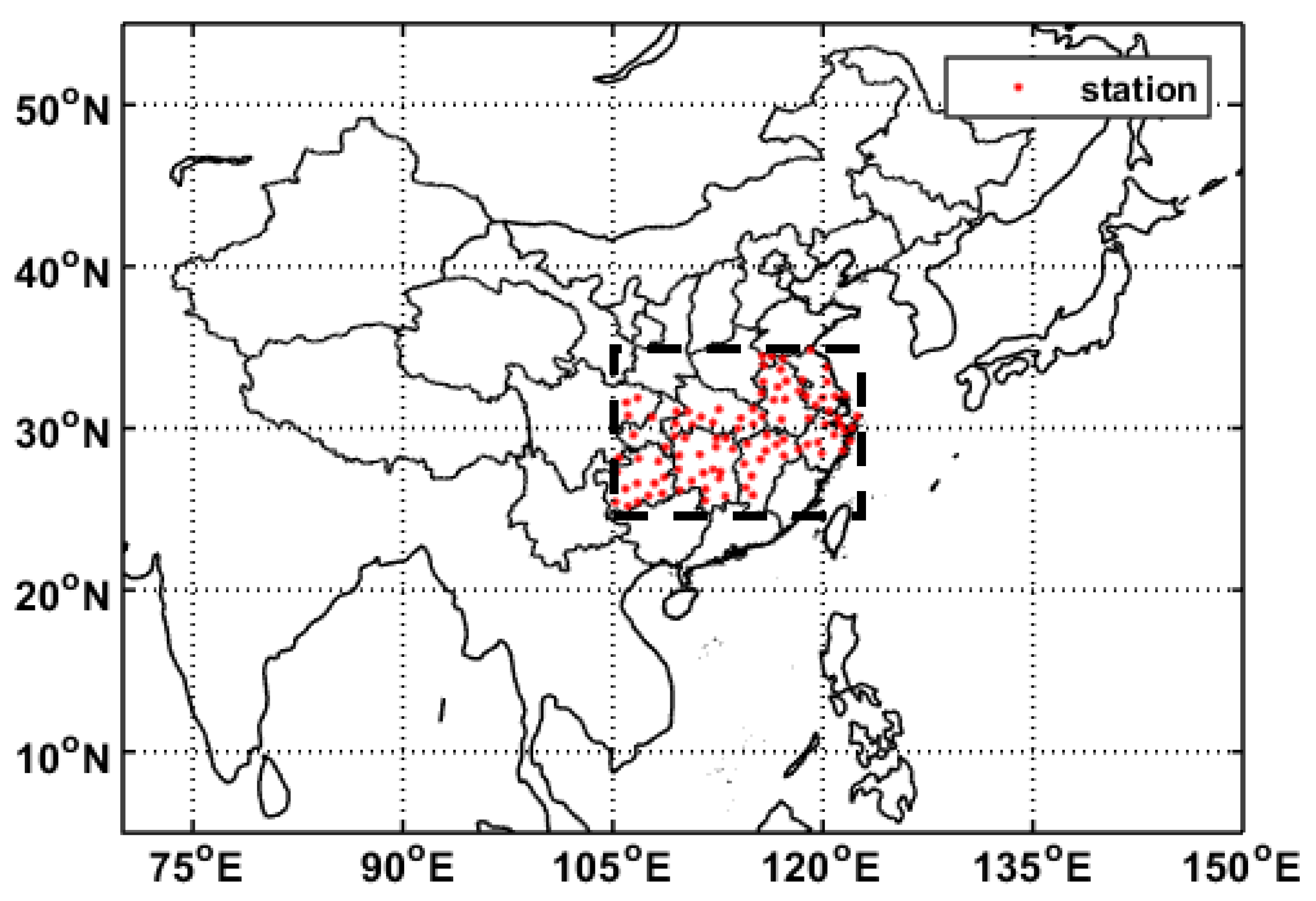
(1) In this article, precipitation data were selected from 97 meteorological stations with data covering the period 1980–2015. These gauge stations were almost evenly distributed within and surrounding the MLYRB (25°–35° N and 105°–122° E, Figure 1). The meteorological data were provided by the National Climatic Data Center, National Meteorological Information Center, and the China Meteorological Administration; the quality of the precipitation data was evaluated before its release. Missing data accounted for less than 1% of the total data and were processed following Zhang et al. [37]: rainfall values are calculated as the weighted average of all gauge stations and the weight of each station is determined by kriging interpolation. The fractal dimension can well represent the regional heterogeneity of the network under investigation [38]. According to the relevant literature, the fractal dimension of the study area in this paper is about 1.5 [39], which is in the range progressively from 0 (when all stations are distributed on a single point or on isolated points) to 2 (when all stations are uniformly distributed) [38]. Therefore, according to the judgment standards proposed by Lovejoy et al., the characteristics of precipitation distribution over the MLYRB can be characterized by the data of these stations. In this study, the four seasons were defined as spring (March–May), summer (June–August), autumn (September–November), and winter (December–February). To better characterize seasonal precipitation variations, we computed the seasonal precipitation anomalies by removing the 36-year average seasonal climatology, corresponding to the 1980–2015 period, from seasonal raw values. Subsequent analysis is based on AP anomalies over the MLYRB.

(2) A variety of monthly atmospheric circulation indices, such as the western Pacific subtropical high (WPSH) and QBO indices were sourced from the National Climate Center Climate System Diagnostic and Prediction Laboratory (NCC). Additionally, Niño 3.4 and Kuroshio Current SST (KCS) indices were calculated using the monthly Extended Reconstructed SST (ERSST) version 4 dataset [34] from the National Oceanic and Atmospheric Administration (NOAA) for the period 1980–2015 with a resolution of 2.5° * 2.5°. What needs to be emphasized here is that the indices and reanalysis data were analyzed at seasonal time-scale, and computed the seasonal anomalies for analysis.

(3) In the mechanism analysis section, monthly gridded data of 500 hPa geopotential height, 850 hPa wind horizontal components, and 700 hPa relative humidity were analyzed with a resolution of 2.5° * 2.5° from the National Centers for Environmental Prediction (NCEP) reanalysis dataset [40] for the period 1980–2015. We need to highlight that we computed the seasonal anomalies for reanalysis.

2.2. Methods

2.2.1. Empirical Orthogonal Function (EOF) Analysis

EOF analysis was used to identify the leading modes of seasonal precipitation variability affecting the MLYRB. The EOF approach has been extensively adopted for extracting the modes of variability explaining the largest portion of the total variance of the data [30,31,32,33]. Here, EOF analysis was conducted using AP anomalies over the MLYRB for the 1980–2015 period, resulting in a sample size of 36 cases.

2.2.2. Information Flow Causal Association Analysis Method

Pearson’s correlation coefficient is a metric commonly used to evaluate the linear relationships between two variables, providing the direction of deviations [32]. However, high and low correlations do not indicate the existence or absence of causal association between elements, which should be a primary consideration in forecasting, modelling, and physical mechanism assessments. Recently, Liang showed that causality can be regulated by using a closed form solution (defined as information flow, IF) derived from maximum likelihood estimation [41,42,43,44]. IF not only has indicated the exchange of causal information in linear systems, but also shown superior characteristics to the Granger causality test and transfer entropy in the causal analysis of nonlinear systems [45]. To accurately measure the relative size of a detected causal relationship, Liang developed an IF standardization method. For two time series, $x_2$ and $x_1$, the maximum likelihood estimator of the IF rate from $x_2$ to $x_1$ is [43]:

$$T_{2\to 1}=\frac{C_{11}{C}_{12}{C}_{2,d1}-C_{12}^2{C}_{1,d1}}{C_{11}^2{C}_{22}-C_{11}{C}_{12}^2}$$

(1)

Let ${\dot{X}}_j$ be the finite-difference approximation of $\frac{d{x}_j}{dt}$ using the Euler forward scheme:

$${\dot{X}}_{j,n}=\frac{X_{j,n+k}-X_{j,n}}{k\mathsf{\Delta }t}$$

(2)

where k = 1 or k = 2 and $\mathsf{\Delta }\mathrm{t}$ is the time step. The term $C_{i,j}$ in Equation (1) is the covariance between $x_i$ and $x_j$. Ideally, if $T_{2\to 1}=0$, then $x_2$ does not cause $x_1$; otherwise, it is causal. In practice, a significance test needs to be performed.

However, the results obtained in some cases would be very small (on the order of 0.001), which will not only make the contrast between the IF values of the variables inconspicuous, but also be inconsistent with our general intuitive understanding of standardized numerical ranges. Bai et al. proposed a standardization scheme with a new closed-form formula, which provided a reasonable solution to this limitation [46]. Moreover, Bai et al. verified the validity and robustness of this new standardized algorithm of information flow (NIF) through numerical simulation and forecasting experiments of tropical cyclone generation in the northwest Pacific Ocean. ${\tau }_{2\to 1}^B$ can be normalized as follows:

$${\tau }_{{}_{2\to 1}}^B=\frac{abs(T_{{}_{2\to 1}})}{abs(T_{{}_{2\to 1}})+abs(\frac{d{H}_1^{noise}}{dt})}$$

(3)

${\tau }_{2\to 1}^B$ measures the information flow from $x_2$ to $x_1$ in comparison to the stochastic processes. $H_1^{noise}$ represents the role of random noise. For additional information regarding his calculation process see Bai et al. [46]. The range of the values for ${\tau }_{2\to 1}^B$ is (0,1). The larger the value, the sharper the effect of $x_2$ on $x_1$ and the stronger the causal association (note the directionality); for relatively small values, the weighed element is not a fundamental factor for the development of $x_1$.

2.2.3. Bayesian Linear Regression Model

At present, climate predictions are usually produced and evaluated using physical and/or statistical models. The former are based on a set of differential partial equations and physical parameterizations representing different physical-dynamic processes in the atmosphere [47,48,49]. During recent years, such models have progressed in some aspects of precipitation predictions. However, owing to the nonlinearity of such physical models, errors generally increase rapidly for longer lead times, in particular for medium- and long-range forecasts [50]. To overcome the physical model’s limitation, statistical forecasting has been widely used for developing climate precipitation predictions, for instance [51,52]. One of the most employed methods in this crescent field is the use of the multiple linear regression (MLR) model [31,33,34]. The output of the MLR model can be interpreted as the most likely point estimate given by the current dataset. Nevertheless, if we have only a small dataset, the credibility of the point estimate based on the maximum probability given by the current dataset will be very low. In this case, if we represent the estimate as a distribution of possible values and introduce a regression model based on Bayesian theory, we may reduce the error to some extent [53]. Considering that the time span of the seasonal data of the precipitation is not large, for example, the sample length in this article is only 36, which is a small-sample problem. The Bayesian linear regression (BLR) model in this paper can introduce both prior information and uncertainty when having a limited dataset or needing to use a priori knowledge in the model [54].

3. The Leading Modes of Autumn Precipitation Variability over the MLYRB

Changes in precipitation can indicate variations in the hydrological cycle on regional or global scale [37]. To evaluate the main characteristics of the AP variability over the MLYRB from 1980 to 2015, we employed an EOF analysis on the seasonal rainfall anomalies using data from the 97 observational stations over the MLYRB. Here, we focused on the two leading modes, which show distinct interannual variability patterns. A rule of thumb (North et al. [55]) was used to assess the degree of degeneracy among EOF modes.

3.1. First Leading Mode

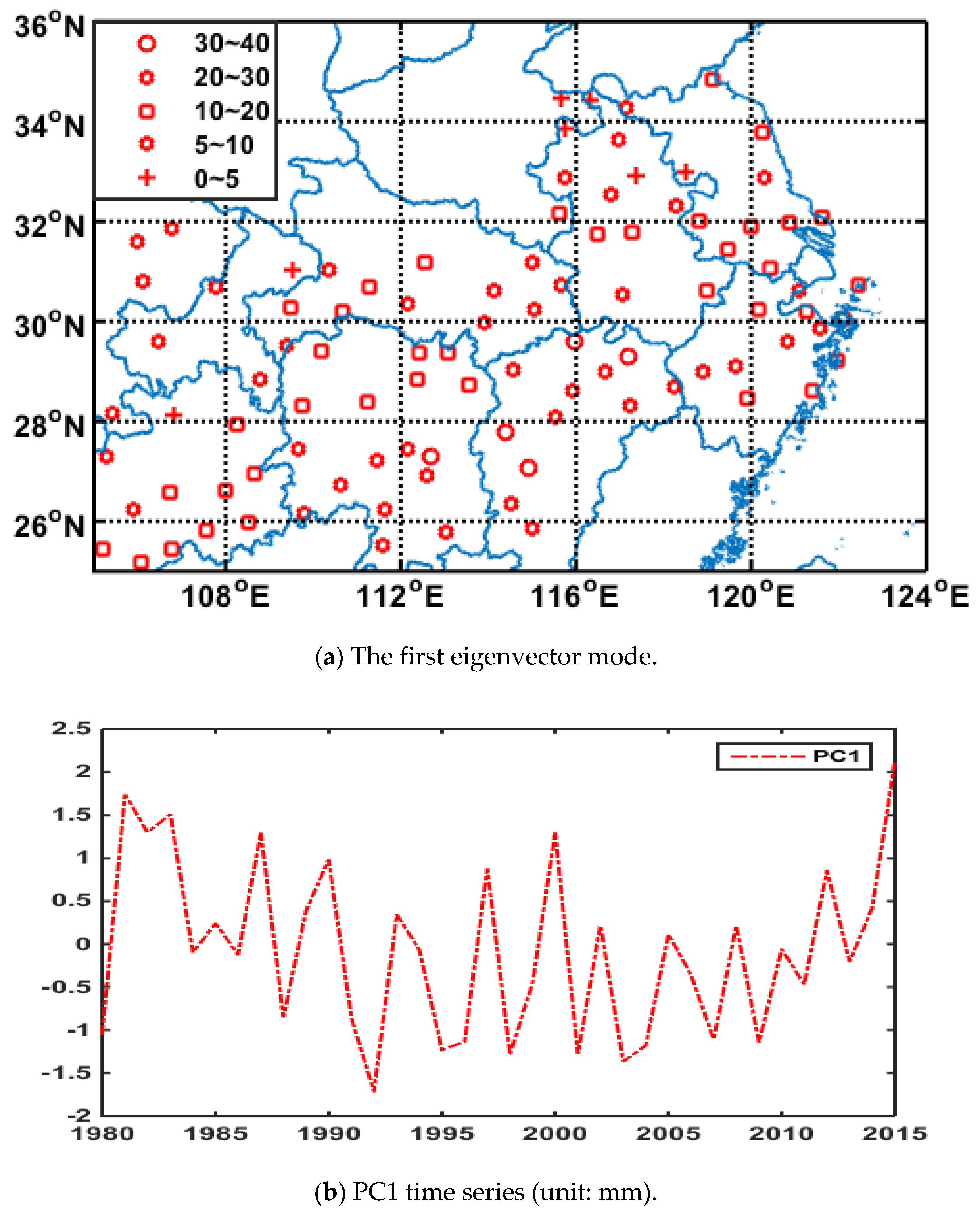
The first leading mode accounts for 30.83% of the total variance of AP anomalies. According to North et al. [55], this mode is independent of higher order modes. The first eigenvector (Figure 2a) shows a monopole with different precipitation amounts over the whole region. The temporal evolution of the first principal component (PC1) does not show a clear interdecadal variability during the 36-year period, while it shows significant interannual changes (Figure 2b).

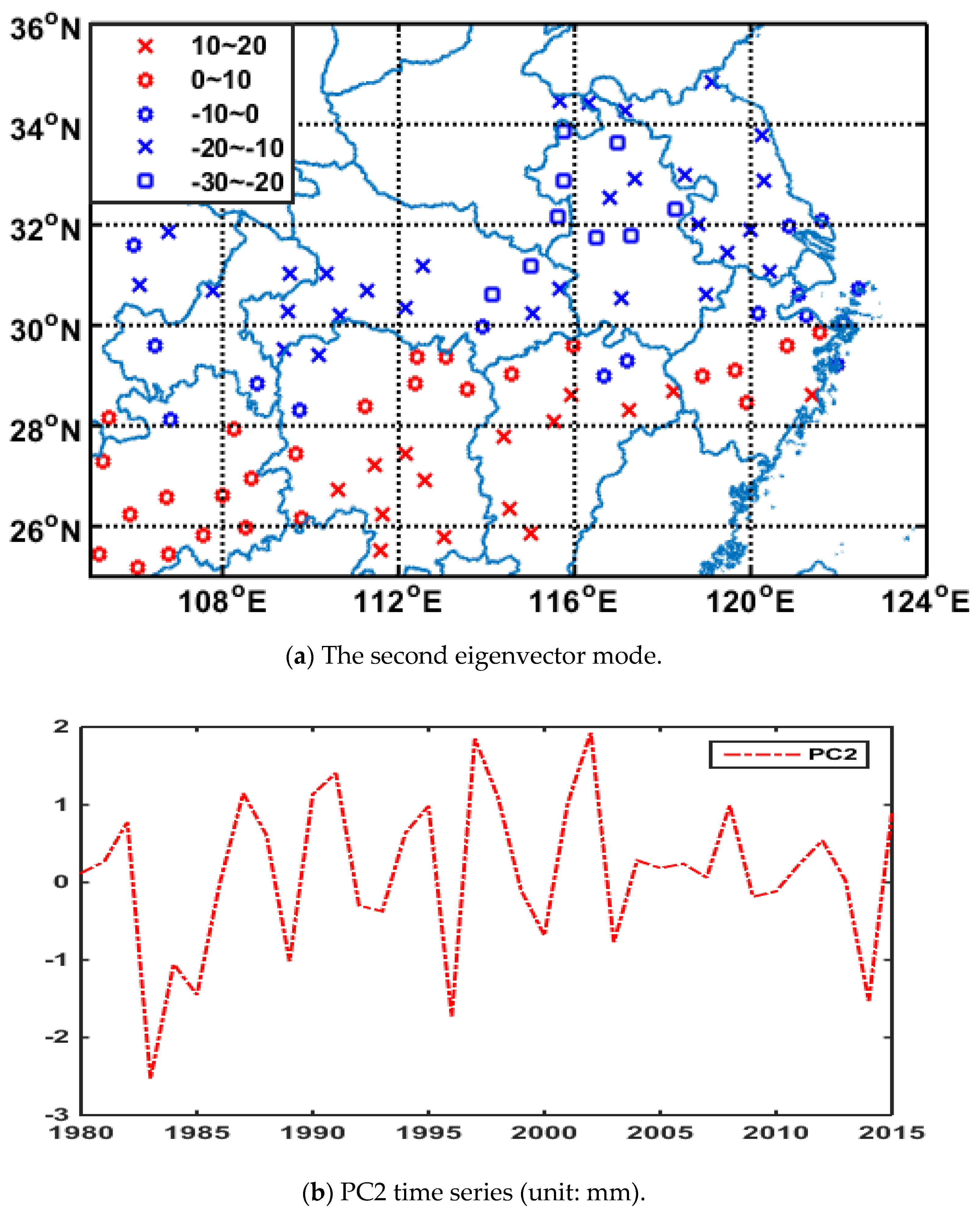
3.2. Second Leading Mode

The explained variance of the second mode is 16.13% and it is well separated from other EOF modes. AP anomalies exhibit a dipole-like pattern with a decreasing trend from southern to northern regions (Figure 3a). The temporal evolution of the second principal component (PC2) shows a clear interannual variability throughout the analyzed period (Figure 3b).

4. Extraction of the Main Modal Predictors of Autumn Precipitation Based on Information Flow Causality Detection

In this section, NIF is applied to the climate indices to extract the main climate predictors affecting the leading modes of AP variability over the MLYRB. Differently from a traditional statistical model, NIF focuses on identifying the most important predictors by understanding the causal relationships between potential predictors and predictands [46]. Both PCs (PC1 and PC2) are used to assess the most related climate indices that are causally associated with them. The correlation analysis (lead–lag correlation approach), which is commonly applied to evaluate climate predictions [33,34], is compared simultaneously to examine the effectiveness of the NIF method.

4.1. Potential Predictors for AP over the MLYRB

Based on previous studies, 13 climate indices (potential predictors) constitute the main scope for our investigation of predictors. They are classified as atmospheric circulation-, SST- and other slowly changing climate indices-based predictors.

4.1.1. Atmospheric Circulation Indices-Based Predictors

Many studies have shown that China precipitation anomalies are affected mainly by the western Pacific subtropical high (which controls warm and humid water vapor transport) and atmospheric circulation in the middle and high latitudes (which controls cold air transport from higher latitudes) [24,25,28,56,57]. In addition, atmospheric circulation conditions in the middle and high latitudes of the Northern Hemisphere can also be characterized by anomalies in the position and intensity of the 500 hPa ridges over the North Atlantic-Europe region (40°–80° N and 20° W–70° E). Five atmospheric circulation indices are selected to represent different tropical and extratropical circulation variability patterns.

Table 1. Definition of atmospheric circulation indices.

Climate Index	Definition
Atlantic-European Circulation W Pattern (AECW)	Number of days in the current month showing W-type circulation [28] (the 500 hPa circulation pattern of the North Atlantic-Europe is divided into W, C, and E patterns according to the differences in the ridge position and intensity in the North Atlantic-Europe region; the W type is characterized by a straight westerly circulation and prevailing zonal circulation.)
Atlantic-European Circulation C Pattern (AECC)	Number of days in the current month showing C-type circulation (the C type is characterized by high-pressure ridges over the western coast of Europe, long wave troughs in the Ural Mountains and the development of a meridional circulation in Europe) [28].
Atlantic-European Circulation E Pattern (AECE)	Number of days in the current month showing E-type circulation. The characteristics of the E type are opposite to those of the C type. The Ural Mountains exhibit a high-pressure ridge, and the pressure increases with longitude over East Asia [28].
Western Pacific Subtropical High Area (WPSHA)	In the 500 hPa geopotential height field, this index represents the spherical area of ≥ 5880 geopotential meters (gpm) in the 10°–60° N and 110°–180° E regions [28].
Arctic Oscillation (AO)	In the region of 20°–90° N and 0°–360°, this index signifies the normalized sequence of time coefficients of the first EOF mode of the 1000 hPa geopotential height anomaly field [28].

shows the definition of each index analyzed here. It should be noted that the seasonal indices were analyzed only for summer season and obtained by computing 3-month mean using the corresponding monthly data.

4.1.2. SST Indices-Based Predictors

Many studies have shown that the precipitation anomalies in China are often related to SST anomalies, especially in the tropical Pacific and Indian Oceans [25,27,28,56,57]. These studies have verified that El Niño, La Niña, the large cold water mass close to Japan (associated with the Kuroshio Current SST), Indian Ocean Dipole, and other climate phenomena affect China’s precipitation through complex mechanisms. Among the six SST indices assessed here, two new indices were defined to clarify both the relationships between different SST anomalies distributions in the tropical Pacific Ocean and different China precipitation anomalous patterns. The first new SST index is the East-West index (EWI), which is the difference between the normalized Niño 3 index (defined as the regional average of monthly SST anomalies in the 5° S–5° N and 150°–90° W region, representing the tropical eastern Pacific) and the tropical western Pacific index (defined as the regional average of monthly SST anomalies in the 5° S–5° N and 110°–160° E region), reflecting the SST variability between the east and west tropical Pacific. The second new SST index is the East-Central index (ECI), which is the sum of the standardized Niño 3 index and the Niño 4 index (defined as the regional average of monthly SST anomalies in the 5° S–5° N and 160° E–150° W region, representing the tropical central Pacific), reflecting the consistent SST variability in the tropical central and eastern Pacific Ocean.

Table 2. Definition of SST indices.

Climate Index	Definition
NINO3.4 SSTA (NINO3.4)	Regional average of the SST anomaly in the region of 5° S–5° N and 170°–120° W [22]
Kuroshio Current SSTA (KCS)	Regional average of the SST anomaly in the regions of 35° N and 140°–150° E and 25°–30° N and 125°–150° E [27].
Tropical Indian Ocean Dipole (TIOD)	Difference between the regional averages of the SST anomalies in the 10° S–10° N and 50°–70° E and 10° S–0° and 90°–110° E regions [25].
Sub-Indian Tropical Dipole (SIOD)	Difference between the regional averages of the SST anomalies in the 45°–30° S and 45°–75° E and 25° S–15° S and 80°–100° E regions [25].
East-West index (EWI)	Anomalous distribution characteristics of the Tropical Pacific SST in the east and west.
East-Central index (ECI)	Consistent variation in the SST anomalies in the tropical central and eastern Pacific.

shows the definition of each SST index calculated from the ERSST dataset for summer season over the 1980–2015 period.

4.1.3. Potential Predictors of Low-Frequency Climate Signals

Some studies have shown that AP in China can be affected by other slowly changing climate indices, such as the QBO [29]. Other studies have also noted that abnormal solar activity may also affect precipitation in local areas [58,59]. Therefore, we included the QBO index (defined as the 30 hPa zonal wind average in the equatorial region) and total sunspot number index (TSN; relative number of sunspots) as the potential predictors to be also investigated. To eliminate subjective factors and irregular disturbances in the observations, a 12-month moving average of the relative number of sunspots is used; this dataset is also from the NCC.

4.2. Assessing the Predictors Affecting the First EOF Mode

In this section, we use the NIF to detect the causal relationship between each climate index and PC1. The reliability test follows the methodology proposed by Liang: if the standardized IF value is ≥ 0.01, the result is statistically significant with a 95% confidence level [43]. All results are listed in

Table 3. Information flow (IF) ${\tau }_{Col\to Row}^B$ values between PC1 and the atmospheric circulation indices-based predictors (bold font indicates statistically significant values at the 5% level, and 0.00 means the value is less than 0.005; the same applies to the following tables).

${\mathit{\tau }}_{{}_{\mathit{C}\mathit{o}\mathit{l}\to \mathit{R}\mathit{o}\mathit{w}}}^{\mathit{B}}$	WPSHA	AECW	AECC	AECE	AO
PC1	0.03	0.01	0.00	0.01	0.01

,

Table 4. IF ${\tau }_{Col\to Row}^B$ values between PC1 and the SST indices-based predictors (bold font indicates statistically significant values at the 5% level).

${\mathit{\tau }}_{{}_{\mathit{C}\mathit{o}\mathit{l}\to \mathit{R}\mathit{o}\mathit{w}}}^{\mathit{B}}$	NINO3.4	KCS	TIOD	SIOD	EWI	ECI
PC1	0.13	0.13	0.16	0.12	0.15	0.13

and

Table 5. IF ${\tau }_{Col\to Row}^B$ values between PC1 and the low-frequency climate indices (bold font indicates statistically significant values at the 5% level).

${\mathit{\tau }}_{{}_{\mathit{C}\mathit{o}\mathit{l}\to \mathit{R}\mathit{o}\mathit{w}}}^{\mathit{B}}$	QBO	TSN
PC1	0.04	0.05

, and it is necessary to indicate that the IF direction is transmitted from the column indicator to the line indicator.

From Table 3, Table 4 and Table 5, most climate indices are statistically significant and show causal associations with PC1 (except AECC). Among indices, TIOD has the largest IF, showing the Indian Ocean SST anomaly modulation on AP over the MLYRB. Previous studies have already reported such relationships between these climate indices. For example, Zhang et al. proposed that the TIOD directly promotes the development of the Indian-Burma trough, which, in turn, modulates the water vapor transport from the Indian Ocean and South China Sea to eastern China [57]. The two new SST indices (EWI and ECI) have also a relatively large impact on PC1. By comparing the IF values of these indices, we can further verify that the difference between SST anomalies in the west and east tropical Pacific Ocean (EWI) have a more significant impact on the first EOF mode.

The same data are also evaluated using linear correlation analysis (

Table 6. Correlation coefficients (R) between PC1 and the Atmospheric circulation indices-based predictors (bold font indicates statistically significant values at the 5% level).

R	WPSHA	AECW	AECC	AECE	AO
PC1	−0.07	0.15	0.00	−0.17	−0.19

,

Table 7. Correlation coefficients (R) between PC1 and the SST indices-based predictors (bold font indicates statistically significant values at the 5% level).

R	NINO3.4	KCS	TIOD	SIOD	EWI	ECI
PC1	0.36	−0.15	0.37	0.11	0.48	0.36

and

Table 8. Correlation coefficients (R) between PC1 and the low-frequency climate indices (bold font indicates statistically significant values at the 5% level).

R	QBO	TSN
PC1	0.26	0.14

; correlation coefficient uses the F test [25,46]. Since the sample size of this article is 36, R $\ge 0.325$ indicates statistically significant values at the 5% level.). With the exceptions of EWI, ECI, TIOD, and NINO3.4, most climate indices do not show statistically significant relationships, differing from previous studies. For example, Liu and Yu suggested that changes in AO have important influence on intensity and cold air flow path in autumn, and this cold air has a considerable impact on China AP [25]. Gu et al. verified that SIOD plays an important role in promoting the formation of TIOD [56]. However, correlation analysis cannot significantly reflect associations between these climate indices and PC1. In contrast, both indices are meaningful in the NIF assessment, which is in good agreement with previous studies. NIF can reflect time-lagged relationships between the equatorial Pacific SST anomalies and precipitation variability. For example, the IF from EWI to PC1 is 0.12 at the same season, which is smaller than the NIF value for one season later, as shown in Table 4. Moreover, this finding was not observed using correlation analysis (i.e., simultaneous correlation: 0.51; time-lagged correlation: 0.48).

4.3. Assessing the Predictors Affecting the Second EOF Mode

The results at

Table 9. IF ${\tau }_{Col\to Row}^B$ values between PC2 and the Atmospheric circulation-indices based predictors (bold font indicates statistically significant values at the 5% level).

${\mathit{\tau }}_{{}_{\mathit{C}\mathit{o}\mathit{l}\to \mathit{R}\mathit{o}\mathit{w}}}^{\mathit{B}}$	WPSHA	AECW	AECC	AECE	AO
PC2	0.00	0.08	0.17	0.27	0.06

,

Table 10. IF ${\tau }_{Col\to Row}^B$ values between PC2 and the SST-indices based predictors (bold font indicates statistically significant values at the 5% level).

${\mathit{\tau }}_{{}_{\mathit{C}\mathit{o}\mathit{l}\to \mathit{R}\mathit{o}\mathit{w}}}^{\mathit{B}}$	NINO3.4	KCS	TIOD	SIOD	EWI	ECI
PC2	0.12	0.13	0.02	0.06	0.03	0.09

,

Table 11. IF ${\tau }_{Col\to Row}^B$ values between PC2 and the low-frequency climate indices (bold font indicates statistically significant values at the 5% level).

${\mathit{\tau }}_{{}_{\mathit{C}\mathit{o}\mathit{l}\to \mathit{R}\mathit{o}\mathit{w}}}^{\mathit{B}}$	QBO	TSN
PC2	0.08	0.00

,

Table 12. Correlation coefficients (R) between PC2 and the Atmospheric circulation-indices based predictors (bold font indicates statistically significant values at the 5% level, and −0.00 means the value is less than −0.005).

R	WPSHA	AECW	AECC	AECE	AO
PC2	−0.00	−0.17	0.23	−0.36	−0.26

,

Table 13. Correlation coefficients (R) between PC2 and the SST-indices based predictors (bold font indicates statistically significant values at the 5% level).

R	NINO3.4	KCS	TIOD	SIOD	EWI	ECI
PC2	0.35	0.45	−0.04	−0.23	0.20	0.29

and

Table 14. Correlation coefficients (R) between PC2 and the low-frequency climate indices (bold font indicates statistically significant values at the 5% level).

R	QBO	TSN
PC2	0.1832	0.0142

show that NINO3.4, KCS, AECE, ECI, and QBO are the main climate indices affecting the second mode of AP variability over the MLYRB. Compared to the correlation coefficient assessment, the NIF can more accurately indicate which climate indices most affect PC2. For example, when AECE is abnormal, the Ural Mountains exhibit a high-pressure ridge, and the pressure increases with longitude over East Asia, which usually indicates a cold air anomaly [28]; this may be an important reason for the second mode to show an antiphase north-south variation trend. Shi verified that SST variations in the Kuroshio Current can modulate AP over the Yangtze River Basin [27], which could explain the AP anomalies over northern regions from 29° N.

5. Effectiveness of Predictors’ Detection Based on Regression Analysis

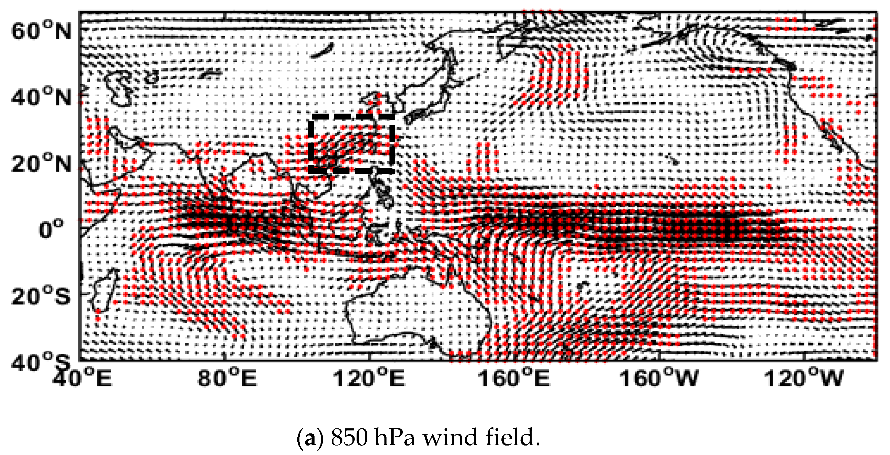
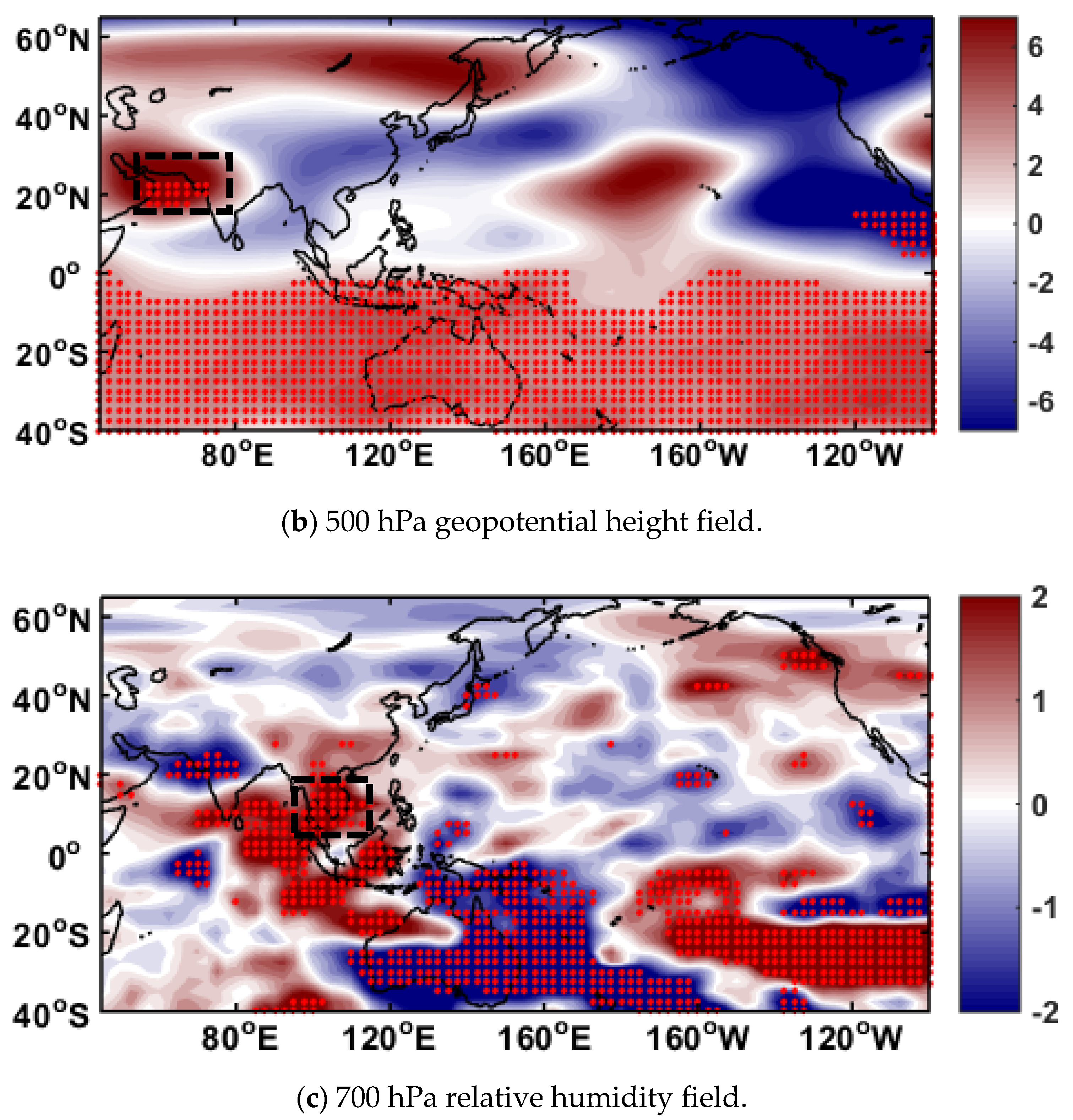
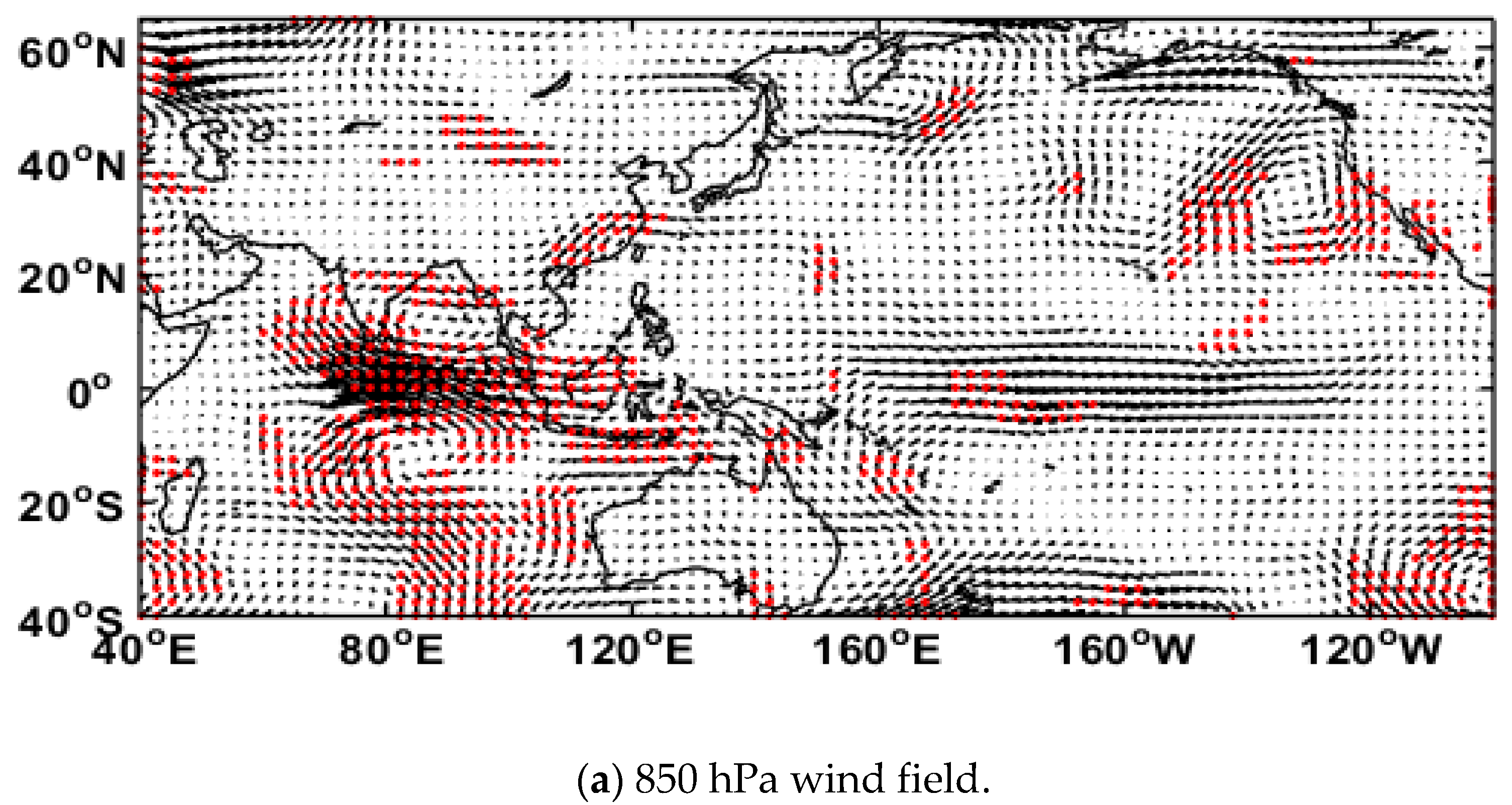
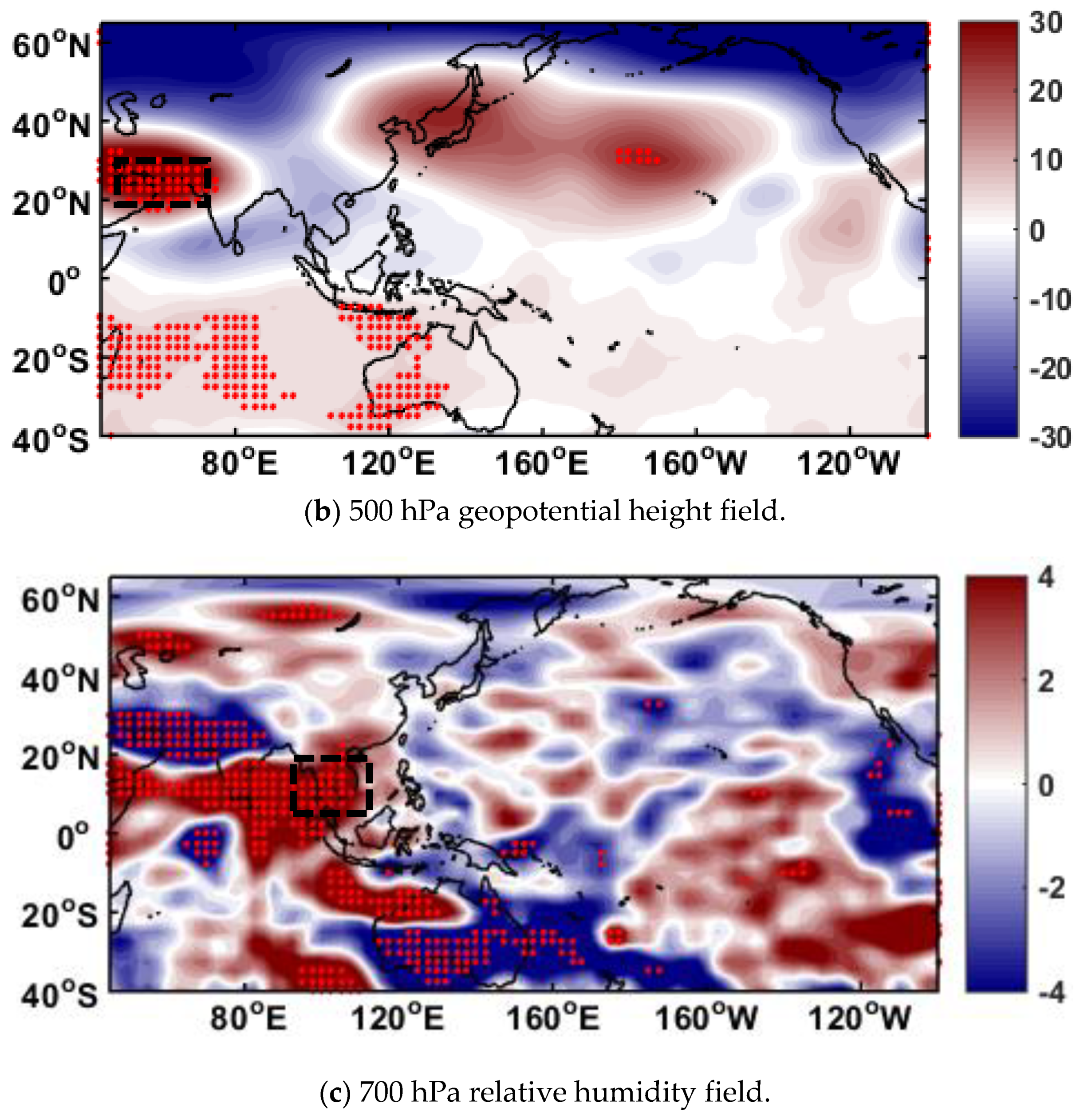
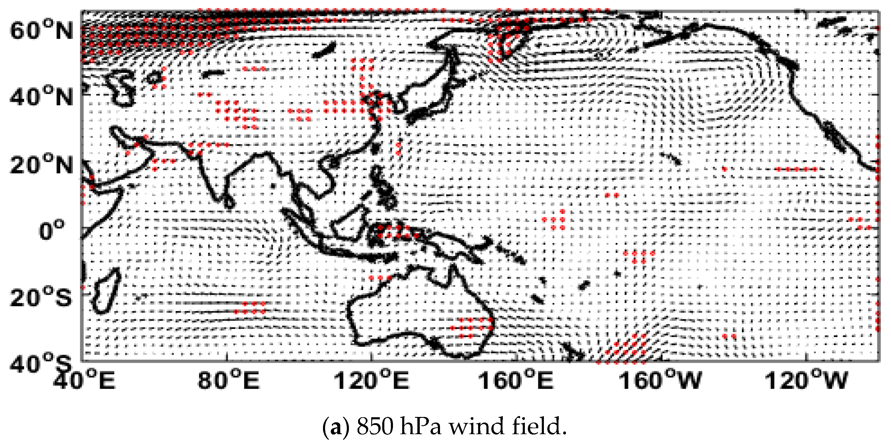
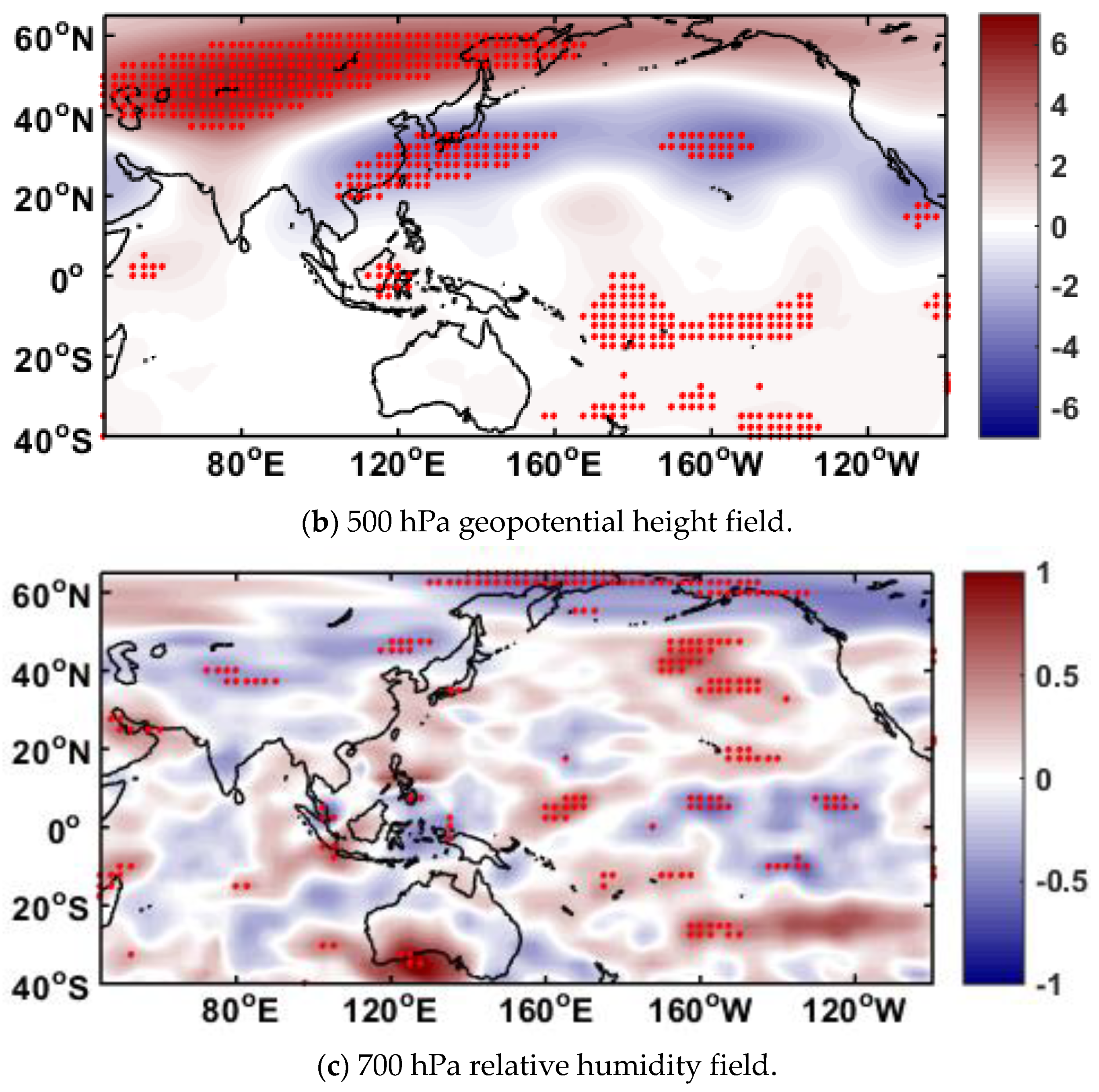
To further verify the usefulness of the NIF, this section evaluates the two most significant climate indices related to PC1 variability (EWI, TIOD) by computing the linear regression between these indices and different dynamic and thermodynamic variables affecting China AP [57]. For comparison, similar regression analysis is also employed using the AECC index that showed weakest association with PC1. Regression coefficients are calculated using time-lagged anomalies with summer indices defined as predictors and AP as the predicted variable. In this article, we use the F test to test the significance of the regression coefficients. The F test is a test of the goodness of fit of the entire model, that is, the significance test of all variables to the explanatory variables [25]. Figure 4, Figure 5 and Figure 6 show the variations in the regressed fields of the 700 hPa relative humidity, 850 hPa atmospheric circulation, and 500 hPa geopotential height with respect to the different climate indices. All of these regressed fields also support the conclusions provided by the NIF. As shown in Figure 4, due to the anomalous east-west distribution of the tropical Pacific SST, a strong westward airflow was stimulated over the tropical Pacific, and an easterly airflow occurred in the Indian Ocean at 850 hPa. After the eastward airflow crossed the Indo-China Peninsula, the airflow turned into a southwestern airstream and entered southwestern China (the dashed squares in Figure 4a and Figure 5a). Furthermore, a large-scale anomalous southwesterly airflow over East China is observed. The 700 hPa relative humidity anomalies over the Indo-China Peninsula and Philippines (the dashed squares in Figure 4c and Figure 5c) are verified to be most likely related to the 850 hPa atmospheric circulation anomalies. These mechanisms are relevant to produce AP anomalies over the MLYRB, especially in the southern region, which is in good agreement with the spatial distribution of the first EOF mode. In Figure 5, an easterly airflow was stimulated mainly over the tropical Indian Ocean owing to the TIOD. This easterly airflow was deflected to the north over the Indian Peninsula and then developed eastward, modulating a southwestern anomalous airflow over East China. Geopotential height anomalies were also enhanced in the India-Burma trough (the dashed squares in Figure 4b and Figure 5b), but it must be highlighted that this field passed only the 90% confidence interval test and not the 95% confidence interval test. In Figure 6, the relative humidity and circulation fields showed weak regression coefficients, indicating that AECC has a negligible effect in modulating the first EOF mode. This finding is consistent with results presented in Table 3. Therefore, the proposed NIF assessment can accurately reveal the most important climate drivers affecting the leading mode of AP variability over the MLYRB.

6. Prediction Experiment of AP over MLYRB

To achieve an acceptable prediction performance, we first obtain two ranked lists of climate indices ordered according to the values of the NIF and correlation coefficients based on Table 3, Table 4, Table 5, Table 6, Table 7, Table 8, Table 9, Table 10, Table 11, Table 12, Table 13 and Table 14. Then, as recommended by Song et al. [60], we selected the top k factors from these two ranking lists, where $k=\sqrt{m}\ast \ln m$ and $m$ is the number of potentially selected indices. In this study, the number of climate indices is 13, and k = 8. Thus, the top eight common indices in the two ranked lists are chosen as the final predictors. Following this procedure, KCS, TIOD, SIOD, EWI, WPSHA, and AO are the six most important predictors affecting PC1; NINO3.4, KCS, AECE, AECC, ECI, and QBO are the major predictors for PC2. Therefore, in this section, we analyze BLR prediction quality in coordination with these selected climatic factors and compare the BLR with the output of MLR, which is a common assessment in climate prediction. To reduce the impacts of the data from the current year on the forecasting results, when applying the MLR model, the regression forecast is performed with a cross-validation assessment excluding the target year. The BLR model can be simply expressed by Equation (4):

$$\mathrm{PC}=\mathrm{g}+\left\{\mathrm{a},\mathrm{b},\mathrm{c},\mathrm{d},\mathrm{e},\mathrm{f}\right\}\ast \mathrm{SX}$$

(4)

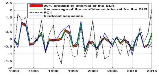
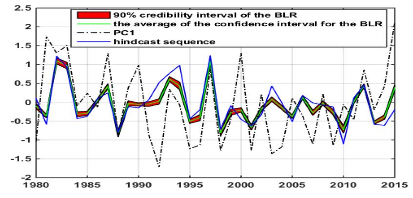
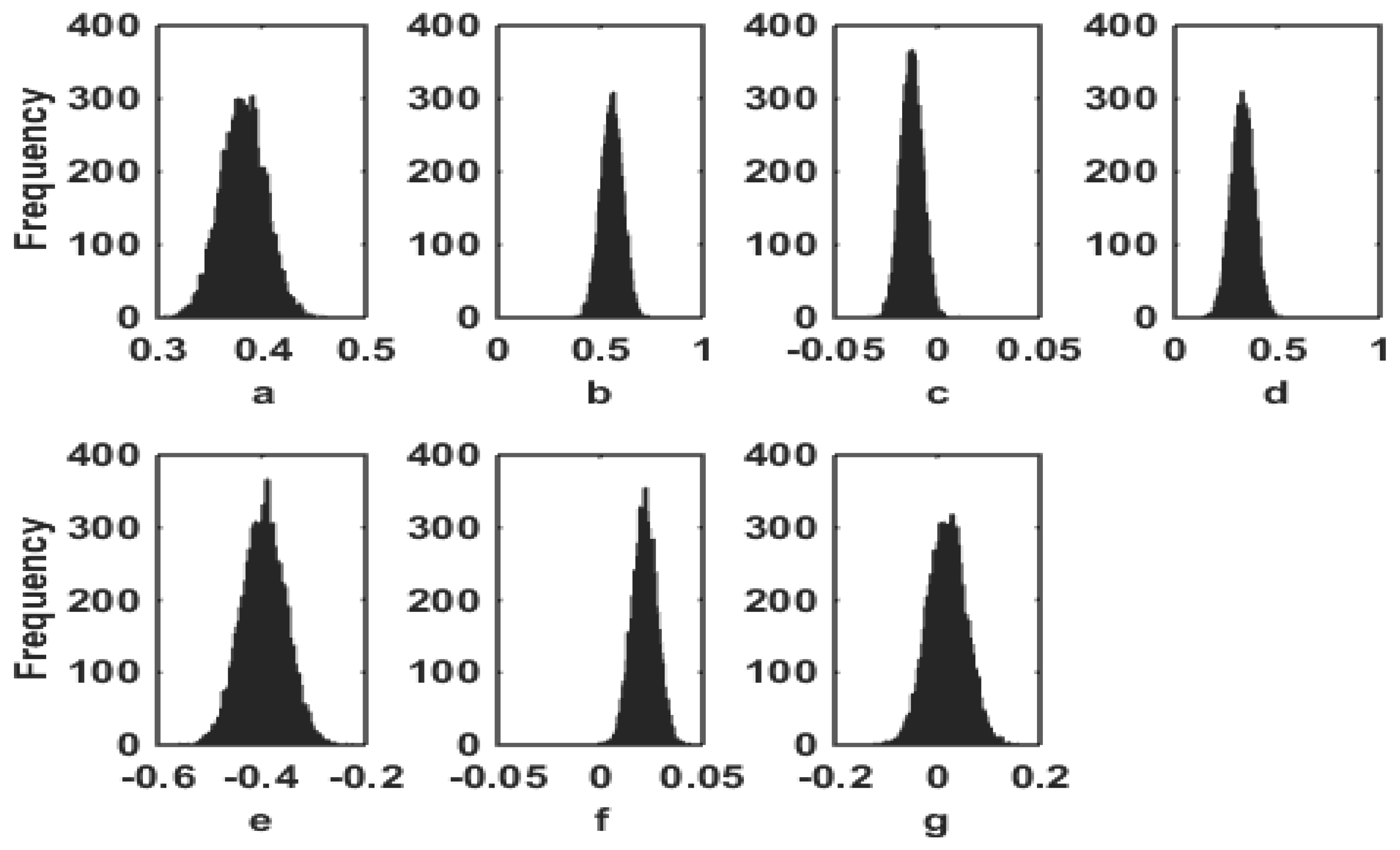
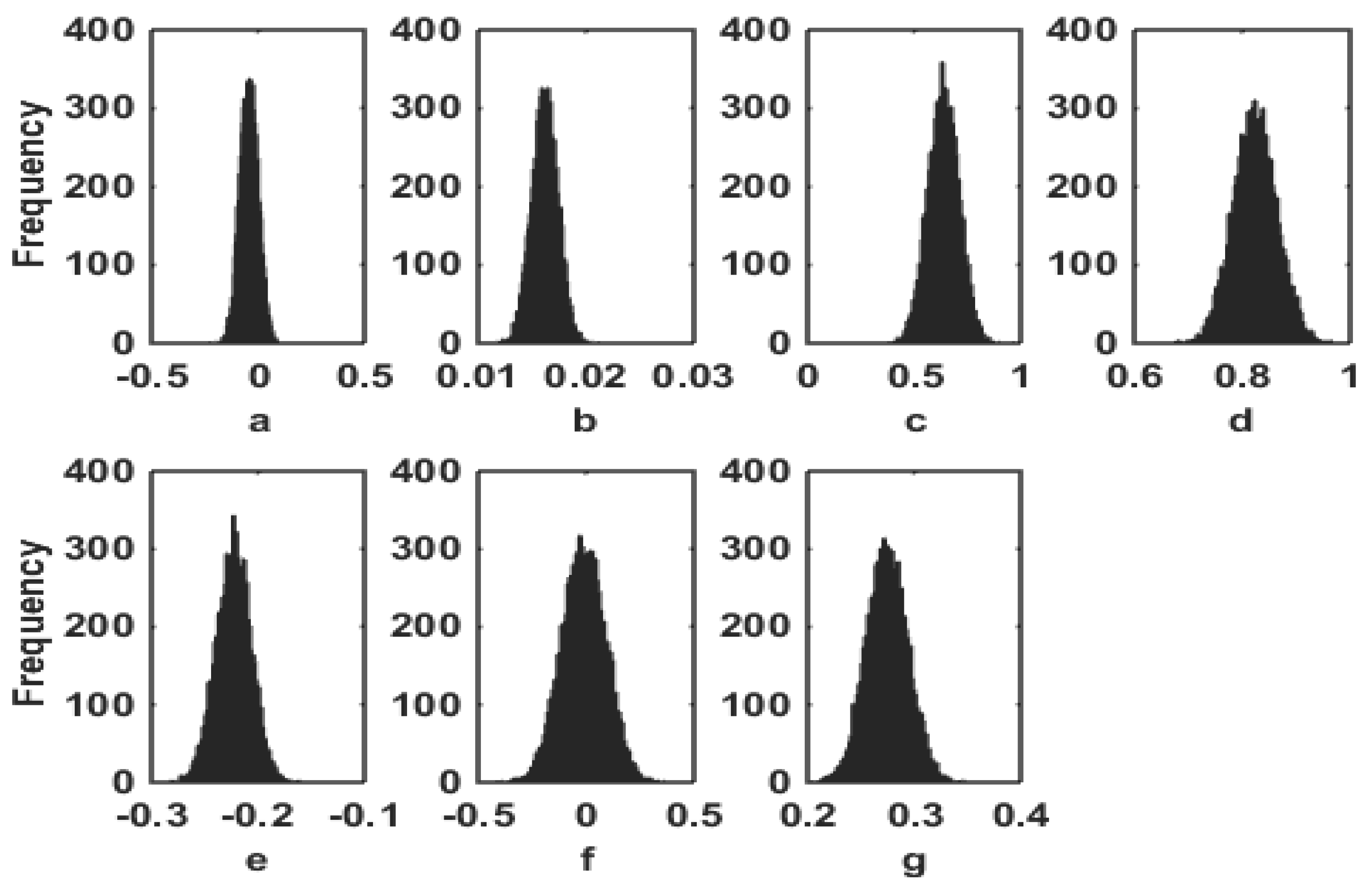
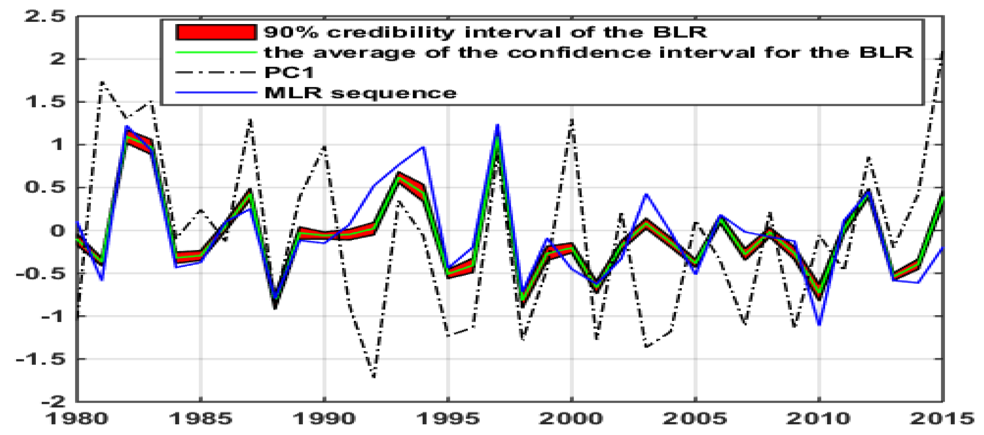
where g is a constant term and SX is a set of predictors with a, b, c, d, e, and f being their corresponding parameters. The histograms of the regression parameters $\left\{\mathrm{a},\mathrm{b},\mathrm{c},\mathrm{d},\mathrm{e},\mathrm{f}\right\}$ are shown in Figure 7 and Figure 8. The final regression results are shown in Figure 9 and Figure 10, where the red area represents the 90% confidence interval predicted by BLR and the green solid line represents the interval average predicted by BLR. The multiple correlation coefficient (MCC) and root mean square error (RMSE) are introduced to measure the specific performance of the forecast results [46]. Regression assessment is calculated using time-lagged anomalies, which considers using summer indices to predict AP anomalies.

According to the regression results for the time series of PC1 (Figure 9), the BLR model captured the decreasing trend in 2006–2007, the increasing pattern in 2007–2008 and 2011-2012, the decreasing trend in 2012, and the increasing pattern in 2013. From the comparison results in

Table 15. Skill scores (in terms of the multiple correlation coefficient (MCC) and root mean square error (RMSE)) for the PC1 forecast by different models (bold font indicates the best performance).

Judging Index	MLR	BLR
MCC	0.2019	0.5299
RMSE	1.0418	0.8508

, the prediction results for the first mode of the BLR model are more satisfactory than those of the MLR model; the MCC of the BLR model is 0.5299, and the RMSE is 0.8508, which are significantly better than those of the MLR model. The BLR model forecast quality, when evaluated by the MCC and RMSE scores, showed an improvement of around 40% compared to the MLR model. The related forecasting results also reflect how useful the NIF assessment is for extracting potential forecasting factors from the margins of the studied domain. Compared to the traditional scheme (MLR) [33,34], the BLR scheme better predicts the trend of interannual changes in AP over the MLYRB.

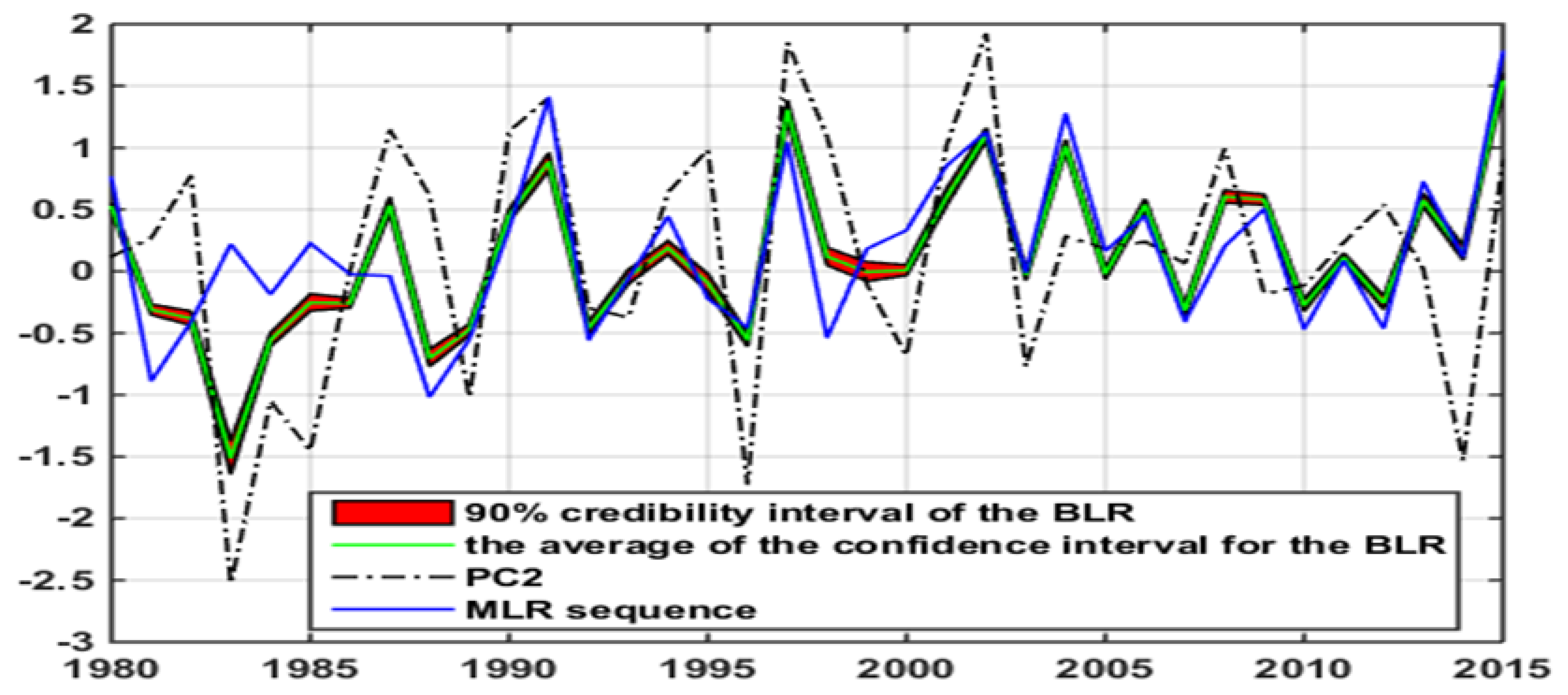
The prediction results for the PC2 time series (Figure 10) reveal that the BLR captured the upward trend in 1989–1991, the downward pattern in 1991–1992 and 2002–2003, the decreasing trend in 2013, and the increasing pattern in 2015. As seen from

Table 16. Skill scores for the PC2 forecast by different models (bold font indicates the best performance).

Judging Index	MLR	BLR
MCC	0.3216	0.6727
RMSE	0.9921	0.7358

, the performance of the BLR is also satisfactory, with an MCC of 0.6727 and an RMSE of 0.7358. A comparison between BLR and MLR models shows that the former forecast quality, when evaluated by the MCC and RMSE scores, showed an improvement around 35% and 26% compared to the latter, respectively.

7. Discussion

Although the prediction skills of AP over the MLYRB using the NIF-BLR model are superior, there are still some limitations. First, most of the climate indices proposed in this study were selected from previous research, which led to certain subjectivity in the evaluation process. As a future step, we will further develop research combining numerical forecasting model products to improve the quality of forecasts. Second, if the cycle of the regression model changes, this may lead to a decrease in the prediction skill. Thus, the prediction model established in this study may not be fully applicable to other periods. Therefore, in the later period, we will carry out further research in combination with numerical forecasting models to improve the quality of forecasts. One way to undertake this evaluation is using the projection of the model’s hindcast anomalies (we will select an appropriated climate model for providing hindcast data) onto the two observed leading eigenvectors (we already have this) to obtain the corresponding forecasted PC time series. Despite these potential limitations, the prediction factors and precipitation prediction results identified in this study will help us to better understand the variability in autumn precipitation over the MLYRB and improve the regional prediction of autumn precipitation elsewhere. These findings may also help policymakers and decision makers to prepare appropriate adaptation and mitigation measurements for future climate change.

8. Summary

This study investigated the characteristics of AP anomalies over the MLYRB by exploring the leading spatial-temporal modes and potential predictors driving the precipitation variability. The main conclusions are as follows:

(1) Regarding EOF analysis, the MLYRB is a region with significantly varying AP. The contribution of the variance in the first leading mode is 30.83% and shows a monopole with different precipitation amounts over the whole region. The second mode explains 16.13% of the total variance, and its spatial distribution function is characterized by a meridional dipole. The time series of the first two PCs shows marked interannual variations, but weak interdecadal signals.

(2) To achieve an acceptable prediction performance, we firstly obtained two ranked lists of climate indices ordered according to the values of the NIF and correlation coefficients. Then, as recommended by Song et al. [60], we selected the top eight factors from the two ranked lists. Thus, the top eight common indices in the two ranked lists were chosen as the final predictors. Following this procedure, KCS, TIOD, SIOD, EWI, WPSHA, and AO are the six most important predictors affecting the first EOF mode of AP over the MLYRB, whereas NINO3.4, KCS, AECE, AECC, ECI, and QBO are the major predictors for the second mode.

(3) We considered the time series prediction of the first two PCs as a small-sample problem; therefore, the BLR model could be adopted. From the experimental results, BLR captured the PC1 and PC2 trends, and the overall performance was relatively satisfactory. Finally, the BLR demonstrates the ability to improve upon the MLR model.

References

- Kurane, I. The effect of global warming on infectious diseases. Osong Public Health Res. Perspect. 2010, 1, 4–9. [Google Scholar] [CrossRef] [Green Version]
- Yu, M.; Li, Q.; Hayes, M.J.; Svobodab, M.D.; Heim, R.R. Are droughts becoming more frequent or severe in China based on the Standardized Precipitation Evapotranspiration Index: 1951–2010? Int. J. Climatol. 2014, 34, 545–558. [Google Scholar] [CrossRef]
- Tian, Q.; Prange, M.; Merkel, U. Precipitation and temperature changes in the major Chinese river basins during1957–2013 and links to sea surface temperature. J. Hydrol. 2016, 536, 208–221. [Google Scholar] [CrossRef]
- Cui, L.; Wang, L.; Lai, Z.; Tian, Q.; Liu, W.; Li, J. Innovative trend analysis of annual and seasonal air temperature and rainfall in the Yangtze River Basin, China during 1960–2015. J. Atmos. Sol. Terr. Phys. 2017, 164, 48–59. [Google Scholar] [CrossRef]
- O’Gorman, P.A.; Schneider, T. The physical basis for increases in precipitation extremes in simulations of 21st-century climate change. Proc. Natl. Acad. Sci. USA 2009, 106, 14773–14777. [Google Scholar] [CrossRef] [Green Version]
- Xu, Y.; Xu, C.; Gao, X.; Luo, Y. Projected changes in temperature and precipitation extremes over the Yangtze River basin of China in the 21st century. Quat. Int. 2009, 208, 44–52. [Google Scholar] [CrossRef]
- Schiermeier, Q. Climate and weather: Extreme measures. Nature 2011, 477, 148–149. [Google Scholar] [CrossRef]
- Liu, J.; Wang, B.; Cane, M.A.; Yim, S.Y.; Lee, J.Y. Divergent global precipitation changes induced by natural versus anthropogenic forcing. Nature 2013, 493, 656–659. [Google Scholar] [CrossRef]
- Gocic, M.; Trajkovic, S. Analysis of changes in meteorological variables using Mann-Kendall and Sen’s slope estimator statistical tests in Serbia. Glob. Planet. Chang. 2013, 100, 172–182. [Google Scholar] [CrossRef]
- IPCC. Climate Change 2013: The Physical Science Basis. Contribution of Working Group I to the Fifth Assessment Report of the Intergovernmental Panel on Climate Change; Cambridge University Press: Cambridge, UK, 2013; pp. 1–1535. [Google Scholar]
- Wang, L.; Chen, Y.; Niu, Y.; Salazar, G.; Gon, W. Analysis of atmospheric turbidity in clear skies at Wuhan, Central China. J. Earth Sci. 2017, 28, 729–738. [Google Scholar] [CrossRef]
- Allen, S.K.; Plattner, G.K.; Nauels, A.; Xia, Y.; Stocker, T.F. Climate change 2013: The physical science basis. an overview of the working group 1 contribution to the fifth assessment report of the intergovernmental panel on climate change (IPCC). Comput. Geometry. 2007, 18, 95–123. [Google Scholar]
- Alexander, L.V.; Zhang, X.; Peterson, T.C.; Caesar, J.; Gleason, B.; Klein Tank, A.M.G.; Haylock, M.; Collins, D.; Trewin, B.; Rahimzadeh, F.; et al. Global observed changes in daily climate extremes of temperature and precipitation. J. Geophys. Res. Atmos. 2006, 111, 1042–1063. [Google Scholar] [CrossRef] [Green Version]
- Donat, M.G.; Alexander, L.V.; Yang, H.; Durre, I.; Vose, R.; Caesar, J. Global land-based datasets for monitoring climatic extremes. Bull. Am. Meteorol. Soc. 2013, 94, 997–1006. [Google Scholar] [CrossRef] [Green Version]
- Mallakpour, I.; Villarini, G. The changing nature of flooding across the Central United States. Nat. Clim. Chang. 2015, 5, 250–254. [Google Scholar] [CrossRef]
- Villarini, G.; Smith, J.A.; Vecchi, G.A. Changing frequency of heavy rainfall over the Central United States. J. Clim. 2013, 26, 351–357. [Google Scholar] [CrossRef]
- Su, B.; Jiang, T.; Ren, G.Y.; Chen, Z.H. Observed trends of precipitation extremes in the Yangtze River basin during 1960 to 2004. Adv. Clim. Chang. Res. 2006, 2, 9–14. [Google Scholar]
- Fu, G.; Yu, J.; Yu, X.; Ouyang, R.; Zhang, Y.; Wang, P.; Liu, W.; Min, L. Temporal variation of extreme rainfall events in China, 1961–2009. J. Hydrol. 2013, 487, 48–59. [Google Scholar] [CrossRef]
- Ren, G.Y.; Ren, Y.Y.; Zhan, Y.J.; Sun, X.B.; Ren, G.Y.; Ren, Y.Y.; Zhan, Y.J.; Sun, X.B.; Zhang, L.; Ren, Y.Y.; et al. Spatial and temporal patterns of precipitation variability over mainland China:II. recent trends. Adv. Water Sci. 2015, 26, 451–465. [Google Scholar]
- Ning, L.; Bradley, R.S. Winter precipitation variability and corresponding teleconnections over the northeastern United States. J. Geophys. Res. Atmos. 2014, 119, 7931–7945. [Google Scholar] [CrossRef] [Green Version]
- Ning, L.; Bradley, R.S. Influence of eastern pacific and central pacific El Niño events on winter climate extremes over the eastern and Central United States. Int. J. Climatol. 2015, 35, 4756–4770. [Google Scholar] [CrossRef]
- Cayan, D.R.; Redmond, K.T.; Riddle, L.G. Enso and hydrologic extremes in the western United States. J. Clim. 1999, 12, 2881–2893. [Google Scholar] [CrossRef] [Green Version]
- Ning, L.; Bradley, R.S. Winter climate extremes over the northeastern United States and southeastern Canada and teleconnections with large-scale modes of climate variability. J. Clim. 2015, 28, 2475–2493. [Google Scholar] [CrossRef] [Green Version]
- Chen, Y.; Shi, N. El Niño/Southern Oscillation and Autumn Climate Anomalies in China. J. Trop. Meteorol. 2006, 19, 137–146. [Google Scholar] [CrossRef]
- Liu, L.; Yu, W.D. The Connection between the Tropical Indian Ocean Dipole Event and the Subtropical Indian Ocean Dipole Event. Adv. Mar. Sci. 2006, 2006, 301–306. [Google Scholar]
- Tan, J.; Wang, Z.G.; Huang, R.H.; Cai, Y. Impacts of different sea surface temperature anomaly modes in Indian Ocean on the relationship between two types of El Niño events and South China autumn rainfall. Acta Ocean. Sin. 2017, 39, 61–74. [Google Scholar]
- Shi, M.C. Physical Oceanography; Shandong Education Press: Jinan, China, 2004; pp. 157–158. [Google Scholar]
- Yan, H.S.; Yang, S.Y.; Wan, Y.X.; Chen, J.G. The Long-time change characteristics of atmospheric circulation at lower and upper level and its correlation with China rainfall in recent 100 years. J. Yunnan Univ. Nat. Sci. 2005, 27, 397–403. [Google Scholar] [CrossRef]
- Chen, W.; Wei, K. Anomalous Propagation of the Quasi-stationary Planetary Waves in the Atmosphere and Its Roles in the Impact of the Stratosphere on the East Asian Winter Climate. Adv. Earth Sci. 2009, 24, 272–285. [Google Scholar] [CrossRef]
- Xing, W.; Wang, B.; Yim, S.Y. Peak-summer east Asian rainfall predictability and prediction part I: Southeast Asia. Clim. Dyn. 2014, 47, 1–13. [Google Scholar] [CrossRef]
- Yim, S.Y.; Wang, B.; Xing, W. Prediction of early summer rainfall over South China by a physical-empirical model. Clim. Dyn. 2014, 43, 1883–1891. [Google Scholar] [CrossRef]
- Wang, B.; Xiang, B.; Li, J.; Webster, P.J.; Rajeevan, M.N.; Liu, J.; Ha, K.J. Corrigendum: Rethinking Indian monsoon rainfall prediction in the context of recent global warming. Nat. Commun. 2015, 6, 7695. [Google Scholar] [CrossRef] [Green Version]
- Li, J.; Wang, B. How predictable is the anomaly pattern of the Indian summer rainfall? Clim. Dyn. 2016, 46, 2847–2861. [Google Scholar] [CrossRef]
- Liu, L.; Ning, L.; Liu, J.; Yan, M.; Sun, W. Prediction of summer extreme precipitation over the middle and lower reaches of the Yangtze River basin. Int. J. Climatol. 2019, 39, 375–383. [Google Scholar] [CrossRef] [Green Version]
- Li, S.P. Impact of Atmospheric Circulation Patterns over East Asia on Summer Precipitation in Eastern China; Lanzhou University: Lanzhou, China, 2018; pp. 12–13. [Google Scholar]
- Xu, L.Y.; Jiang, Y.D. Characteristics of Weather and Climate in China during 2004. Meteorol. Mon. 2005, 31, 35–38. [Google Scholar] [CrossRef]
- Zhang, Q.; Singh, V.P.; Li, J.; Chen, X. Analysis of the periods of maximum consecutive wet days in China. J. Geophys. Res. 2011, 116, 2053–2056. [Google Scholar] [CrossRef]
- Lovejoy, S.; Schertzer, D.; Ladoy, P. Fractal characterization of inhomogeneous geophysical measuring networks. Nature 1986, 319, 43–44. [Google Scholar] [CrossRef]
- Xu, Z.; Tang, Y.; Connor, T.; Li, D.; Li, Y.; Liu, J. Climate variability and trends at a national scale. Sci. Rep. 2017, 7, 3258. [Google Scholar] [CrossRef] [PubMed]
- Kalnay, E.; Kanamitsu, M.; Kistler, R.; Collins, W.; Deaven, D.; Gandin, L.; Iredell, M.; Saha, S.; White, G.; Woollen, J.; et al. The NCEP/NCAR 40-year reanalysis project. Bull. Am. Meteorol. Soc. 1996, 77, 437–472. [Google Scholar] [CrossRef] [Green Version]
- Liang, X.S. Information flow within stochastic dynamical systems. Phys. Rev. E 2008, 78, 031113. [Google Scholar] [CrossRef] [Green Version]
- Liang, X.S. Unraveling the cause-effect relation between time series. Phys. Rev. E 2014, 90, 052150. [Google Scholar] [CrossRef] [Green Version]
- Liang, X.S. Normalizing the causality between time series. Phys. Rev. E 2015, 92, 022126. [Google Scholar] [CrossRef] [Green Version]
- Liang, X.S. Information flow and causality as rigorous notions ab initio. Phys. Rev. E 2016, 94, 052201. [Google Scholar] [CrossRef] [PubMed] [Green Version]
- Stips, A.; Macias, D.; Coughlan, C.; Gorriz, E.G.; Liang, X.S. On the causal structure between CO2 and global temperature. Sci. Rep. 2016, 6, 21691. [Google Scholar] [CrossRef] [PubMed] [Green Version]
- Bai, C.; Zhang, R.; Bao, S.; San Liang, X.; Guo, W. Forecasting the tropical cyclone genesis over the Northwest Pacific through identifying the causal factors in cyclone–climate interactions. J. Atmos. Ocean. Technol. 2018, 35, 247–259. [Google Scholar] [CrossRef]
- Chen, J.H.; Lin, S.J. Seasonal predictions of tropical cyclones using a 25-km-resolution general circulation model. J. Clim. 2013, 26, 380–398. [Google Scholar] [CrossRef]
- Reale, O.; Lau, K.M.; Da Silva, A.; Matsui, T. Impact of assimilated and interactive aerosol on tropical cyclogenesis. Geophys. Res. Lett. 2014, 41, 3282–3288. [Google Scholar] [CrossRef] [PubMed] [Green Version]
- Hsiao, L.F.; Huang, X.Y.; Kuo, Y.H.; Chen, D.S.; Wang, H.; Tsai, C.C.; Yeh, T.C.; Hong, J.S.; Fong, C.T.; Lee, C.S. Blending of global and regional analyses with a spatial filter: Application to typhoon prediction over the western North Pacific Ocean. Weather Forecast. 2015, 30, 754–770. [Google Scholar] [CrossRef]
- Camp, J.; Roberts, M.; MacLachlan, C.; Wallace, E.; Hermanson, L.; Brookshaw, A.; Scaife, A.A. Seasonal forecasting of tropical storms using the Met Office GloSea5 seasonal forecast system. Q. J. R. Meteorol. Soc. 2015, 141, 2206–2219. [Google Scholar] [CrossRef]
- Goh, A.Z.C.; Chan, J.C.L. Variations and prediction of the annual number of tropical cyclones affecting Korea and Japan. Int. J. Climatol. 2012, 32, 178–189. [Google Scholar] [CrossRef]
- Caron, L.P.; Boudreault, M.; Camargo, S.J. On the variability and predictability of Eastern Pacific tropical cyclone activity. J. Clim. 2015, 28, 9678–9696. [Google Scholar] [CrossRef]
- Qian, H.; Zhang, R.; Zhang, Y.J. Dynamic risk assessment of natural environment based on Dynamic Bayesian Network for key nodes of the arctic Northwest Passage. Ocean Eng. 2020, 203, 513–516. [Google Scholar] [CrossRef]
- Mitchell, T.J.; Beauchamp, J.J. Bayesian variable selection in linear regression. J. Am. Stat. Assoc. 1988, 83, 1023–1032. [Google Scholar] [CrossRef]
- North, G.R.; Bell, T.L.; Cahalan, R.F.; Moeng, F.J. Sampling errors in the estimation of empirical orthogonal functions. Mon. Weather Rev. 1982, 10, 699–706. [Google Scholar] [CrossRef]
- Gu, W.; Li, W.J.; Chen, L.J.; Jia, X.L. Interannual variations of autumn precipitation in China and their relations to the distribution of tropical Pacific sea surface temperature. Clim. Environ. Res. Chin. 2012, 17, 467–480. [Google Scholar] [CrossRef]
- Zhang, D.Q.; Chen, L.J.; Liu, Y.J.; Ke, Z.J. Review on the Failure of Precipitation Prediction in October 2016. Meteorol. Mon. 2018, 44, 189–198. [Google Scholar] [CrossRef]
- Mazzarella, A.; Palumbo, F. Rainfall fluctuations over Italy and their association with solar activity. Theor. Appl. Climatol. 1992, 45, 201–207. [Google Scholar] [CrossRef]
- Wang, J.S.; Zhao, L. Statistical tests for a correlation between decadal variation in june precipitation in china and sunspot number. J. Geophys. Res. Atmos. 2012, 117. [Google Scholar] [CrossRef]
- Song, Q.; Ni, J.; Wang, G. A fast clustering-based feature subset selection algorithm for high-dimensional data. IEEE Trans. Knowl. Data Eng. 2013, 25, 1–14. [Google Scholar] [CrossRef]
Figure 1.
Location of the 97 meteorological stations over the MLYRB.