Trend Analysis of Air Temperature in the Federal District of Brazil: 1980–2010

 , and
, and
Abstract
:1. Introduction
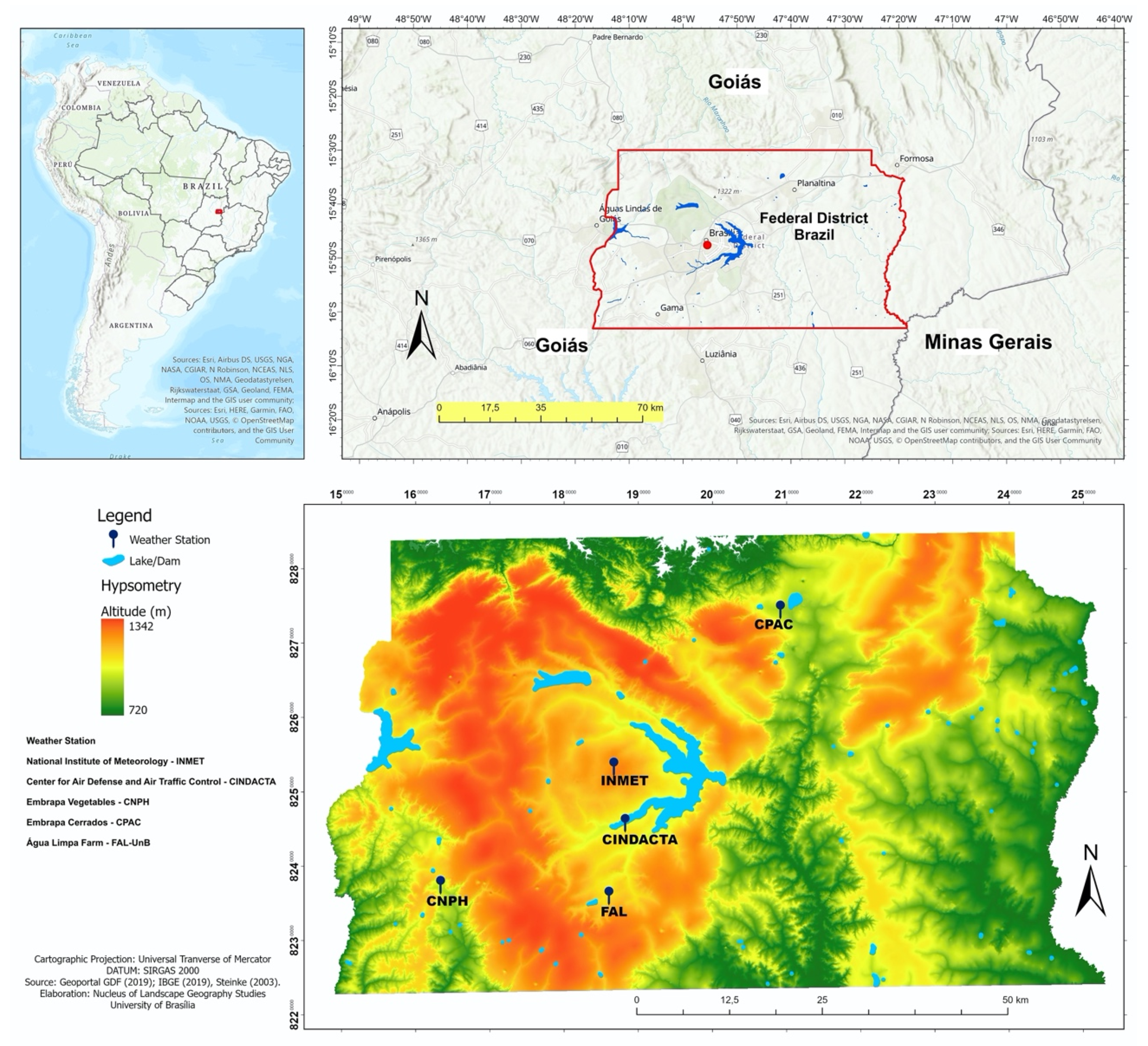
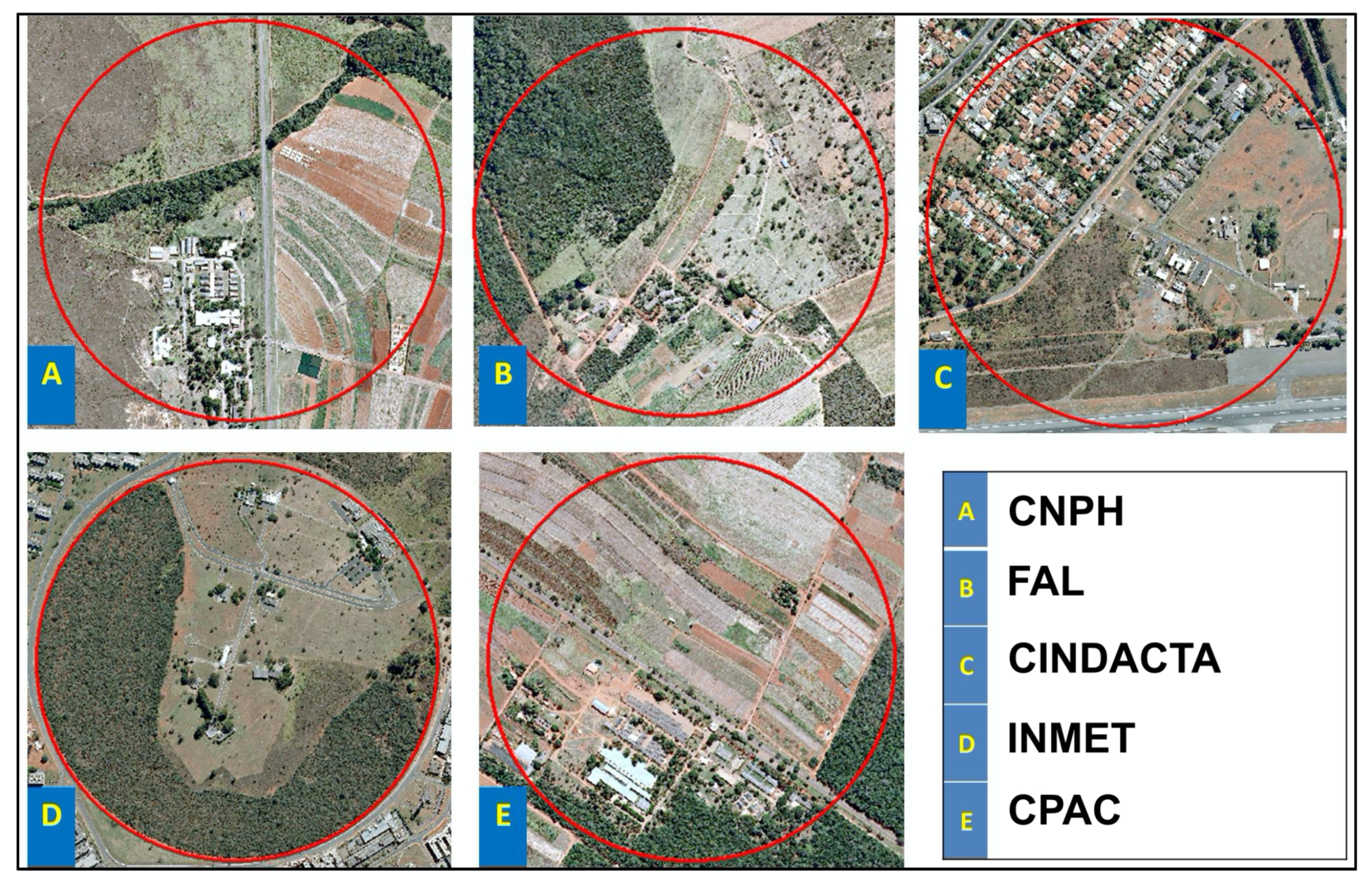
2. Materials and Methods
Data Set Analysis
- T = total number of groups with identical symbols.
- H0 = there is no trend;
- H1 = there is a trend.
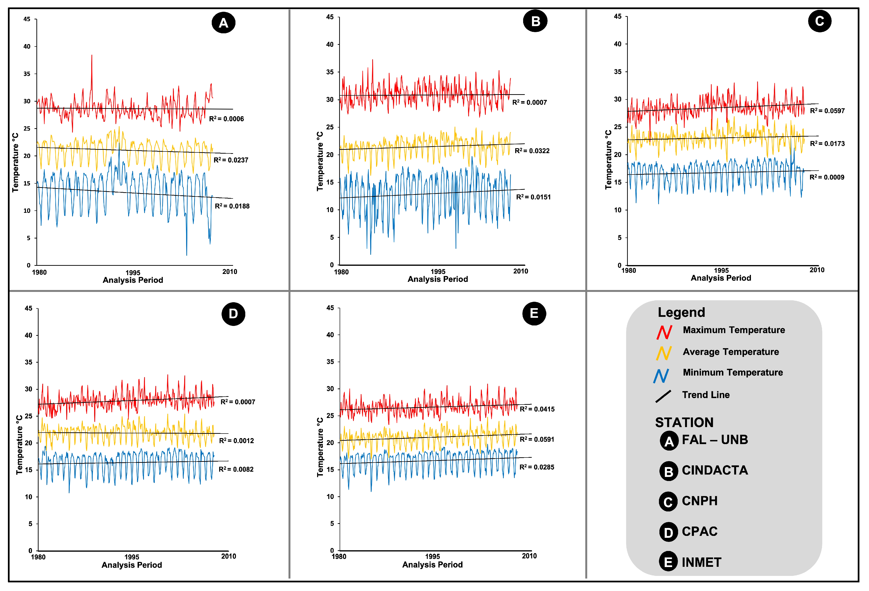
3. Results
4. Discussion
5. Conclusions
Author Contributions
Funding
Conflicts of Interest
References
- Jones, P.D.; Moberg, A. Hemispheric and large-scale surface air temperature variations: An extensive revision and an update to 2001. Boston J. Clim. 2003, 16, 206–223. [Google Scholar] [CrossRef] [Green Version]
- Stewart, I.D.; Oke, T.R. Methodological concerns surrounding the classification of urban and rural climate stations to define urban heat island magnitude. In Proceedings of the Sixth International Conference on Urban Climate, Goteborg, Sweeden, 12–16 July 2006; pp. 431–444. [Google Scholar]
- Shitara, H. Effects of buildings upon the winter temperature in Hiroshima city. Geogr. Rev. 1957, 30, 468–482. (In Japanese) [Google Scholar] [CrossRef] [Green Version]
- Louw, W.J.; Meyer, J.A. Near-surface nocturnal winter temperatures in Pretoria. Notos 1965, 14, 49–65. [Google Scholar]
- Chandler, T.J. The Climate of London; Hutchinson: London, UK, 1965; p. 292. [Google Scholar]
- Ludwig, F.L. Urban Temperature Fields. Urban Climates; Technical Note n.108; WMO: Geneva, Switzerland, 1970; pp. 80–107. [Google Scholar]
- Sharon, D.; Koplowitz, R. Observations of the Heat Island of a Small Town; Meteorologische Rundschau: Stuttgart, Germany, 1972; Volume 25, pp. 143–146. [Google Scholar]
- Okoola, R.E. The Nairobi heat island.Kenya. J. Sci. Technol. 1980, 1A, 53–65. [Google Scholar]
- Oke, T.R. Boundary Layer Climates; Routledge: Abingdon on Thames, UK, 1987; p. 435. [Google Scholar]
- Robaa, S.M. Urban-suburban/rural differences over Greater Cairo, Egypt. Atmósfera 2003, 16, 157–171. [Google Scholar]
- Nunes da Silva, E.; Ribeiro, H. Temperature modifications in shantytown environments and thermal discomfort. Rev. Saúde Publica 2006, 40, 663–670. [Google Scholar]
- Amorim, M.C.C.T.; Dubreuil, V.; Cardoso, R.D.S. Modelagem espacial da ilha de calor urbana em presidente prudente (SP)—Brasil. Rev. Bras. Climatol. 2015, 11, 29–45. [Google Scholar] [CrossRef] [Green Version]
- Skarbit, N.; Stewart, I.D.; Unger, J.; Gál, T. Employing an urban meteorological network to monitor air temperature conditions in the ‘local climate zones’ of Szeged, Hungary. Int. J. Climatol. 2017, 37 (Suppl. S1), 582–596. [Google Scholar] [CrossRef]
- Amorim, M.C.C.T. Intensidade e forma da ilha de calor urbana em Presidente Prudente/SP. Geosul (UFSC) 2005, 20, 65–82. [Google Scholar]
- Amorim, M.C.C.T. Climatologia e gestão do espaço urbano. Mercator (Fortaleza. Online) 2010, 9, 71–90. [Google Scholar]
- Mendonça, F.; Dubreuil, V. L’étude du climat urbain au Brésil: Etat actuel et contribution de la télédétection. In Environnement et Télédétection au Brésil; Presses Universitaires de Rennes: Rennes, France, 2002; pp. 135–146. [Google Scholar]
- Amorim, M.C.C.T.; Dubreuil, V.; Quenol, H.; Sant’anna, J.L. Características das ilhas de calor em cidades de porte médio: Exemplos de Presidente Prudente (Brasil) e Rennes (França). Confins [Online] 2009, 7, 16. [Google Scholar] [CrossRef]
- Amorim, M.C.C.T. O Clima Urbano de Presidente Prudente/SP. São Paulo. Ph.D. Thesis, Faculty of Philosophy, Letters and Human Sciences, University of Sao Paulo, Sao Paulo, Brazil, 2000. [Google Scholar]
- Stewart, I.D.; Oke, T.R. Newly developed “thermal climate zones” for defining and measuring urban heat island magnitude in the canopy layer. In Proceedings of the Preprints, T.R. Oke Symposium & Eighth Symposium on Urban Environment, Phoenix, AZ, USA, 10 January 2009; pp. 11–15. [Google Scholar]
- Oke, T.R. Initial Guidance to Obtain Representative Meteorological Observations at Urban Sites; IOM Report 81, WMO/TD. No. 1250; World Meteorological Organization: Geneva, Switzerland, 2006; Available online: http://www.wmo.int/pages/prog/www/IMOP/publications/IOM-81/-UrbanMetObs.pdf (accessed on 15 July 2020).
- Hansen, J.; Lebedeff, S. Global trends of measured surface air temperature. J. Geophys. Res. 1987, 92, 13345–13372. [Google Scholar] [CrossRef] [Green Version]
- Back, A.J. Aplicação de análise estatística para identificação de tendências climáticas. Pesq. Agropec. Bras. 2001, 36, 717–726. [Google Scholar] [CrossRef]
- Munuzzi, R.B.; Caramori, P.H. Tendência climática sazonal e anual da quantidade de chuva no estado do Paraná. Rev. Bras. Meteorol. 2010, 25, 237–246. [Google Scholar]
- Silva, H.J.F. Análise de Tendência e Caracterização Sazonal e Interanual da Evapotranspiração de Referência Para o Sudoeste da Amazônia Brasileira: Acre, Brasil. Master’s Thesis, Federal University of Rio Grande do Norte, Natal, Brazil, 2010. [Google Scholar]
- Dos Santos Gomes, A.C.; da Silva Costa, M.; Coutinho, M.D.L.; do Vale, R.S.; dos Santos, M.S.; da Silva, J.T.; Fitzjarrald, D.R. Análise estatística das tendências de elevação nas séries de temperatura média máxima na amazônia central: Estudo de caso para a região do oeste do Pará. Rev. Bras. Climatol. 2015, 11, 17. [Google Scholar]
- Chattopadhyay, S.; Edwards, D.R. Long-term trend analysis of precipitation and air temperature for Kentucky, United States. Climate 2016, 4, 10. [Google Scholar] [CrossRef]
- Ray, L.K.; Goel, N.K.; Arora, M. Trend analysis and change point detection of temperature over parts of India. Theor. Appl. Climatol. 2019, 138, 153–167. [Google Scholar] [CrossRef]
- Livada, I.; Synnefa, A.; Haddad, S.; Paolini, R.; Garshasbi, S.; Ulpiani, G.; Fiorito, F.; Vassilakopoulou, K.; Osmond, P.; Santamouris, M. Time series analysis of ambient air-temperature during the period 1970–2016 over Sydney, Australia. Sci. Total Environ. 2019, 648, 1627–1638. [Google Scholar] [CrossRef]
- Higashino, M.; Stefan, H.G. Trends and correlations in recent air temperature and precipitation observations across Japan (1906–2005). Theor. Appl. Climatol. 2020, 140, 517–531. [Google Scholar] [CrossRef]
- Ribeiro, M.d.S.B. Variação Climática no Distrito Federal: Componentes e Perspectivas Para o Planejamento Urbano. Master’s Thesis, Faculty of Arquitecture and Urbanism, University of Brasilia, Brasilia, Brasil, 2000. [Google Scholar]
- De Mello Baptista, G.M. Estudo multitemporal do fenômeno ilhas de calor no Distrito Federal. Medio Ambient. 2002, 2, 3–17. [Google Scholar]
- Steinke, E.T.; de Andrade Souza, G.; Saito, C.H. Análise da variabiliade da temperatura do ar e da precipitação no Distrito Federal no período de 1965/2003 e sua relação com uma possível alteração climática. Rev. Bras. Climatol. 2005, 1, 131–145. [Google Scholar]
- Codeplan. Atlas do Distrito Federal; Codeplan: Brasilia, Brazil, 1984; Volume II. [Google Scholar]
- Semarh. Mapa Ambiental do Distrito Federal; Semarh: Brasília, Brazil, 2000; Scale: 1:100.000. CD-ROM.
- Steinke, V.A. Uso Integrado de Dados Digitais Morfométricos (Altimetria e Sistema de Drenagem) na Definição de Unidades Geomorfológicas no Distrito Federal, Brasília. Master’s Thesis, University of Brasilia, Brasilia, Brazil, 2003. 101 f. [Google Scholar]
- Steinke, V.A.; Sano, E.E. Semi-automatic identification, gis-based morphometry of geomorphic features of federal district of brazil. Rev. Bras. Geomorfol. 2011, 12, 3–9. [Google Scholar] [CrossRef]
- Barros, J.R. A chuva no Distrito Federal: O Regime e as Excepcionalidades do Ritmo. Master’s Thesis, State Paulista University, Rio Claro, Brazil, 2003. 221 f. [Google Scholar]
- Barros, J.R.; Zavattini, J.A.; Pitton, S. Doenças respiratórias e tipos de tempo no Distrito Federal. In Saberes e Fazeres Geográficos; Gerardi, L.H.O., Ferreira, E.R., Eds.; UNESP/IGCE e AGETEO: Rio Claro, Brazil, 2008; Volume 1, pp. 9–23. [Google Scholar]
- Steinke, E.T. Considerações Sobre Variabilidade e Mudança Climática no Distrito Federal, suas Repercussões nos Recursos Hídricos e Informação ao Grande Público. Ph.D. Thesis, University of Brasilia, Brasilia, Brazil, 2004. 201 f. [Google Scholar]
- Morettin, P.A.; Toloi, C.M.C. Análise de Séries Temporais, 2nd ed.; E. Blucher: Sao Paulo, Brazil, 2006. [Google Scholar]
- Neves, A.I.L.R.N.C.N. Detecção de Tendências no Padrão Temporal de Variáveis Hidrológicas. Aplicação à Precipitação a Diferentes Escalas Temporais. Covilhã. Master’s Thesis, University of Beira Interior, Covilha, Portugal, 2012. 192 f. [Google Scholar]
- Sonali, P.; Nagesh, K.D. Review of trend detection methods and their application to detect temperature changes in India. J. Hydrol. 2013, 476, 212–227. [Google Scholar] [CrossRef]
- Horos, M.T.; Dalfes, N.; Karaca, M.; Yenigün, O. A comparative assessment of different methods for detecting inhomogeneities in Turkish temperature data set. Int. J. Climatol. 1998, 18, 561–578. [Google Scholar] [CrossRef]
- Tröger, F.H.; Pante, A.R. Análise de estacionariedade em séries de vazões naturais médias anuais de estações da bacia do rio Tapajós. In Proceedings of the Simpósio Brasileiro De Recursos Hídricos, Campo Grande, Brazil, 22–26 November 2009; Anais Campo Grande: ABRH, 2009. Available online: https://www.abrhidro.org.br/SGCv3/publicacao.php?PUB=3&ID=110&SUMARIO=1792 (accessed on 15 July 2020).
- Coelho, M.; Fernandes, C.; Scapulatempo, V.; Detzel, D.H.M.; Mannich, M. Statistical validity of water quality time series in urban watersheds. RBRH 2017, 22, e51. [Google Scholar] [CrossRef]
- Rao, A.R.; Humed, K.H. Frequency analysis of Upper Cauvery flood data by L-moments. Water Resour. Manag. 1994, 8, 83–201. [Google Scholar] [CrossRef]
- Rao, A.R.; Humed, K.H. Flood Frequency Analysis; CRC Press: Boca Raton, FL, USA, 2000. [Google Scholar]
- Cox, D.R.; Stuart, A. Some Quick Tests for Trend in Location and Dispersion; Biometrika: London, UK, 1965; Volume 42, pp. 80–95. [Google Scholar]
- Morettin, P.A.; Toloi, C.M.C. Modelos de Função de Transferência; ABE: Sao Paulo, Brazil, 1989.
- McCuen, R.H. Modeling Hydrologic Change: Statistical Methods; Lewis Publishers: Boca Raton, FL, USA; London, UK; New York, NY, USA; Washington, DC, USA, 2003. [Google Scholar]
- Niedzielski, T.; Kosek, W. A required data span to detect sea level rise. In Advances in Marine Navigation and Safety of Sea Transportation; Weintrit, A., Ed.; Gdynia Maritime University: Gdynia, Poland, 2007; pp. 367–371. [Google Scholar]
- Mann, H.B. Non-parametric test against trend. Econometrica 1945, 13, 245–259. [Google Scholar] [CrossRef]
- Kendall, M.G. Rank Correlation Methods, 4th ed.; Charles Griffin: London, UK, 1975. [Google Scholar]
- Gilbert, R.O. Statistical Methods for Environmental Pollution Monitoring; Van Nostrand Reinhold: New York, NY, USA, 1987. [Google Scholar]
- Partal, T.; Kahya, E. Trend analysis in Turkish precipitation data. Hydrol. Process 2006, 20, 2011–2026. [Google Scholar] [CrossRef]
- Jaagus, J. Climatic changes in Estonia during the second half of the 20th century in relationship with changes in large-scale atmospheric circulation. Theor. Appl. Climatol. 2006, 83, 77–88. [Google Scholar] [CrossRef]
- Modarres, R.; da Silva, V.P.R. Rainfall trends in arid and semi-arid regions of Iran. J. Arid. Environ. 2007, 70, 344–355. [Google Scholar] [CrossRef]
- Tabari, H.; Marofi, S.; Ahmadi, M. Long-term variations of water quality parameters in the Maroon River, Iran. Environ. Monitor. Assess. 2010, 177, 273–287. [Google Scholar] [CrossRef] [PubMed]
- Tabari, H.; Marofi, S.; Hosseinzadeh Talaee, P.; Mohammadi, K. Trend analysis of reference evapotranspiration in the western half of Iran. Agric. For. Meteorol. 2011, 151, 128–136. [Google Scholar] [CrossRef]
- Yue, S.; Pilon, P.; Phinney, B.; Cavadias, G. The influence of autocorrelation on the ability to detect trend in hydrological series. Hydrol. Process. 2002, 16, 1807–1829. [Google Scholar] [CrossRef]
- Gomes, F.P. Curso de Estatística Experimental, 15th ed.; Esalq. SP: Piracicaba, Brazil, 2009. [Google Scholar]
- Triola, M. Minitab Student Laboratory Manual and Workbook, 10th ed.; Addison-Wesley: Boston, MA, USA, 2006. [Google Scholar]
- World Meteorological Organization (WMO). Guide to Meteorological Instruments and Methods of Observation WMO-No. 8; WMO: Geneva, Switzerland, 2018; Available online: https://library.wmo.int/index.php?lvl=notice_display&id=12407#.XvesWGT0n6Y (accessed on 15 July 2020).
- Peña Quiñones, A.J.; Chaves Cordoba, B.; Salazar Gutierrez, M.R.; Keller, M.; Hoogenboom, G. Radius of influence of air temperature from automated weather stations installed in complex terrain. Theor. Appl. Climatol. 2019, 137, 1957–1973. [Google Scholar] [CrossRef]
- Landsberg, H.E. The Urban Climate; Academic: Orlando, FL, USA, 1981; p. 275. [Google Scholar]
- Gartland, L. Ilhas de Calor: Como Mitigar Zonas de Calor em Áreas Urbanas; Translated by Silvia Helena Gonçalves; Oficina de Textos: Sao Paulo, Brazil, 2010. [Google Scholar]
- Ruth, M.; Baklanov, A. Urban climate science, planning, policy and investment challenges. Urban Clim. 2012, 1, 1–3. [Google Scholar] [CrossRef]
- De Figueiredo Monteiro, C.A. Teoria e Clima Urbano; IGEO/USP: Sao Paulo, Brazil, 1976. [Google Scholar]


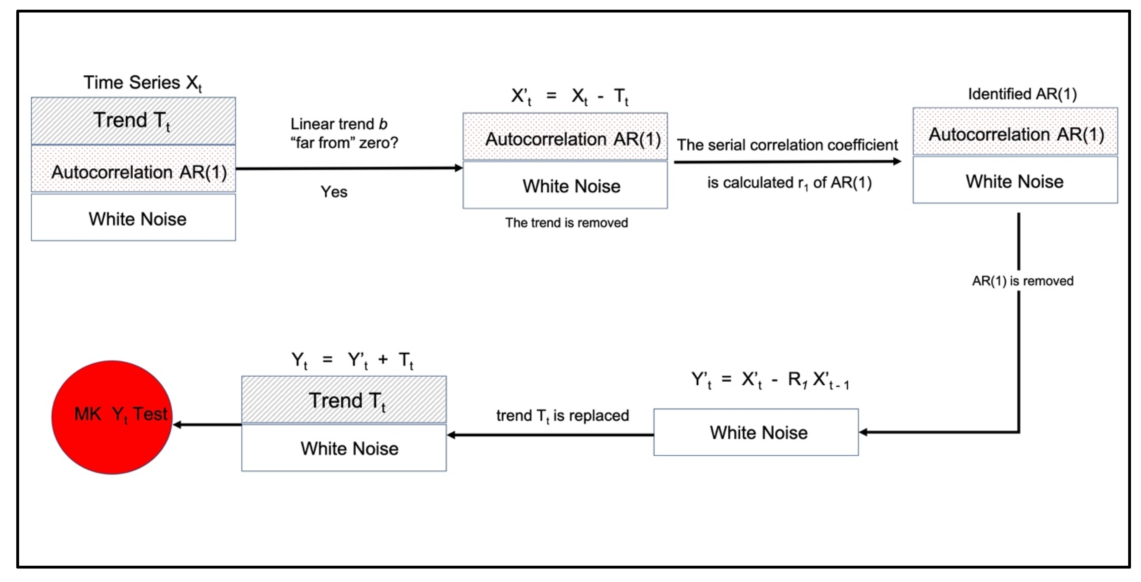
| Step 1. | The linear trend b of series Xt estimated by the Theil–Sen method is calculated. If b is “close” to zero, then it is assumed that there is no trend and the procedure ends. |
| Step 2 | If b is not “close” to zero, a linear trend Tt in series Xt is assumed and the trend is removed from it: X’t = Xt − Tt = Xt − bt |
| Step 3 | Considering the autoregressive model AR (1), the serial correlation coefficient r1 of the series (without trend) X’t is calculated and the autocorrelation AR (1) is removed from it: Y’t = X’t − r1 X’t−1 |
| Step 4 | Series Y’t, which is now “clean”, without a trend Tt or AR (1) autocorrelation, is “pasted” to the trend to be identified by the Mann–Kendall test: Yt = Y’t + Tt In this way, Yt preserves its true trend and is not influenced by the effects of autocorrelation. |
| Step 5: | The Mann–Kendall test is applied to series Yt. |
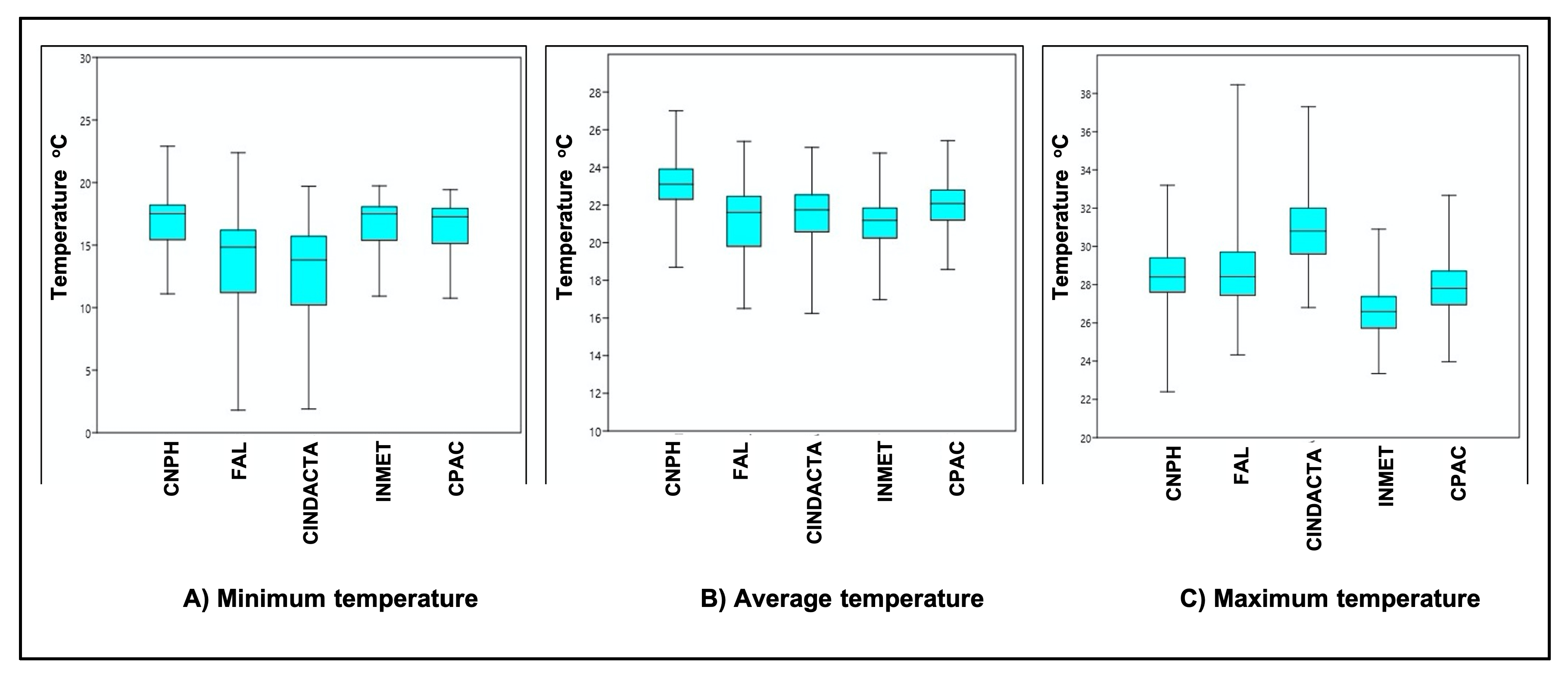
| Maximum temperature | CNPH | FAL | CINDACTA | INMET | CPAC | |
| N | 372 | 372 | 372 | 372 | 372 | |
| Min | 22.4 | 24.33 | 26.8 | 23.35 | 23.97 | |
| Max | 33.2 | 38.45 | 37.3 | 30.9 | 32.67 | |
| Mean | 2.850457 | 2.865693 | 3.089194 | 2.661524 | 2.789621 | |
| Std. error | 0.07870086 | 0.1066252 | 0.09394739 | 0.06954393 | 0.07500937 | |
| Variance | 2.304103 | 3.001398 | 31.774 | 1.799125 | 2.093023 | |
| Stand. Dev | 1.517927 | 1.732454 | 1.782526 | 1.341315 | 1.446728 | |
| Median | 28.4 | 28.415 | 30.8 | 26.585 | 27.8 | |
| 25th percentile | 27.6 | 27.435 | 29.6 | 25.7225 | 26.9425 | |
| 75th percentile | 29.4 | 29.7 | 32 | 27.375 | 28.7075 | |
| Skewness | 0.1657374 | 0.9238805 | 0.3261668 | 0.4618178 | 0.4384937 | |
| Kurtosis | 0.9266567 | 3.26823 | −0.1142808 | 0.3999233 | 0.6199819 | |
| Geom. mean | 28.4643 | 28.60623 | 30.84111 | 26.58194 | 27.85921 | |
| Coeff. var | 5.325207 | 6.045498 | 5.770198 | 5.039649 | 5.186111 | |
| Average temperature | CNPH | FAL | CINDACTA | INMET | CPAC | |
| N | 372 | 372 | 372 | 372 | 372 | |
| Min | 18.7 | 16.5 | 16.24403 | 16.97 | 18.58 | |
| Max | 27 | 25.375 | 25.05969 | 24.76 | 25.42 | |
| Mean | 2.305591 | 2.113223 | 21.439 | 2.102269 | 2.190777 | |
| Std. error | 0.07048884 | 0.1133258 | 0.08263705 | 0.06855809 | 0.06728182 | |
| Variance | 1.848348 | 3.390484 | 2.458398 | 1.748479 | 1.683986 | |
| Stand. dev | 13.5954 | 18.41327 | 15.67928 | 13.22301 | 12.97685 | |
| Median | 23.1 | 21.63 | 21.74049 | 21.18 | 22.075 | |
| 25th percentile | 22.3 | 19.825 | 20.57064 | 20.24 | 21.195 | |
| 75th percentile | 23.9 | 22.45 | 22.53285 | 21.84 | 22.7825 | |
| Skewness | −0.1450918 | −0.536335 | −0.603428 | −0.3672645 | −0.2616349 | |
| Kurtosis | 0.6940948 | −0.441302 | 0.127792 | 0.203304 | −0.0552102 | |
| Geom. mean | 23.01548 | 21.04918 | 21.37971 | 20.98035 | 21.86888 | |
| Coeff. var | 5.896706 | 8.713355 | 7.313438 | 6.289874 | 59.234 | |
| Minimum temperature | CNPH | FAL | CINDACTA | INMET | CPAC | |
| N | 372 | 372 | 372 | 372 | 372 | |
| Min | 11.1 | 1.8 | 1.9 | 10.92 | 10.75 | |
| Max | 22.9 | 22.38 | 19.7 | 19.73 | 19.43 | |
| Mean | 16.8628 | 13.80871 | 12.89667 | 16.75196 | 16.49371 | |
| Std. error | 0.09772559 | 0.2025824 | 0.1800133 | 0.09051469 | 0.09812114 | |
| Variance | 3.552708 | 10.83446 | 11.66573 | 3.047762 | 3.581526 | |
| Stand. dev | 1.884863 | 3.291574 | 3.415513 | 1.745784 | 1.892492 | |
| Median | 17.5 | 14.83 | 13.8 | 17.49 | 17.255 | |
| 25th percentile | 15.425 | 11.2 | 10.2 | 153.675 | 15.12 | |
| 75th percentile | 18.2 | 16.2 | 15.7 | 180.575 | 17.93 | |
| Skewness | −0.652321 | −0.686684 | −0.56908 | −0.8709872 | −0.8232476 | |
| Kurtosis | −0.2157347 | 0.048029 | −0.4952163 | −0.2862008 | −0.483233 | |
| Geom. mean | 16.75096 | 13.31522 | 12.33696 | 16.65447 | 16.37693 | |
| Coeff. var | 11.17764 | 23.83694 | 26.48369 | 10.42137 | 11.47402 |
| Test (p-Value) | Step 1 | Test (p-Value) | Step 2 | ||||
|---|---|---|---|---|---|---|---|
| Temperature | Station | Wald–Wolfowitz | Cox–Stuart | Mann–Kendall | Is There a Trend? | MK-Adjusted | Is There a Trend? |
| Minimum | CINDACTA | 2.0062 × 10⁻²⁴ | 0.057615976 | 0.017756332 | yes | 0.2510 | no |
| FAL | 1.69571 × 10⁻²³ | 0.001414448 | 0.248676166 | yes | 0.0948 | no | |
| INMET | 4.7 × 10⁻²⁹ | 0.045721123 | 1.415 × 10⁻⁷ | yes | 0.3127 | no | |
| CPAC | 0 | 0.081699116 | 0.010615543 | yes | 0.8776 | no | |
| CNPH | 7 × 10⁻³⁰ | 0.106234147 | 0.009305695 | yes | 0.1907 | no | |
| Average | CINDACTA | 2.43843 × 10⁻¹⁵ | 2.2172 × 10⁻⁶ | 0.000200051 | yes | 0.0948 | no |
| FAL | 2.25623 × 10⁻²⁰ | 3.7 × 10⁻⁹ | 0.004867564 | yes | 0.4656 | no | |
| INMET | 3.91319 × 10⁻¹³ | 0.003976863 | 2.0376 × 10⁻⁶ | yes | 0.0131 | no | |
| CPAC | 9.8304 × 10⁻¹⁷ | 0.412983814 | 0.184920311 | no | 0.1684 | no | |
| CNPH | 2.10328 × 10⁻¹¹ | 0.00072815 | 0.001942255 | yes | 0.2310 | yes | |
| Maximum | CINDACTA | 2.46062 × 10⁻¹¹ | 0.183556922 | 0.365201205 | no | 0.5374 | no |
| FAL | 5.75176 × 10⁻⁸ | 0.011371634 | 0.309852392 | yes | 0.2511 | no | |
| INMET | 3.7282 × 10⁻⁸ | 0.0002667 | 0.000222662 | yes | 0.0033 | yes | |
| CPAC | 1.53129 × 10⁻⁷ | 1.26909 × 10⁻⁵ | 4.663 × 10⁻⁷ | yes | 0.0014 | yes | |
| CNPH | 5.69459 × 10⁻⁹ | 0.000316394 | 1.68551 × 10⁻⁵ | yes | 0.0198 | yes | |
| Station | Altitude | Is There a Trend? | What Is the Trend? | Trend Percentage * | ||
|---|---|---|---|---|---|---|
| Tmax | Tav | Tmin | ||||
| CINDACTA | 1055 | yes | Increase | 0.1% | 3% | 1.5% |
| FAL | 1080 | yes | decrease | 0.2% | 2% | 1% |
| INMET | 1160 | yes | Increase | 4% | 6% | 3% |
| CPAC | 1000 | yes | Increase | 0.7% | 0.1% | 0.1% |
| CNPH | 1000 | yes | Increase | 5% | 2% | 1% |
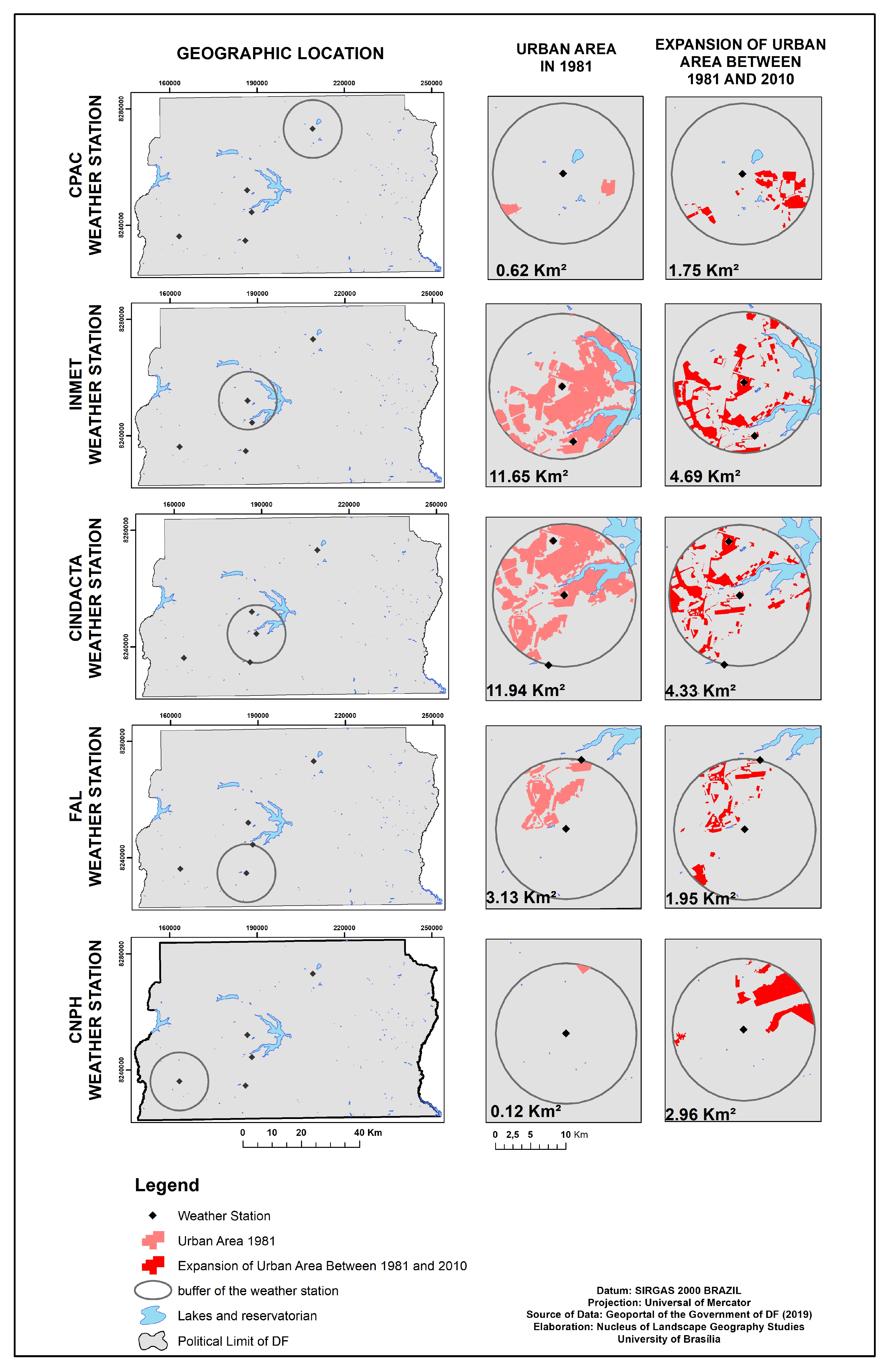
| Station | Area of Influence | Urban Area 1981 | Growth in 1981–2010 | Growth Rate | Urban Area in 2010 | |||
|---|---|---|---|---|---|---|---|---|
| Name | km2 | km2 | % | km2 | % | % | km2 | % |
| CNPH | 29 | 0.12 | 0.43 | 2.96 | 10.20 | 2330.70 | 3.08 | 10.64 |
| INMET | 29 | 11.65 | 40.17 | 4.69 | 16.17 | 40.25 | 16.34 | 56.34 |
| CPAC | 29 | 0.62 | 2.13 | 1.75 | 6.03 | 282.25 | 2.37 | 8.17 |
| CINDACTA | 29 | 11.94 | 41.17 | 4.33 | 14.93 | 36.26 | 16.27 | 56.10 |
| FAL | 29 | 3.13 | 10.79 | 1.95 | 6.72 | 62.30 | 5.08 | 17.51 |
© 2020 by the authors. Licensee MDPI, Basel, Switzerland. This article is an open access article distributed under the terms and conditions of the Creative Commons Attribution (CC BY) license (http://creativecommons.org/licenses/by/4.0/).
Share and Cite
Steinke, V.A.; Martins Palhares de Melo, L.A.; Luiz Melo, M.; Rodrigues da Franca, R.; Luna Lucena, R.; Torres Steinke, E. Trend Analysis of Air Temperature in the Federal District of Brazil: 1980–2010. Climate 2020, 8, 89. https://0-doi-org.brum.beds.ac.uk/10.3390/cli8080089
Steinke VA, Martins Palhares de Melo LA, Luiz Melo M, Rodrigues da Franca R, Luna Lucena R, Torres Steinke E. Trend Analysis of Air Temperature in the Federal District of Brazil: 1980–2010. Climate. 2020; 8(8):89. https://0-doi-org.brum.beds.ac.uk/10.3390/cli8080089
Chicago/Turabian StyleSteinke, Valdir Adilson, Luis Alberto Martins Palhares de Melo, Mamedes Luiz Melo, Rafael Rodrigues da Franca, Rebecca Luna Lucena, and Ercilia Torres Steinke. 2020. "Trend Analysis of Air Temperature in the Federal District of Brazil: 1980–2010" Climate 8, no. 8: 89. https://0-doi-org.brum.beds.ac.uk/10.3390/cli8080089