Development of a Parametric Regional Multivariate Statistical Weather Generator for Risk Assessment Studies in Areas with Limited Data Availability

Abstract

Risk analysis of water resources systems can use statistical weather generators coupled with hydrologic models to examine scenarios of extreme events caused by climate change. These require multivariate, multi-site models that mimic the spatial, temporal, and cross correlations of observed data. This study developed a statistical weather generator to facilitate bottom-up approaches to assess the impact of climate change on water resources systems for cases of limited data. While existing weather generator models have impressive features, this study suggested a simple weather generator which is straightforward to implement and can employ any distribution function for variables such as precipitation or temperature. It is based on (1) a first-order, two-state Markov chain to simulate precipitation occurrences; (2) the use of Wilks’ technique to produce correlated weather variables at multiple sites with the conservation of spatial, temporal, and cross correlations; (3) the capability to vary the statistical parameters of the weather variables. The model was applied to studies of the Diyala River basin in Iraq, which is a case with limited observed records. Results show that it exhibits high values (e.g., over 0.95) for the Nash–Sutcliffe and Kling–Gupta metric tests, preserves the statistical properties of the observed variables, and conserves the spatial, temporal, and cross correlations among the weather variables in the meteorological stations.

1. Introduction

Climate change impacts are of increasing concern to hydrologists who assess risks in the management of water resources systems. Their models of climate scenarios for extreme events can be derived from global climate models (GCMs), stochastic-statistical weather generators (SWGs), or a combination. Although they have their own advantages, some argue that the GCM scenarios are inadequate and limit decision-making options because they represent only specific scenarios for climatic variability and have large uncertainties [1,2,3,4,5,6]. On the other hand, others think that SWGs can produce a wide range of scenarios to study system responses and provide more insights about the system performance under climate change [7,8,9,10]. The drawbacks of the SWGs are that they have a stochastic-basis and cannot provide future change insights. Therefore, the SWGs and GCMs have been linked to generate forecasting scenarios and to assign a probability of each SWG scenario by fitting a distribution to the GCM outcomes [11,12,13]. In this way, SWGs can then be used to generate probabilistic synthetic scenarios with the aid of the GCM information and which are statistically similar to observed data and used to investigate which climate states cause system failure [4,14,15,16,17,18,19,20,21,22,23]. Where historic records are limited, synthetic weather sequences based on SWGs are especially suitable [24].

Given the previous work, the main objective of this paper is to develop a SWG that can be used in a bottom-up approach to generate daily synthetic scenarios to evaluate the impacts of long-term climate change on system performance and suggest robust adaptations to cope with anticipated negative impacts that will be examined in a follow up study. Emphasis is placed on areas with low data availability, and the model is demonstrated for Diyala River basin in Iraq for the four historic weather variables (e.g., precipitation, maximum and minimum temperatures, and wind speed magnitude) with daily time steps from 1948 to 2006.

2. Literature Review

Generally, SWGs can be grouped into parametric, non-parametric, and semi-parametric methods. In the parametric method, the weather variables are assumed to fit one continuous probability distribution or two combined distributions. The parameters are usually estimated from historic observations [24,25,26,27,28]. In the non-parametric method, the weather variables are resampled from historic observations using techniques such as empirical distributions, neural networks, and maximum entropy bootstrap [29,30,31,32]. The semi-parametric method is a mixture between parametric and non-parametric methods.

Albeit other approaches have their advantages, the parametric SWG in the bottom-up approach is preferable because the parameters can be altered to simulate different weather scenarios and facilitate climate change studies [16]. Verdin et al., [15], Furrer and Katz [18], Buishand and Brandsma [33], Seneviratne et al., [34] noted that the non-parametric method has limitations in generating extreme events because values can only be in the range of the observations. Using only the observed sequences ignores climate change’s impacts on altering the intensities of the variables and is insufficient in assessing the future response of water resources systems because it leads to single results corresponding only to these observed sequences [22,23,25,34,35,36].

Most existing SWGs are for single sites and cannot capture the spatial and cross correlations between the variables, which are essential for generating realistic climate change scenarios. Schaake et al., [37] stated that “relationships between physically dependent variables like precipitation and temperature should be respected”. Single site SWGs can fail to capture the extreme events of the generated runoff, which are essential to develop realistic adaptation strategies to cope with flood and drought events, especially where a high runoff in one sub-basin can be offset by the low runoff in adjacent sub-basins [26,35,38].

Moreover, the misrepresentation of spatial and cross correlations (e.g., correlations between the precipitation and temperature) leads to biased generated streamflows as this correlation determines the water availability for evapotranspiration and snowmelt [32,39,40]. Therefore, SWGs should capture the characteristics of each site and the spatial dependence among them.

Recently, multi-site and multi-variable SWGs have been developed using different approaches. Steinschneider and Brown, [4] developed a semi-parametric model using a k-nearest-neighbor resampling scheme to simulate multiple spatially distributed variables using wavelet decomposition and autoregressive model to account for low-frequency oscillations. They used a Markov chain of first-order with three states to identify the precipitation states (e.g., dry, wet, and extremely wet). This model had difficulty in preserving the weather statistics besides the cross correlation. Additionally, it is not clear how to diagnose the differences between the precipitation states (e.g., wet and extremely wet).

Srivastav and Simonovic, [32] developed a non-parametric model using the maximum entropy bootstrap technique to capture the time-dependent structure and statistical characteristics. They used an orthogonal transformation to capture the spatial correlations. Even though the model preserves the historical characteristics, Verdin et al., [15] and Chen et al., [40] showed that the maximum entropy bootstrap technique is limited to the historical data range leading to inadequacy in climate change studies. It is difficult to employ this model to create different climate scenarios through variations of parameters.

Li and Babovic, [41] proposed a two-stage parametric model using an empirical copula to generate spatial distribution templates. Then, they developed a rank ordering technique that depended on historic data ranks with an empirical copula technique to preserve the correlations between the variables. The model preserves correlations between the variables and sites but is limited to the historic record length. For example, the model cannot generate more than 30 years of simulation if the historic observations are 30 years. Therefore, the model is not useful in areas with limited data length as an insufficient projection length may lead to wrong conclusions in risk assessment studies [42,43].

Verdin et al., [15] presented a model using a Bayesian hierarchical technique. The precipitation amounts are modeled using gamma distributions and maximum and minimum temperatures are modeled using a normal distribution. The statistical coefficients within them are modeled as spatial Gaussian processes to account for the correlations. Besides the complexity of model structure, the model has difficulty in preserving the statistical properties of the variables (especially the standard deviation of the minimum temperature is extremely underestimated by the model). Additionally, the model underestimates the spatial correlation between the variables. Furthermore, their results do not demonstrate the model’s ability to preserve the cross correlation between the variables as well as the temporal correlation.

3. Model Description

The goal here is to develop a parametric regional weather generator (PR-WG) to generate daily stochastic weather variables that preserve their statistical parameters, such as the mean and standard deviations, as well as the spatial, temporal, and cross correlations among them. It should be easy to implement and adapt by altering the statistical parameters to generate synthetic future climate scenarios. The generated scenario must exceed the historic record length and observation range.

The novel contribution is to use a parametric approach to create a flexible model that can adapt to any continuous probability distribution. This will enable the use of the most accurate distribution for each weather variable, and the user can employ other distributions according to the data availability and scope of the study.

3.1. Precipitation States

The first step in developing the PR-WG is to establish the precipitation states. They are defined here as: wet days if the daily amounts equal or exceed 0.1 mm and dry days otherwise. This is similar to the approach by Verdin et al., [15] and Li and V. Babovic [41]. The approach is to use the first-order two-state Markov chain (FTMC), which is the most popular method to produce dry and wet precipitation occurrences. It works well in different climate types and performs as well as higher Markov chain orders [21,22].

Let S_(k,t,m) denote the precipitation state (S = 0 is a dry day and S = 1 is a wet day) at spatial location k ∈ ℕ, time index t ∈ ℕ in days, and month index m = {1,2, … 12}. The dry or wet day occurrence is obtained from the following conditional probabilities:

$$Pr (S_{(k,t,m)}=0 |S_{k,t-1,m}=0)={\kappa }_0\hspace{1em};\hspace{1em}Pr (S_{(k,t,m)}=1 |S_{k,t-1,m}=0)=1-{\kappa }_0$$

(1)

$$Pr (S_{(k,t,m)}=1 |S_{k,t-1,m}=1)={\kappa }_1\hspace{1em};\hspace{1em}Pr (S_{(k,t,m)}=0 |S_{k,t-1,m}=1)=1-{\kappa }_1$$

(2)

where, ${\kappa }_0$ is the probability of a dry day following a dry day, and ${\kappa }_1$ is the probability of a wet day following a wet day. These probabilities were estimated from the daily historical precipitation observations for each month.

3.2. Precipitation Amount

Precipitation amounts were calculated by using the joint probability distribution between the occurrence and amount. For example, once a wet day is predicted from the FTMC, the precipitation amount is calculated. A skewed normal distribution (SN) was selected because it was recommended by other researchers and estimates the daily precipitation amount better than other distributions such as exponential, gamma, Weibull, mixed-exponential, and generalized Pareto in capturing the mean, standard deviation, and extreme values [20,21,36,44,45].

Let P denote the precipitation amount in mm/day and ${\mathsf{𝕝}}_{\mathsf{\Psi }}$ denote the indicator of precipitation state condition ψ. P returns to a value obtained implicitly from Equation (4) [46] if the condition ψ holds (${\mathsf{𝕝}}_{\left[S=1\right]}$) and returns to zero otherwise $\left({\mathsf{𝕝}}_{\left[S=0\right]}\right)$, as follows:

$$P_{\left(k,t,m\right)}=\{\begin{array}{c} SN \left({\mu }_P, {\sigma }_P, {\gamma }_P\right) for {\mathsf{𝕝}}_{\left[S\left(k,t,m\right)=1\right]}\\ 0 for {\mathsf{𝕝}}_{\left[S\left(k,t,m\right)=0\right]}\end{array}$$

(3)

$${\theta }_{\left(k,t,m\right)}=\frac{6}{{\gamma }_{p\left(k,m\right)}} \left\{ {\left[ \frac{{\gamma }_{p\left(k,m\right)}}{2} \left(\frac{P_{\left(k,t,m\right)}-{\mu }_{p\left(k,m\right)}}{{\sigma }_{p\left(k,m\right)}}\right)+1\right]}^{\frac{1}{3}}-1\right\}+\frac{{\gamma }_{p\left(k,m\right)}}{6}$$

(4)

where θ is the matrix of the standard normal deviates θ ~ N(0,1) ϵ ℝ, and µ_p, σ_p, and γ_p, are the mean, standard deviation, and skew coefficient of the precipitation for month m. The values of the parameters µ_p, σ_p, and γ_p were estimated from the daily historical observations using the method of maximum likelihood estimation (MLE).

3.3. Maximum and Minimum Air Temperature

The maximum and minimum daily air temperatures are usually modeled by the normal distribution (N) [47,48]. Let T_X and T_N denote the maximum and minimum daily air temperature in °C, respectively. In which, T_X is (and T_N) is:

$$T_{X\left(k\right)}~ N\left({\mu }_{X\left(k\right)}, {\sigma }_{X\left(k\right)}\right)$$

(5)

where μ_X and σ_X are the mean and standard deviation of T_X, respectively. Solving Equation (5) for each month m according to ${\mathsf{𝕝}}_{\mathsf{\Psi }}$ (to account for precipitation state effects), T_x and T_N can be computed as:

$$T_{X\left(k,t,m\right)}={\mu }_{x0\left(k,m\right)}+{\sigma }_{X0\left(k,m\right)}\times {\mathsf{𝕝}}_{\left(k,t,m\right)}\hspace{1em}for\hspace{1em}{\mathsf{𝕝}}_{\left[S\left(k,t,m\right)=0\right]}$$

(6)

$$T_{X\left(k,t,m\right)}={\mu }_{\mu x1\left(k,m\right)}+{\sigma }_{X1\left(k,m\right)}\times {\mathsf{𝕝}}_{\left(k,t,m\right)}\hspace{1em}for\hspace{1em}{\mathsf{𝕝}}_{\left[S\left(k,t,m\right)=1\right]}$$

(7)

$$T_{N\left(k,t,m\right)}={\mu }_{\mu N0\left(k,m\right)}+{\sigma }_{N0\left(k,m\right)}\times {\delta }_{\left(k,t,m\right)}\hspace{1em}for\hspace{1em}{\mathsf{𝕝}}_{\left[S\left(k,t,m\right)=0\right]}$$

(8)

$$T_{N\left(k,t,m\right)}={\mu }_{\mu N1\left(k,m\right)}+{\sigma }_{N1\left(k,m\right)}\times {\delta }_{\left(k,t,m\right)}\hspace{1em}for\hspace{1em}{\mathsf{𝕝}}_{\left[S\left(k,t,m\right)=1\right]}$$

(9)

where, μ_X0, μ_X1, μ_N0, μ_N1, σ_X0, σ_X1, σ_N0, and σ_N1 are the monthly mean and standard deviation for the maximum and minimum air temperature (°C/day) for S = 0 and 1, respectively, and ʋ and δ are the matrices of standard normal deviates, such that ʋ and δ ~ N (0,1) ϵ ℝ. The parameter values of Equations (6)–(9) were estimated from the historic observations using MLEs.

3.4. Wind Speed Magnitude

Ref. [49] showed that the most accurate function to simulate the daily wind speed magnitude (WS) is Weibull with three and two parameters, respectively, followed by gamma. Given the condition that wind speed is affected by precipitation states and amounts [50], the selected distribution must be decomposed into the same distribution type. As the Weibull distribution cannot be decomposed into two Weibulls (although gamma can be [51]), wind speed magnitude was modeled by the gamma distribution (GM) in this study. Let WS denote the daily wind speed magnitude (m/s) for k locations, as follows:

$${\mathrm{WS}}_{\left(k\right)}~ \mathrm{GM} \left({\alpha }_{\left(k\right)}, {\beta }_{\left(k\right)}\right)$$

(10)

where α and β are the shape and scale parameters, respectively. Similarly for the temperature, the WS for each month m, according to ${\mathsf{𝕝}}_{\mathsf{\Psi }}$, was estimated implicitly from the following equations:

$${\lambda }_{\left(k,t,m\right)}=\frac{{\beta }_{0\left(k,m\right)}{}^{-{\alpha }_{0\left(k,m\right)}}}{\mathsf{\Gamma } \left({\alpha }_{0\left(k,m\right)}\right)} {{\displaystyle \int }}_0^{{\mathrm{WS}}_{\left(k,t,m\right)}} h^{{\alpha }_{0\left(k,m\right)}-1} ex{p}^{-h/{\beta }_{0\left(k,m\right)}} dh\hspace{1em}for\hspace{1em}{\mathsf{𝕝}}_{\left[S\left(k,t,m\right)=0\right]}$$

(11)

$${\lambda }_{\left(k,t,m\right)}=\frac{{\beta }_{1\left(k,m\right)}{}^{-{\alpha }_{0\left(k,m\right)}}}{\mathsf{\Gamma } \left({\alpha }_{1\left(k,m\right)}\right)} {{\displaystyle \int }}_0^{{\mathrm{WS}}_{\left(k,t,m\right)}} h^{{\alpha }_{1\left(k,m\right)}-1} ex{p}^{-h/{\beta }_{1\left(k,m\right)}} dh\hspace{1em}for\hspace{1em}{\mathsf{𝕝}}_{\left[S\left(k,t,m\right)=1\right]}$$

(12)

where α₀, α₁, β₀, and β₁ are the shape and scale parameters for S = 0 and 1, respectively, for each month m, h is an independent parameter, and λ is the cumulative probability, which is distributed uniformly—λ~ U [0, 1], ϵ ℝ. The shape and scale parameters were estimated from the historic observations using MLEs.

4. Model Implementation

The parametric SWG should conserve the spatial, temporal, and cross correlations of the historic observations of the four weather variables. The concept is to study the behavior of the variates θ, ʋ, δ, and λ, hereafter referred to as anomalies. The correlations between those anomalies should be identified so the generated weather values are statistically similar to the observed values and conserve spatial, temporal, and cross correlations. The implementation of the PR-WG consists of two stages, namely preprocessing and postprocessing, as shown in Figure 1.

4.1. Preprocessing: Parameter Estimation and Matrix Preparation

In order to specify the wet and dry occurrences, a random uniform variate y ~U(0, 1) must be drawn and compared with the transition probabilities obtained from Equations (1) and (2). For multi-site precipitation, the anomalies (referred to as Y ϵ ℝ) that identify the states in k locations must be correlated so that the generated states S are correlated to the historic observations. Wilks’ method was selected to generate correlated anomalies Y~ N(0,1) at multiple sites. It is simple and more efficient than hidden Markov and k-nearest neighbor methods [52], accurate in generating the correlations of monthly interstations [53], and the most cited method compared to other approaches [54].

Assume S (1,m) and S (2,m) are the precipitation states on month m at sites k = 1 and k = 2. To generate realistic sequences of the precipitation states at these two sites, the correlation (ω) between their corresponding anomalies Y, ω_(1,2) = corr (Y_(1,m), Y_(2,m)) must be computed. The parameter ω was determined by generating different sets of Ý at the two sites with different arbitrary correlation values {ώ₁, ώ₂, …}, ώ₁ =corr (Ý _(1,m), Ý _(2,m)), identifying the precipitation states at the two locations Ś₁ and Ś₂, and calculating the corresponding correlation {έ₁, έ₂, …}, έ_1(1,2) = corr (Ś_(1,m), Ś _(2,m)). Then, a regression line between έ and ώ sets was fitted to identify the relationship between them. Using this regression equation with the observed precipitation state correlation ξ, the parameter ω can then be found. A synthetic example is shown in Figure 2a, in which selecting a 0.858 correlation between the pair anomalies (ω) will produce 0.785 correlation between the pair states (ξ) at the two locations.

The process should be repeated for each station pair and lead to the number of realizations of k (k-1)/2 and be repeated for each month m to create the anomalies matrix ω_s ∈ ℝ. The ω_s matrix is then used to develop Y that produces correlated precipitation states in k locations for month m, using the multivariate normal distribution as follows,

$$Y=f \left({\mu }_y, \mathsf{\Sigma }\right)=\frac{1}{\sqrt{\mathsf{\Sigma } {\left(2\pi \right)}^d}}\exp \left(-\frac{1}{2} \left(y-{\mu }_y\right) {\mathsf{\Sigma }}^{-1} \left(y-{\mu }_y\right)\right)$$

(13)

The variable µ_y denotes the 1-D mean vector for the anomalies Y, Σ denotes the covariance matrix, and d is an independent parameter. In this case, µ = [0, 0, …, 0]_k×1 and the variance is 1, so the covariance matrix Σ_s becomes the correlation matrix ω_s.

The matrix ω_s must be a positive-definite matrix (e.g., the matrix is symmetric and all its eigenvalues are positive) to be implemented in Equation (13). Since the elements of ω_s were calculated empirically, ω_s is usually a non-positive matrix. Comparing to the work of others, the most precise method to obtain a positive-definite matrix is the iterative spectral with Dykstra’s correction (ISDC) [55], as follows:

1)

Assume ${\omega }_i= \omega$, $\Delta {\Omega }_i=0$, and $i=1$, in which ω is a non-positive-definite correlation matrix.

2)

Let $R_i={\omega }_i-\Delta {\Omega }_i$.

3)

Find $L_i$, and ${\Omega }_i$, such that $R_i={\Omega }_{i }{L}_i {\Omega }_i^T$.

4)

Replace the negative eigenvalues of $L_i$ by a small positive value to construct $L_i^{+}$.

5)

Set ${\omega }_{i+1}={\Omega }_{i }{L}_i^{+} {\Omega }_i^T$ and ${\Delta \Omega }_{i+1}={\omega }_{i+1}- R_i$. Then, replace all ${\omega }_{i+1}$ diagonal elements with 1.

6)

Test whether ${\omega }_{i+1}$ is a positive-defined matrix or not. If not, repeat the steps from two to six by making $i=i+1$ and ${\omega }_i={\omega }_{i-1}$.

After generating the matrix S at k and m, the next step is to simulate the weather variables (e.g., P, T_X, T_N and WS). The idea here is to examine the anomalies of these variables and generate the weather variables with the same observation properties. To account for all the spatial and cross correlation between the variables, their anomalies (θ, ʋ, δ, and λ) must be correlated. The temporal correlation, identified by the Lag-1 day auto-correlations, for the T_X, T_N and WS must also be considered. Since the precipitation amount is an intermittent variable, the auto-correlation is not considered. The following procedure was suggested to achieve this purpose. First, arrange the weather variable matrix V as follows,

$$\left[\begin{array}{ccc}\begin{array}{cc}\begin{array}{c}{V}_{1,1}^1\\ V_{2,1}^1\end{array}& \begin{array}{c}{V}_{1,2}^1\\ V_{2,2}^1\end{array}\end{array}& \cdots & \begin{array}{c}{V}_{1,k}^n\\ V_{2,k}^n\end{array}\\ ⋮ ⋮& \dots & ⋮\\ \begin{array}{cc}{V}_{t,1}^1& V_{t,2}^1\end{array}& \cdots & V_{t,k}^n\end{array}\right]$$

(14)

where, V represents the observed weather variable value and n denotes the weather variable rank (P, T_X, T_N and WS), n = {1, 2, 3, 4}. The total number of the rows will be T = month days × year numbers, the columns will be K × N, and the aisle will be M. This matrix arrangement enables us to consider all the spatial and cross correlations between the weather variables. Next, extract the anomalies matrix Z ∈ ℝ from V using Equations (3) and (4) for P; Equations (6)–(9) for T_x and T_N; Equations (11) and (12) for the WS, after estimating their parameters (e.g., µ_p, σ_p, γ_p for P, μ_X0, μ_X1, σ_X0, σ_X1 for T_x, μ_N0, μ_N1, σ_N0, σ_N1 for T_N, and α₀, α₁ β₀, β₁ for the WS).

The Z matrix represents the anomalies of the weather variables and their elements have spatial, cross-, and auto-correlation magnitudes. To generate the Z matrix with the same observation properties, these correlations must be preserved. The first step done here was to estimate autoregressive model of order 1, AR(1), coefficients for the anomalies (φ_z) so that the generated variables have the observed AR(1) value (φ_v) applying Wilks’ technique. For illustration, synthetically assume that the values of μ_X0, μ_X1, σ_X0, σ_X1 are 11.72, 9.12, 3.71, 2.21 (C^o/day), respectively, and φ_v is 0.82 at station k of month m. The adopted procedure for obtaining the φ_z is as follows:

1)

Generate the standard normal random deviate set y; y ~ N (0,1).

2)

Use y with Equations (1) and (2) to identify the dry and wet days.

3)

Generate a standard normal random deviate set x; x ~ N (0,1).

4)

Apply the AR(1) of arbitrary values between –1 and 1 (e.g., φ’_z).

5)

Obtain the anomalies z by standardizing x of Step 4.

6)

Apply Equations (6) and (7) to obtain T’_X.

7)

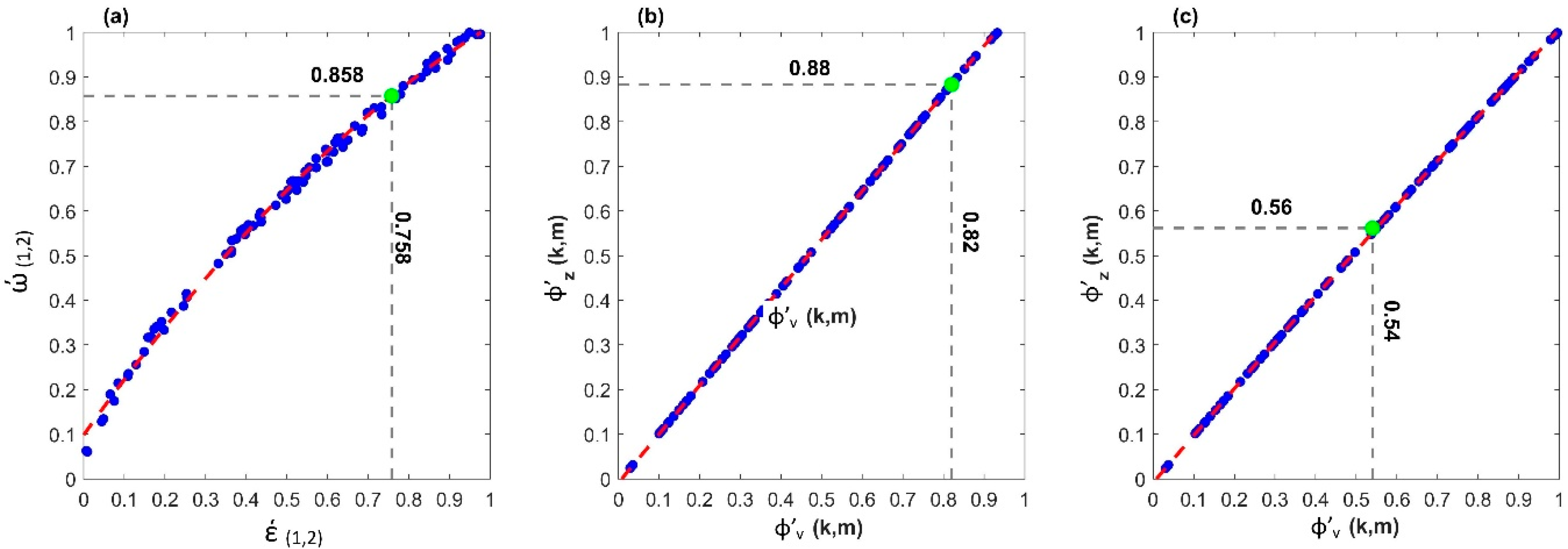
Calculate the AR (1) of T_X (e.g., φ’_v) and plot versus the φ’_z, then regress them.

8)

Use the regression equation obtained in Step 7 with the observed value φ_v (e.g., 0.82) to determine φ_z. In this case, 0.88 (as shown in Figure 2b).

This procedure must be done for all T_x and T_N of each k and m. For the WS, the procedure is the same except for Step 5, converting x so it is uniformly distributed to get the WS anomalies. For example, let us assume that α₀, α₁, β₀, and β₁ are 4.04, 3.22, 0.62, 0.71, respectively, and the φ_v is 0.54. The corresponding φ_z will be 0.56, as shown in Figure 2c. This procedure allows us to preserve the auto-correlation of T_x, T_N, and the WS.

The final step of the preprocessing stage is to construct the positive-definite correlation matrix of the variable anomalies ω_V, as done for precipitation states using ISDC. Building the ω_V allows us to preserve all the spatial, temporal, and cross correlations between the variables.

4.2. Postprocessing Stage: Variable Generation

After building all matrices and estimating the parameters in the preprocessing stage, the four weather variables can be generated for any time length of interest, as follows:

1)

Use Equation (13) with ω_s to generate Y anomalies that denote S. The length of Y denotes the day number of the generated time series. In this case, the user can generate any length (independently of the historic observation length).

2)

Use Equations (1) and (2) with the estimated FTMC parameters (${\kappa }_0$ and ${\kappa }_1$) to identify the dry and wet day occurrences.

3)

Apply Equation (13) with ω_v to generate Z anomalies that denote the variable values. Of course, the length of Z must be the same of Y.

4)

Obtain P for the wet days using Equations (3) and (4) with the estimated parameters µ_p, σ_p, and ι_p. This will make sure the generated P have similar observed statistics.

5)

Apply the AR (1) with coefficients Ф_z for T_x, T_N and the WS anomalies to consider the auto-correlation magnitude for the variables.

6)

Re-standardize the anomalies for T_X and T_N, as follows:

$$Z_{std\left(k\right)}=\frac{Z_{\left(k\right)}-\mu \left(Z_{\left(k\right)}\right)}{\sigma \left(Z_{\left(k\right)}\right)}$$

(15)

where Z_std represents the standardized anomalies Z of Step 5, and µ(Z) and σ(Z) are the mean and standard deviation of Z, respectively.

7)

Apply Z_std in Equations (6)–(9) with the estimated parameters µ_X0, µ_X1, µ_N0, µ_N1, σ_X0, σ_X1, σ_N0, and σ_N1 to calculate T_x and T_N.

8)

Convert the anomalies Z of the WS to be uniformly distributed between 0 and 1 Z_U, as follows:

$$Z_{U\left(k\right)}=0.5\times erf \left(\frac{Z_{\left(k\right)}-\mu \left( Z_{\left(k\right)}\right)}{\sqrt{2 } \sigma \left( Z_{\left(k\right)}\right)} \right)+0.5$$

(16)

9)

Apply Z_U in Equations (11) and (12) with the estimated parameters α₀, α₁, β₀, and β₁ to calculate the WS. Steps 3 to 9 enable us to preserve the observation statistics of T_x, T_N and the WS and the spatial, temporal, and cross correlations with consideration of the precipitation states effects through decomposing their distribution functions.

10)

Repeat Steps 1 to 9 for all months m.

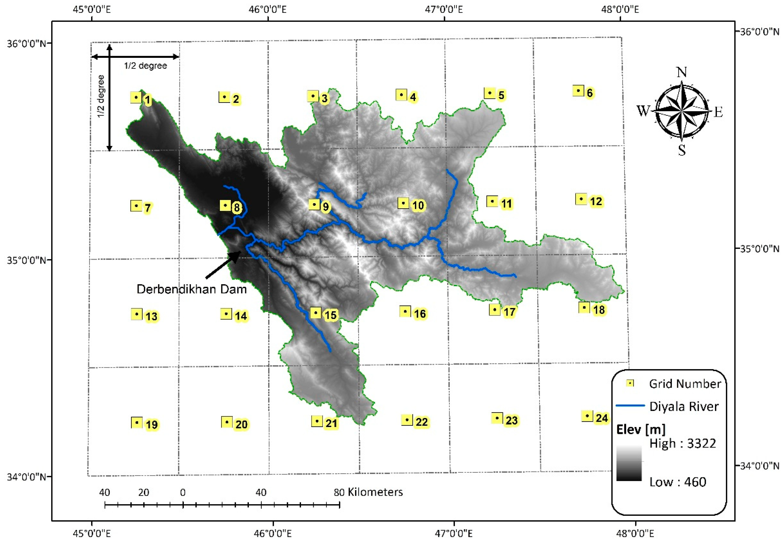
5. Case Study and Data

The developed PR-WG was tested in the Diyala River basin, which is a transboundary basin between Iran and Iraq with a total stream length of 217 km and basin area of 16,760 km² above Derbendikhan Dam, as shown in Figure 3. In previous work, Waheed et al., [5] implemented the daily weather data (e.g., precipitation, maximum and minimum temperature, and wind speed) in this basin at a 0.5° spatial resolution from 1948 to 2006 and explained the implementation procedure. In this follow up study, the historic forcing data were used to validate the proposed PR-WG and test its performance. The reader should refer to the original paper for more details about the data implementation and their validation in the basin.

6. Results and Discussion

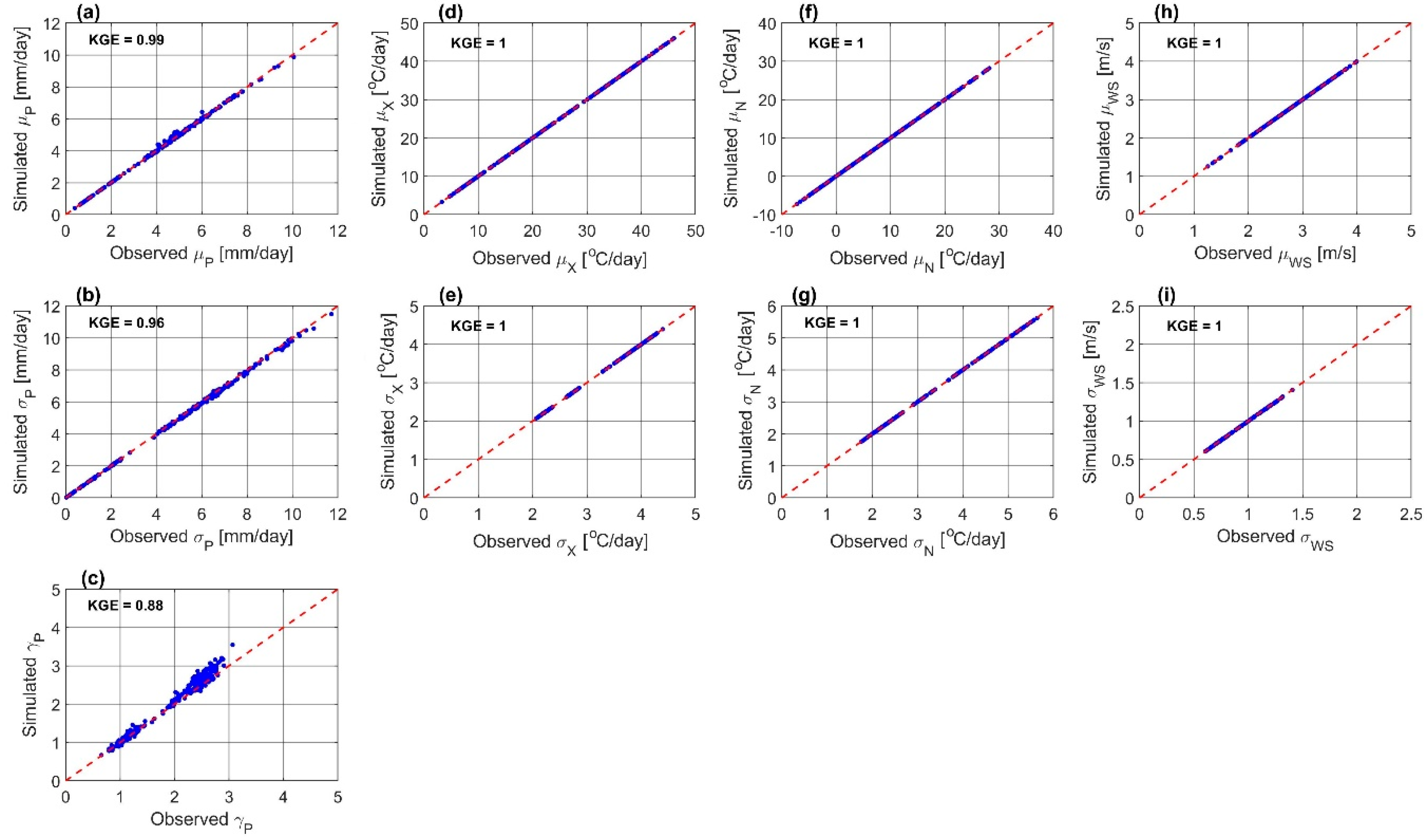
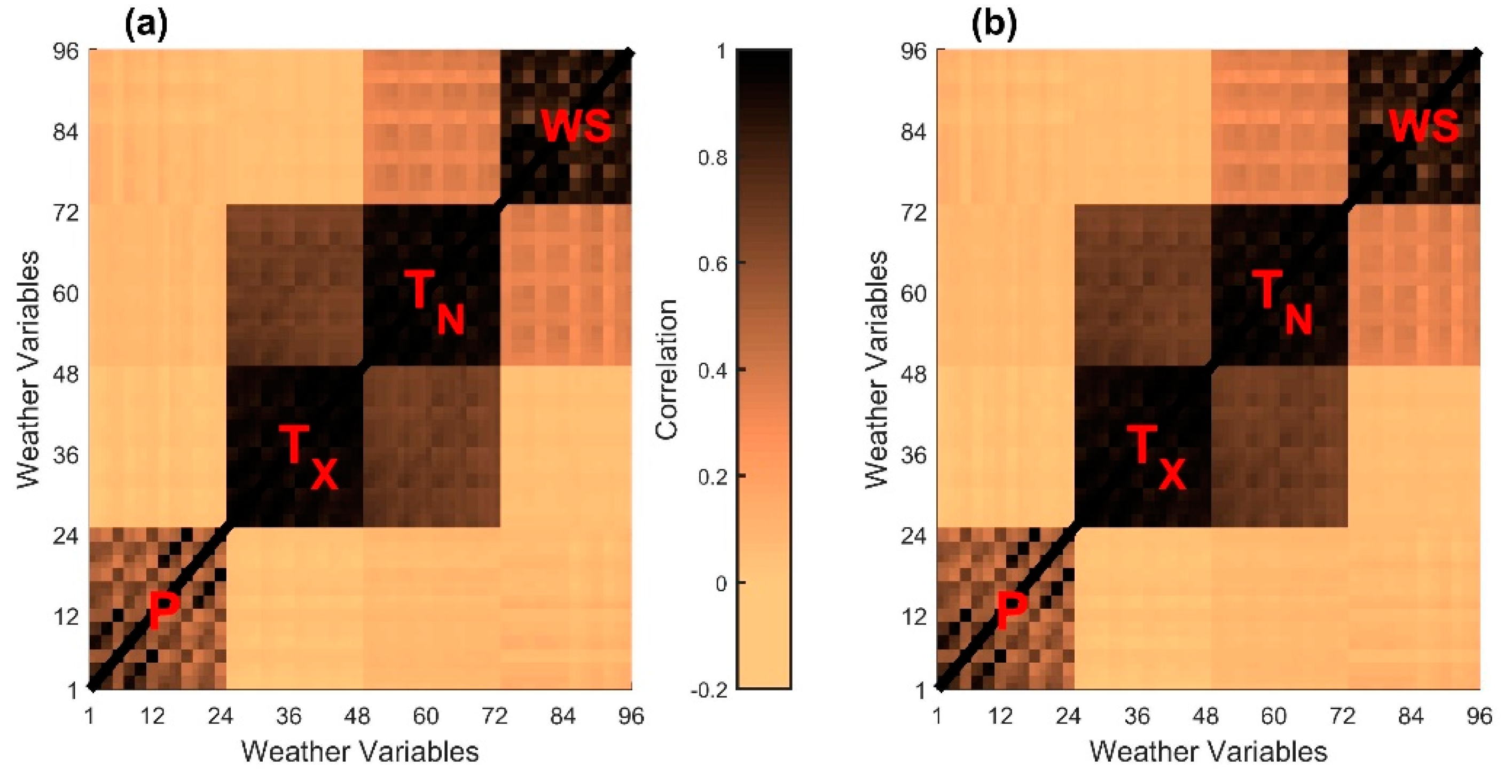
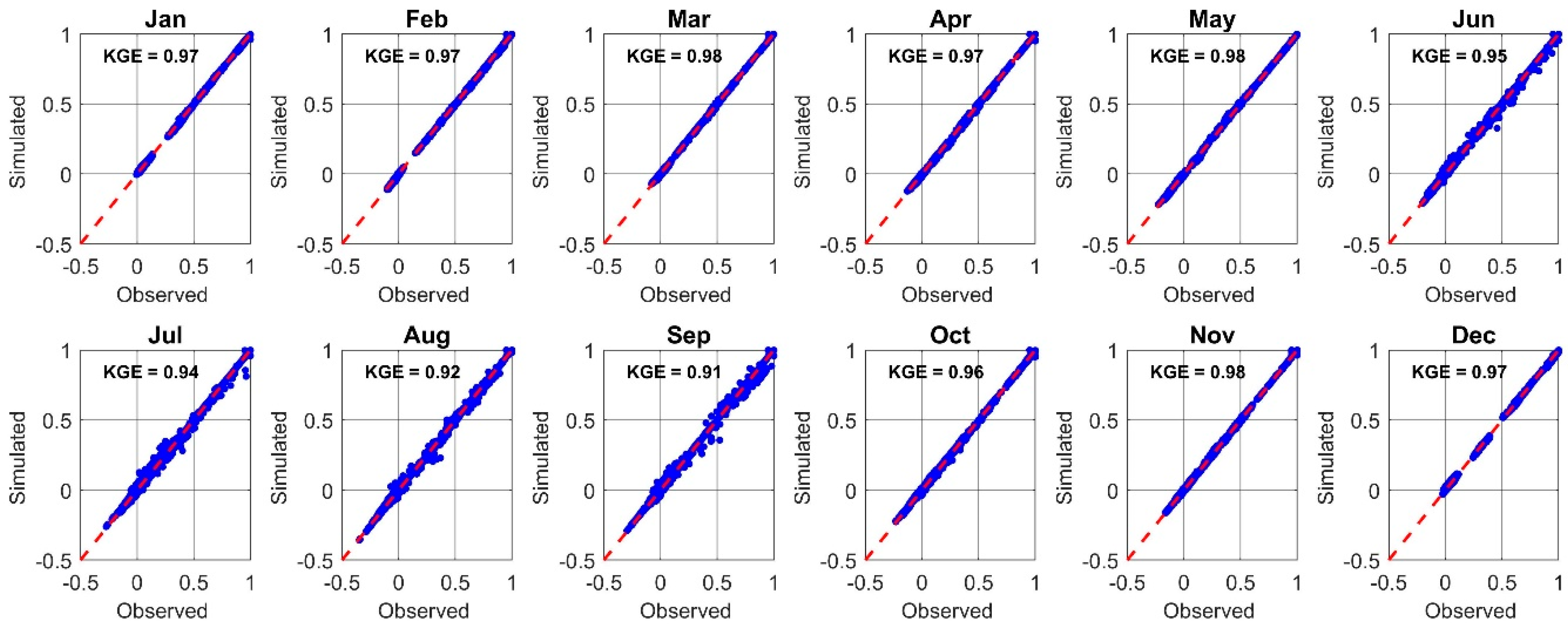
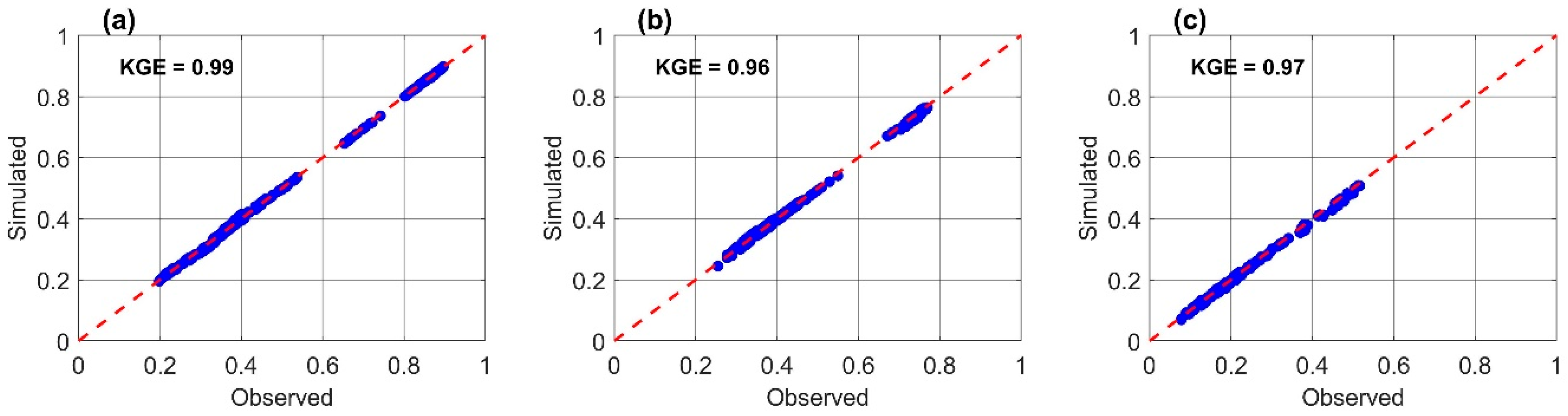
6.1. Model Performance Evaluation

The PR-WG was tested for its daily performance with historic observations for the period between 1948 and 2006, e.g., 58 years, in a grid composed of 24 grid-cells. The Nash–Sutcliffe coefficient efficiency (NSCE; [56]) and the Kling–Gupta efficiency (KGE; [5]) were used to evaluate the PR-WG’s ability to produce spatially correlated precipitation states S similar to the observed values, as follows:

$$\mathrm{NSCE}=1-\frac{{{\displaystyle \sum }}^{}{\left( Si{m}_i-Ob{s}_i \right)}^2}{{{\displaystyle \sum }}^{}{\left( {\mu }_{sim}-Si{m}_i \right)}^2}$$

(17)

$$\mathrm{KGE}=1-\sqrt{{\left(\frac{{\mu }_{sim}}{{\mu }_{obs}}-1\right)}^2+{\left(\frac{{\sigma }_{sim}}{{\sigma }_{obs}}-1\right)}^2+{(\rho -1)}^2}$$

(18)

where Sim and Obs are the simulations (e.g., the PR-WG outcomes) and the observations of the time index t, respectively; µ_obs, σ_obs, µ_sim, and σ_sim are the mean and standard deviation of the observations and simulations (e.g., the PR-WG outcomes), respectively, and ρ is the correlation coefficient between the observations and simulations.

Figure 4 shows the comparison of 10 separate daily simulations each of the same observation length (e.g., 58 years) of PR-WG monthly dry and wet occurrences in gray color dots. The average of these 10 simulations is calculated and plotted in blue dots. The A 1-1 line is also plotted to ease the comparison. It is evident that the model works well to produce the number of dry and wet days, with KGE and NSCE values of 0.97. This result demonstrates the ability of the FTMC to produce the precipitation states well [21,22]. Figure 5 shows a comparison of pairwise correlations of the daily precipitation states calculated for each calendar month. It can be seen that the correlations are captured well by the PR-WG. The overall KGE and NSCE values are 0.98 and 0.99, respectively.

Figure 6 demonstrates the PR-WG performance to produce the statistical parameters (e.g., mean, standard deviation and skewness) of the four weather variables. The comparisons were done on a daily basis at each month for the 24 grid-cells. A daily time step series of 1000 years was generated to reduce the sampling bias and uncertainty in the simulations. However, the daily means of all variables and the standard deviations for T_x, T_N and WS were perfectly produced by the model (KGE ≈1), while σ_p, and γ_p are reasonably preserved (KGE = 0.96 and 0.86; NSCE = 0.98 and 0.93). The slight discrepancies are due to the stochastic nature of the process [57].

Figure 7 shows the daily median values with 0.05 and 0.95 quantiles of the daily values in the bounded areas, and the inverse cumulative distribution function (CDF⁻¹) of the observed and simulated weather variables for grid-cell number 9, which is located in the basin heart (see Figure 3). It is seen that PR-WG well preserves the daily medians for all months. Moreover, the quantile daily estimates show good agreement with the observation quantiles, proving the model’s ability to capture the maximum and minimum daily weather values. It is also noticeable from the inverse CDF the observed and simulated weather values are very close, evincing the validity of the selected distribution types. Furthermore, the simulated daily values of quantile 1 exceed the observation values which demonstrates the model’s ability to produce values beyond the observation ranges.

Figure 8 shows the spatial and cross correlation coefficient matrices of the observations and simulations for one month (e.g., m=1), while Figure 9 shows the spatial and cross correlation comparison for all variables for each m calculated at daily time steps. The number of columns of the V matrix (see Section 4.1) are 4 × 24 = 96. Therefore, the V dimensions are 96 × 96, in which the values are from 1 to 24 for P, 25 to 48 for T_x, 49 to 72 for T_N, and 73 to 96 for the WS. It can be observed from Figure 8 that the observed correlation among the variables varies greatly across them. P and the WS are slightly less spatially correlated as compared with T_x and T_N. These facts are in line with Srivastav and Simonovic [32] and Verdin et al. [15]. It is also noticeable from Figure 8 and Figure 9 that the model preserves the spatial and cross correlation well among the variables. The overall KGE and NSCE values are 0.96 and 0.97, respectively.

Figure 10 demonstrates the PR-WG capability to preserve the Lag-1 day auto-correlations of T_x, T_N and the WS. It is noticeable that the values differ from month to month, they are less for the WS comparing to T_x and T_N. However, the PR-WG captures these monthly variations very well regardless of their magnitudes with the overall KGE and NSCE values of 0.97 and 0.98, respectively.

The results presented here glimpse the model capability to preserve the statistical properties of the observations to synthesize the future scenarios. The proposed model demonstrated the Wilks technique ability to generate anomalies similarly to the observations. It is also seen that the hybrid structure of the AR and Wilks technique leads to generate data that preserve the temporal correlation beside the spatial and cross correlations.

The key advantage of PR-WG is that it is built to be a general model through studying the observation anomalies and mimicking them. Therefore, the model is anticipated to work well in different climate zones and topographies regardless of the data spatial and temporal scale. The model framework is flexible enough for locations observe short-term and long-term variations. Moreover, the user can reduce the cycle data length to meet their scope. e.g., they can use a data window of two weeks (or a week) instead of the monthly window that was used in this study. The computational expensive of implemented the pre-processing stage has to carefully examined.

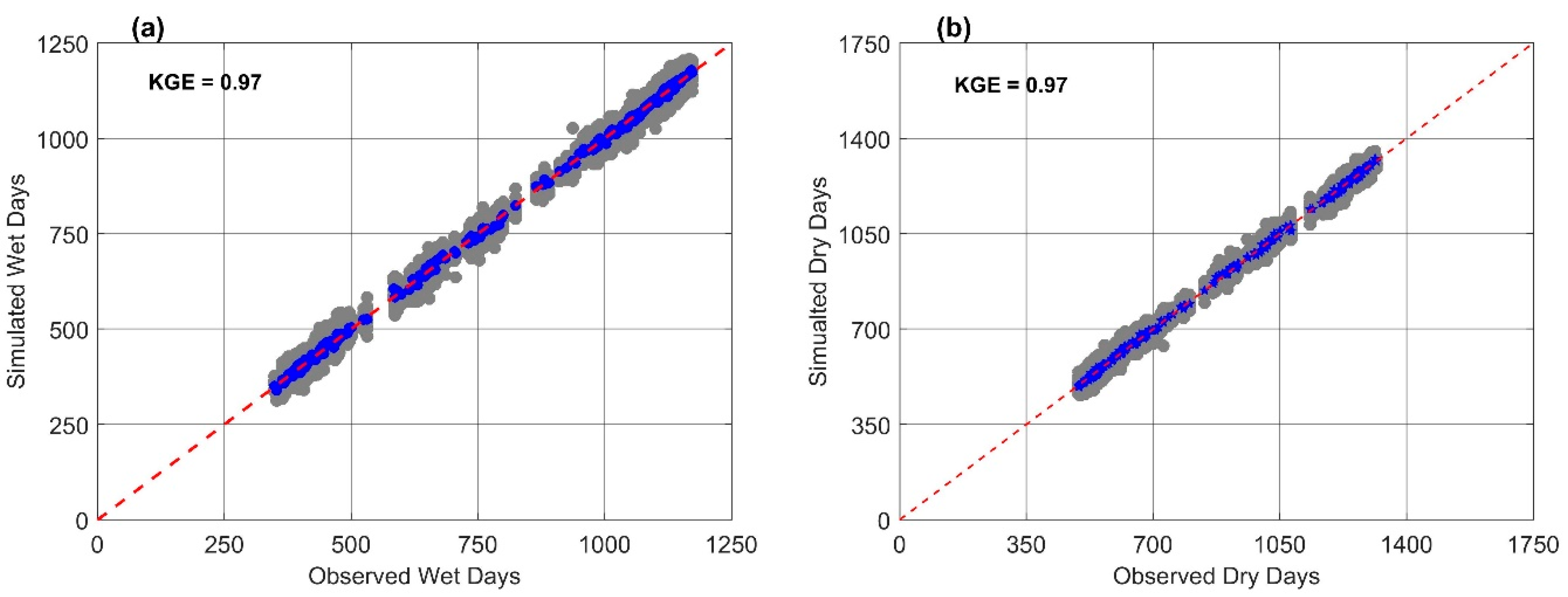
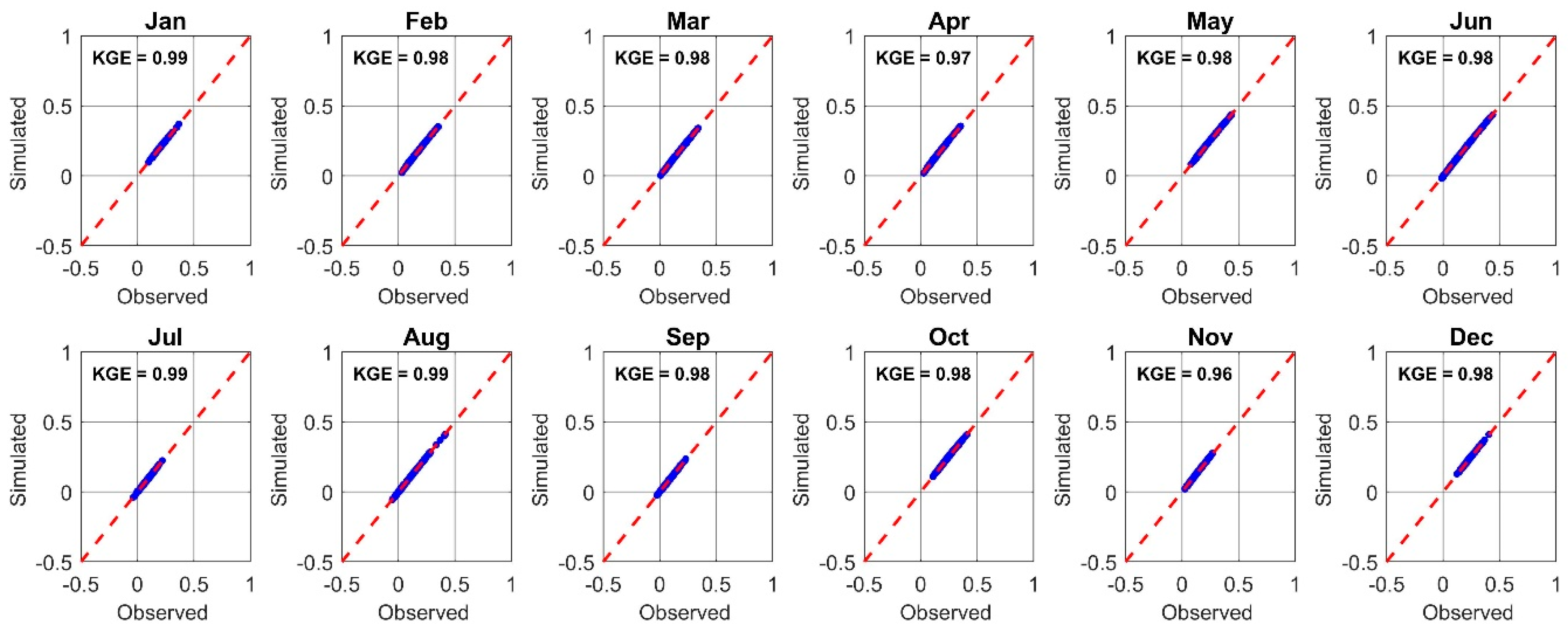
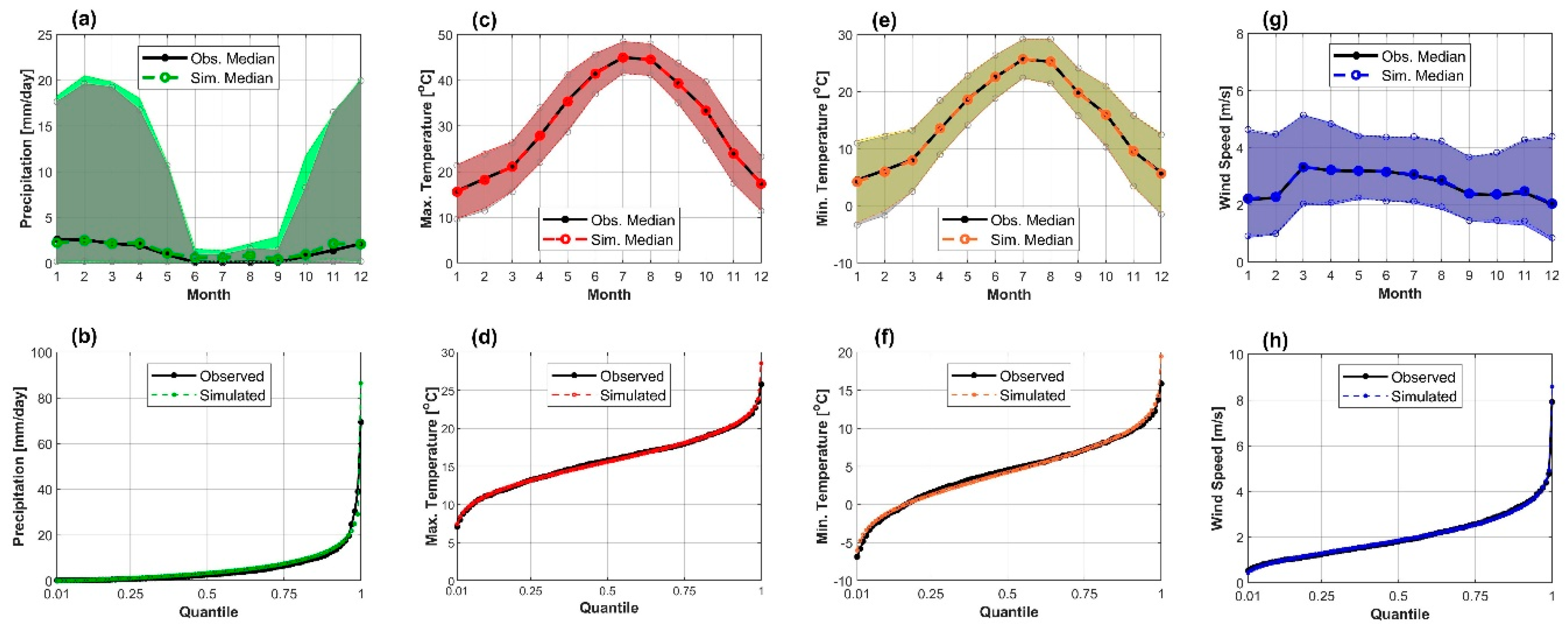
6.2. Model Validation

In some cases, the proposed SWG produces negative daily values for precipitation. [58] indicated that the SN is not suitable when the skewness is greater than 4.5. However, in the study area, values of the skewness have not exceeded 4.5 (see Figure 6c), therefore the SN is applicable. The negatives of the daily values were checked and found to be less than 3% of the whole 1000-year time series in the 24 grid-cells. The suggestion of [32] to round the negative values to zero was considered, but it would affect the number of wet and dry calculations and the statistical parameters of precipitation. Instead, the negatives were rounded to 0.1 mm/day, which is assumed to be the minimum precipitation amount (see Section 3.1). This correction approach for negative values illustrates the slight differences in the simulated σ_p and γ_p (see Figure 5b,c). The user could apply another distribution function in cases where the SN is not applicable such as mixed-exponential [59,60], log-normal, gamma, etc. The key advantage of PR-WG is its flexibility in adopting any distribution of interest, such as these.

The second validation was done by checking if T_N is greater than T_x and was found to be less than 1% of the whole 1000-year time series in the 24 grid-cells. [41] suggested to force T_x to be greater than T_N through setting T_N equal to T_x minus 1. This procedure will affect the auto-correlation of the T_N. Instead, the Chen et al., [57] approach was applied as follows, if T_x ˂ T_N,

$$\begin{gathered} T_{X\left(k,t,m\right)}=T_{N\left(k,t,m\right)}+({\mu }_{\mu x\left(k,m\right)}-{\mu }_{\mu N\left(k,m\right)})+\sqrt{{\sigma }_{X\left(k,m\right)}^2-{\sigma }_{N\left(k,m\right)}^2}\times z_{std\left(k,t,m\right)} \\ for {\mathsf{𝕝}}_{[\sigma X{ }_{\left(k,t,m\right)}\ge \sigma N{ }_{\left(k,t,m\right)}]} \end{gathered}$$

(19)

$$\begin{gathered} T_{X\left(k,t,m\right)}=T_{N\left(k,t,m\right)}+({\mu }_{\mu x\left(k,m\right)}-{\mu }_{\mu N\left(k,m\right)})+\sqrt{{\sigma }_{X\left(k,m\right)}^2-{\sigma }_{N\left(k,m\right)}^2}\times z_{std\left(k,t,m\right)} \\ for {\mathsf{𝕝}}_{[\sigma X{ }_{\left(k,t,m\right)}<\sigma N{ }_{\left(k,t,m\right)}]} \end{gathered}$$

(20)

Equations (19) and (20) are conditioned on the precipitation states. For example, the σ and μ will turn to condition 0 if S = 0. In this case, the T_X is guaranteed to be greater than T_N and the auto, spatial, and cross correlations are preserved since they are multiplied by the anomalies $z_{std}$.

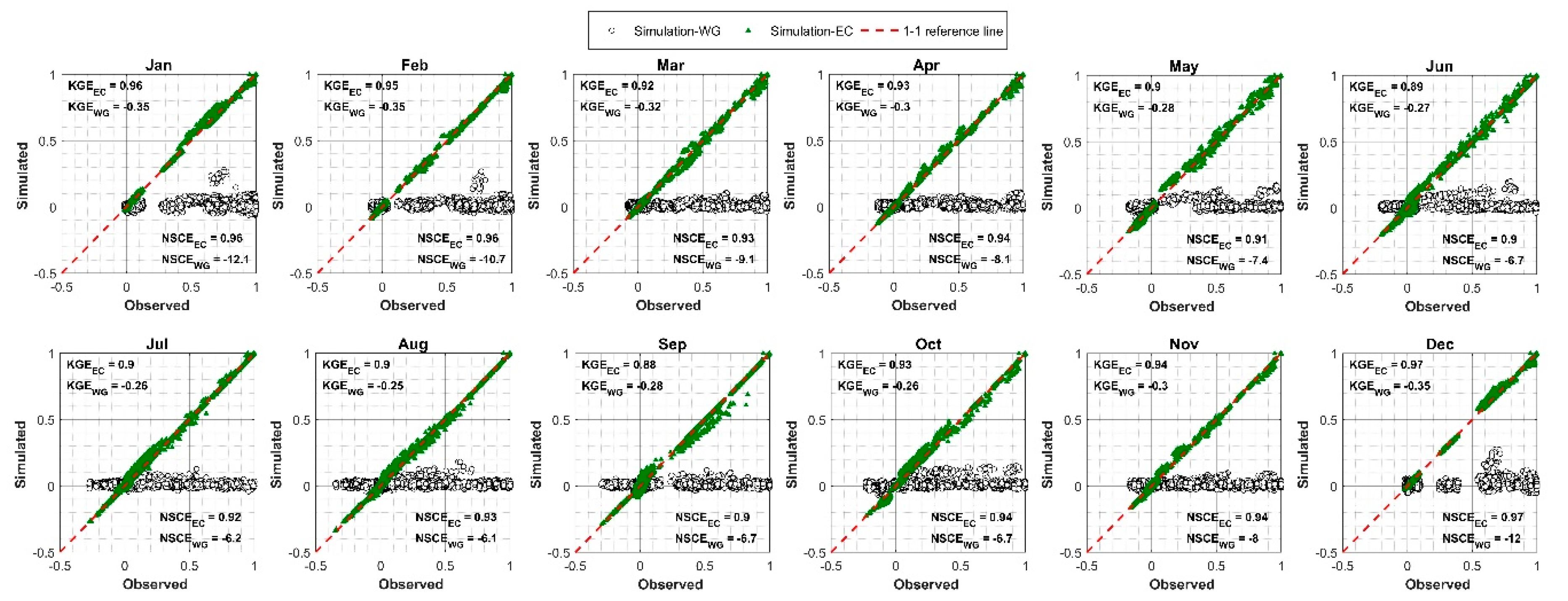
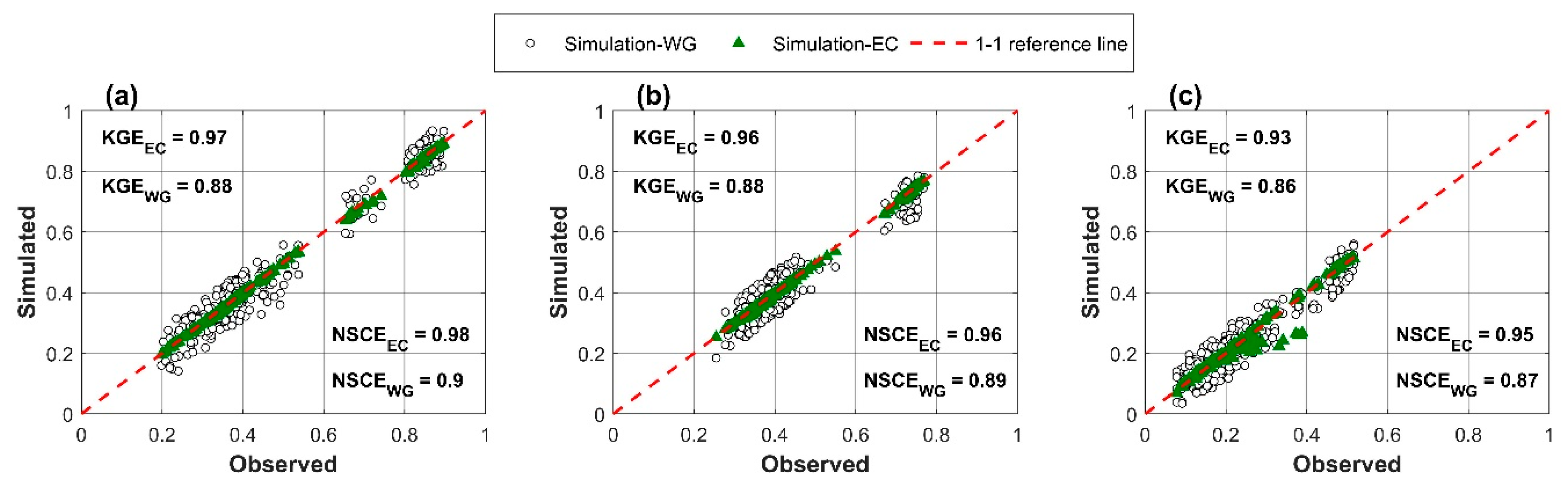
6.3. Model Comparison

For comparison purposes, two SWG models were selected to compare their performances with the PR-WG to further demonstrate the model applicability. The first model is the single site weather generator (WG) developed by Chen et al., [57] and Chen et al., [61]. The second is the two stages weather generator using an empirical copula (EC) approach developed by Li and Babovic [41]. To highlight the unique contribution of the PR-WG model, we focused on the model performances to maintain the spatial, cross, and temporal correlations. Figure 11 shows the daily performances of the WG and EC to for the spatial and cross correlations, while Figure 12 shows the temporal correlations for the sites and month. It is seen that the EC model works well in preserving the spatial, cross, and temporal correlation; the PR-WG is slightly superior to it. However, the KGE and NSCE for the spatial and cross correlations are 0.92 and 0.93, and for the temporal 0.95, and 0.96. It also notable that the WG model poorly preserves the spatial and cross correlations but has good ability to preserve the temporal correlation. This is because the model accounts for the temporal correlation only, where the simulated data were generated independently for all variables and sites which leads to poor spatial and cross correlation accuracy. The KGE and NSCE for the spatial and cross correlations are −0.29 and −8.3, and for the temporal 0.88, and 0.89. Although the EC approach works well in general, the only drawback is that its simulation time period must be identical to the historic observation, which prevents its usage in areas with limited data availability. This is because the post processing stage of the EC model employs a re-ranking technique that extracts the ranked variables directly from the historic observations. Therefore, the model length can only be the same as the historic observations, leading to less flexibility for future scenarios, especially in data scarce regions. The PR-WG has the advantage of producing the simulation length of interest, making it useful in areas with limited data availability besides maintaining the statistical characteristics.

6.4. Simulation of the Future Forecasting Scenarios

The goal of the PR-WG is to be used later for climate variation assessments. The advantage of the model, besides the ability to preserve the statistical characteristics, is its flexibility to alter them to produce a wide range of different scenarios. However, defining the future scenario ranges to test a water resources system’s performance in terms of the climate stress is a difficult task and dependent on many factors, including expert opinions [4].

These future scenarios will be applied in the Diyala River basin to discover the vulnerability of the Derbendikhan Dam and its reservoir. Moreover, different adaptation strategies will be suggested in order to test their capabilities to improve the system performance. Since the model is implemented on a stochastic basis, the future trend insights will be obtained from analyzing the GCM models. Then, this can be fed into the PR-WR to mimic the future trend as well as the statistical properties. For instance, multiplicative factors for the precipitation mean will be applied starting from a 0% change in the historical precipitation and annual linearly increasing (or decreasing) up to the specified value in the final period (e.g., +30% of the historical value). Forms other than the linear change can also be applied to synthesize the future forecast data.

7. Conclusions

It was shown that a PR-WG accurately preserves the statistical properties (mean, standard deviation, and skewness coefficient) of the weather variables (overall KGE and NSCE test values were 0.98). The PR-WG also preserves the spatial, temporal, and cross correlations among the weather variables. While other SWGs may have more features, the one developed in this study enables a bottom-up vulnerability assessment study to be implemented in areas with limited data availability.

The PR-WG effectively estimates the dry and wet day occurrences using a FTMC with overall KGE and NSCE values of 0.97, a result that is in line with those in [21,22]. The results also demonstrate the effectiveness of Wilks’ technique to produce spatially correlated precipitation states (KGE of 0.98; NSCE of 0.99) and spatially and cross correlated weather variables (KGE of 0.96; NSCE of 0.97), as well as temporally correlated variables (KGE of 0.97; NSCE of 0.98). The model is also capable of preserving the maximum and minimum daily weather values as well as producing values beyond the observed ranges. Furthermore, the PR-WG outperforms the EC and WG models in preserving the spatial, cross, and temporal correlations in the meteorological stations.

While the PR-WG was validated in the Diyala River basin, it should be effective and applicable in other places and with other weather variables, such as solar radiation. The advantages of PR-WG are its flexibility to select any distribution function for each weather variable, ability to simulate any number of years within or beyond the historic observation length, capability to generate values outside the observation range, and its ability to produce synthetic scenarios through the alteration of the weather variable parameters for the study of climate change’s impacts. The PR-WG is easy to construct and understand with little computational intensity to build the spatial and cross correlation matrices of the anomalies. Increasing computational power will facilitate the work.

References

1. Hallegatte, S.; Shah, A.; Lempert, R.; Brown, C.; Gill, S. Investment Decision Making under Deep Uncertainty-Application to Climate Change; The World Bank: Washington, DC, USA, 2012. [Google Scholar]
2. Brown, C.; Wilby, R.L. An alternate approach to assessing climate risks. Eos, Trans. Am. Geophys. Union 2012, 93, 401–402. [Google Scholar] [CrossRef]
3. Stephenson, D.; Collins, M.; Rougier, J.C.; Chandler, R.E. Statistical problems in the probabilistic prediction of climate change. Environmetrics 2012, 23, 364–372. [Google Scholar] [CrossRef]
4. Steinschneider, S.; Brown, C. A semiparametric multivariate, multisite weather generator with low-frequency variability for use in climate risk assessments. Water Resour. Res. 2013, 49, 7205–7220. [Google Scholar] [CrossRef]
5. Waheed, S.Q.; Grigg, N.S.; Ramirez, J.A. Variable Infiltration-Capacity Model Sensitivity, Parameter Uncertainty, and Data Augmentation for the Diyala River Basin in Iraq. J. Hydrol. Eng. 2020, 25, 04020040. [Google Scholar] [CrossRef]
6. Culley, S.; Noble, S.; Yates, A.; Timbs, M.; Westra, S.; Maier, H.R.; Giuliani, M.; Castelletti, A. A bottom-up approach to identifying the maximum operational adaptive capacity of water resource systems to a changing climate. Water Resour. Res. 2016, 52, 6751–6768. [Google Scholar] [CrossRef] [Green Version]
7. Weaver, C.P.; Lempert, R.J.; Brown, C.; Hall, J.A.; Revell, D.; Sarewitz, D. Improving the contribution of climate model information to decision making: The value and demands of robust decision frameworks. Wiley Interdiscip. Rev. Clim. Chang. 2012, 4, 39–60. [Google Scholar] [CrossRef]
8. Turner, S.W.; Marlow, D.; Ekström, M.; Rhodes, B.G.; Kularathna, U.; Jeffrey, P. Linking climate projections to performance: A yield-based decision scaling assessment of a large urban water resources system. Water Resour. Res. 2014, 50, 3553–3567. [Google Scholar] [CrossRef]
9. Steinschneider, S.; Wi, S.; Brown, C. The integrated effects of climate and hydrologic uncertainty on future flood risk assessments. Hydrol. Process. 2014, 29, 2823–2839. [Google Scholar] [CrossRef]
10. Zhang, E.; Yin, X.; Xu, Z.; Yang, Z. Bottom-up quantification of inter-basin water transfer vulnerability to climate change. Ecol. Indic. 2018, 92, 195–206. [Google Scholar] [CrossRef]
11. Whateley, S.; Steinschneider, S.; Brown, C. A climate change range-based method for estimating robustness for water resources supply. Water Resour. Res. 2014, 50, 8944–8961. [Google Scholar] [CrossRef]
12. Moody, P.; Brown, C. Robustness indicators for evaluation under climate change: Application to the upper Great Lakes. Water Resour. Res. 2013, 49, 3576–3588. [Google Scholar] [CrossRef]
13. Steinschneider, S.; McCrary, R.; Wi, S.; Mulligan, K.B.; Mearns, L.O.; Brown, C. Expanded Decision-Scaling Framework to Select Robust Long-Term Water-System Plans under Hydroclimatic Uncertainties. J. Water Resour. Plan. Manag. 2015, 141, 04015023. [Google Scholar] [CrossRef]
14. Wilks, D. Multisite generalization of a daily stochastic precipitation generation model. J. Hydrol. 1998, 210, 178–191. [Google Scholar] [CrossRef]
15. Verdin, A.P.; Rajagopalan, B.; Kleiber, W.; Podestá, G.; Bert, F. BayGEN: A Bayesian Space-Time Stochastic Weather Generator. Water Resour. Res. 2019, 55, 2900–2915. [Google Scholar] [CrossRef]
16. Wilks, D.S. A gridded multisite weather generator and synchronization to observed weather data. Water Resour. Res. 2009, 45. [Google Scholar] [CrossRef] [Green Version]
17. Wilks, D.S. Statistical Methods in the Atmospheric Sciences; Academic Press: Cambridge, MA, USA, 2011. [Google Scholar]
18. Furrer, E.; Katz, R.W. Improving the simulation of extreme precipitation events by stochastic weather generators. Water Resour. Res. 2008, 44. [Google Scholar] [CrossRef]
19. Jie, C.; Brissette, F.P.; Zhang, X.J. A multi-site stochastic weather generator for daily precipitation and temperature. Trans. ASABE 2014, 57, 1375–1391. [Google Scholar]
20. Chen, J.; Brissette, F.P. Stochastic generation of daily precipitation amounts: Review and evaluation of different models. Clim. Res. 2014, 59, 189–206. [Google Scholar] [CrossRef] [Green Version]
21. Chen, J.; Brissette, F.P. Comparison of five stochastic weather generators in simulating daily precipitation and temperature for the Loess Plateau of China. Int. J. Climatol. 2014, 34, 3089–3105. [Google Scholar] [CrossRef]
22. Acharya, N.; Frei, A.; Chen, J.; DeCristofaro, L.; Owens, E.M. Evaluating Stochastic Precipitation Generators for Climate Change Impact Studies of New York City’s Primary Water Supply. J. Hydrometeorol. 2017, 18, 879–896. [Google Scholar] [CrossRef]
23. Mukundan, R.; Acharya, N.; Gelda, R.K.; Frei, A.; Owens, E.M. Modeling streamflow sensitivity to climate change in New York City water supply streams using a stochastic weather generator. J. Hydrol. Reg. Stud. 2019, 21, 147–158. [Google Scholar] [CrossRef]
24. Mehrotra, R.; Westra, S.; Sharma, A.; Srikanthan, R. Continuous rainfall simulation: 2. A regionalized daily rainfall generation approach. Water Resour. Res. 2012, 48, 48. [Google Scholar] [CrossRef] [Green Version]
25. Richardson, C.W. Stochastic simulation of daily precipitation, temperature, and solar radiation. Water Resour. Res. 1981, 17, 182–190. [Google Scholar] [CrossRef]
26. Qian, B.; Xu, H. Multisite stochastic weather models for impact studies. Int. J. Clim. 2002, 22, 1377–1397. [Google Scholar] [CrossRef]
27. Brissette, F.; Khalili, M.; Leconte, R. Efficient stochastic generation of multi-site synthetic precipitation data. J. Hydrol. 2007, 345, 121–133. [Google Scholar] [CrossRef]
28. Srikanthan, R.; Pegram, G. A nested multisite daily rainfall stochastic generation model. J. Hydrol. 2009, 371, 142–153. [Google Scholar] [CrossRef]
29. Baigorria, G.A.; Jones, J.W. GiST: A Stochastic Model for Generating Spatially and Temporally Correlated Daily Rainfall Data. J. Clim. 2010, 23, 5990–6008. [Google Scholar] [CrossRef]
30. Leander, R.; Buishand, T.A. A daily weather generator based on a two-stage resampling algorithm. J. Hydrol. 2009, 374, 185–195. [Google Scholar] [CrossRef]
31. King, L.M.; McLeod, A.I.; Simonovic, S.P. Improved Weather Generator Algorithm for Multisite Simulation of Precipitation and Temperature. JAWRA J. Am. Water Resour. Assoc. 2015, 51, 1305–1320. [Google Scholar] [CrossRef] [Green Version]
32. Srivastav, R.K.; Simonovic, S.P. Multi-site, multivariate weather generator using maximum entropy bootstrap. Clim. Dyn. 2014, 44, 3431–3448. [Google Scholar] [CrossRef]
33. Khalili, M.; Brissette, F.; Leconte, R. Effectiveness of Multi-Site Weather Generator for Hydrological Modeling1. JAWRA J. Am. Water Resour. Assoc. 2011, 47, 303–314. [Google Scholar] [CrossRef]
34. Murray, V.; Ebi, K.L. IPCC Special Report on Managing the Risks of Extreme Events and Disasters to Advance Climate Change Adaptation (SREX). J. Epidemiol. Community Heal. 2012, 66, 759–760. [Google Scholar] [CrossRef] [PubMed]
35. Mehrotra, R.; Li, J.; Westra, S.; Sharma, A. A programming tool to generate multi-site daily rainfall using a two-stage semi parametric model. Environ. Model. Softw. 2015, 63, 230–239. [Google Scholar] [CrossRef]
36. Wang, W.; Flanagan, D.C.; Yin, S.; Yu, B. Assessment of CLIGEN precipitation and storm pattern generation in China. Catena 2018, 169, 96–106. [Google Scholar] [CrossRef]
37. John, S.; Pailleux, J.; Thielen, J.; Arritt, R.; Hamill, T.; Luo, L.; Martin, E.; McCollor, D.; Pappenberger, F. Summary of recommendations of the first workshop on Postprocessing and Downscaling Atmospheric Forecasts for Hydrologic Applications held at Météo-France, Toulouse, France, 15–18 June 2009. Atmos. Sci. Lett. 2010, 11, 59–63. [Google Scholar]
38. Li, Z. A new framework for multi-site weather generator: A two-stage model combining a parametric method with a distribution-free shuffle procedure. Clim. Dyn. 2013, 43, 657–669. [Google Scholar] [CrossRef]
39. Li, C.; Sinha, E.; Horton, D.E.; Diffenbaugh, N.S.; Michalak, A.M. Joint bias correction of temperature and precipitation in climate model simulations. J. Geophys. Res. Atmos. 2014, 119, 13–153. [Google Scholar] [CrossRef]
40. Chen, J.; Li, C.; Brissette, F.P.; Chen, H.; Wang, M.; Essou, G.R. Impacts of correcting the inter-variable correlation of climate model outputs on hydrological modeling. J. Hydrol. 2018, 560, 326–341. [Google Scholar] [CrossRef]
41. Li, X.; Babovic, V. A new scheme for multivariate, multisite weather generator with inter-variable, inter-site dependence and inter-annual variability based on empirical copula approach. Clim. Dyn. 2018, 52, 2247–2267. [Google Scholar] [CrossRef]
42. Guillermo, A.B.; Jones, J.W. GiST: A stochastic model for generating spatially and temporally correlated daily Investment Decision Making under Deep Uncertainty—Application to Climate Change rainfall data. What kind of data is needed to identify climate impacts? How can data be managed and organized through data catalogues? J. Clim. 2010, 23, 5990–6008. [Google Scholar]
43. Haugen, A.; Bertolin, C.; Leijonhufvud, G.; Olstad, T.; Broström, T. A Methodology for Long-Term Monitoring of Climate Change Impacts on Historic Buildings. Geosciences 2018, 8, 370. [Google Scholar] [CrossRef] [Green Version]
44. Li, Z.; Brissette, F.; Chen, J. Assessing the applicability of six precipitation probability distribution models on the Loess Plateau of China. Int. J. Clim. 2013, 34, 462–471. [Google Scholar] [CrossRef]
45. Mehan, S.; Guo, T.; Gitau, M.W.; Flanagan, D.C. Comparative Study of Different Stochastic Weather Generators for Long-Term Climate Data Simulation. Climate 2017, 5, 26. [Google Scholar] [CrossRef]
46. Nicks, A.D.; Gander, G.A. CLIGEN: A Weather Generator for Climate Inputs to Water Resource and Other Models. In Proceedings of the Fifth International Conference on Computers in Agriculture, Orlando, FL, USA, 6–9 February 1994; Available online: https://www.worldcat.org/title/cligen-a-weather-generator-for-climate-inputs-to-water-resource-and-other-models/oclc/693437629 (accessed on 7 August 2020).
47. Harmel, R.D.; Richardson, C.W.; Hanson, C.L.; Johnson, G.L. Evaluating the Adequacy of Simulating Maximum and Minimum Daily Air Temperature with the Normal Distribution. J. Appl. Meteorol. 2002, 41, 744–753. [Google Scholar] [CrossRef]
48. Harmel, R.D.; Richardson, C.W.; Hanson, C.L.; Johnson, G.L. Simulating maximum and minimum daily temperature with the normal distribution. In Proceedings of the 2001 ASAE Annual Meeting. American Society of Agricultural and Biological Engineers, Sacramento, CA, USA, 29 July–1 August 2001. [Google Scholar]
49. Pobočíková, I.; Sedliačková, Z.; Michalková, M. Application of Four Probability Distributions for Wind Speed Modeling. Procedia Eng. 2017, 192, 713–718. [Google Scholar] [CrossRef]
50. Back, L.E.; Bretherton, C.S. The Relationship between Wind Speed and Precipitation in the Pacific ITCZ. J. Clim. 2005, 18, 4317–4328. [Google Scholar] [CrossRef]
51. Saralees, N. A review of results on sums of random variables. Acta Appl. Math. 2008, 103, 131–140. [Google Scholar]
52. Mehrotra, R.; Srikanthan, R.; Sharma, A. A comparison of three stochastic multi-site precipitation occurrence generators. J. Hydrol. 2006, 331, 280–292. [Google Scholar] [CrossRef]
53. Khalili, M.; Leconte, R.; Brissette, F. Stochastic Multisite Generation of Daily Precipitation Data Using Spatial Autocorrelation. J. Hydrometeorol. 2007, 8, 396–412. [Google Scholar] [CrossRef]
54. Chen, J.; Brissette, F.P.; Zhang, X. Hydrological Modeling Using a Multisite Stochastic Weather Generator. J. Hydrol. Eng. 2016, 21, 04015060. [Google Scholar] [CrossRef]
55. Maree, S.C. Correcting Non Positive Definite Correlation Matrices. Bachelor’s Thesis, Department of Applied Mathematics, Delft University of Technology, Delft, Australia, 2012. [Google Scholar]
56. Eamonn, N.J.; Sutcliffe, J.V. River flow forecasting through conceptual models part I—A discussion of principles. J. Hydrol. 1970, 10, 282–290. [Google Scholar]
57. Chen, J.; Brissette, F.P.; Leconte, R.; Caron, A. A Versatile Weather Generator for Daily Precipitation and Temperature. Trans. ASABE 2012, 55, 895–906. [Google Scholar] [CrossRef]
58. Meyer, C. General Description of the CLIGEN Model and Its History; USDA-ARS National Soil Erosion Laboratory: West Lafayette, IN, USA, 2011. [Google Scholar]
59. Rolda´n, J.; Woolhiser, D.A.; Roldán, J. Stochastic daily precipitation models: 1. A comparison of occurrence processes. Water Resour. Res. 1982, 18, 1451–1459. [Google Scholar] [CrossRef]
60. Wilks, D.S. Simultaneous stochastic simulation of daily precipitation, temperature and solar radiation at multiple sites in complex terrain. Agric. For. Meteorol. 1999, 96, 85–101. [Google Scholar] [CrossRef]
61. Chen, J.; Brissette, F.; Leconte, R. A daily stochastic weather generator for preserving low-frequency of climate variability. J. Hydrol. 2010, 388, 480–490. [Google Scholar] [CrossRef]
Figure 1. Schematic flowchart of the daily weather generation processes.
Climate 08 00093 g001
Figure 2. (a) An example of Wilks’ technique for precipitation states; (b) and (c) are examples of Wilks’ technique to obtain φz for Tx and WS, respectively, for station k of month m.
Climate 08 00093 g002
Figure 3. Diyala River basin in Iraq with grid-cell numbers.
Climate 08 00093 g003
Figure 4. Comparison of the daily precipitation states between the observations and simulations for all months and grid-cells.
Climate 08 00093 g004
Figure 5. Comparison of the daily precipitation state correlation between the observations and simulations for each month for all grid-cells.
Climate 08 00093 g005
Figure 6. Comparisons of the daily statistic parameters of the observations and simulations. (ac) are the mean, standard deviation, and skewness of P. (dg) are the mean and standard deviation of Tx and TN. (h,i) are the mean and standard deviation of the WS.
Climate 08 00093 g006
Figure 7. Comparisons of the daily observed and simulated values for the medians with daily 0.05 and 0.95 quantiles in the bounded areas, and the CDF−1 for the four weather variables.
Climate 08 00093 g007
Figure 8. Spatial and cross correlation coefficients of the daily observed (a) and simulated variables (b).
Climate 08 00093 g008
Figure 9. Spatial and cross correlation comparison of the daily weather variables for each month.
Climate 08 00093 g009
Figure 10. Lag-1 day auto-correlations of the weather variables Tx, TN, and WS, respectively, for all months.
Climate 08 00093 g010
Figure 11. Performance evaluation for empirical copula (EC) and weather generator (WG) models for preserving the spatial and cross correlations of the weather variables for each month.
Climate 08 00093 g011
Figure 12. Monthly performance evaluation for EC and WG models for preserving the temporal correlation (Lag-1 day) of the weather variables.
Climate 08 00093 g012