Kelvin/Rossby Wave Partition of Madden-Julian Oscillation Circulations

Department of Earth and Planetary Sciences, Yale University, New Haven, CT 06511, USA
Climate 2021, 9(1), 2; https://0-doi-org.brum.beds.ac.uk/10.3390/cli9010002
Submission received: 16 November 2020
/
Revised: 13 December 2020
/
Accepted: 16 December 2020
/
Published: 25 December 2020
(This article belongs to the Special Issue Climate Change Dynamics and Modeling: Future Perspectives)
Abstract
:The Madden Julian Oscillation (MJO) is a large-scale convective and circulation system that propagates slowly eastward over the equatorial Indian and Western Pacific Oceans. Multiple, conflicting theories describe its growth and propagation, most involving equatorial Kelvin and/or Rossby waves. This study partitions MJO circulations into Kelvin and Rossby wave components for three sets of data: (1) a modeled linear response to an MJO-like heating; (2) a composite MJO based on atmospheric sounding data; and (3) a composite MJO based on data from a Lagrangian atmospheric model. The first dataset has a simple dynamical interpretation, the second provides a realistic view of MJO circulations, and the third occurs in a laboratory supporting controlled experiments. In all three of the datasets, the propagation of Kelvin waves is similar, suggesting that the dynamics of Kelvin wave circulations in the MJO can be captured by a system of equations linearized about a basic state of rest. In contrast, the Rossby wave component of the observed MJO’s circulation differs substantially from that in our linear model, with Rossby gyres moving eastward along with the heating and migrating poleward relative to their linear counterparts. These results support the use of a system of equations linearized about a basic state of rest for the Kelvin wave component of MJO circulation, but they question its use for the Rossby wave component.
1. Introduction
The Madden Julian Oscillation (MJO) is a large-scale tropical convective and circulation system that moves slowly eastward over the warm equatorial waters of the Indian and Western Pacific Oceans [1,2,3]. Its large-scale envelope of enhanced moist convection comprises smaller scale convective systems that propagate both eastward and westward [4,5,6]. Its heaviest rainfall is accompanied by a deep moisture anomaly, and trailed by strong low-level westerly wind perturbations [7]. Not only does the MJO cause strong variations in winds and precipitation in the equatorial region [8], but it also modulates the frequency and intensity of tropical cyclones in the Atlantic, Indian, and Pacific Oceans [9,10], as well as the timing and intensity of Asian and North American monsoons [11,12,13].
Over the years, dozens of different theories have been proposed to explain the growth and propagation of the MJO, mentioning many different physical processes, such as enhanced surface evaporation due to the MJO’s perturbation winds [14,15], frictional convergence to the east of the MJO’s convective center [16,17], radiation [18], baroclinic instability [19], and upscale transports by smaller disturbances [20]. The question of which of these processes are the most important has not been resolved with time, with one very recent study noting the fundamentally different nature of 4 current MJO theories [21], a list which is by no means exhaustive. Moreover, while there has been some improvement in MJO representations in climate models, many still produce MJO’s that are too weak, lack eastward propagation, and/or have the wrong period [22,23,24].
In this study, we consider the question of how the horizontal circulation of the MJO is partitioned between two wave types: the Kelvin wave and the Rossby wave. We examine three sets of data relevant to MJO circulation: (1) a modeled linear response to an MJO-like heating; (2) a composite MJO based on atmospheric sounding data [25]; and (3) a composite MJO simulated with a Lagrangian Atmospheric Model (LAM) [26]. In each case, we project the total circulation onto a theoretical atmospheric Kelvin wave, and we consider both the Kelvin wave component of the circulation and the residual circulation when the Kelvin wave is removed, which generally resembles a Rossby wave. We do this for each of three stages of the MJO’s convective life cycle: developing, mature, and dissipating [25]. This study is in the spirit of two previous papers written by the author, one in which the structure of the two-day wave was systemically decomposed and compared to linear theory [27], and another in which the vertical structure of the MJO was broken down into modal components [28].
2. Materials and Methods
2.1. Linear Model
In order to illustrate the fundamental dynamics MJO circulations, we make use of the linear model developed by Haertel and Kiladis [27] and modified by Haertel et al. [28]. It simulates atmospheric responses to prescribed heatings and coolings on a beta-plane using the primitive equations linearized about a basic state of rest [29]. This system of equations is the basis for most modern theories of the MJO [21]. In order to simplify solutions, and, in particular, to make them identical to those of shallow water equations on a beta-plane [30], for most simulations, we use a heating with a vertical structure for that of the first vertical mode and include a rigid upper boundary near the top of the troposphere [27,28,29]. We show below that this simple system captures most of the gross horizontal and vertical structure of the MJO, and, in particular, is useful for illustrating how MJO circulations are partitioned between Kelvin and Rossby waves. Towards this end, we project simulated 850–200 hPa wind shear and mean tropospheric temperature onto Kelvin wave structure using the algorithm described in Appendix A.
2.2. Sounding Observations and Compositing Method
After simulating linear responses to idealized heatings to illustrate some basic equatorial dynamics relevant to MJO circulations, we then partition the observed horizontal structure of the MJO into components associated with Kelvin and Rossby waves. We use the composite MJO structure created by Reference [25] for this purpose. It was constructed by tracking 44 observed MJOs for the period 1996 to 2009 and analyzing atmospheric sounding data for initiating, mature, and dissipating stages of the MJO’s convective envelope. This composite is unique in that it uses a coordinate system centered on the MJO’s convection, and it incorporates no model forecast data (i.e., is a purely observational composite as opposed to those based on model reanalyses). The observed composite MJO includes data from all seasons. For more complete details on the compositing method, the reader is referred to Reference [25].
2.3. Lagrangian Atmospheric Model
We also apply the Kelvin/Rossby partitioning technique to MJO’s simulated with our Lagrangian Atmospheric Model (LAM) [26,31,32]. The LAM predicts motions of individual air parcels using Newtonian mechanics, and uses a unique convective parameterize to redistribute parcels vertically in regions with convective instability. In numerous previous studies, it has been shown to simulate robust and realistic MJOs [25,26,32,33,34,35]. The equivalent Eulerian resolution of the model is roughly 3.75/1.875 degrees longitude/latitude, with a 29 hPa vertical spacing. Nineteen MJOs are composited for a 4-year simulation forced with climatological monthly average sea surface temperatures (SSTs) for the years 1998–2009.
3. Results
3.1. Linear Atmospheric Responses to Stationary Heating
3.1.1. Dry Waves
As a prelude to decomposing the MJO’s circulation into Kelvin and Rossby wave components, we begin by illustrating some relevant equatorial dynamics with our linear model. Consider a transient equatorial heating of the following form:
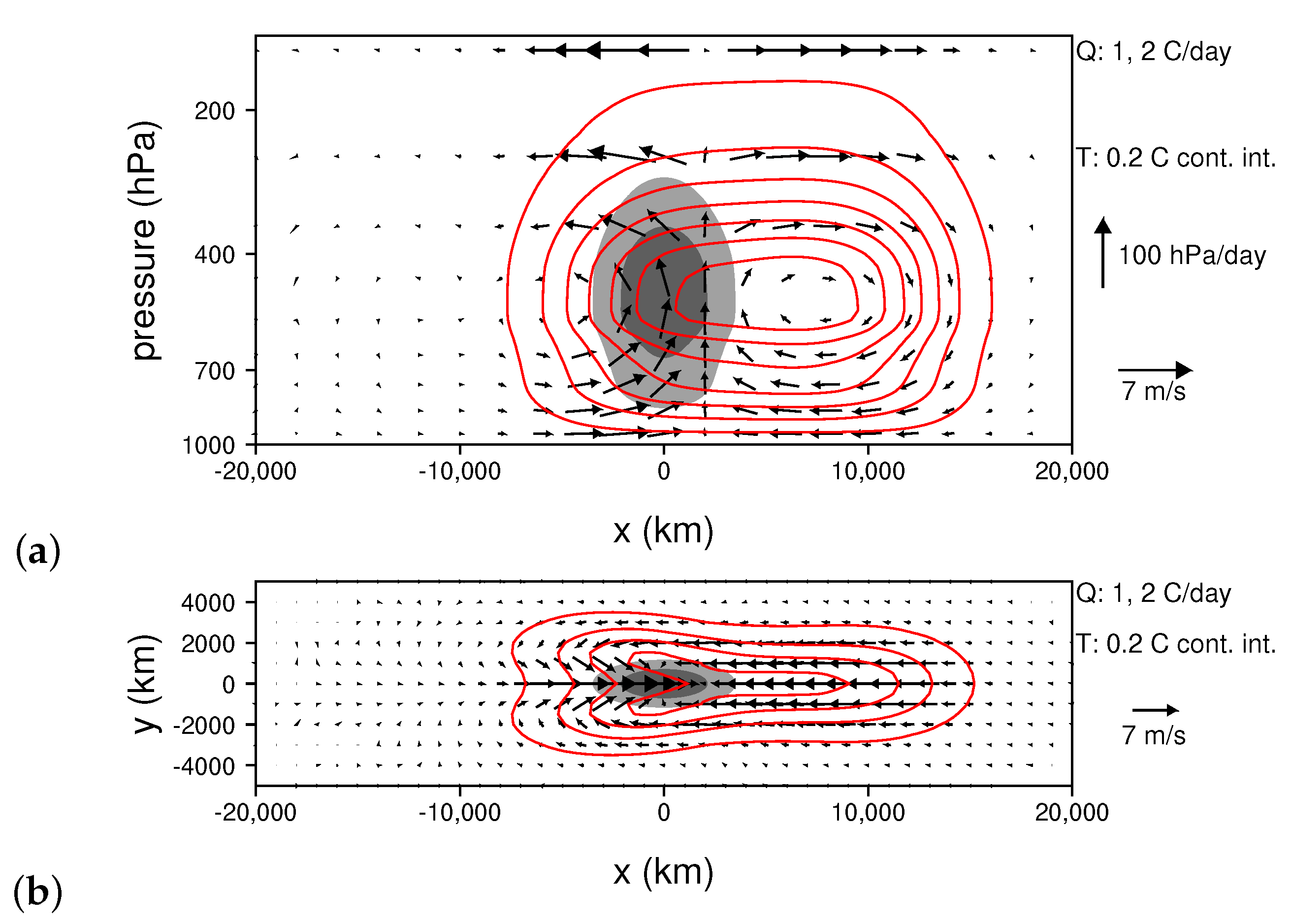
where is the vertical structure of heating for the first vertical mode (e.g., Reference [27]), rx = 3330 km, ry = 1110 km, x is displacement in the east-west direction, y is displacement in the north-south direction, , and p is pressure. We apply this heating for three days and plot atmospheric circulations at 3 and 5 days in Figure 1. The heating generates a warm anomaly with the same vertical structure that spreads slowly westward and more rapidly to the east, with low-level zonal wind convergence and upper-level zonal wind divergence centered just east of the heating (Figure 1a). A birds-eye view of the atmospheric response to the heating reveals positive tropospheric temperature anomalies co-located with low-level easterlies to the east of the heating, which is the signature of an equatorial Kelvin wave, and cyclonic gyres forming to the west of the heating indicative of an equatorial Rossby wave (Figure 1b [30]). Note that, for our linear model, contours of average tropospheric temperature have the same pattern as those of upper-level geopotential; we plot temperature anomalies because they do not depend on a lower-boundary condition, and this leads to a more straightforward comparison with observations. After the heating is turned off, the waves separate so that their individual structures may be more clearly seen (Figure 1c,d), with the Kelvin wave propagating more rapidly than the Rossby wave. The maintenance of uniform vertical structures throughout this simulation (Figure 1a,c) is a consequence of using the theoretical structure for the first vertical mode to construct the heating (Equation (1)) and including a rigid lid above the heating, so that only the first vertical mode is excited. As we discuss in more detail below, including the rigid lid greatly simplifies the dynamics and theoretical interpretation of the simulation and, owing to the large horizontal scale of the MJO, does not drastically alter the horizontal structure of the atmospheric response.
3.1.2. Moist Waves
Next, we consider, a second experiment, in which we make two small modifications to the linear model: (1) we assume that 70 percent of the adiabatic temperature change due to vertical motion is canceled by changes in convective heating; and (2) we reduce the maximum in the amplitude of the prescribed heating by a factor of three to 1 C/day. The first change essentially converts dry waves to “moist” waves and has a number of justifications. First, in the deep tropics over warm oceans where the MJO occurs, the atmosphere’s basic state is one that includes moist convection modulated by large-scale waves. Convection is enhanced where there is large-scale upward motion, and it is reduced where there is large-scale downward motion. It can also be anticipated based on a moisture or moist static energy budget; regions with deep upward motion have low-level convergence convergence of moisture and/or high moist static energy air, and regions with deep downward motion have low-level divergence of moisture and/or high most static energy air. Third, there is empirical evidence that tropical waves have a substantially lower equivalent depth than is predicted by dry dynamics [8] and that this reduction in equivalent depth is indeed a result of partial canceling of adiabatic temperature due to vertical motion by convective heating [27,28]. Here, we use a 70 percent cancellation for illustrative purposes, as it reduces the Kelvin wave speed by roughly a factor of two; below, we increase this to 85 percent, which yields an equivalent depth for moist waves that is consistent with that of observed convectively coupled waves [8]. The reason we reduce the amplitude of the prescribed heating is that it now represents only a portion of the total convective heating, and we want the amplitude of the total heating to be consistent with that observed in the MJO [7].
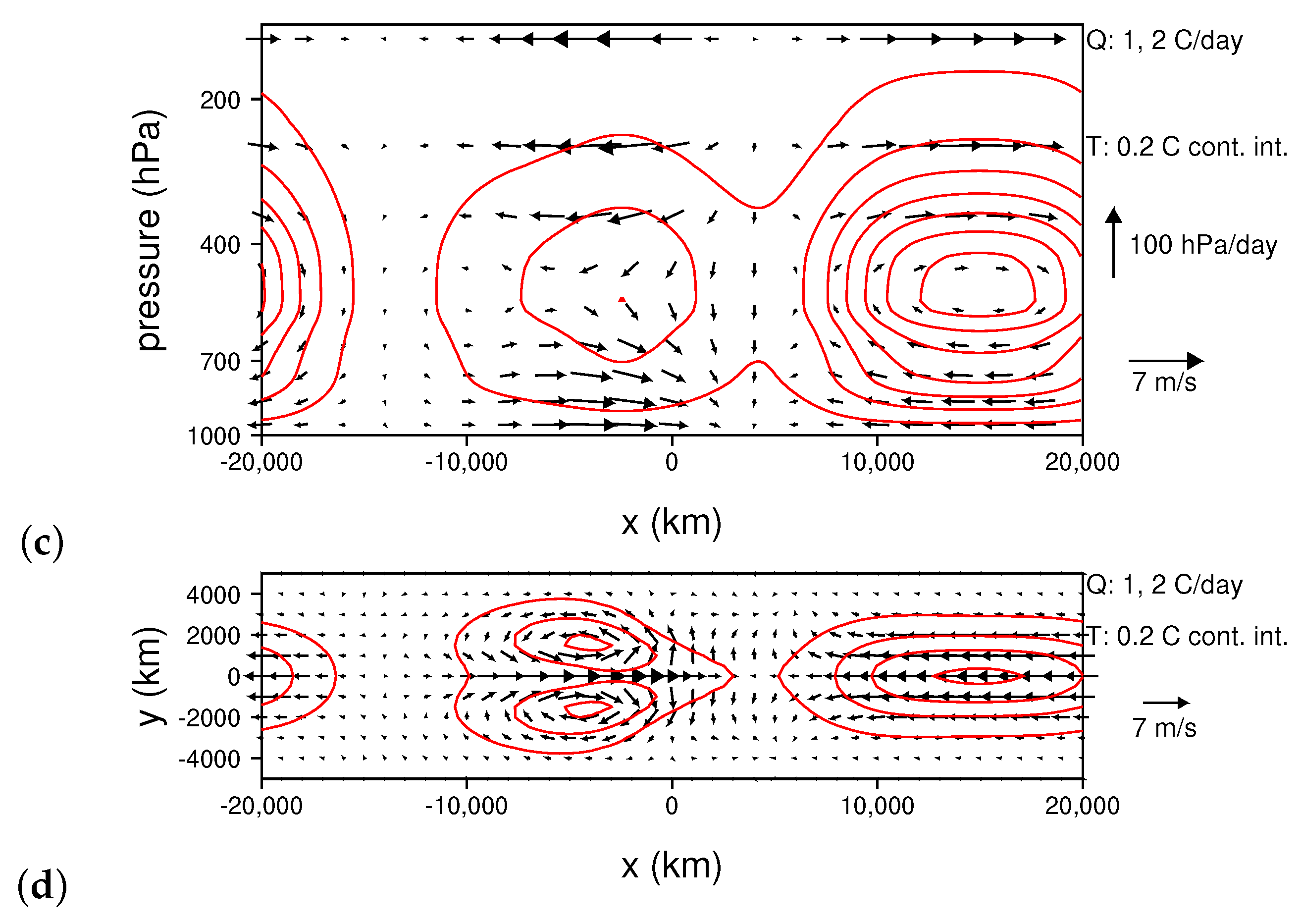
Figure 2 shows the linear “moist wave” response to a transient 3-day heating with the same vertical and horizontal structure as in the first simulation, but with a reduced amplitude. Note that, while we use the same wind vector scale as in Figure 1, the contour intervals for temperature and heating are reduced. In addition, note that we show the response for 7 days (instead of 5 days) in Figure 1c,d. There are several key differences from the dry wave response shown in Figure 1: (1) the amplitude of the temperature response is weaker, even though the amplitude of total (prescribed forcing + wave induced heating) is similar; (2) the moist waves propagate more slowly; and (3) the meridional extent of the waves is reduced. Surprisingly, despite the weaker forcing, the amplitude of horizontal wind perturbations is similar. The overall nature of the response is similar, as well, with a transient heating generating an eastward propagating Kelvin wave and westward propagating Rossby wave that separate after the heating is turned off.
3.1.3. Damped Moist Waves
In the simulations shown in Figure 1 and Figure 2, there is no dissipation, so that, after the forcing is turned off, the Kelvin and Rossby waves each propagate around the world and pass one another with little change in amplitude. This result stands in contrast to the classical Matsuno–Gill (Matsuno 1966; Gill 1980) solution of the atmospheric response to an equatorial heat source, which typically assumes a linear damping of momentum and/or temperature perturbations with a time scale of a few days. Figure 3 shows how our moist wave solution changes when such damping is included, and the heating is made to be permanent. After 3 h (Figure 3a), the solution has a similar structure to that for the inviscid simulation (Figure 2b) but with a weaker amplitude owing to the damping. By 12 h (Figure 3b), the solution is close to a steady state (i.e., it is essentially the same as the Matsuno-Gill solution). The Kelvin wave component (Figure 3c) extends farther east than the Rossby wave component extends west because the former propagates more rapidly. In this case, the distances that the Kelvin and Rossby waves extend from the heating depend on their phase speeds and the amplitude of linear damping, whereas, in the inviscid case, these distances increase with time as the wave fronts advance away from the heating.
As we note above, we choose a system of equations linearized about a basic state of rest with a rigid upper boundary immediately above the heating so that the dynamics reduce to those of a shallow water system (e.g., Reference [27,29]). Figure 4 shows that, for a heating with a spatial scale of the MJO, removing these assumptions primarily leads to a horizontal smoothing of mean tropospheric wave structures. For example, Figure 4a shows the effects of moving the upper boundary from 150 hPa to 25 hPa, which, when compared to Figure 1d, reveals that Kelvin and Rossby wave structures remain centered in roughly the same locations at time 5 h, but with slightly weaker amplitudes and broader meridional and zonal scales. As discussed by Reference [36], in this case, instead of projecting onto a single vertical mode, the heating excites a range of modes with varying equivalent depths, which disperse at slightly different phase speeds leading to an effective horizontal smoothing. Figure 4b shows the results of including non-linear terms, while still starting with a basic state of rest and using a high upper boundary, in a simulation conducted with the LAM. The results are very similar to the linear run with a high upper boundary (Figure 4a), suggesting that non-linear terms have second order effects. Figure 4c shows mean tropospheric wave structure at time 7 h for a non-linear run starting with the zonally symmetric wind field shown in Figure 5a, which is the zonal and annual mean of the flow in the LAM simulation we use to construct composite MJOs below. Note that this is a reasonable approximation of observed zonal and annual mean flow (Figure 5b). In this case, off-equatorial westerlies push the Rossby gyres slightly eastward, but Kelvin wave structure changes little from the run shown in Figure 4b. Taken together, these runs suggest that our simple linear system captures the basic dynamics of the equatorial atmosphere’s response to an MJO-like heating, but that using a more realistic system would yield an effective horizontal smoothing of wave structures and eastward advection of Rossby gyres.
3.2. Linear Atmospheric Response to Moving Heating and Cooling
In the previous section, we considered linear responses to stationary atmospheric heatings to illustrate some simple equatorial dynamics relevant to the dynamical interpretation of MJO circulation structure. We now consider a propagating heating and cooling that is more like those seen in MJOs in nature and general circulation models. For simplicity, we use a basic state of rest. Figure 6a shows a time longitude series of the heating used for the linear simulation presented in this section. It comprises three eastward propagating forcing components: a cooling followed by a heating and then another cooling. Each of these forcing functions are Gaussian with the same meridional and zonal scales as the stationary heating used in the previous section. The amplitude of the coolings are each 3/4 that of the heating. The heating function was constructed to mimic those of composite MJOs based on observations (Figure 6b) and simulations conducted with the LAM (Figure 6c). These observations and general circulation modeling results provide a means of evaluating to what extent the linear simulation captures circulations occurring in observed and/or modeled MJOs. In Figure 6a, we use colored lines to mark an approximate linear path of the positive heating anomaly, and we define the first third of this path as the developing stage, the middle third as the mature stage, and the last third as the dissipating stage. These stage definitions follow those of Reference [25,26] used for constructing composite observed and modeled MJOs. Below, we compare horizontal and vertical structures of wind and temperature perturbations for our linear model for each of these stages to corresponding structures of observed and simulated MJOs. Similar to the simulation presented in Section 3.1.2, we simulate a moist wave response here and use C/day, although here we assume 85 percent of the adiabatic temperature change due to vertical motion is canceled by convective heating.
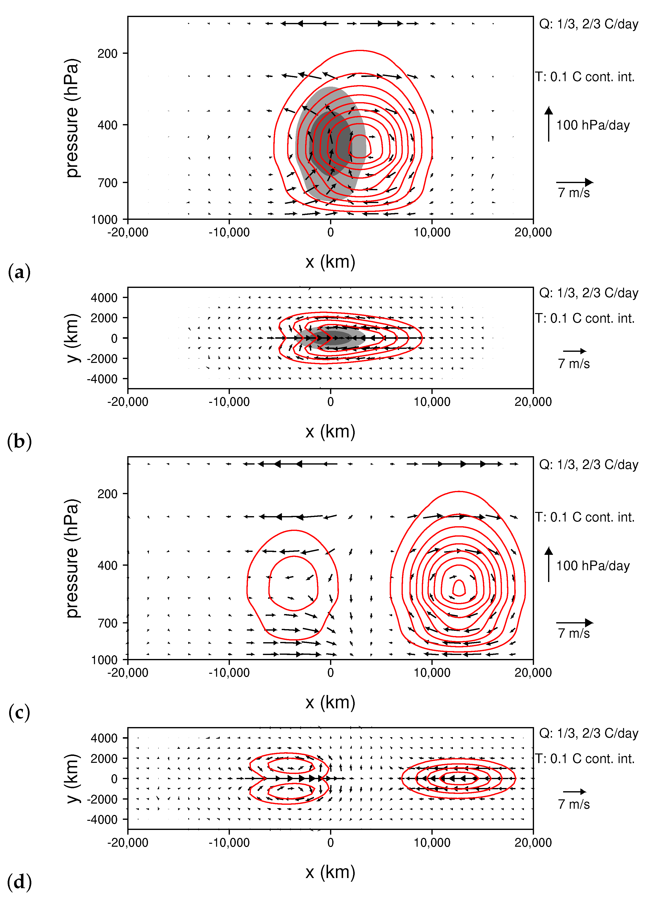
The horizontal structure of mean tropospheric temperature and wind shear perturbations (850 hPa minus 200 hPa flow) are shown for each of the developing, mature, and dissipating stages of the heating in Figure 7. For consistency with composite structures of observed and simulated MJOs, we compiled in previous studies (e.g., Reference [25,26]), we place all observations in a coordinate system that moves with the heating. For each stage, we provide the total temperature perturbation and flow field followed by the projection onto Kelvin waves followed by the residual when the Kelvin wave field is subtracted out, which generally resembles a Rossby Wave. During the developing stage, there is an equatorial Kelvin wave that spans halfway around the world originating within the cooling (light gray shading) and ending within the positive heating (dark shading; Figure 7a,b). This wave has a negative temperature perturbation and low-level westerly flow. There is also a smaller Kelvin wave growing eastward from the heating that includes a positive temperature perturbation and easterly low-level flow. The most prominent feature of the Rossby wave structure is a pair of anticylonic gyres with a negative temperature perturbation propagating westward from the negative heating anomaly (Figure 7c). Overall, the features seen in the developing stage (Figure 7a–c) are reminiscent of and largely predictable based on the simulation presented in Figure 2. As the cooling dissipates, it leaves a negative phase Kelvin wave propagating eastward from it (Figure 7a,b) and Rossby gyres propagating westward (Figure 7a,c). As the heating develops, a positive phase Kelvin wave begins propagating eastward from it (Figure 7b), as well as a positive phase Rossby wave propagating westward, which forms on top of and largely cancels out a portion of the negative phase Rossby wave previously generated by the cooling (Figure 7c).
During the developing stage of the heating, the negative phase Kelvin and Rossby waves diminish, and the positive phase waves grow (Figure 7d–f). For example, by the time the heating is near its peak, the positive phase Kelvin wave growing eastward from the heating is longer and stronger than the negative phase Kelvin wave entering the region of heating (Figure 7e). Since the waves are almost neutral (i.e., with no forcing they decrease in amplitude slowly owing to a 30-day damping), the vast majority of the change in the waves’ amplitudes occurs in response to the heating. As a negative phase wave enters the region of heating it is destroyed, and a positive wave grows out of the region of heating. Similarly, the negative phase Rossby wave diminishes as it propagates westward into the heating (Figure 7c,f), and a positive phase Rossby wave grows westward out of the heating (Figure 7f). The total positive temperature anomaly resembles a rocket at the mature stage(Figure 7d). By the dissipating stage, the equatorial warm anomaly, and accompanying low-level easterly flow have propagated almost all of the way around the world (Figure 7g,h). The Rossby gyres have grown and intensified when compared with the mature stage (Figure 7f,i). At this time, the cooling forming to the west of the heating has become almost as intense as the heating, and a cool-phase Kelvin wave is beginning to grow eastward out of it (Figure 7h).
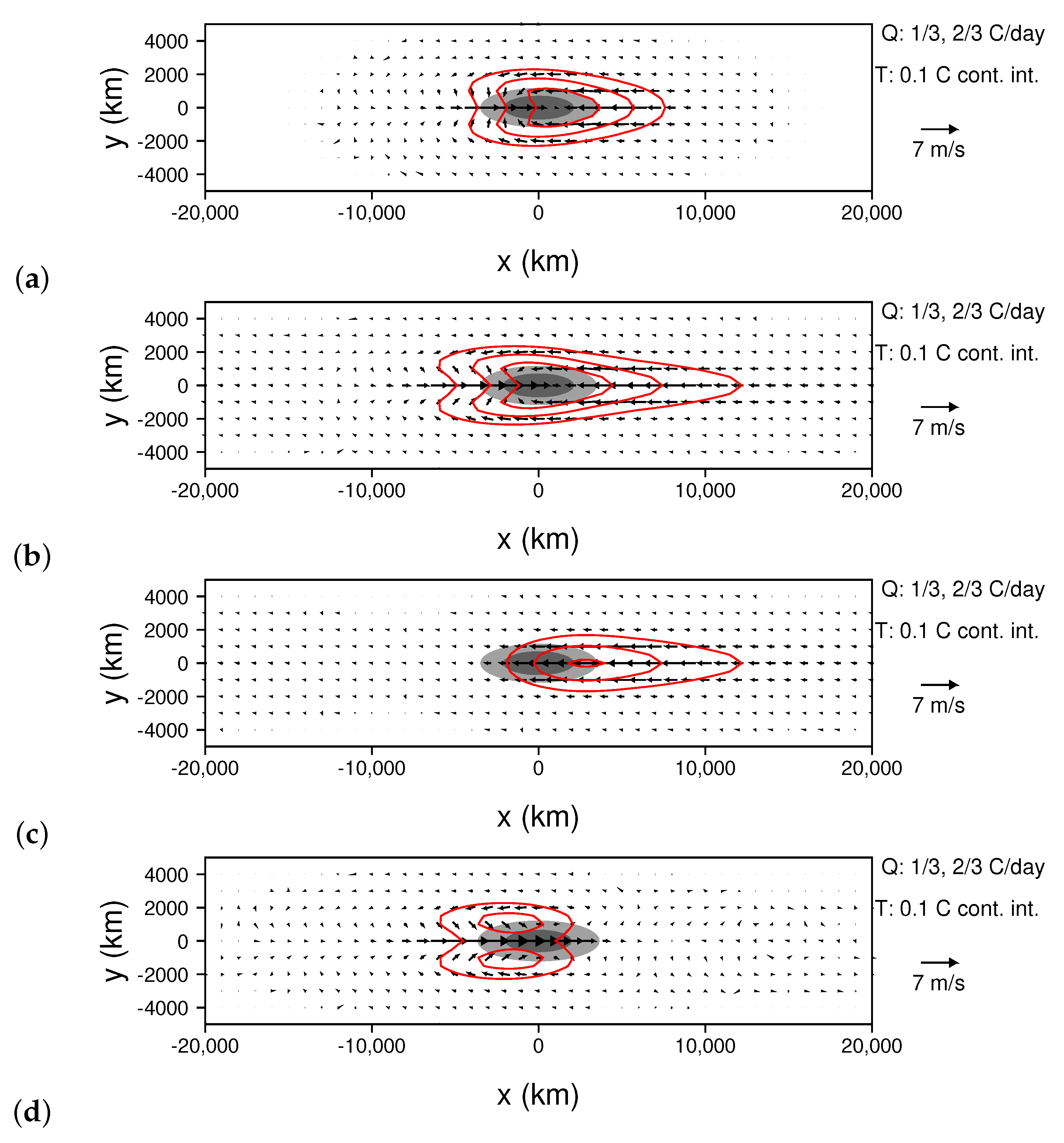
Figure 8 presents the same kind of analysis for the observed MJO; for each of the developing, mature, and dissipating stages, mean tropospheric temperature and 850–200 hPa wind shear are shown, followed by their projection onto Kelvin waves followed by the residual when the Kelvin wave fields are removed. During the developing stage, the positioning and phasing of equatorial Kelvin waves is similar to that in the linear simulation (Figure 8a,b). For example, in the Kelvin-filtered fields, a negative temperature perturbation accompanied by westerly low-level flow extends from just east of the cooling to the western edge of the heating (Figure 8b). This wave is also the dominant feature of the total flow to the west of the heating (Figure 8a). The observed MJO also has a positive phase Kelvin wave between the heating and cooling during the developing stage (Figure 8b). The Rossby waves with negative temperature perturbations in the observed MJO are displaced poleward and eastward of their counterparts in the linear simulation in the developing stage (compare Figure 7c and Figure 8c). This result can be expected based on the difference between the preliminary simulations with realistic zonal wind (Figure 4c) and with a resting basic stage (Figure 2d). However, the poleward displacement of Rossby waves is much more substantial in the observed MJO (Figure 8c), presumably because the forcing moves off the equator and the basic state meridional flow diverges at upper levels. This also means that the negative phase Rossby waves generated by the cooling to the east of the MJO do not move over the heating and that the growing positive phase Rossby waves just west of the heating can be discerned in the developing stage (Figure 8c), which is unlike the linear simulation (Figure 7c). During the developing and mature stages, the positive phase Kelvin wave grows until it stretches most of the way around the world (Figure 8h), with the same phasing relative to heating and cooling as in the linear simulation (Figure 7h). Rossby waves also intensify along the western flanks of the heating (Figure 8f,i), but they are farther east and displaced poleward relative to their counterparts in the linear simulation (Figure 7f,i).
Figure 9 presents a Kelvin-Rossby decomposition of a composite LAM MJO for each of the developing, mature, and dissipating stages of the convective envelope. Overall, it produces the same basic pattern of Kelvin and Rossby wave structure that is seen in the observations (Figure 8), and, in particular, generates Rossby waves that are farther east and off of the equator than those in the linear model (compare Figure 9c,f,i with Figure 7c,f,i). One reason for this could be that the model produces a v-shaped precipitation pattern on the western edge of the MJO (i.e., off-equatorial heating) that is also seen in observations (e.g., compare Figure 9f and Figure 8f). In both the model and nature, this could have something to do with cyclonic disturbances (e.g., twin cyclones) breaking off of the western edge of the MJO (e.g., Reference [37]). The author is unaware of other studies that have systematically partitioned MJO circulation structure generated by a general circulation model into Kelvin and Rossby waves, so it is hard to say how the LAM’s reproduction of this structure compares to that in other models.
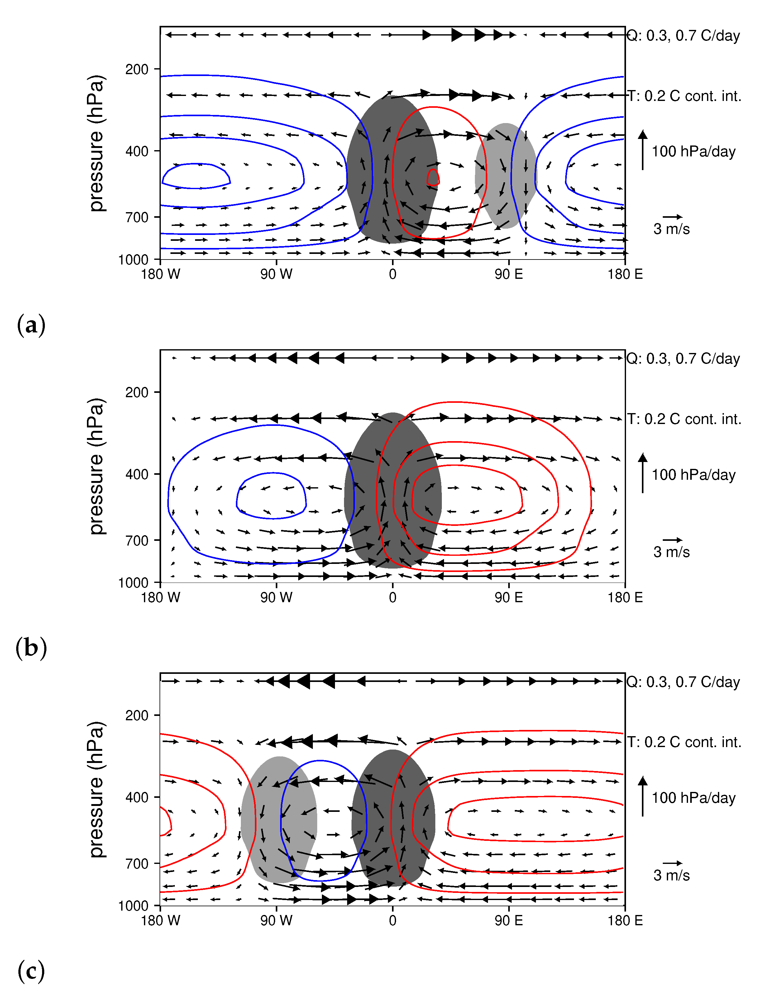
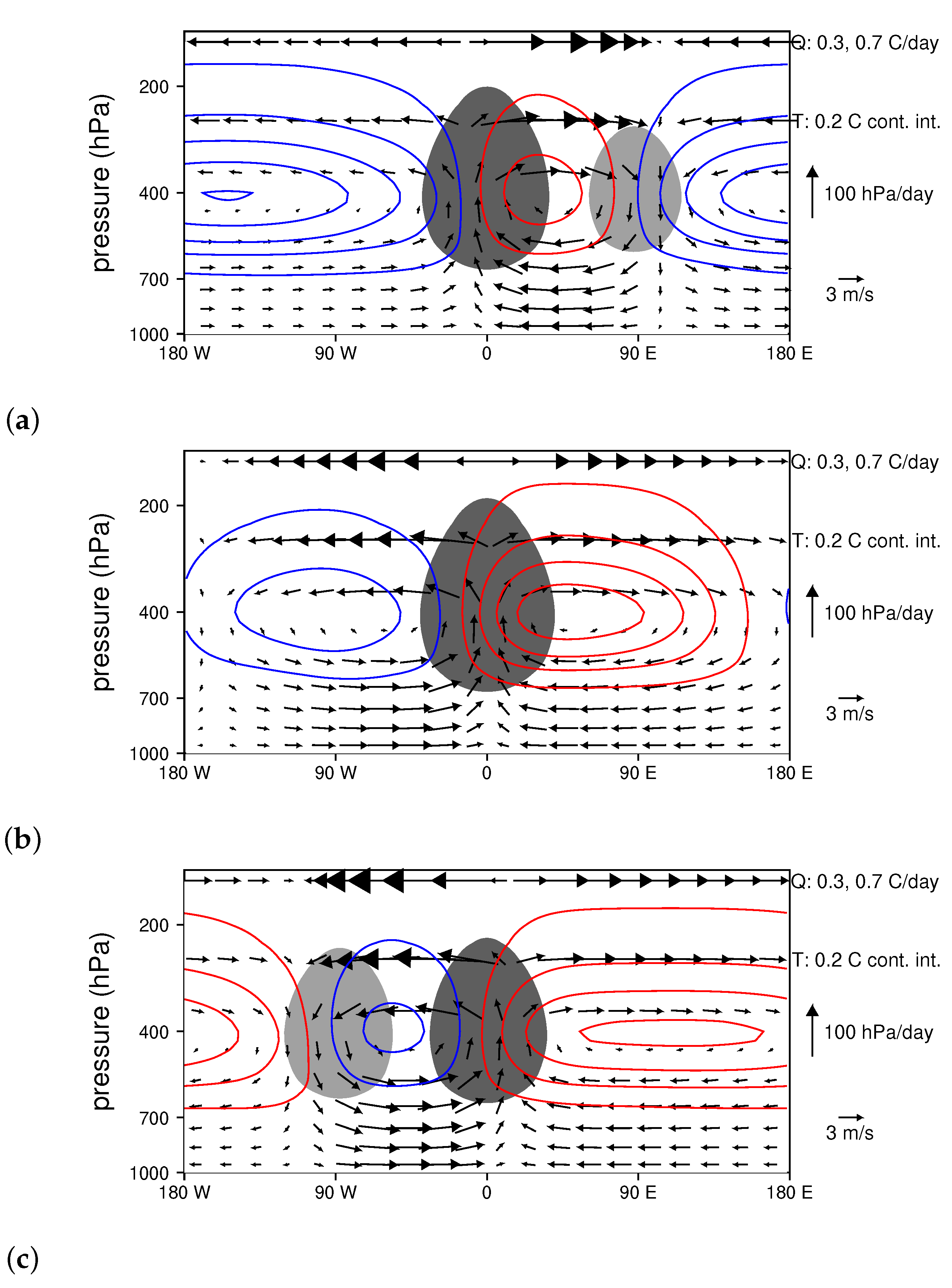
East-west vertical cross-sections of temperature and wind perturbations along the equator are shown for each of the developing, mature, and dissipating stages of the heating in the linear simulation in Figure 10. When the heating is developing, a warm anomaly extends about 70 degrees eastward from its center, which is co-located with strong low-level (upper-level) easterly (westerly) wind perturbations (Figure 10a). The remainder of the troposphere is cool with opposite sign wind perturbations (Figure 10a), which is the signature the equatorial Kelvin wave that has propagated most of the way around the world originating from the cooling that preceded the heating (Figure 7b). By the time the heating is near its peak, the warm anomaly and accompanying low-level (upper-level) easterlies (westerlies) have expanded eastward, reaching almost halfway around the world (Figure 10b). By this time, the cooling has largely dissipated, and the western edge of the Kelvin wave that originated from the cooling has also advanced eastward. When the heating is dissipating, the warm Kelvin wave has spread most of the warm around the world, and the negative temperature perturbation spans only about 70 degrees of longitude (Figure 10a). Overall, the temperature signal at the equator is dominated by the Kelvin wave component (Figure 7b,e,h), with the Rossby waves primarily enhancing low-level (upper-level) easterlies (westerlies) to the east of the heating in the developing stage (Figure 6c and Figure 10a), and low-level (upper-level) westerlies (easterlies) to the west of the heating in the mature and dissipating stages (Figure 7f,i and Figure 10b,c).
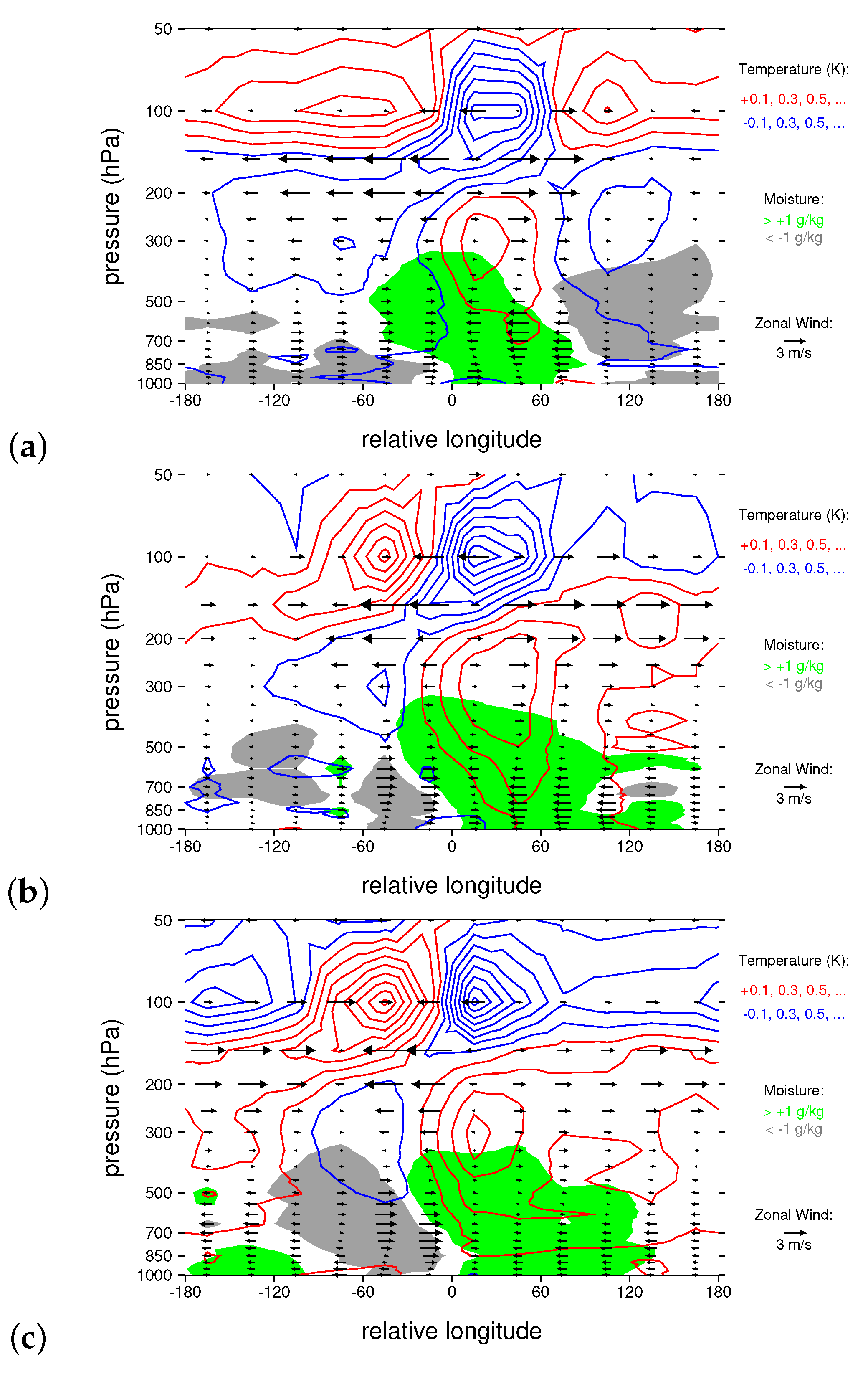
The observed tropospheric structure of the MJO (Figure 11) has the same basic pattern as that simulated by the linear model. During the developing stage, most of the troposphere is cool with low-level westerlies and upper-level easterlies, but there is a small warm anomaly just east of the convective center with the opposite wind pattern (Figure 11a). The warm anomaly and low-level easterlies and upper-level westerlies expand eastward during the mature and dissipating stages until they cover most of the equatorial belt (Figure 11b,c). The main difference between observed and simulated vertical structures is that the peak temperature perturbation and transition from easterlies to westerlies occur higher in nature (300 hPa) than they do in the linear model (500 hPa; compare Figure 10 and Figure 11). As we discuss in more detail below, this is likely a consequence of excluding the “stratiform” component of convective heating (Mapes and Houze, 1995), and the linear model can easily be modified to produce a more realistic temperature peak and wind transition. Another way that the observed MJO vertical structure differs from that in the linear model is that during the mature and dissipating stages the temperature anomaly rises to the east of the convective center, suggesting vertical wave propagation (Figure 11b,c). Vertical wave propagation is excluded in our simple model owing to the rigid lid above the heating, which is necessary for retaining an isomorphism to shallow water dynamics. The simple model also excludes topographic variations, which could contribute differences between the observed and modeled MJO.
The LAM reproduces the key differences between the linear simulation and the observed MJO, including higher peak temperature anomalies and transitions between easterlies and westerlies (Figure 12). The model also generates lower stratospheric temperature anomalies that are out of phase with tropospheric anomalies, as well as vertical wave propagation connecting some tropospheric and lower-stratospheric perturbations (compare Figure 11 and Figure 12). Low-level temperature anomalies in the LAM are stronger than they are in nature, suggesting that the model may be lacking some low-level dissipative processes.
The problem of local maxima in temperature and wind direction changes occurring too low in the linear model has a reasonable fix with a physical explanation. It has long been known that, owing to the effects of convectively generated stratiform precipitation, deep convective heating in the tropics is typically more top heavy than that for the first vertical mode (e.g., Reference [38]). Especially for high frequency tropical disturbances, such as 2-day waves, it has been popular to interpret and model wave circulations using 2 vertical modes (e.g., Reference [27,39,40]. For such short time scales, there is little doubt that these two modes are often substantially out of phase, leading to strong tilts in wind and temperature perturbations. In contrast, it remains an open question as to whether two separate modes are required to capture the dynamics of the MJO, which often has less pronounced tilts in wind, temperature, and heating perturbations (e.g., Figure 11). In Figure 13, we show how the vertical structure of the linear response to the MJO-like heating is changed when the second vertical mode is added to the heating to make it more top heavy. Here, we use a weaker partial cancellation of adiabatic temperature changes due to vertical motion for the 2nd mode, which is consistent with observations [28], so that that two modes have the same equivalent depth (also see Reference [27]). While the horizontal structure of simulated Kelvin and Rossby waves changes little (not shown), local minima and maxima in temperature perturbations move higher in the troposphere, as does the transition level between easterlies and westerlies (compare Figure 10 and Figure 13). The net result is that the simple model produces a reasonable approximation of observed MJO vertical structure for each of the developing, mature, and dissipating stages (compare Figure 11 and Figure 13).
4. Summary and Discussion
In this paper, we decompose MJO circulations into Kelvin and Rossby wave components for three sets of data: (1) a modeled linear response to an MJO-like heating; (2) a composite MJO based on atmospheric sounding data; and (3) a composite MJO based on data from a Lagrangian atmospheric model. The first dataset is governed by the the shallow water equations on a beta-plane linearized about a basic state of rest; therefore, it has the cleanest and most straightforward projection onto Kelvin and Rossby waves, as well as the simplest dynamical interpretation. The second system provides a realistic view of MJO circulations, and it is constructed in a frame of reference that moves with the MJO’s heating, and without any contamination from model output. The third dataset, which which provides a picture of MJO circulation and decomposition that is consistent with observations, has additional features, such as a uniform sampling of data, precise heating, and surface flux information, and it is created in a laboratory in which controlled experiments can be conducted.
In all three of the datasets, the propagation of Kelvin waves is similar. During the developing stage, an equatorial Kelvin wave with a negative tropospheric temperature perturbation and low-level westerly wind perturbations spans most of the equatorial belt, originating in a region of convective cooling to the east of the MJO and ending in the MJO’s convective heating (Figure 7b, Figure 8b, and Figure 9b). During the mature stage, this wave contracts as a positive phase Kelvin wave with low-level easterlies grows out of the east side of the convective heating (Figure 7e, Figure 8e and Figure 9e). This wave eventually wraps most of the way around the world, terminating in a convectively suppressed region to the west of the MJO (Figure 7h, Figure 8h, Figure 9h). The close similarity between the phasing of the Kelvin waves in the observed MJO and the linear simulation suggests that the dynamics of Kelvin wave circulations in the MJO can be captured by a system of equations linearized about a basic state of rest, and this also supports the use of such systems for theoretical interpretations of the Kelvin wave component of the MJO’s circulation (e.g., Reference [21]). Note also that Kelvin wave low-level convergence, which implies upward motion, is coincident with the growth of MJO convection, a point noted by a number of previous studies (Figure 7b, Figure 8b and Figure 9b, e.g., Reference [25,41]). It is also quite possible that Kelvin wave low-level divergence that occurs after the warm phase wave has circumnavigated the globe (Figure 7h, Figure 8h and Figure 9h) contributes to the development of the suppressed phase of the MJO.
In contrast, the Rossby wave component of the MJO’s circulation in the observations and the LAM behave somewhat differently that that in the linear model. In the linear model, Rossby gyres remain close to the equator and move directly westward from the forcing (Figure 7c,f,i), but, in the observations and the LAM, the gyres form on the western flank of the heating and move along with the heating, which propagates eastward around 5 m/s (Figure 8f,i and Figure 9c,f,i). This leads to a broader and weaker swath of equatorial westerlies that is displaced eastward when compared with those in the linear model (e.g., compare Figure 7f and Figure 8f). This result suggests that the use of a system of equations linearized about a basic state of rest for the theory and modeling of the Rossby component of the MJO’s circulation will lead to substantial errors in circulation and terms derived from circulations, such as surface fluxes and advection of moisture. Previous studies have noted how the presence of a zonal jet distorts the Rossby wave component of MJO circulation (e.g., Reference [42,43]) and produces Rossby gyres centered farther off the equator than those occuring in a basic state of rest. However, our sensitivity test with a realistic zonal wind field (Figure 2d) suggests this leads to more of an eastward shift in the Rossby gyre as opposed to a poleward shift. Perhaps other factors, such as advection by the basic state meridional flow and the tendency of the MJO to shed tropical cyclones that propagate poleward, are also contributing to the poleward shift of Rossby gyres in the composite observed and LAM MJOs (Figure 8f,i and Figure 9f,i).
The dynamical analysis of the life-cycle of MJO circulations presented in this paper stands in stark contrast that in the classical Matsuno–Gill model (MG) [30,44]. In the MG model, owing strong linear dissipation, there is a steady-state response to an equatorial heating that includes a Kelvin wave to the east of the heating and a Rossby wave to the west, with the distance that each wave extends from the heating roughly proportional to the propagation speed of the wave divided by the time scale of damping (Figure 3b). In the linear model used here, the Kelvin waves circumnavigate the globe owing to very weak 30-day damping, and there is a strong sloshing of wave circulations with significant differences in different stages of the life cycle (i.e, the solution is far from a steady state). Moreover, the simulations presented here highlight the importance of negative forcing in generating the cool phase Kelvin wave that enters the MJO during the developing stage of convection, as well as the upper-level quadrapole of the MJO (e.g., Reference [7]). Roundy [45] also noticed a zonally broad negative 200 hPa height anomaly (consistent with a cool troposphere) lying to the west of the convectively active region of the MJO (see his Figure 3c), which is likely a signature of the cool phase Kelvin wave discussed here.
While this study helps to quantify the contribution of Kelvin and Rossby waves to the MJO’s horizontal circulation, it also leaves many questions unanswered. For example, do other general circulation models besides the LAM properly partition circulations between Kelvin and Rossby waves for different stages of the MJO’s convective life cycle? How do each of the two wave types contribute to surface fluxes, moisture tranport, and other aspects of the mechanism of the MJO? Will the relative strengths of Kelvin and Rossby components change in a changing climate? The author hopes to be able to address these questions with future applications of the Kelvin/Rossby decomposition method used here.
Funding
This research was supported by NSF grant AGS-1561066.
Data Availability Statement
Data for the linear simulation with a moving MJO-like heat source (Section 3.2), which is the new data created for this paper that supports the key conclusions, is available at http://ducky.net/lom/dat_mv.zip.
Conflicts of Interest
The authors declare no conflict of interest.
Appendix A. The Kelvin Wave Projection Algorithm
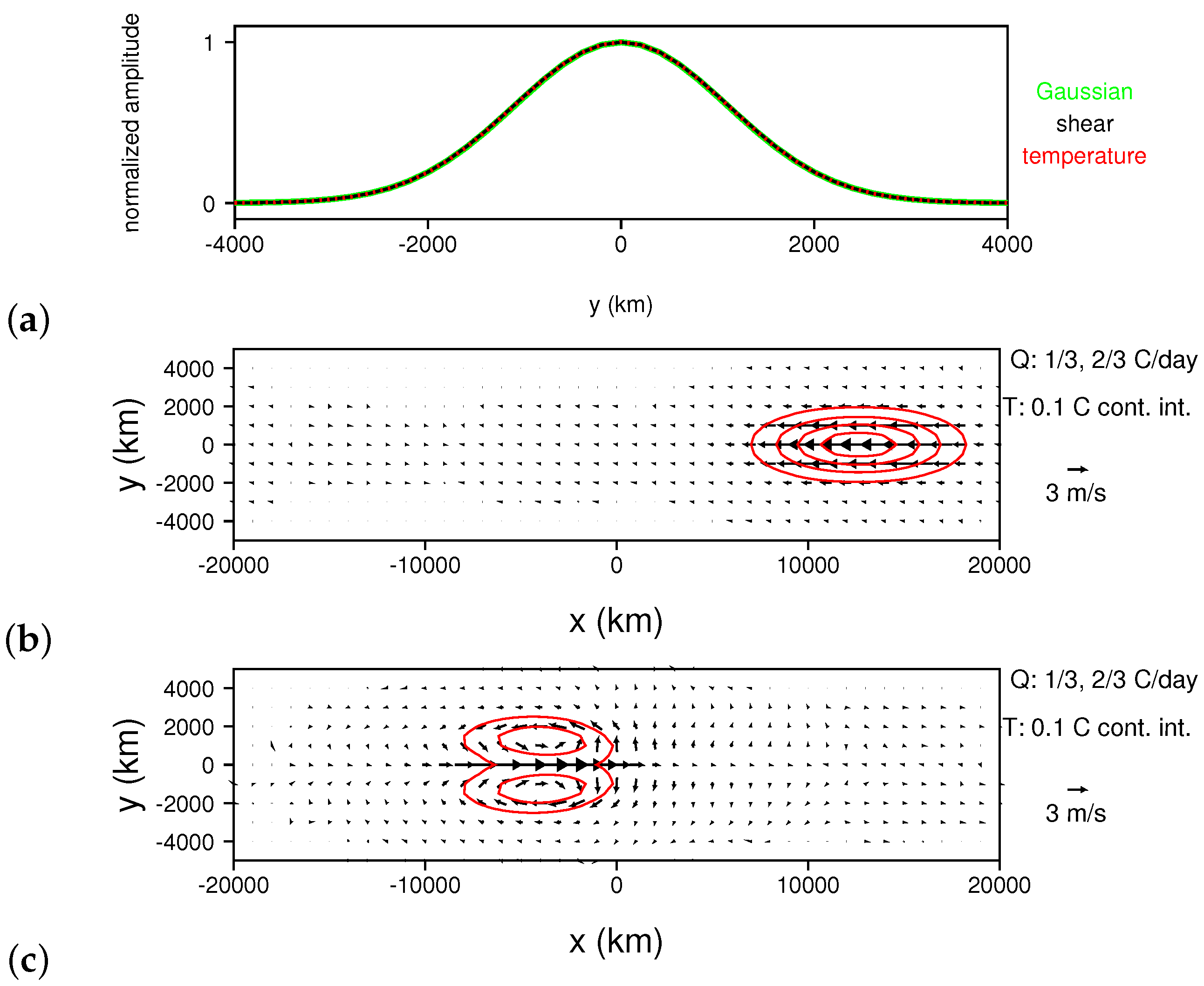
In this paper, we employ a method of separating Kelvin and Rossby wave circulations that is developed for simulations conducted with our linear model, and modified to apply to observed MJOs, as well as those simulated with the Lagrangian Atmospheric Model (LAM). Kelvin waves excited by a heat source in our linear model have meridional structures that closely follow those predicted by linear theory. For example, in Figure A1a, we plot the theoretical meridional structure function for a Kelvin wave, which is a Guassian, as well as the meridional structures of mean tropospheric temperature (T) and 850 hPa minus 200 hPa zonal flow (S). Modeled perturbations are along km at days for the simulation presented in Section 3.1.2 (also see Figure 2a,b). All three curves in Figure A1a are normalized by dividing by the maximum value, so it becomes clear that each has the same meridional structure, which is that for a pure Kelvin wave with a meridional length scale km. By comparing the normalization constants, we determine that the ratio of zonal wind shear perturbations to mean tropospheric temperature perturbations in Kelvin waves in our linear model is m/s/C. We use this information to define a Kelvin wave projection:
where k is the coefficient of the Kelvin wave projection, and y is non-dimensional distance from the equator, with the Kelvin-wave projected fields given by
The results of applying this projection to the (S,T) fields for days (Figure 2d) are shown in Figure A1b. The projection successfully preserves the Kelvin wave while removing the Rossby wave. When the Kelvin wave projected fields are removed from the total fields, the residual field is dominated by the Rossby wave (Figure A1c). While we tested this method for a case in which Kelvin and Rossby waves have separated, it is most useful when they overlap as in the MG solution (Figure 3), the linear simulation with moving heating and cooling (Figure 7), and in observed and simulated MJO fields (Figure 8 and Figure 9). For the latter, we found it helpful to reduce the value of r to 12 m/s/C as the ratio of shear to mean troposheric temperature is lower in observed and simulated MJOs than in the linear simulation (e.g., compare Figure 10, Figure 11 and Figure 12). For the simulation presented in Section 3.2, we used an enhanced cancellation of adiabatic temperature changes by convective heating (85 percent instead of the 70 percent used in Section 3.1.2 and Section 3.1.3), which leads to m/s/C and km for simulated Kelvin waves.
Figure A1.
Illustration of the Kelvin wave projection algorithm. (a) The theoretical meridional structure for a Kelvin wave (green), as well as normalized meridional structures of mean tropospheric temperature (red dots) and 850–200 hPa zonal wind shear along km at days for the linear simulation shown in Figure 2. (b) Kelvin wave projected mean tropospheric temperature and 850–200 hPa wind shear for days. (c) Residual fields when the Kelvin wave structure is removed at days. Panels (b,c) are contoured as in Figure 2b,d. Comparing panels (b,c) to Figure 2d reveals that the method successfully partitions Kelvin and Rossby wave circulations.

References
- Madden, R.A.; Julian, P.R. Detection of a 40–50 day oscillation in the zonal wind in the tropical Pacific. J. Atmos. Sci. 1971, 28, 702–708. [Google Scholar] [CrossRef]
- Madden, R.A.; Julian, P.R. Description of global-scale circulation cells in the tropics with a 40–50 day period. J. Atmos. Sci. 1972, 29, 1109–1123. [Google Scholar] [CrossRef]
- Madden, R.A.; Julian, P.R. Observations of the 40–50-day tropical oscillation—A review. Mon. Weather. Rev. 1994, 122, 814–837. [Google Scholar] [CrossRef]
- Nakazawa, T. Tropical super clusters within intraseasonal variations over the western Pacific. J. Meteorol. Soc. Jpn. Ser. II 1988, 66, 823–839. [Google Scholar] [CrossRef] [Green Version]
- Hendon, H.H.; Liebmann, B. Organization of convection within the Madden-Julian oscillation. J. Geophys. Res. Atmos. 1994, 99, 8073–8083. [Google Scholar] [CrossRef]
- Takayabu, Y.N.; Lau, K.; Sui, C. Observation of a quasi-2-day wave during TOGA COARE. Mon. Weather. Rev. 1996, 124, 1892–1913. [Google Scholar] [CrossRef] [Green Version]
- Kiladis, G.N.; Straub, K.H.; Haertel, P.T. Zonal and vertical structure of the Madden–Julian oscillation. J. Atmos. Sci. 2005, 62, 2790–2809. [Google Scholar] [CrossRef]
- Wheeler, M.; Kiladis, G.N. Convectively coupled equatorial waves: Analysis of clouds and temperature in the wavenumber–frequency domain. J. Atmos. Sci. 1999, 56, 374–399. [Google Scholar] [CrossRef]
- Maloney, E.D.; Hartmann, D.L. Modulation of eastern North Pacific hurricanes by the Madden–Julian oscillation. J. Clim. 2000, 13, 1451–1460. [Google Scholar] [CrossRef]
- Liebmann, B.; Hendon, H.H.; Glick, J.D. The relationship between tropical cyclones of the western Pacific and Indian Oceans and the Madden-Julian oscillation. J. Meteorol. Soc. Jpn. Ser. II 1994, 72, 401–412. [Google Scholar] [CrossRef] [Green Version]
- Wu, M.L.C.; Schubert, S.; Huang, N.E. The development of the South Asian summer monsoon and the intraseasonal oscillation. J. Clim. 1999, 12, 2054–2075. [Google Scholar] [CrossRef]
- Lorenz, D.J.; Hartmann, D.L. The effect of the MJO on the North American monsoon. J. Clim. 2006, 19, 333–343. [Google Scholar] [CrossRef] [Green Version]
- Haertel, P.; Boos, W.R. Global association of the Madden-Julian Oscillation with monsoon lows and depressions. Geophys. Res. Lett. 2017, 44, 8065–8074. [Google Scholar] [CrossRef]
- Emanuel, K.A. An air-sea interaction model of intraseasonal oscillations in the tropics. J. Atmos. Sci. 1987, 44, 2324–2340. [Google Scholar] [CrossRef] [Green Version]
- Sobel, A.; Maloney, E. An idealized semi-empirical framework for modeling the Madden–Julian oscillation. J. Atmos. Sci. 2012, 69, 1691–1705. [Google Scholar] [CrossRef]
- Wang, B.; Rui, H. Dynamics of the coupled moist Kelvin–Rossby wave on an equatorial β-plane. J. Atmos. Sci. 1990, 47, 397–413. [Google Scholar] [CrossRef] [Green Version]
- Maloney, E.D.; Hartmann, D.L. Frictional moisture convergence in a composite life cycle of the Madden-Julian oscillation. J. Clim. 1998, 11, 2387–2403. [Google Scholar] [CrossRef]
- Raymond, D.J. A new model of the Madden–Julian oscillation. J. Atmos. Sci. 2001, 58, 2807–2819. [Google Scholar] [CrossRef]
- Straus, D.M.; Lindzen, R.S. Planetary-scale baroclinic instability and the MJO. J. Atmos. Sci. 2000, 57, 3609–3626. [Google Scholar] [CrossRef]
- Biello, J.A.; Majda, A.J.; Moncrieff, M.W. Meridional momentum flux and superrotation in the multiscale IPESD MJO model. J. Atmos. Sci. 2007, 64, 1636–1651. [Google Scholar] [CrossRef] [Green Version]
- Zhang, C.; Adames, Á.; Khouider, B.; Wang, B.; Yang, D. Four Theories of the Madden-Julian Oscillation. Rev. Geophys. 2020, 58, e2019RG000685. [Google Scholar] [CrossRef] [PubMed]
- Hung, M.P.; Lin, J.L.; Wang, W.; Kim, D.; Shinoda, T.; Weaver, S.J. MJO and convectively coupled equatorial waves simulated by CMIP5 climate models. J. Clim. 2013, 26, 6185–6214. [Google Scholar] [CrossRef]
- Jiang, X.; Waliser, D.E.; Xavier, P.K.; Petch, J.; Klingaman, N.P.; Woolnough, S.J.; Guan, B.; Bellon, G.; Crueger, T.; DeMott, C.; et al. Vertical structure and physical processes of the Madden-Julian oscillation: Exploring key model physics in climate simulations. J. Geophys. Res. Atmos. 2015, 120, 4718–4748. [Google Scholar] [CrossRef]
- Ahn, M.S.; Kim, D.; Kang, D.; Lee, J.; Sperber, K.R.; Gleckler, P.J.; Jiang, X.; Ham, Y.G.; Kim, H. MJO Propagation across the Maritime Continent: Are CMIP6 Models Better than CMIP5 Models? Geophys. Res. Lett. 2020, e2020GL087250. [Google Scholar] [CrossRef]
- Haertel, P.; Straub, K.; Budsock, A. Transforming circumnavigating Kelvin waves that initiate and dissipate the Madden–Julian Oscillation. Q. J. R. Meteorol. Soc. 2015, 141, 1586–1602. [Google Scholar] [CrossRef]
- Haertel, P.; Boos, W.R.; Straub, K. Origins of Moist Air in Global Lagrangian Simulations of the Madden–Julian Oscillation. Atmosphere 2017, 8, 158. [Google Scholar] [CrossRef] [Green Version]
- Haertel, P.T.; Kiladis, G.N. Dynamics of 2-day equatorial waves. J. Atmos. Sci. 2004, 61, 2707–2721. [Google Scholar] [CrossRef]
- Haertel, P.T.; Kiladis, G.N.; Denno, A.; Rickenbach, T.M. Vertical-mode decompositions of 2-day waves and the Madden–Julian oscillation. J. Atmos. Sci. 2008, 72. [Google Scholar] [CrossRef]
- Fulton, S.R.; Schubert, W.H. Vertical normal mode transforms: Theory and application. Mon. Weather. Rev. 1985, 113, 647–658. [Google Scholar] [CrossRef] [Green Version]
- Matsuno, T. Quasi-geostrophic motions in the equatorial area. J. Meteorol. Soc. Jpn. Ser. II 1966, 44, 25–43. [Google Scholar] [CrossRef] [Green Version]
- Haertel, P.T.; Straub, K.H. Simulating convectively coupled Kelvin waves using Lagrangian overturning for a convective parametrization. Q. J. R. Meteorol. Soc. 2010, 136, 1598–1613. [Google Scholar] [CrossRef]
- Haertel, P.; Straub, K.; Fedorov, A. Lagrangian overturning and the Madden–Julian Oscillation. Q. J. R. Meteorol. Soc. 2014, 140, 1344–1361. [Google Scholar] [CrossRef]
- Haertel, P. A Lagrangian method for simulating geophysical fluids. In Lagrangian Modeling of the Atmosphere; Yale University: New Haven, CT, USA, 2012; pp. 85–98. [Google Scholar]
- Haertel, P. Sensitivity of the Madden Julian Oscillation to Ocean Warming in a Lagrangian Atmospheric Model. Climate 2018, 6, 45. [Google Scholar] [CrossRef] [Green Version]
- Haertel, P. Prospects for Erratic and Intensifying Madden-Julian Oscillations. Climate 2020, 8, 24. [Google Scholar] [CrossRef] [Green Version]
- Mapes, B.E. The large-scale part of tropical mesoscale convective system circulations. J. Meteorol. Soc. Jpn. Ser. II 1998, 76, 29–55. [Google Scholar] [CrossRef] [Green Version]
- Ferreira, R.N.; Schubert, W.H.; Hack, J.J. Dynamical aspects of twin tropical cyclones associated with the Madden–Julian oscillation. J. Atmos. Sci. 1996, 53, 929–945. [Google Scholar] [CrossRef] [Green Version]
- Mapes, B.E.; Houze, R.A., Jr. Diabatic divergence profiles in western Pacific mesoscale convective systems. J. Atmos. Sci. 1995, 52, 1807–1828. [Google Scholar] [CrossRef] [Green Version]
- Khouider, B.; Majda, A.J. Model multi-cloud parameterizations for convectively coupled waves: Detailed nonlinear wave evolution. Dyn. Atmos. Ocean. 2006, 42, 59–80. [Google Scholar] [CrossRef]
- Kuang, Z. A moisture-stratiform instability for convectively coupled waves. J. Atmos. Sci. 2008, 65, 834–854. [Google Scholar] [CrossRef]
- Powell, S.W.; Houze, R.A., Jr. Effect of dry large-scale vertical motions on initial MJO convective onset. J. Geophys. Res. Atmos. 2015, 120, 4783–4805. [Google Scholar] [CrossRef]
- Monteiro, J.M.; Adames, Á.F.; Wallace, J.M.; Sukhatme, J.S. Interpreting the upper level structure of the Madden-Julian oscillation. Geophys. Res. Lett. 2014, 41, 9158–9165. [Google Scholar] [CrossRef] [Green Version]
- Adames, Á.F.; Wallace, J.M. Three-dimensional structure and evolution of the MJO and its relation to the mean flow. J. Atmos. Sci. 2014, 71, 2007–2026. [Google Scholar] [CrossRef]
- Gill, A. Some simple solutions for heat-induced tropical circulation. Q. J. R. Meteorol. Soc. 1980, 106, 447–462. [Google Scholar] [CrossRef]
- Roundy, P.E. Interpretation of the spectrum of eastward-moving tropical convective anomalies. Q. J. R. Meteorol. Soc. 2020, 146, 795–806. [Google Scholar] [CrossRef]
Figure 1.
The dry atmospheric response to a stationary and transient Madden Julian Oscillation (MJO)-like heating. Temperature is contoured with a 0.2 C interval (0.1, 0.3, 0.5, … C), and vectors indicate wind flow. Light shading indicates heating greater than 1 C/day, and dark shading shows heating greater than 2 C/day. Panels (a,c) are vertical cross-sections along the equator at 3 and 5 days, respectively, and panels (b,d) show mean tropospheric temperature and the difference between 850 hPa and 200 hPa horizontal flow for 3 and 5 days, respectively.


Figure 2.
The “moist” atmospheric response to a stationary and transient MJO-like heating. Temperature is contoured with a 0.1 C interval (0.1, 0.2, 0.3, … C), and vectors indicate wind flow. Light shading indicates heating greater than 1/3 C/day, and dark shading indicates heating greater that 2/3 C/day. Panels (a,c) are vertical cross-sections along the equator at 3 and 7 days, respectively, and panels (b,d) show mean tropospheric temperature and the difference between 850 hPa and 200 hPa horizontal flow for 3 and 7 days, respectively.

Figure 3.
The “moist” atmospheric response to a stationary MJO-like heating with 3-day linear damping. Temperature is contoured with a 0.1 C interval (0.1, 0.2, 0.3, … C), and vectors indicate wind flow. Light shading indicates heating greater than 1/3 C/day, and dark shading indicates heating greater than 2/3 C/day. Panels (a,b) show mean tropospheric temperature and the difference between 850 hPa and 200 hPa horizontal flow for 3 and 12 days, respectively, and panels (c,d) show the projection of the solution at 12 days onto Kelvin and Rossby waves, respectively.

Figure 4.
Sensitivity of the dry wave response at 5 h (Figure 1d) to changes in the model. (a) A simulation with the upper boundary moved to 25 hPa. (b) A fully non-linear simulation with a higher upper boundary starting with a basic state of rest. (c) A nonlinear simulation with a realistic zonal flow. In each panel, average tropospheric temperature is contoured with a 0.1 C interval (0.1, 0.2, 0.3 C), and vectors indicate the difference between 850 hPa and 200 hPa horizontal The simulation in panel (a) is conducted with the linear model, and the simulations shown in panels (b,c) are conducted with the Lagrangian Atmospheric Model (LAM).

Figure 5.
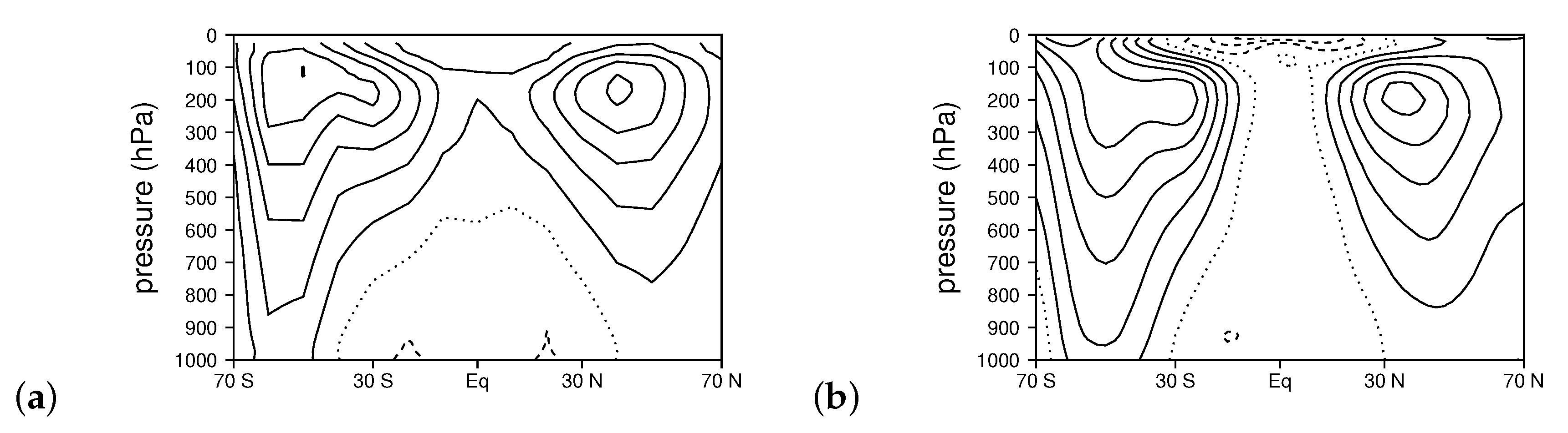
The initial zonal flow for the sensitivity test with a non-resting basic state (a) compared with the observed zonal and annual mean zonal flow from the National Center for Environmental Prediction reanalysis (b). In each panel, zonal flow is contoured with a 5 m/s interval, the zero contour is dotted, and negative contours are dashed.
Figure 5.
The initial zonal flow for the sensitivity test with a non-resting basic state (a) compared with the observed zonal and annual mean zonal flow from the National Center for Environmental Prediction reanalysis (b). In each panel, zonal flow is contoured with a 5 m/s interval, the zero contour is dotted, and negative contours are dashed.

Figure 6.
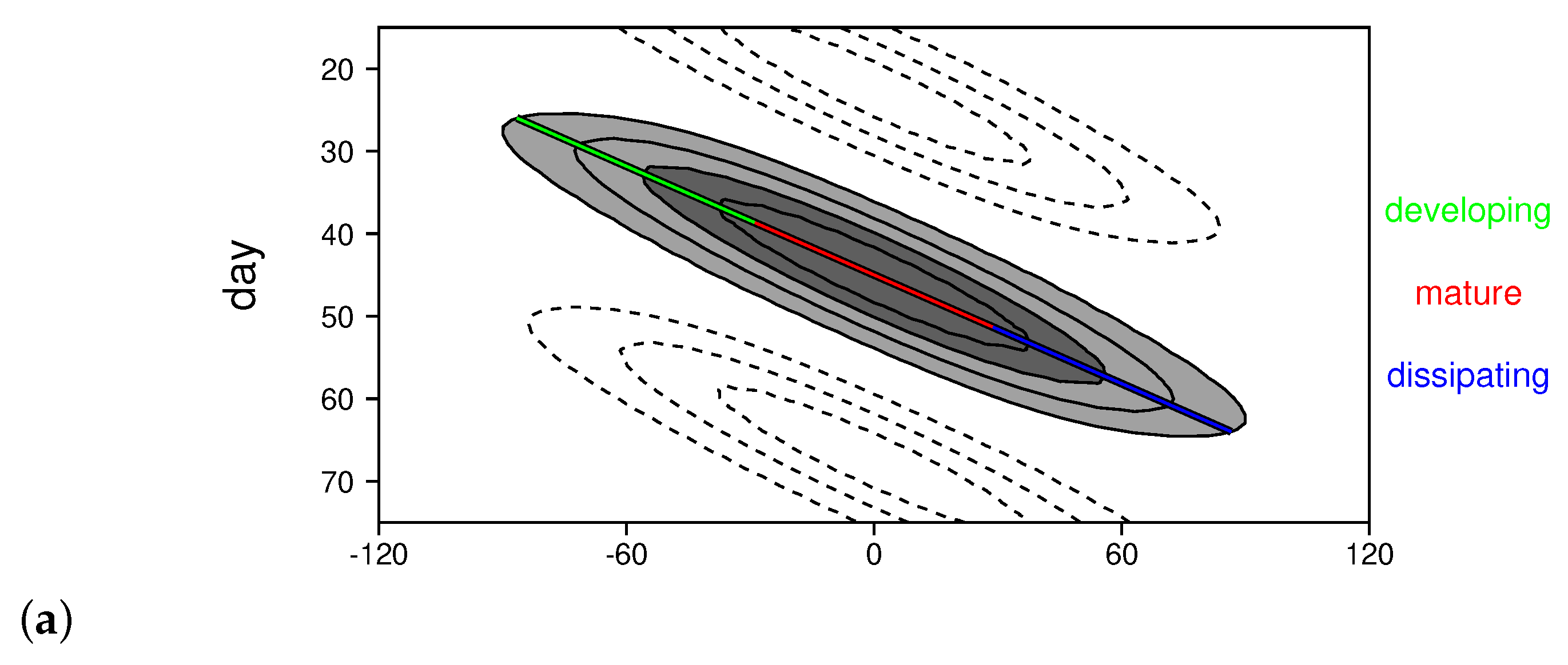
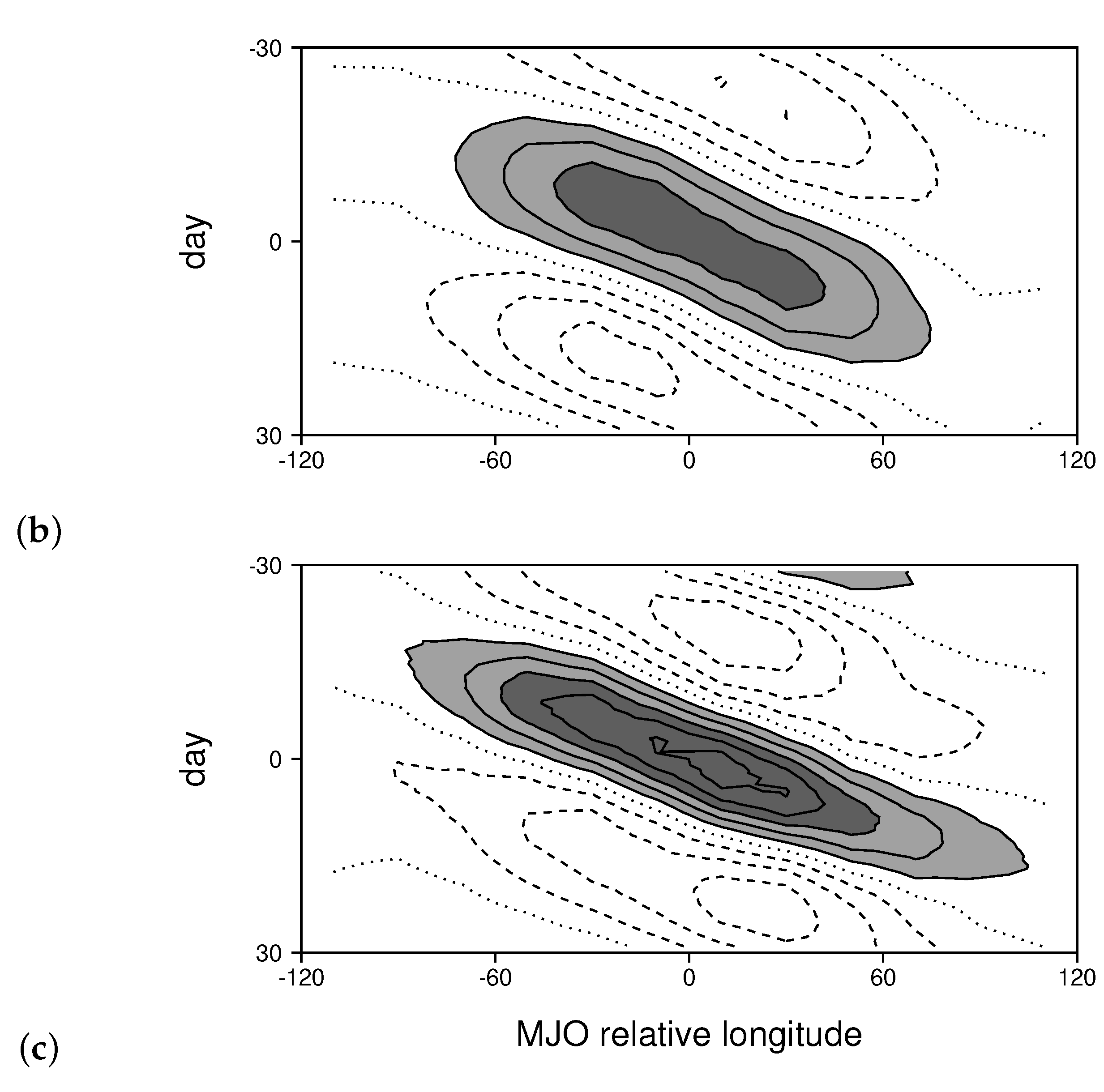
(a) Time longitude series of prescribed mid-level heating for the linear simulation. The contour interval is 0.2 K/day, with values greater that 0.1 K/day shaded light gray and values greater than 0.2 K/day shaded dark gray. Note that this does not include the wave induced heating so the total heating is much stronger. (b,c) Time longitude series of perturbation rainfall for the observed and simulated composite MJOs, respectively. The contour interval is 1 mm/day and values greater than 1 (3) mm/day are shaded light (dark) gray.
Figure 6.
(a) Time longitude series of prescribed mid-level heating for the linear simulation. The contour interval is 0.2 K/day, with values greater that 0.1 K/day shaded light gray and values greater than 0.2 K/day shaded dark gray. Note that this does not include the wave induced heating so the total heating is much stronger. (b,c) Time longitude series of perturbation rainfall for the observed and simulated composite MJOs, respectively. The contour interval is 1 mm/day and values greater than 1 (3) mm/day are shaded light (dark) gray.


Figure 7.
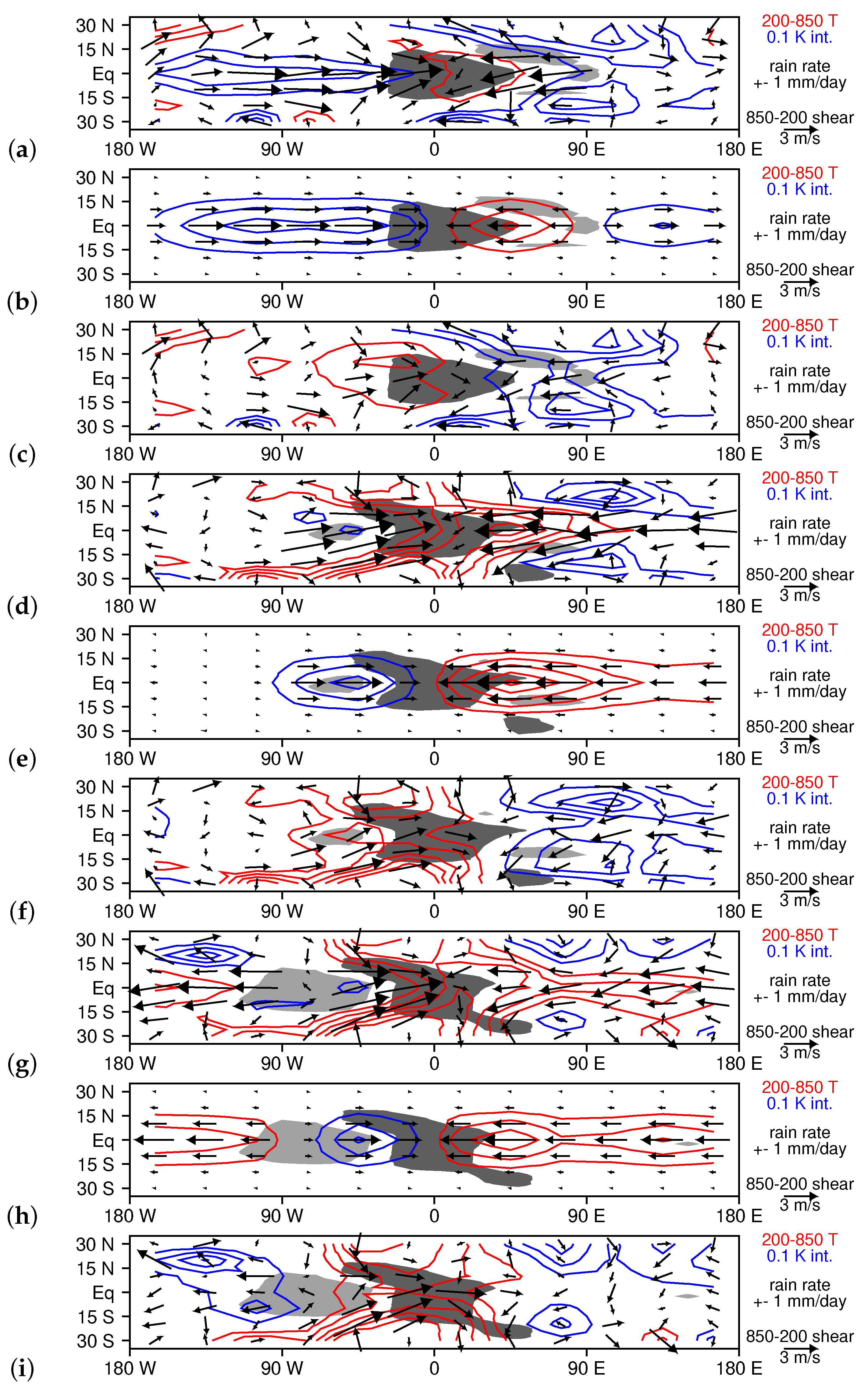
Mean tropospheric temperature (0.1 K contour interval, red for positive and blue for negative) and the difference between 850 hPa and 200 hPa horizontal flow (vectors) for the (a–c) developing, (d–f) mature, and (g–i) dissipating stages of the moving heating. Panels (a,d,g) show the total temperature and flow fields, panels (b,e,h) show the Kelvin wave component, and panels (c,f,i) show the Rossby component (total minus Kelvin wave).
Figure 7.
Mean tropospheric temperature (0.1 K contour interval, red for positive and blue for negative) and the difference between 850 hPa and 200 hPa horizontal flow (vectors) for the (a–c) developing, (d–f) mature, and (g–i) dissipating stages of the moving heating. Panels (a,d,g) show the total temperature and flow fields, panels (b,e,h) show the Kelvin wave component, and panels (c,f,i) show the Rossby component (total minus Kelvin wave).

Figure 8.
Mean tropospheric temperature (0.1 K contour interval, red for positive and blue for negative) and the difference between 850 hPa and 200 hPa horizontal flow (vectors) for the (a–c) developing, (d–f) mature, and (g–i) dissipating stages of the observed MJO (adapted from Reference [25]). Panels (a,d,g) show the total temperature and flow fields, panels (b,e,h) show the Kelvin wave component, and panels (c,f,i) show the Rossby component (total minus Kelvin wave).

Figure 9.
Mean tropospheric temperature (0.1 K contour interval, red for positive and blue for negative) and the difference between 850 hPa and 200 hPa horizontal flow (vectors) for the (a–c) developing, (d–f) mature, and (g–i) dissipating stages of the LAM MJO. Panels (a,d,g) show the total temperature and flow fields, panels (b,e,h) show the Kelvin wave component, and panels (c,f,i) show the Rossby component (total minus Kelvin wave).

Figure 10.
Vertical structure along the equator for the linear simulation with a moving heating for (a) developing, (b) mature, and (c) dissipating stages of the heating, respectively. Temperature is contoured with a 0.2 C interval, and vectors indicate horizontal and vertical wind flow. Dark shading indicates heating greater than 0.1 C/day, and light shading indicates cooling less than C/day.

Figure 11.
Vertical structure along the equator for the observed composite MJO for (a) developing, (b) mature, and (c) dissipating stages of the heating, respectively (adapted from Reference [25]). Temperature is contoured with a 0.2 C interval, and vectors indicate horizontal wind flow. Green (gray) shading indicates moisture perturbations greater than 0.1 (less than ) g/kg.

Figure 12.
Vertical structure along the equator for the composite LAM MJO for (a) developing, (b) mature, and (c) dissipating stages of the heating, respectively. Temperature is contoured with a 0.2 C interval, and vectors indicate horizontal wind flow. Green (gray) shading indicates moisture perturbations greater than 0.1 (less than ) g/kg.

Figure 13.
Vertical structure along the equator for the linear simulation with a moving elevated heating for (a) developing, (b) mature, and (c) dissipating stages of the heating, respectively. Temperature is contoured with a 0.2 C interval, and vectors indicate horizontal and vertical wind flow. Dark shading indicates heating greater than 0.1 C/day, and light shading indicates cooling less than C/day.

Publisher’s Note: MDPI stays neutral with regard to jurisdictional claims in published maps and institutional affiliations. |
© 2020 by the author. Licensee MDPI, Basel, Switzerland. This article is an open access article distributed under the terms and conditions of the Creative Commons Attribution (CC BY) license (http://creativecommons.org/licenses/by/4.0/).
Share and Cite
MDPI and ACS Style
Haertel, P. Kelvin/Rossby Wave Partition of Madden-Julian Oscillation Circulations. Climate 2021, 9, 2. https://0-doi-org.brum.beds.ac.uk/10.3390/cli9010002
AMA Style
Haertel P. Kelvin/Rossby Wave Partition of Madden-Julian Oscillation Circulations. Climate. 2021; 9(1):2. https://0-doi-org.brum.beds.ac.uk/10.3390/cli9010002
Chicago/Turabian StyleHaertel, Patrick. 2021. "Kelvin/Rossby Wave Partition of Madden-Julian Oscillation Circulations" Climate 9, no. 1: 2. https://0-doi-org.brum.beds.ac.uk/10.3390/cli9010002
Note that from the first issue of 2016, this journal uses article numbers instead of page numbers. See further details here.