
The Multiscale Dynamics of the 29 June 2012 Super Derecho


1
Atmospheric Sciences P.h.D. Program, University of Nevada, Reno, NV 89557, USA
2
McGinley & Associates, Inc., a Universal Engineering Sciences Company, Reno, NV 89511, USA
3
Applied Aviation Sciences Department, College of Aviation, Prescott Campus, Embry-Riddle Aeronautical University, Prescott, AZ 86301, USA
*
Author to whom correspondence should be addressed.
Climate 2021, 9(11), 155; https://0-doi-org.brum.beds.ac.uk/10.3390/cli9110155
Submission received: 4 September 2021
/
Revised: 15 October 2021
/
Accepted: 19 October 2021
/
Published: 22 October 2021
(This article belongs to the Special Issue Extreme Weather Events)
Abstract
:The 29–30 June 2012 “super” derecho was, up until the 10 August 2020 “Iowa Derecho”, the most prolific derecho of modern times. While many of the synoptic-scale precursors to derecho events are understood, the multi-scale dynamics which likely distinguish derecho-producing events versus non-derecho events remain much more elusive. Using both observations and high-resolution WRF-ARW simulations, the sequence of adjustments that ultimately set up the pre-29 June derecho environment are examined. Planetary scale Rossby wave breaking occurred almost exactly two weeks before the super derecho on 15–16 June 2012 resulting in the development and intensification of a strong high-pressure system and mixed layer over the complex terrain of the western United States. A week after the initial Rossby wave break (~23 June), daily record-breaking temperatures began to dominate much of the central U.S. as the mixed layer/high pressure continued to strengthen. A second Rossby wave break on 26 June was crucial for detaching the mixed layer from the western U.S. elevated plateau, creating an elevated mixed layer that was rapidly deformed and propagated downstream to set up the derecho environment between 27–29 June. On 28 June, flow imbalance at the elevated mixed layer front resulted in highly ageostrophic circulations in the mid-levels, generating an along-stream mid-level jetlet which ultimately moved the elevated mixed layer and associated mesoscale front downstream across the Midwest and Mid-Atlantic. On the morning of 29 June, a well-defined corridor of both potential static instability and lowered inertial stability was set up across the Midwest and Mid-Atlantic states. This along with strong capping, a divergent polar jet entrance region to the north, and the highly imbalanced mid-level jetlet set the stage for this prolific severe convective event.
1. Introduction
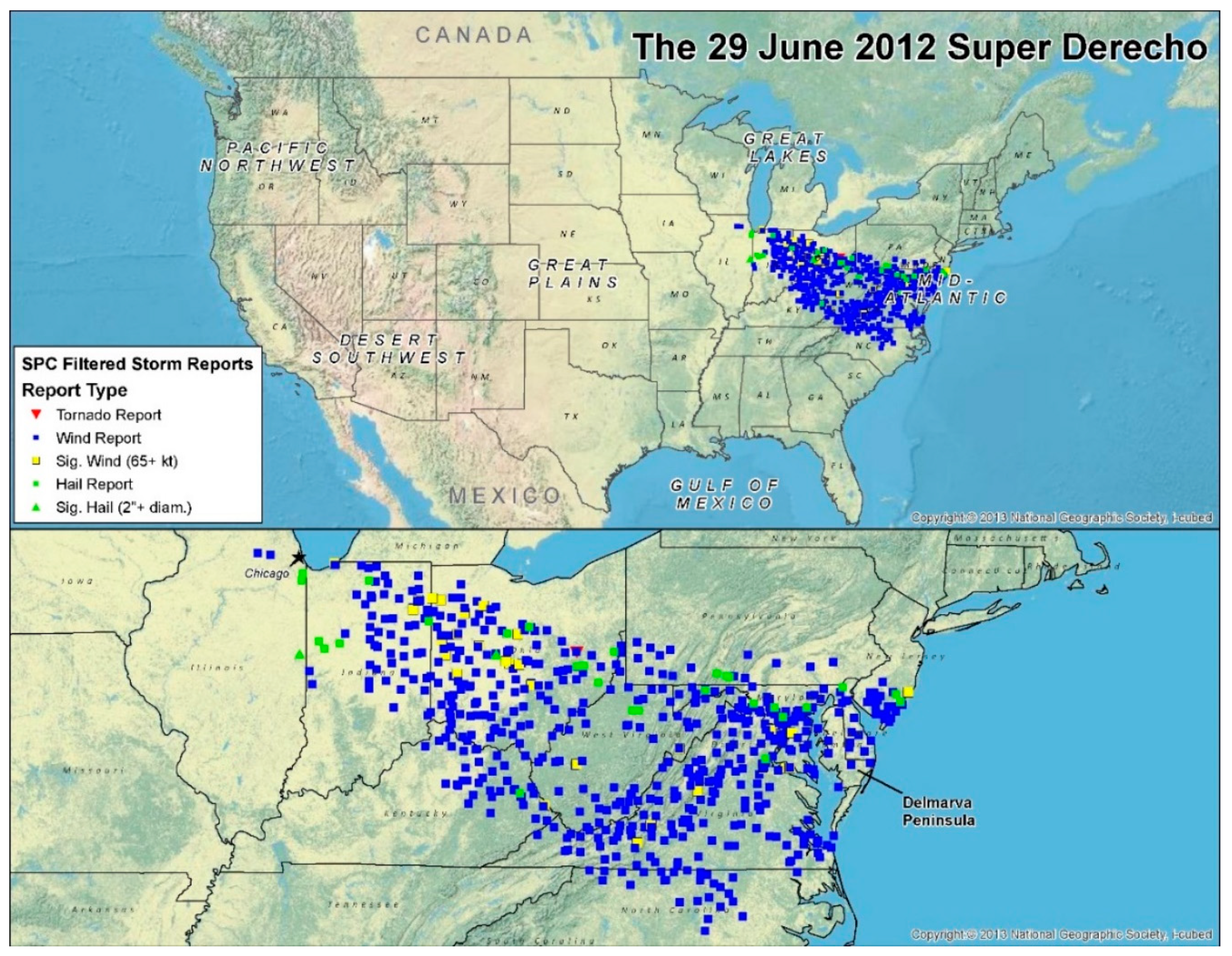
The 29–30 June 2012 “super” derecho, or the 2012 “ring of fire” derecho (Figure 1), traveled over 600 miles, resulting in nearly 675 (filtered) severe wind reports [1], at least USD 2.9 billion in insured damage, and 22 direct fatalities, all within a twelve-hour period [2]. In the weeks following the storm, the heatwave which preceded the derecho continued across the affected region resulting in an additional 34 heat-related deaths as an indirect result of the general circulation that organized the storm. The 29–30 June super derecho was perhaps the most prolific derecho event in contemporary times up until the recent 10 August 2020 “Iowa derecho”, which, much like the 29–30 June 2012 super derecho, was not well forecast by numerical models in the days and even hours leading up to the event.
Early on 29 June 2012, a decaying mesoscale convective vortex (MCV) and its associated cold pool was located over the Dakotas, and by 1300 UTC this cold pool had triggered a cluster of elevated convection over South Dakota [3]. These storms, though expected to intensify [4], ended up dissipating quickly, and a new cluster of elevated convection took off further east along the front caused by the elevated mixed layer (EML) near the Iowa/Illinois border around 1400 UTC. These storms continued eastward along the EML front (EMLF; i.e., the leading edge of the EML), finally orienting north-south around 1700 UTC as the storm complex passed to the south of Lake Michigan and associated cool air.
As this developing mesoscale convective system (MCS) crossed into northwest Indiana, additional convection was triggered across west-central Indiana that then “merged” with the initial MCS between 1800 and 1900 UTC. This merger appears to be a key event in the development of the 29 June 2012 super derecho because from this point on, the MCS strengthened very rapidly into a highly organized and intense bow echo. It was also around this time that the maximum recorded wind gust for the system occurred, with an observed gust of 91 mph in Fort Wayne, Indiana, at 1854 UTC. From there, the derecho continued to grow upscale as it propagated east-southeast towards the Atlantic Coast. By 0500 UTC on 30 June 2012, just twelve hours after initial MCS development, the system exited the contiguous United States (CONUS) off the Delmarva Peninsula coast while still causing severe wind damage and triggering several special marine warnings.
The current body of literature that exists on derechos is largely dominated by synoptic climatologies and ingredients-based, synoptic-scale conceptual models [5,6,7,8,9,10,11,12], as well as detailed case studies of specific events [3,13,14,15,16,17,18,19,20,21], but little work has been done regarding the multiscale links and nonlinear dynamic processes that precede, generate, and maintain the intense and unique mode of convection that is the derecho. Documentation of derechos dates to at least the late 1800s [22] and they are a well-understood phenomenon on their own, but the environments in which derechos form are largely misunderstood which makes derecho forecasting challenging. A more detailed derecho literature review and description of a warm-season derecho setup are presented in the first author’s master’s thesis, from which this work is derived [23]. Even though the environment on 29 June 2012 was, by all standards, a classic warm-season derecho setup, model inconsistencies contributed to forecaster uncertainty and only isolated severe weather across the subsequently affected region was anticipated for 29 June just one day before the event [1,2,24].
The multiscale analysis of the 29 June 2012 derecho presented herein utilizes both observations and mesoscale numerical simulations to diagnose the links among the polar jet, elevated mixed layer front, scale-contracted ridge, mid-level mesoscale jetlet(s), and cold pool, adding to the overall understanding of derecho development and maintenance in hopes of ultimately improving operational, warm-season derecho forecasting. The analysis herein utilizes isobaric fields alongside isentropic fields for a more complete diagnosis of these processes, particularly with regards to the EML and ageostrophic mid-level jetlet development. Although only one case study, insights from this analysis may improve the linkages among the numerous ingredients-based synoptic regimes presented throughout the literature for improved derecho forecasting.
2. Materials and Methods
Two different approaches are taken in this analysis of the 29 June 2012 super derecho. First, the observational analysis of the event was conducted using available surface and upper air data, mesoscale analyses, remotely sensed satellite, and radar data, etc. The upper air data, vertical soundings, and reanalyses were retrieved from the SPC (Storm Prediction Center) Severe Weather Events Archive [25] and the University of Wyoming [26]. Surface data was also gathered from the SPC Severe Weather Events Archive. Radar and satellite imagery of the event was collected from the SPC archive [25], NOAA Environmental Visualization Laboratory [27], Unisys Weather (website no longer available), UCAR’s weather data archive [28], and the SPC’s case page for this storm [1,25,29]. High-temperature records from the National Climatic Data Center (NCDC) daily weather records data tool [30] were also utilized. Additional details and information from various news articles, meteorological blog posts, and official government reports and memorandums on the event were reviewed.
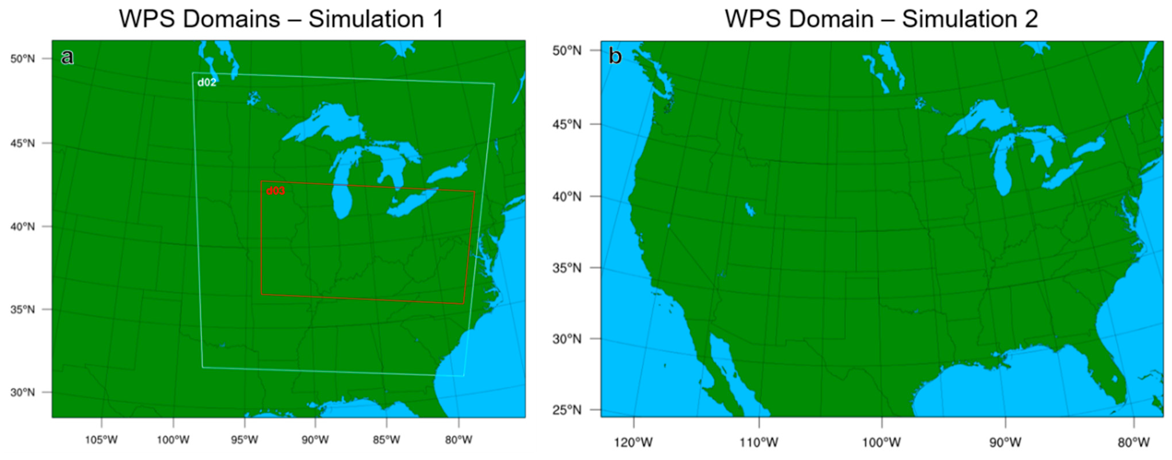
The second approach for this analysis was to simulate the 29 June event and precursor environment using a high-resolution numerical model with 18 km, 6 km, and 2 km model domains. WRF-ARW version 3.7.1 [31] was employed for this purpose, and two simulations were run: a one-way nested, three-domain simulation (Simulation 1) run over the areas of interest, and a larger, one domain simulation (Simulation 2) covering the entire CONUS. The full details of each of these simulations are summarized in Table 1, and the model domains are displayed in Figure 2.
Simulation 1 is one-way nested with three domains at 18 km, 6 km, and 2 km horizontal grid spacing. Simulation 2 is a single domain simulation at 18 km grid spacing to capture a larger portion of the CONUS for synoptic analysis of the event and the multiday precursor conditions. Both simulations were initialized using the National Center for Environmental Prediction (NCEP) Final Global Analysis (FNL) on a 1° × 1° grid with 26 vertical pressure levels. The NCEP FNL data is available at 6-hour intervals daily from the NCAR/UCAR Computational and Information Systems Lab Research Data Archive [32].
All of the WRF-ARW simulations run for this study have 28 vertical levels and use the Thompson microphysics scheme [33] and Mellor–Yamada–Janjic PBL (planetary boundary layer) scheme [34,35] for consistency with the Weisman et al. [16] 3 km simulation of the 8 May 2009 super derecho which utilized the same. Convection is explicitly resolved in the 2 km model domain, and the Grell–Freitas cumulus scheme [36] is used in the 18 km and 6 km simulation domains. The Simulation 1 18 km and 6 km simulations were run from 1200 UTC 24 June to 0600 UTC 30 June 2012 (120 h), and the 2 km simulation was run from 0600 UTC 29 June to 0600 UTC 30 June 2012 (12 h, allowing for six hours of spin-up plus five additional hours prior to derecho initiation which occurred around 1700 UTC). Simulation 2 was run from 1200 UTC 24 June to 1200 UTC 29 June 2012.

Table 1.
Summary of WRF-ARW 3.7.1 [31] Model options used in Simulations 1 and 2.
Table 1.
Summary of WRF-ARW 3.7.1 [31] Model options used in Simulations 1 and 2.
| WRF Model Options | Domain 1 (Simulations 1 and 2) | Domain 2 | Domain 3 |
|---|---|---|---|
| Horizontal resolution | Simulation 1: 18 km (116 × 94) Simulation 2: 18 km (259 × 177) | 6 km (265 × 175) | 2 km (643 × 412) |
| Vertical resolution | 28 levels; top 100 hPa | 28 levels; top 100 hPa | 28 levels; top 100 hPa |
| Surface layer option | Eta Similarity Scheme [34,37,38,39] | Eta Similarity Scheme [34,37,38,39] | Eta Similarity Scheme [34,37,38,39] |
| PBL physics option | Mellor–Yamada–Janjic Scheme [34,35] | Mellor–Yamada–Janjic Scheme [34,35] | Mellor–Yamada–Janjic Scheme [34,35] |
| Cumulus parameterization option | Grell–Freitas Ensemble Scheme [36] | Grell–Freitas Ensemble Scheme [36] | N/A |
| Microphysics option | Thompson Scheme [33] | Thompson Scheme [33] | Thompson Scheme [33] |
| Shortwave radiation option | Dudhia Shortwave Scheme [40] | Dudhia Shortwave Scheme [40] | Dudhia Shortwave Scheme [40] |
| Longwave radiation option | RRTM Longwave Scheme [41] | RRTM Longwave Scheme [41] | RRTM Longwave Scheme [41] |
| Land surface option | Unified Noah Land Surface Model [42] | Unified Noah Land Surface Model [42] | Unified Noah Land Surface Model [42] |
Observational data was used to verify the accuracy of the simulation prior to conducting a simulation-based diagnosis of the event. The results of both the model verification and the simulations are presented in Section 3.2. Given the relative accuracy with which the model was able to simulate the 29 June event, both the observational and model analyses presented herein proved extremely useful for diagnosing the mechanisms which lead to such an intense derecho.
3. Results
3.1. Observational Analysis
3.1.1. 15–26 June: Synoptic Scale Overview
Consistent with Cordeira et al. [43], Rossby wave train amplification occurred over the northeastern Pacific/western U.S. almost two weeks ahead of the super derecho with subsequent Rossby/Planetary Wave Breaking (RWB/PWB) occurring seven days prior to the development of an intense EML over the southcentral and southwestern U.S. On 15–16 June, an RWB occurred over the U.S. Pacific Northwest and extreme southwestern U.S. 22–23 June 2012 marked the beginning of the June–July 2012 heat-wave which caused fires across the central U.S., record-breaking high temperatures across much of the central and eastern portions of the country, the 29 June super derecho, additional strong convective outbreaks (including a derecho series from 29 June through 4 August), and numerous fatalities as both a direct and indirect result of the heat.
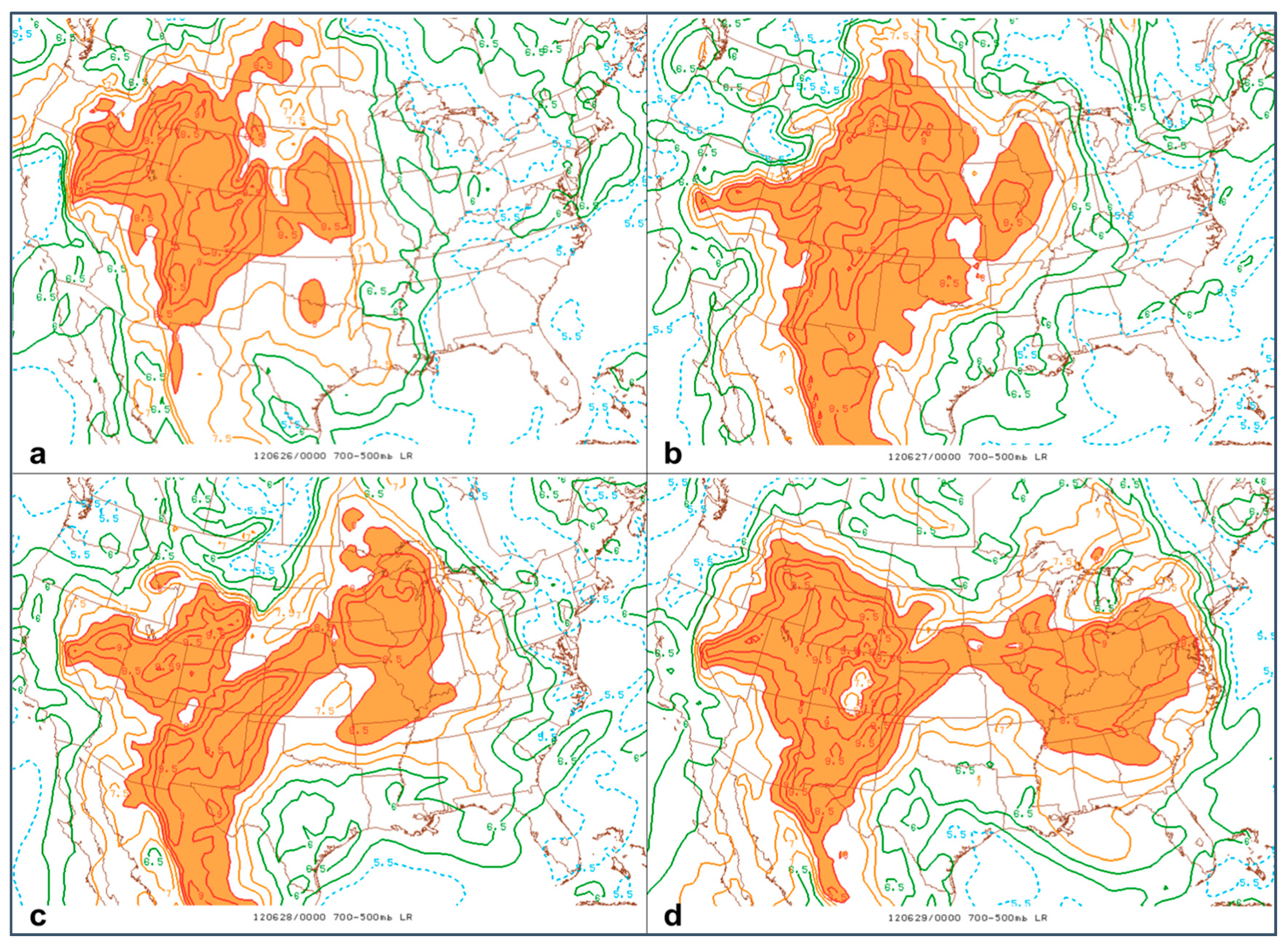
From 23–26 June, the EML continued to expand in scale and intensify. National Weather Service (NWS) radiosonde upper air soundings (not pictured) and SPC experimental RAP (WRF-Rapid Refresh) analysis 700–500 hPa mid-level lapse rates (00Z 26 June mid-level lapse rates and EML location shown in Figure 3a) were employed to track the deformation and advection of the EML downstream from the south/central Great Plains to the Midwest and Mid-Atlantic regions (Figure 3a–d). Although a few initial surges of the EML occurred prior to June 27, the relative weakness of these EML perturbations and associated EMLFs in part prevented derecho-producing convection from occurring in the days leading up to the actual 29 June derecho.
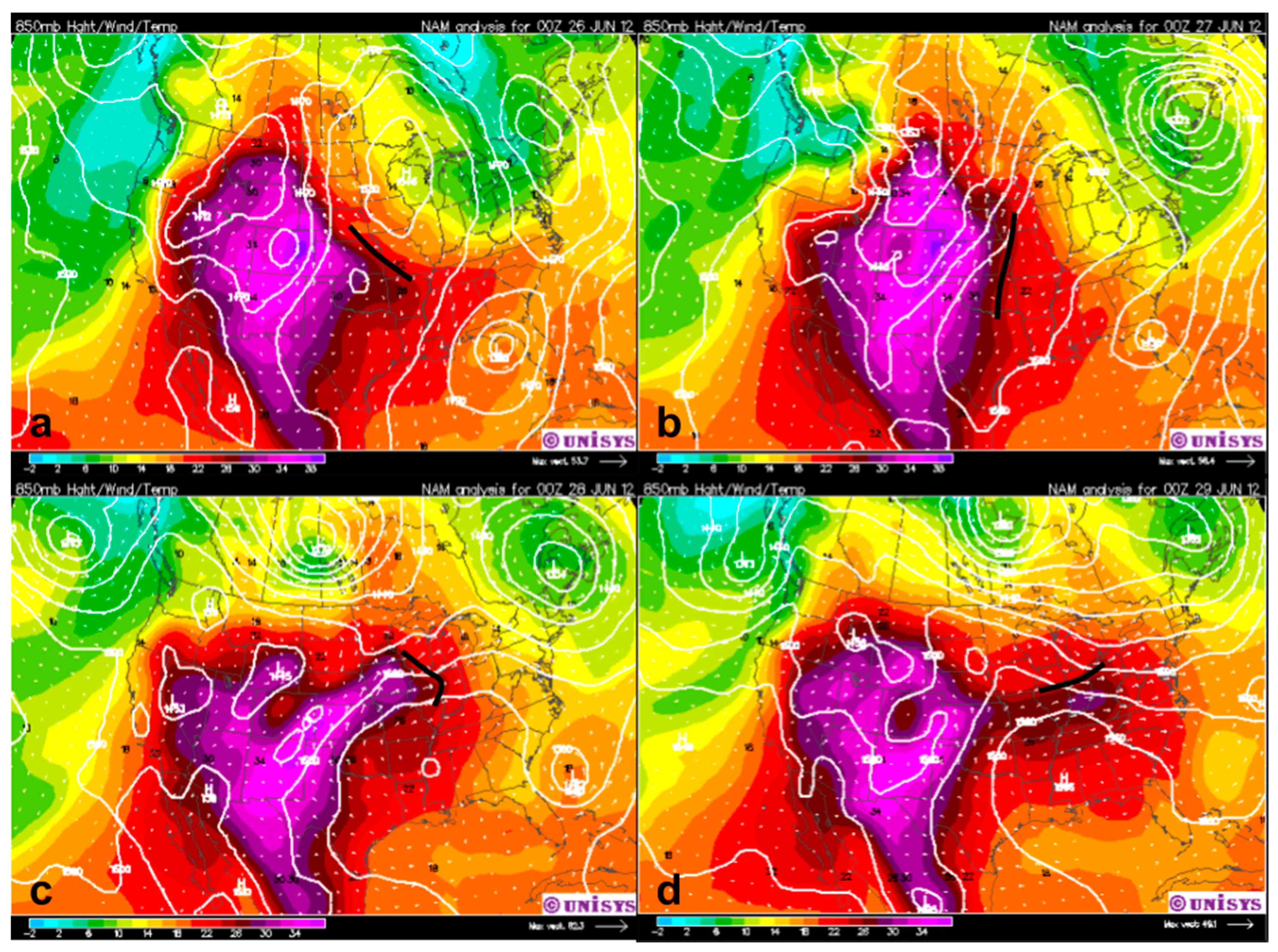
A second RWB took place between 12Z 25 June and 12Z 26 June 2012, resulting in the movement of the polar jet streak and low-pressure systems east-northeastward over southern Canada which triggered the detachment and advection of the EML downstream (Figure 4).
3.1.2. 27–29 June: Heatwave and Precursor Bow Echoes
On 0000 UTC 27 June, post RWB, the low-pressure system off the Pacific Northwest began moving inland across southern Canada and the U.S. interior northwest. Movement of the associated polar jet streak around the ridge juxtaposed the divergent right entrance region of the jet streak and the outer edges of the EML, inducing the lifting of air up and out of the mixed layer while deforming and advecting the core of the hot air downstream. The movement of this core of hot air downstream is evident in the progression of mid-level relatively unstable lapse rates from 26 June to 29 June in Figure 3 (orange color fill indicating lapse rates of ≥8 °C/km). By 1200 UTC 27 June low pressure was located over the Canadian provinces of Alberta and Saskatchewan, aiding in the propagation of the dome of high pressure poleward and eastward as the low continued to push east/northeast.
During the week leading up to the 29 June 2012 derecho, over 164 all-time high-temperature records were broken in the U.S. An additional 2174 daily and monthly temperature records were also tied or exceeded during this time for a total of 2338 record high temperatures. A day-by-day breakdown of temperature records from the June/July 2012 heatwave is provided in Table 2. Record-breaking temperatures began across the central and southern Great Plains and spread poleward and westward over the course of the week leading up to the derecho. By 29 June the ridge of high pressure over much of the CONUS began to flatten out as the low-pressure system and jet streak moved over southern Ontario and extreme northern parts of the Great Lakes region, yet hundreds of high-temperature records continued to be broken even after the 29 June 2012 derecho as the EML and coupled high-pressure center remained situated over parts of the Midwest, Tennessee River Valley, and Mid-Atlantic regions.
On 28 June there were a couple of relatively small bowing MCS which generated a non-trivial number of wind reports (75 reports between two bowing segments [44]) prior to the main derecho event the following day. These small bow echoes each formed with initial surges of hot air eastward from the EML ahead of the main surge on 29 June. The first 28 June bow echo initiated just south of Lake Michigan near the Chicago metropolitan area and caused severe wind reports from Chicago into north-central Indiana, and the second bow echo was triggered over extreme northwestern Pennsylvania just downstream of Lake Erie and traveling all the way to the Atlantic Coast of New Jersey. The second bow was particularly impressive, growing upscale quite rapidly in conditions very similar to those present in the 29 June super derecho, but less intense and on a smaller scale.
3.1.3. 29–30 June: The “Super Derecho”
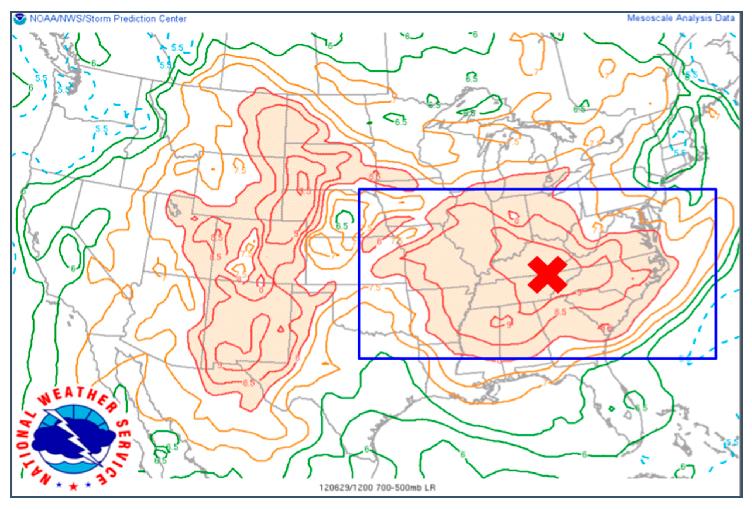
At 1200 UTC on 29 June (Figure 5) the RAP analysis mid-level lapse rates were indicative of the northern edge of the EML (with mid-level lapse rates of ≥8 °C/km) draped across northeastern Iowa southwest into west-central Ohio.
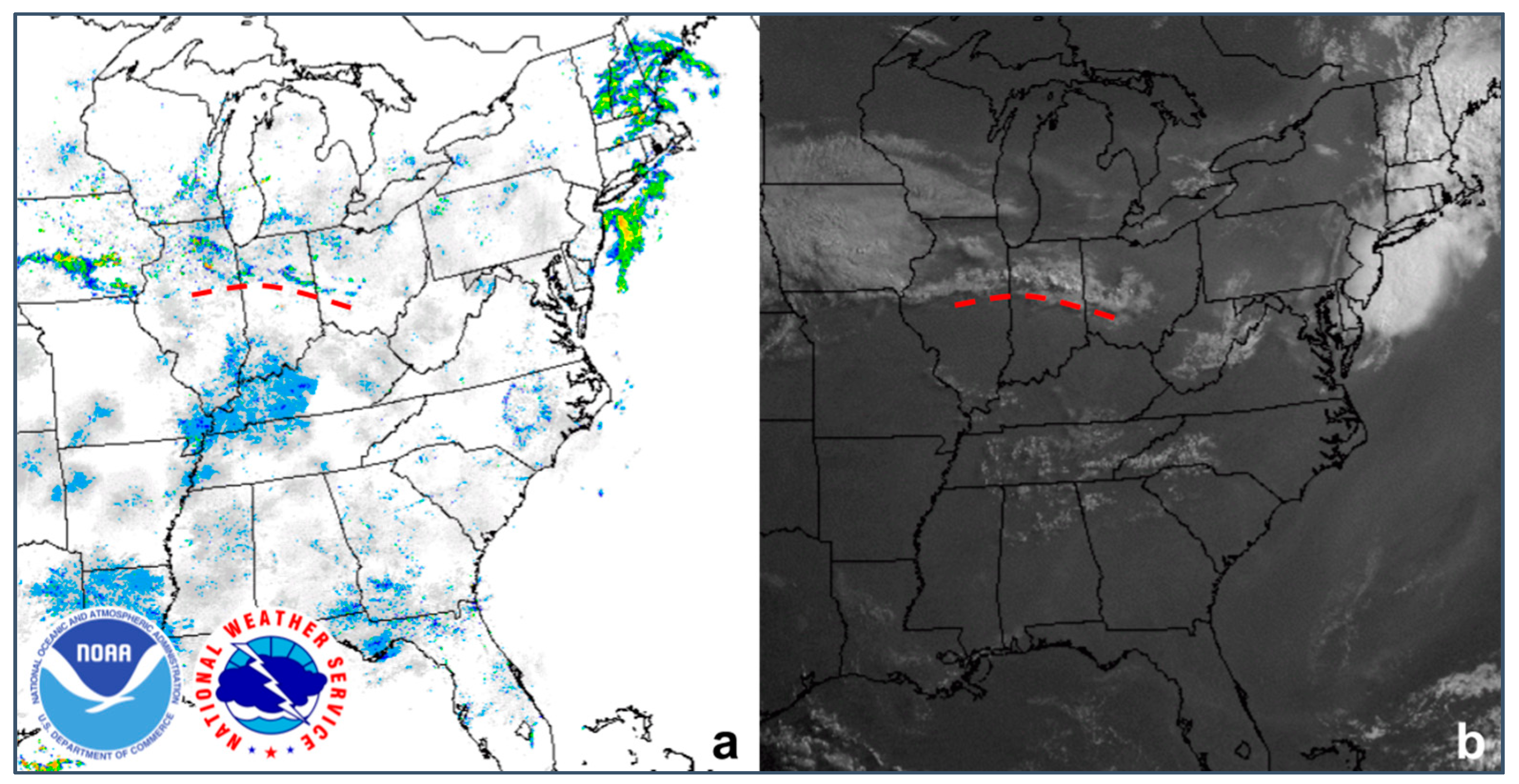
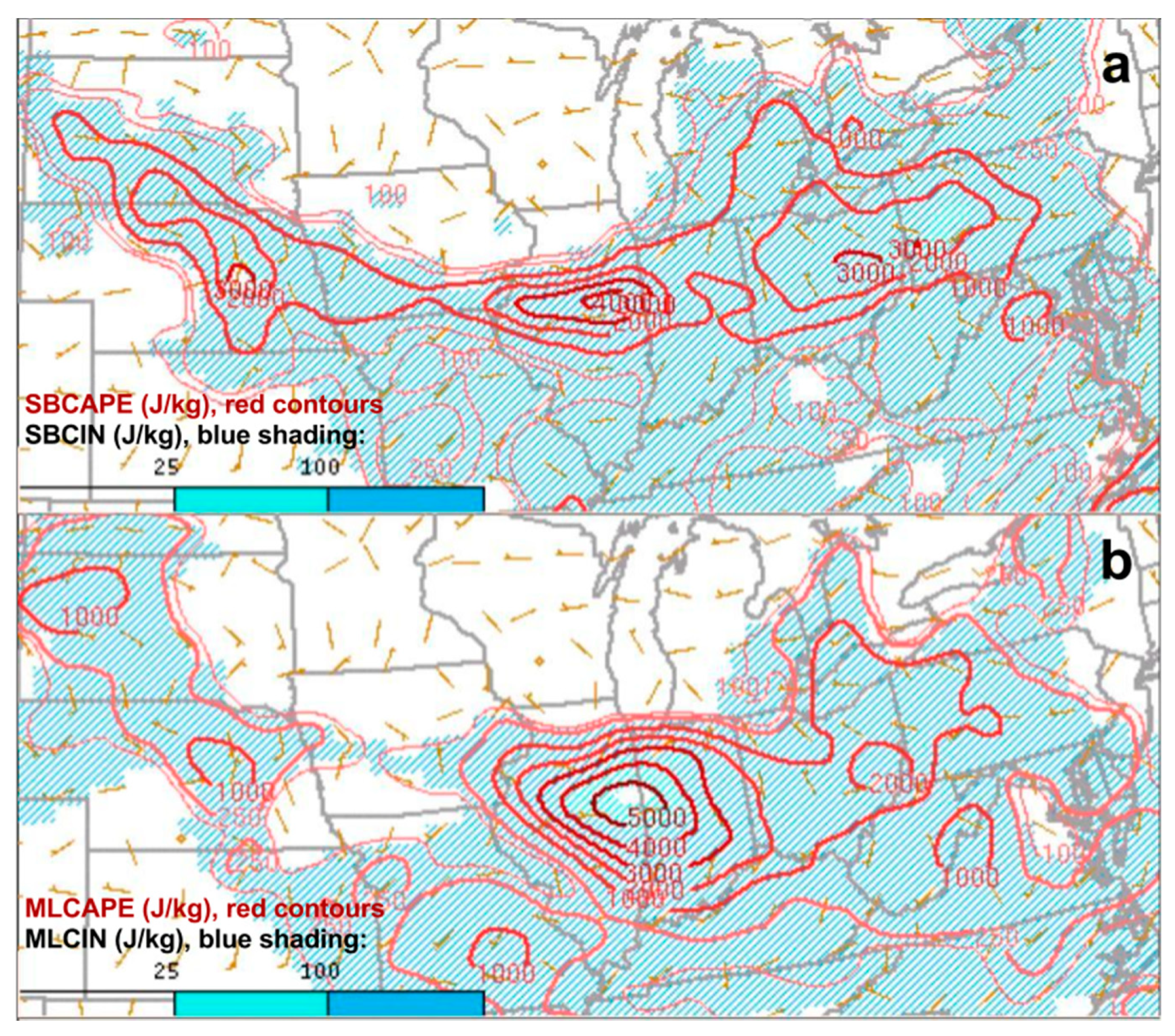
The NOAA SPC 1614 UTC 29 June Day 1 Convective Outlook [25] noted this front to be the “trailing edge” of an occluding surface low over the Canadian provinces of extreme northern Ontario and Quebec. Figure 6 shows the EML boundary on visible satellite imagery as a line of altocumulus castellanus or high-based shallow convection. This same boundary is also apparent on Doppler radar as evidence of the EML overrunning cool, moist air under the divergent polar jet streak right entrance region near the Great Lakes. This process also resulted in a highly stable lid (CIN values of 100+ J/kg, Figure 7) which suppressed deep convection and kept the EML essentially “untouched”, maintaining a corridor of extremely high potential instability.
With high pressure, the EML established across much of the eastern U.S., large-scale subsidence and broad anticyclonic flow were present over regions soon to be impacted by the super derecho. The EMLF on 29 June 2012 was represented on observational surface analyses as a quasi-stationary front across the most poleward extent of the EML (not pictured) and provided a zone of concentrated convergence and uplift along the front.
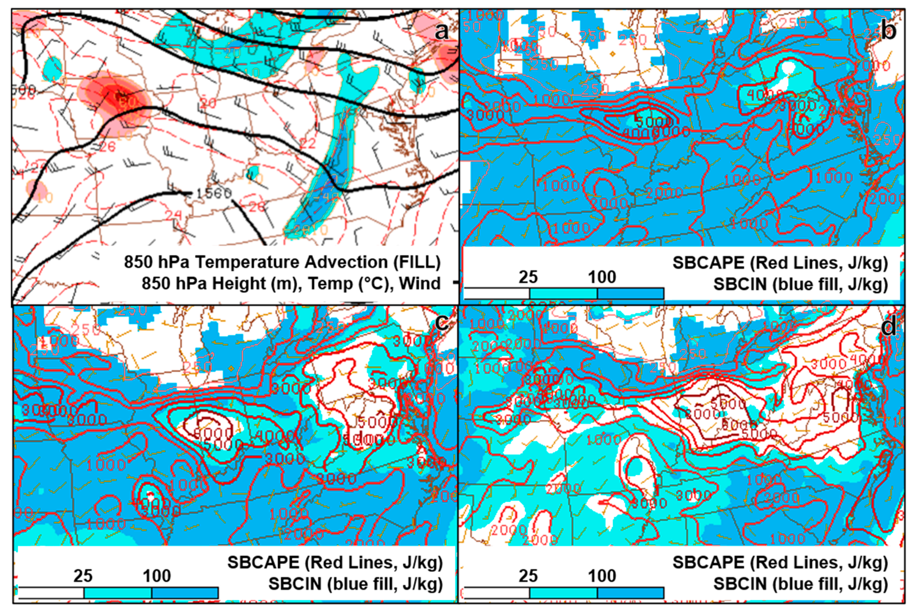
At 1200 UTC a 300 hPa jet streak (70+ knots) was located to the north of the derecho zone extending from central Wisconsin, across Michigan, and equatorward into extreme northeastern Ohio and northwestern Pennsylvania. The 1300 and 1400 UTC 300 hPa RAP analyses in Figure 8 show divergence in the right entrance region of the jet streak, coincident with the surface EMLF, indicating likely surface pressure falls and surface convergence strengthening the EMLF. The presence of this divergent jet streak region also aided in low-level warm air advection (Figure 9a) into the area and advection of the EML further downstream. As the EML continued to be deformed and advected downstream, the strong EML-associated capping layer began to erode within the corridor of highest instability (Figure 9b–d). Cap erosion continued through the afternoon and evening hours until nightfall on 29 June.
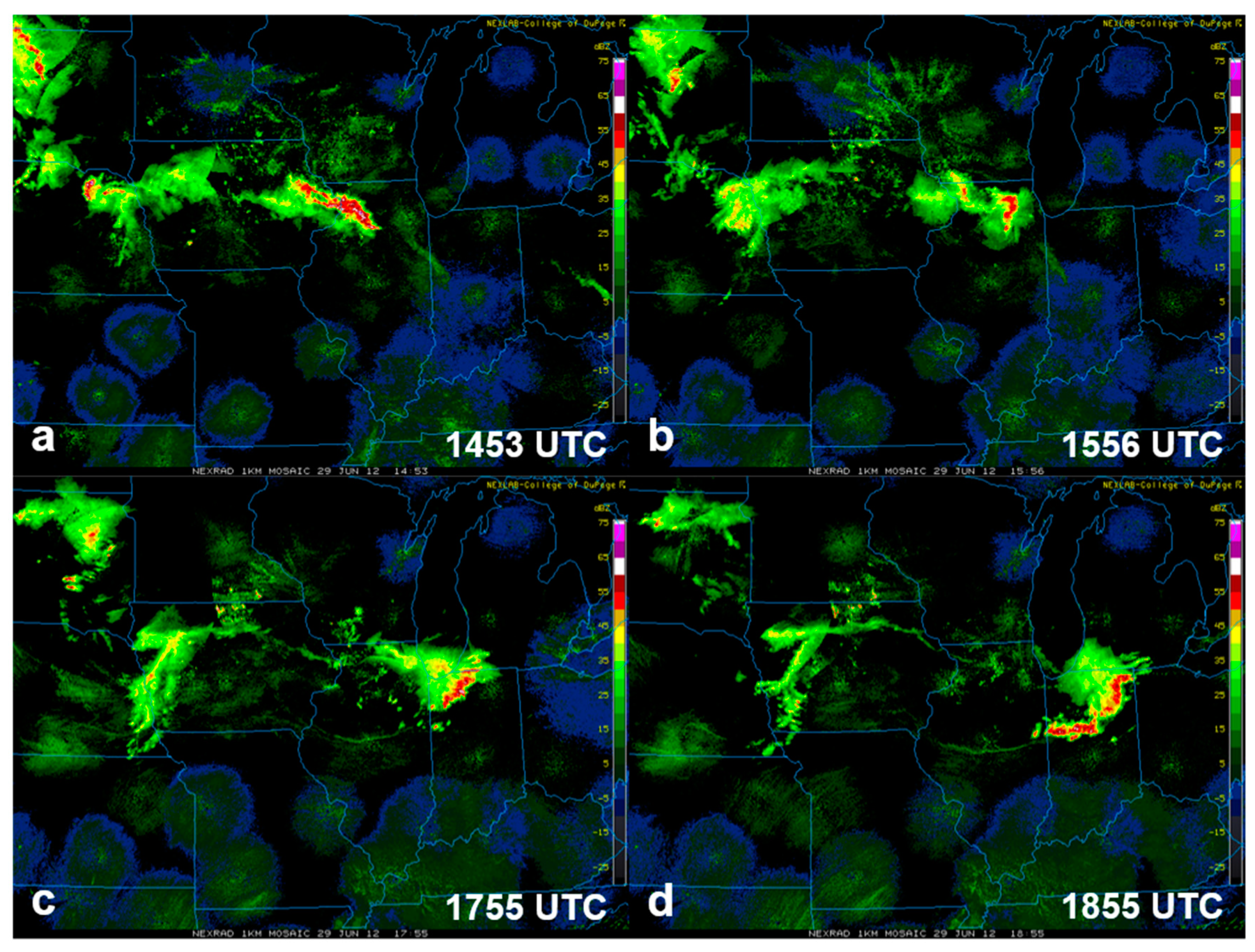
Before 1400 UTC there was little organized convection upstream of the corridor of maximum instability. Between 1400 and 1500 UTC (Figure 10a), a cluster of intense convection developed over extreme east-central Iowa and northern Illinois, with radar reflectivity values surpassing 55 dBz. By 1600 UTC, this convection became more north-south oriented (Figure 10b) just to the west-northwest of the Chicago, Illinois metropolitan area while maintaining intensity. This slightly bowing line of storms began to expand in spatial coverage as it passed the southern tip of Lake Michigan and its associated cold pool [3].
As discussed in Bentley and Logsdon [3], it was by approximately 1800 UTC that this convection became cold pool driven over northwestern Indiana (Figure 10c). By 1830 UTC, the linear MCS began to exhibit strong bowing as it continued to move across northern Indiana. Between 1830 and 1900 UTC (Figure 10d), another cluster of storms developed over portions of west-central Indiana and merged with the bowing MCS by 1900 UTC. It was during the time of this merger that the maximum wind gust report for this derecho event was recorded, with a gust of 91 mph recorded at the Fort Wayne International Airport in northeastern Indiana at 1845 UTC.
While the developing derecho continued to travel along the corridor of extreme instability, displayed on the analyses by a narrow zone of high CAPE values juxtaposed against a region of high DCAPE values (not shown), the storm continued to produce strong downdrafts and severe wind damage all the way to the Mid-Atlantic coast [1,3,13]. These rain-cooled downdrafts continued to reinforce the storm’s intense cold pool [3] which allowed the storm to remain cold pool driven as it continued across the CONUS for the next 10 h until exiting the Mid-Atlantic coast in the early hours of 30 June. Additional anticyclonic outflow aloft also likely enhanced the region of already lowered inertial instability downstream from the derecho, as low inertial stability favors the generation of anticyclonic vorticity [46].
3.2. Model Analysis
3.2.1. Model Performance
To resolve the meso-β/ɣ scale [47] dynamics associated with the 29 June 2012 super derecho the WRF-ARW was utilized as described in Section 2. The 18 km, 6 km, and 2 km WRF-ARW runs were compared against observations of the 29 June derecho as well as the environment in the days leading up to the event. No additional observations (e.g., radar data) were assimilated during model initialization aside from the NCEP FNL reanalysis data. Despite this, the 2 km simulation from 0600 UTC 29 June through 0600 UTC 30 June recreated the super derecho with a high degree of accuracy as can be observed in a comparison of 1800 UTC 29 June through 0400 UTC 30 June 202 observed and WRF-ARW simulated reflectivity (Figure 11). Although the 2 km simulation is spatially biased slightly southwest and temporally biased ~15–30 min too fast (particularly towards the end of the derecho event), the accuracy with which the event was simulated provides a unique opportunity to understand the meso-β/ɣ scale processes involved in generating and maintaining such an intense and long-lived derecho. While the 18 km and 6 km simulations did not resolve the derecho (or any strong, coherent MCS at all), they still provide useful information regarding the larger-scale environment in place before and during the derecho.
3.2.2. 25–28 June: The Precursor Environment
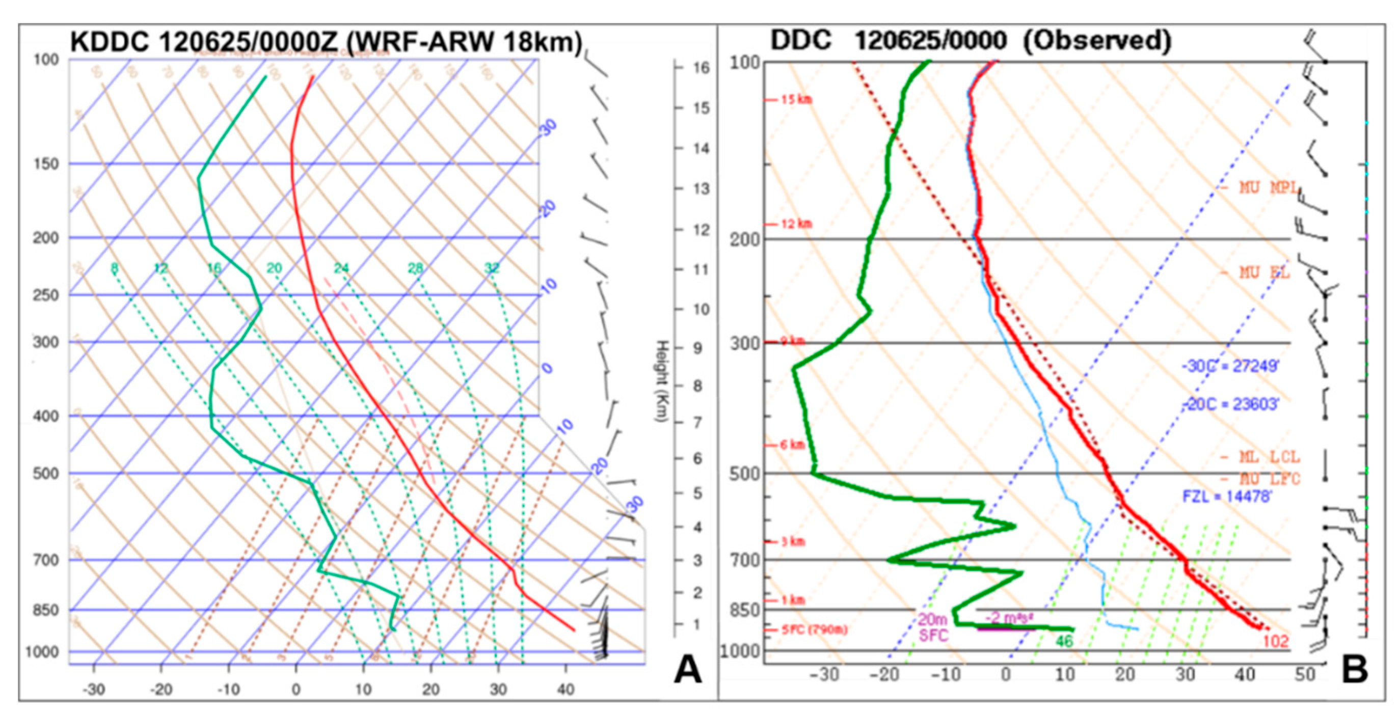
At 0000 UTC 25 June 2012, the core of high pressure and EML was centered over its source region in the U.S. Desert Southwest and Great Basin. A narrower node of well-mixed air and high pressure was also present over eastern Colorado and extreme west-northwest Kansas. Model-simulated vertical soundings (18 km) were compared to observed soundings from Denver (KDNR, Figure 12) and Dodge City (KDDC, Figure 13) and while the soundings do not match exactly, the accuracy with which the 18 km simulation was able to capture the EML environment is encouraging despite the errors. Slight wind errors exist early in the simulation and dew point temperature vertical profiles are smoothed out compared to the observed vertical soundings.
Comparing the 0000 UTC 25 June observational RAP surface analysis with the 18 km WRF-ARW-simulated two-meter temperatures and ten-meter winds (not shown), it is revealed that most major features in the simulation are displaced significantly eastward from the observed surface features. Most notably, Tropical Storm Debby is located well into the eastern Gulf of Mexico in the observational RAP analysis, whereas the WRF-ARW simulation places the system over west-central Florida. Back to the west, the core of hottest temperatures is also located too far eastward in the simulation, surface winds off the southern California coast and Baja Peninsula vary quite a bit, and the hot air does not extend as far northward into Montana.
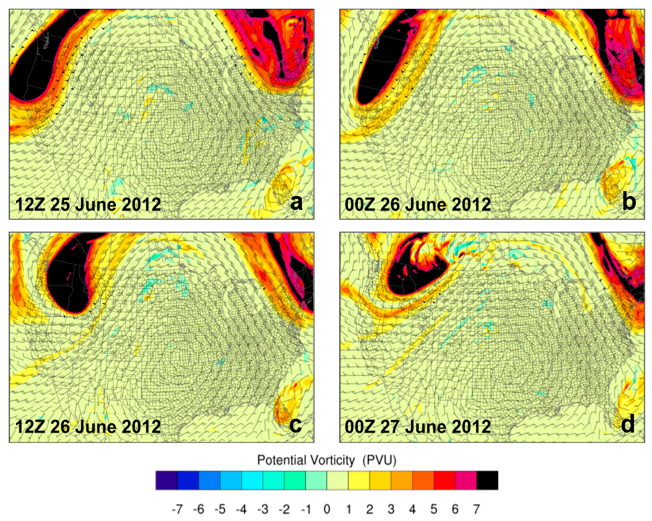
As discussed in Section 3.1.1, planetary wave breaking over the U.S. Pacific Northwest occurred for a second time (the first occurring 15–16 June) ahead of the super derecho event on 26 June 2012. This is seen in the 18 km simulation 320 K, 330 K, and 340 K isentropic potential vorticity fields from 1200 UTC 25 June through 27 June (Figure 14 shows the 330 K isentropic vorticity fields at these times; 320 K and 340 K fields not shown). Anticyclonic wave breaking and overturning of IPV is evident in these fields through a decrease in positive IPV and an increase in negative IPV between 1200 UTC 26 June and 0000 UTC 27 June. Additionally, the wave-breaking process over the northwestern United States is observed in the generation of well-defined positive IPV streamers (elongated maxima or minima of IPV) on both the 330 K and 340 K isentropic surfaces during the same period.
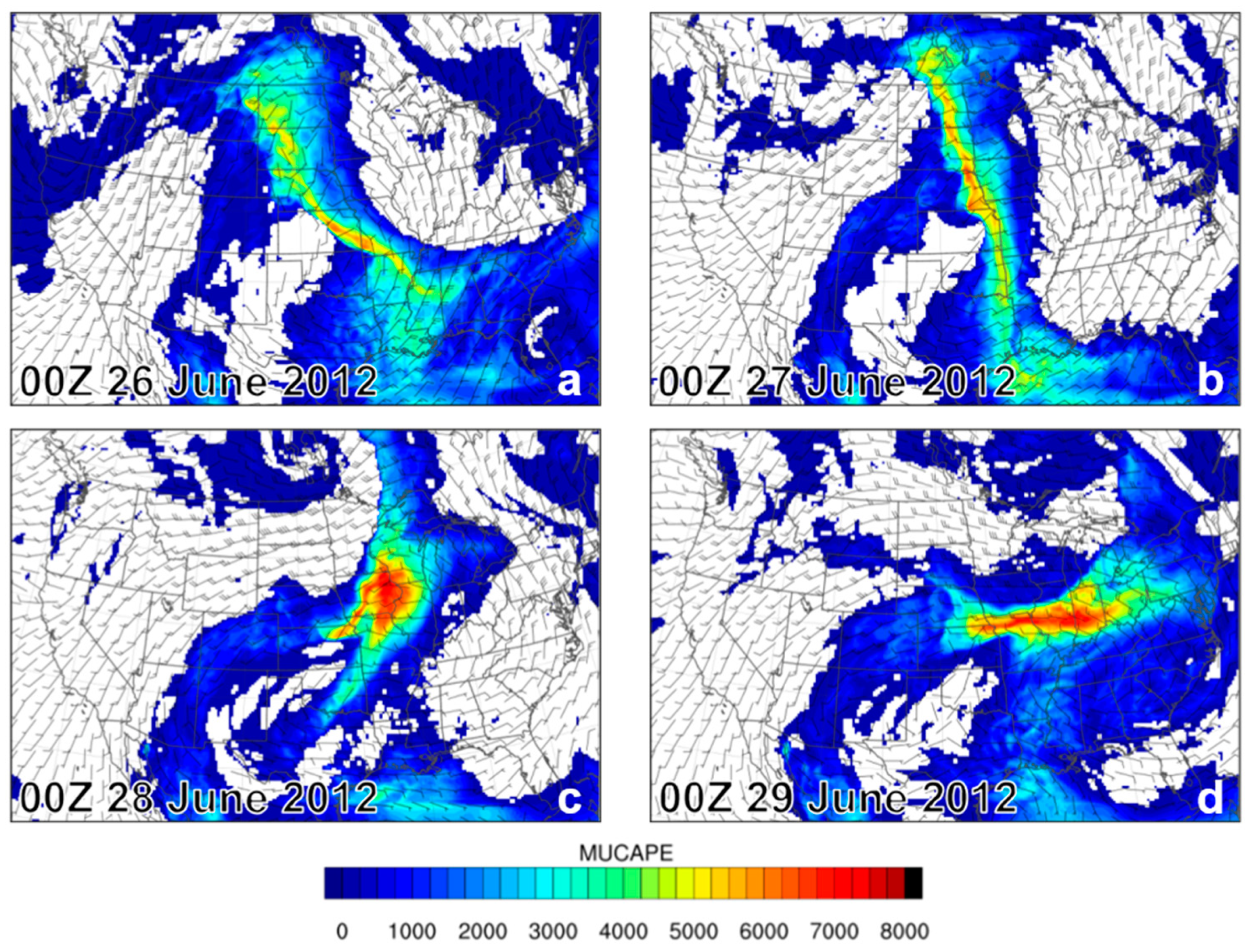
By 27 June 2012, the core of the ridge/mixed layer started to extend north-northeast. This can be seen in the simulated maximum CAPE plots from 0000 UTC 27 June to 0000 28 June in Figure 15. The 0000 UTC 25 June through 0000 UTC 27 June two-meter simulated temperatures, dew points, and ten-meter winds (not shown) also indicate the eastward movement of the mixed layer with the RWB as a portion of the mixed layer was forced north and east by the incoming low-pressure system and associated jet streak over British Columbia and the U.S. Pacific Northwest.
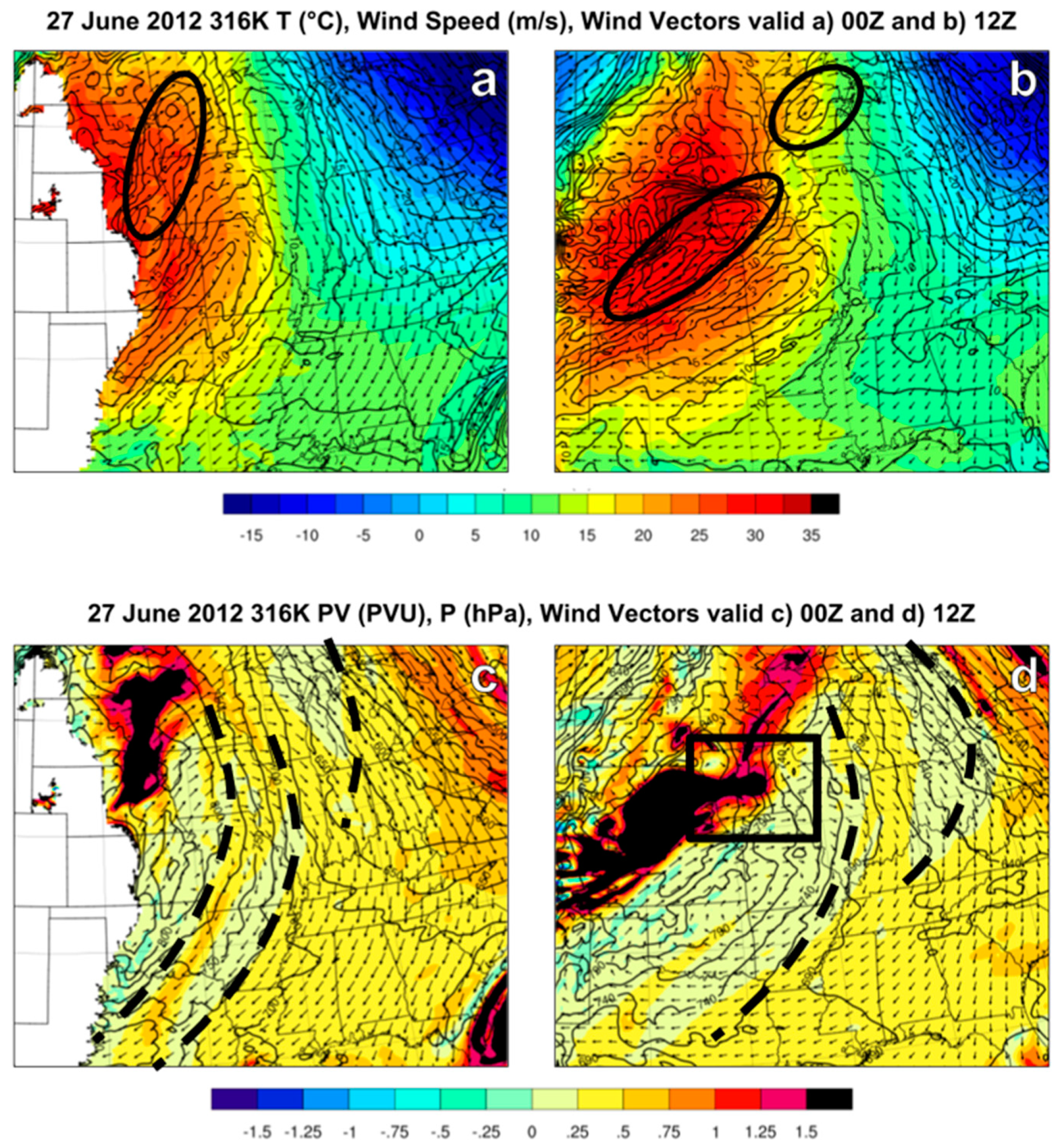
As the hot, dry air and anomalously large mass perturbation advected eastward, along-stream thermally indirect accelerations in the mid-levels of the atmosphere developed in response to the along-stream pressure perturbations established by this warm layer. The along-stream accelerations and overall mass imbalance within the EML on 27 and 28 June eventually resulted in a sustained, ageostrophic mid-level jetlet [48] as depicted in Figure 16, which continued to reinforce and maintain a coherent EMLF in a highly nonlinear process.
3.2.3. 28. June: Mid-Level Mesoscale Jetlet Generation
Beginning after sunrise on 28 June 2012, convergence along the leading edge of the strengthening EMLF over the northern Great Plains became organized and continued to further reinforce the existing, anomalously strong mass perturbation and jetlet. The mid-level jetlet (MLJ) is only somewhat visible on the observed 500 hPa upper air analysis (not shown) due to the coarse-scale of radiosonde observations in space and time. The MLJ is also dwarfed to some extent by the polar jet on the 18 km simulated 500 hPa analyses (not shown). The simulated 316 K isentropic fields in Figure 17 show the MLJ more clearly than the 500 hPa isobaric fields because the jetlet developed in response to the baroclinic-induced mass perturbation along the EMLF, and the EML, in this case, is present mostly between the theta layers of 310 K and 320 K (~333 θe) where the slope of isentropes is concentrated. The 500 hPa layer only cuts through the 316 K layer in limited locations.
The MLJ developed between ~1200 UTC and 1800 UTC with thickness rises along the EMLF which were continuously reinforced by differential vertical motions. As the jetlet propagated eastward around the poleward edge of the ridge, numerous convective events were triggered with the accompanying WAA, surface convergence, and instability coupled with the mutually reinforcing (i.e., moist diabatic heating strengthening the along-stream potential temperature gradients) MLJ and EMLF as they moved downstream.
3.2.4. 28. June: Pre-Derecho Bow Echo(es)
Two smaller bow echoes developed later in the evening on 28 June into early 29 June 2012. The 6 km simulation did generate a persistent, small bowing segment (not shown) earlier on 29 June than was observed (~0000 UTC simulated versus 0400 UTC observed). The 18 km and 6 km simulations capture the environment well, revealing the suspected features that only showed up as weak signals on observational charts. A more detailed analysis of these model results is presented in previous work by the authors [23], but overall, the juxtaposition of the upper-level and mid-level jet streaks and the low-level leading edge of the EMLF is remarkably similar to the larger scale derecho setup that occurred on 29 June, albeit much more limited in spatial extent and intensity.
3.2.5. 29–30 June: The “Super” Derecho
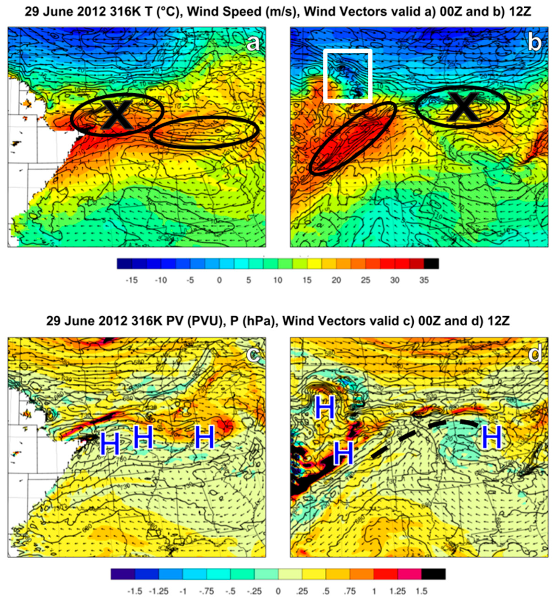
As depicted in Figure 18, an MLJ coupled with the EMLF and associated corridor of high potential static instability (and low inertial stability) moved into the affected region between 0000 UTC and 1200 UTC 29 June 2012. Phasing between the entrance region of the thermally indirect mid-level jetlet and an upper-level divergent polar jet streak right entrance region resulted in sufficient enough lift to initiate deep convection. The EMLF acted as a zone of focused convergence between the poleward polar jet and equatorward mesohigh, creating a well-defined zone of instability for the derecho to travel along.
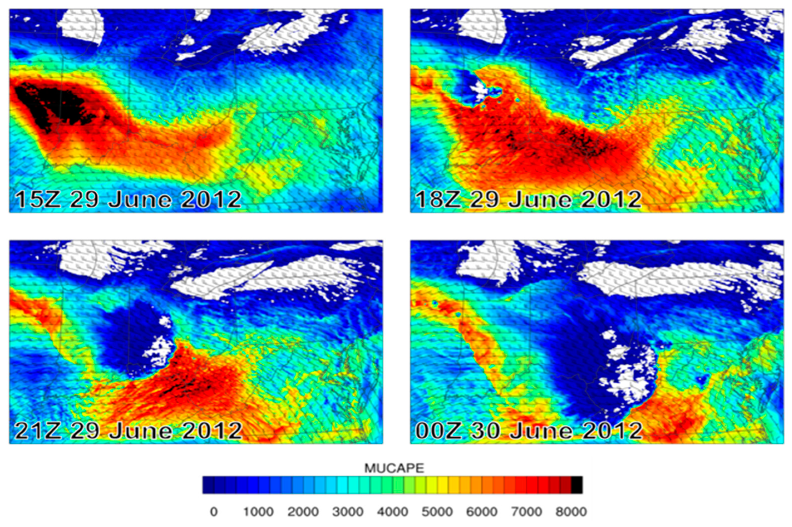
Initial convection with the 29 June 2012 derecho was triggered much earlier in the simulation than in the observations. However, just as in the observed event, once the simulated convection reached the EMLF and associated corridor of high inertial and (potential) static instability (Figure 19), additional convection became explosive (refer back to Figure 11). Once convection was triggered and entered the mesoscale corridor of unique instability, convection worked to reinforce the initial convectively induced cold pool as it continued to propagate downstream while triggering recurrent convection through enhanced surface convergence as the upstream pressure and moist downdrafts accelerated low-level winds.
4. Discussion
While the large-scale (synoptic) setup for derecho-producing events is generally well understood, the issue remains of predicting both if/when a progressive derecho may develop and for how long and far downstream it will propagate. Though an ingredients-based analysis of the synoptic environment on 27–29 June indicated very similar environments and the potential for derechos, the analysis of the meso-β/ɣ simulations presented herein revealed some key mesoscale features involved on 29 June which differentiate the environments on these days. Unfortunately, these features are not consistently captured well with current operational models or observational data.
Over the two weeks of analyses, a unique downscale sequence of dynamics played out leading up to the historic 29 June 2012 event. The origins of the anomalously strong mixed layer which formed over the southwestern U.S. and Mexican Plateau can be traced back at least two weeks to the RWB event on 15–16 June. A record-breaking heatwave began 23 June across the central and western U.S. and lasted well into July 2012. The heat and unusually deep and extensive mixed layer remained in place over the western half of the U.S. until a second RWB event occurred on 26 June. The 26 June RWB triggered the movement of the unusually deep (400+ hPa) mixed layer downstream as the right entrance region of the polar jet streak and mesoscale mass adjustments at the EMLF around the ridge’s periphery worked to separate, deform, and propagate the EML eastward towards the Midwest and Mid-Atlantic by 29 June. In response, on 28 June, there was a final surge of hot Pacific air and diabatic heating over the northern Great Plains which generated a significant mass perturbation that resulted in downstream, along-stream, mid-level accelerations.
The MLJ maintained its structure due to continuous strengthening of the EMLF via both differential moist convective and surface sensible heating. Movement of the EMLF over relatively cooler and more moist air across the Midwest and Mid-Atlantic states created an environment of extreme potential static instability coupled with lowered inertial stability due to the highly anticyclonic nature of the EMLF geometry. As initial convection arrived at the corridor of extreme instability extending nearly 700 miles from Indiana to the Delmarva Peninsula, storms rapidly became north-south oriented and grew upscale into a significant bowing MCS. The 29 June 2012 super derecho continued to propagate and expand upscale along the EMLF interface with the corridor of maximum instability until exiting the continental U.S., where this ideal derecho-producing environment dissipated.
The strength of the EMLF was of particular importance for the 29 June 2012 derecho for numerous reasons, primarily the juxtaposition of high CAPE values with strong DCAPE values for the maintenance of the derecho and associated cold pool downstream and generation of imbalances and subsequent along-stream mid-tropospheric wind maxima. The relative intensities of these features should be of particular interest for the future of derecho forecasting.
The 2 km WRF results presented here indicate that the mesoscale convective triggering processes key in initiating these events happen in the range of 10–15 km. This is because the 4 km NAM (North American Mesoscale Forecast System) did not successfully simulate the derecho, but the operational 3 km HRRR (High-Resolution Weather Research and Forecasting (WRF)-Rapid Refresh) and 2 km WRF-ARW (Advanced Research WRF core) presented in this manuscript quite accurately simulated the derecho, which is consistent with a 5-delta wave mode [49]. These results reinforce the need for higher resolution operational convective allowing models.
Additionally, the use of isentropic analyses along with the more traditional isobaric analyses proved very useful in diagnosing the differences in the environment across the affected region between 27–29 June, which may be useful in the forecasting of future derecho events. The authors of this paper are in the process of conducting high-resolution modeling and analysis of additional derecho events to further investigate the findings presented herein.
Author Contributions
Conceptualization, M.L.K. and K.N.S.; methodology, M.L.K. and K.N.S.; software, K.N.S.; validation, M.L.K. and K.N.S.; formal analysis, M.L.K. and K.N.S.; investigation, K.N.S.; resources, M.L.K.; data curation, K.N.S.; writing—original draft preparation, K.N.S.; writing—review and editing, M.L.K.; visualization, K.N.S.; supervision, M.L.K.; project administration, M.L.K. All authors have read and agreed to the published version of the manuscript.
Funding
This research received no external funding.
Conflicts of Interest
The authors declare no conflict of interest.
References
- SPC Filtered Storm Reports for 06/29/2012. SPC Severe Weather Event Review for Friday 29 June 2012. Available online: www.spc.noaa.gov/exper/archive/event.php?date=20120629 (accessed on 21 August 2021).
- NOAA. The Historic Derecho of 29 June 2012; Service Assessment, U.S. Department of Commerce, NOAA National Weather Service: Silver Spring, MD, USA, 2013; p. 61. [Google Scholar]
- Bentley, E.S.; Jeff, L. An Examination of the Mesoscale Environment and Evolution of the Northern Indiana/Northwest Ohio Derecho of 29 June 2012. Electron. J. Sev. Storms Meteorol. (EJSSM) 2016, 11, 1–25. [Google Scholar]
- Storm Prediction Center Mesoscale Discussion 1304. Available online: https://www.spc.noaa.gov/products/md/2012/md1304.html (accessed on 30 May 2021).
- Johns, R.H.; Hirt, W.D. Derechos: Widespread Convectively Induced Windstorms. Weather Forecast. 1987, 2, 32–49. [Google Scholar] [CrossRef]
- Corfidi1, S.F.; Coniglio, M.C.; Cohen, A.E.; Mead, C.M. A Proposed Revision to the Definition of “Derecho”. Bull. Am. Meteorol. Soc. 2016, 97, 935–949. [Google Scholar] [CrossRef]
- Coniglio, M.C.; Stensrud, D.J.; Richman, M.B. An Observational Study of Derecho-Producing Convective Systems. Weather Forecast. 2004, 19, 320–337. [Google Scholar] [CrossRef]
- Guastini, C.T.; Bosart, L.F. Analysis of a Progressive Derecho Climatology and Associated Formation Environments. Mon. Weather Rev. 2016, 144, 1363–1382. [Google Scholar] [CrossRef]
- Bentley, M.L.; Thomas, L.M. A Climatology of Derecho-Producing Mesoscale Convective Systems in the Central and Eastern United States, 1986–1995. Part I: Temporal and Spatial Distribution. Bull. Am. Meteorol. Soc. 1998, 79, 2527–2540. [Google Scholar] [CrossRef] [Green Version]
- Coniglio, M.C.; Stensrud, D.J. Interpreting the Climatology of Derechos. Weather Forecast. 2004, 19, 595–605. [Google Scholar] [CrossRef] [Green Version]
- Bentley, M.L.; Thomas, L.M.; Stephen, F.B. A synoptic climatology of derecho producing mesoscale convective systems in the north-central plains. Int. J. Climatol. A J. R. Meteorol. Soc. 2000, 20, 1329–1349. [Google Scholar] [CrossRef]
- Johns, R.H. Meteorological Conditions Associated with Bow Echo Development in Convective Storms. Weather Forecast. 1993, 8, 294–299. [Google Scholar] [CrossRef] [Green Version]
- Law, K. A Case Study of Atmospheric Dynamics and Thermodynamics in Derechos and the Societal Impacts. In Atmospheric Hazards—Case Studies in Modeling, Communication, and Societal Impacts; InTech: London, UK, 2016. [Google Scholar]
- Fierro, A.; Gao, J.; Ziegler, C.L.; Mansell, E.R.; MacGorman, D.; Dembek, S.R. Evaluation of a Cloud-Scale Lightning Data Assimilation Technique and a 3DVAR Method for the Analysis and Short-Term Forecast of the 29 June 2012 Derecho Event. Mon. Weather Rev. 2014, 142, 183–202. [Google Scholar] [CrossRef] [Green Version]
- Evans, C.; Weisman, M.L.; Bosart, L.F. Development of an Intense, Warm-Core Mesoscale Vortex Associated with the 8 May 2009 “Super Derecho” Convective Event. J. Atmos. Sci. 2014, 71, 1218–1240. [Google Scholar] [CrossRef]
- Weisman, M.L.; Clark, E.; Lance, B. The 8 May 2009 super derecho: Analysis of a real-time explicit convective forecast. Weather Forecast. 2013, 28, 863–892. [Google Scholar] [CrossRef] [Green Version]
- Dunn, J.L.; Ted, B. Bow echo and mesovortex evolution during the 2 May 2007 North Texas derecho. E-J. Sev. Storms Meteorol. 2011, 6, 1–25. [Google Scholar]
- Metz, N.D.; Bosart, L.F. Derecho and MCS Development, Evolution, and Multiscale Interactions during 3–5 July 2003. Mon. Weather Rev. 2010, 138, 3048–3070. [Google Scholar] [CrossRef]
- Coniglio, M.C.; Corfidi, S.F.; Kain, J.S. Environment and Early Evolution of the 8 May 2009 Derecho-Producing Convective System. Mon. Weather Rev. 2011, 139, 1083–1102. [Google Scholar] [CrossRef] [Green Version]
- Ashley, W.S.; Mote, T.L.; Bentley, M.L. The extensive episode of derecho-producing convective systems in the United States during May and June 1998: A multi-scale analysis and review. Meteorol. Appl. 2007, 14, 227–244. [Google Scholar] [CrossRef]
- Duke, J.W.; Rogash, J.A. Multiscale Review of the Development and Early Evolution of the 9 April 1991 Derecho. Weather Forecast. 1992, 7, 623–635. [Google Scholar] [CrossRef] [Green Version]
- Hinrichs, G.D. Tornadoes and Derechos; Register Publishing Company: Ann Arbor, MI, USA, 1888. [Google Scholar]
- Shourd, K.N. The Multi-Scale Dynamics of the 29–30 June 2012 “Super Derecho”. Master’s Thesis, University of Nevada, Reno, NV, USA, 2017. [Google Scholar]
- Corfidi, S.F.; Evans, J.S.; Johns, R.H.; About Derechos. Facts about Derechos—Very Damaging Windstorms, NOAA NWS Storm Prediction Center. 15 May 2018. Available online: www.spc.noaa.gov/misc/AbtDerechos/derechofacts.htm (accessed on 20 October 2021).
- SPC Severe Weather Events Archive. Available online: https://www.spc.noaa.gov/exper/archive/events/ (accessed on 20 June 2021).
- Atmospheric Soundings. Available online: http://weather.uwyo.edu/upperair/sounding.html (accessed on 20 June 2021).
- Imagery & Data. NOAA National Environmental Satellite, Data, and Information Service (NESDIS), Department of Commerce. Available online: www.nesdis.noaa.gov/content/imagery-data-0 (accessed on 20 June 2021).
- Image Archive: Meteorological Case Study Selection Kit. Available online: https://www2.mmm.ucar.edu/imagearchive/ (accessed on 20 June 2021).
- 29 June 2012 Derecho: The Ohio Valley/Mid-Atlantic Derecho of June 2012. Available online: https://www.spc.noaa.gov/misc/AbtDerechos/casepages/jun292012page.htm (accessed on 20 June 2021).
- Data Tools: Daily Weather Records. Available online: https://www.ncdc.noaa.gov/cdo-web/datatools/records (accessed on 20 June 2021).
- Skamarock, W.C.; Klemp, J.B.; Dudhia, J.; Gill, D.O.; Barker, D.M.; Wang, W.; Powers, J.G.; A Description of the Advanced Research WRF Version 3. NCAR Technical Note-475+ STR. 2008. Available online: https://opensky.ucar.edu/islandora/object/technotes%3A500/datastream/PDF/view (accessed on 9 October 2021).
- NCEP FNL Operational Model Global Tropospheric Analyses, Continuing from July 1999. Available online: https://rda.ucar.edu/datasets/ds083.2/ (accessed on 20 June 2021).
- Thompson, G.; Field, P.R.; Rasmussen, R.M.; Hall, W.D. Explicit Forecasts of Winter Precipitation Using an Improved Bulk Microphysics Scheme. Part II: Implementation of a New Snow Parameterization. Mon. Weather Rev. 2008, 136, 5095–5115. [Google Scholar] [CrossRef]
- Janjic, Z.I. The step-mountain Eta coordinate model: Further developments of the convection, viscous sublayer and turbulence closure schemes. Mon. Wea. Rev. 1994, 122, 927–945. [Google Scholar] [CrossRef] [Green Version]
- Mesinger, F. Forecasting upper tropospheric turbulence within the framework of the Mellor-Yamada 2.5 closure. Res. Activ. Atmos. Ocean. Mod. 1993, 4, 28–29. [Google Scholar]
- Grell, G.A.; Freitas, S.R. A scale and aerosol aware stochastic convective parameterization for weather and air quality modeling. Atmos. Chem. Phys. 2014, 14, 5233–5250. [Google Scholar] [CrossRef] [Green Version]
- Janjic, Z.I. The Surface layer in the NCEP Eta Model. In Proceedings of the Eleventh Conference on Numerical Weather Prediction, Norfolk, VA, USA, 19–23 August 1996; pp. 354–355. [Google Scholar]
- Monin, A.S.; Obukhov, A.M. Basic laws of turbulent mixing in the surface layer of the atmosphere. Contrib. Geophys. Inst. Acad. Sci. USSR 1954, 151, 163–187. (in Russian). [Google Scholar]
- Janjic, Z.I. Nonsingular Implementation of the Mellor-Yamada Level 2.5 Scheme in the NCEP Meso Model; Office Note #437; National Centers for Environmental Prediction: Camp Springs, MD, USA, 2001. [Google Scholar]
- Dudhia, J. Numerical study of convection observed during the Winter Monsoon Experiment using a mesoscale two–dimensional model. J. Atmos. Sci. 1989, 46, 3077–3107. [Google Scholar] [CrossRef]
- Mlawer, E.J.; Taubman, S.J.; Brown, P.D.; Iacono, M.J.; Clough, S.A. Radiative transfer for inhomogeneous atmospheres: RRTM, a validated correlated-k model for the longwave. J. Geophys. Res. Space Phys. 1997, 102, 16663–16682. [Google Scholar] [CrossRef] [Green Version]
- Tewari, M.; Chen, F.; Wang, W.; Dudhia, J.; LeMone, M.A.; Mitchell, K.; Ek, M.; Gayno, G.; Wegiel, J.; Cuenca, R.H. Implementation and verification of the unified NOAH land surface model in the WRF model. In Proceedings of the 20th Conference on Weather Analysis and Forecasting/16th Conference on Numerical Weather Prediction, Seattle, WA, USA, 12 January 2004; pp. 11–15. [Google Scholar]
- Cordeira, J.M.; Metz, N.D.; Howarth, M.E.; Galarneau, T. Multiscale Upstream and In Situ Precursors to the Elevated Mixed Layer and High-Impact Weather over the Midwest United States. Weather Forecast. 2017, 32, 905–923. [Google Scholar] [CrossRef] [Green Version]
- SPC Filtered Storm Reports for 06/28/2012. SPC Severe Weather Event Review for Friday 28 June 2012. Available online: www.spc.noaa.gov/exper/archive/event.php?date=20120628 (accessed on 21 August 2021).
- COD NEXLAB: Satellite and Radar. COD, College of DuPage Meteorology Department. Available online: Weather.cod.edu/satrad/ (accessed on 10 August 2021).
- Maddox, R.A.; Mccollum, D.M.; Howard, K.W. Large-Scale Patterns Associated with Severe Summertime Thunderstorms over Central Arizona. Weather Forecast. 1995, 10, 763–778. [Google Scholar] [CrossRef] [Green Version]
- Orlanski, I. A rational subdivision of scale for atmospheric processes. Bull. Amer. Meteor. Soc. 1975, 56, 527–530. [Google Scholar]
- Kaplan, M.L.; Lin, Y.-L.; Hamilton, D.W.; Rozumalski, R.A. The Numerical Simulation of an Unbalanced Jetlet and Its Role in the Palm Sunday 1994 Tornado Outbreak in Alabama and Georgia. Mon. Weather Rev. 1998, 126, 2133–2165. [Google Scholar] [CrossRef]
- Lin, Y.-L. Mesoscale Dynamics; Cambridge University Press: Cambridge, UK, 2007; Volume 630. [Google Scholar]
Figure 1.
SPC Filtered Storm Reports overlayed on a topographic map of the United States with key geographical features mentioned throughout this study annotated.
Figure 1.
SPC Filtered Storm Reports overlayed on a topographic map of the United States with key geographical features mentioned throughout this study annotated.

Figure 2.
Plot showing the WRF-ARW domains for (a) Simulation 1 and (b) Simulation 2. On panel (a), for Simulation 1, the innermost red polygon labeled “d03” identifies the area covered by domain three, the 2 km simulation. The larger white polygon labeled “d02” shows the area covered by domain two, the 6 km simulation, and the largest, outer map represents area covered by domain one, the 18 km simulation.

Figure 3.
SPC experimental RAP 700–500 hPa (mid-level) lapse rate analyses (°C km−1) for (a) 00Z 26 June, (b) 00Z 27 June, (c) 00Z 28 June, and (d) 00Z 29 June 2012.
Figure 3.
SPC experimental RAP 700–500 hPa (mid-level) lapse rate analyses (°C km−1) for (a) 00Z 26 June, (b) 00Z 27 June, (c) 00Z 28 June, and (d) 00Z 29 June 2012.

Figure 4.
850 hPa temperature (°C) and height (m) analyses from Unisys Weather (original source no longer available) for (a) 00Z 26 June, (b) 00Z 27 June, (c) 00Z 28 June, and (d) 00Z 29 June 2012. The thick black line in each panel indicates the “leading edge” of the EML (i.e., the EMLF).
Figure 4.
850 hPa temperature (°C) and height (m) analyses from Unisys Weather (original source no longer available) for (a) 00Z 26 June, (b) 00Z 27 June, (c) 00Z 28 June, and (d) 00Z 29 June 2012. The thick black line in each panel indicates the “leading edge” of the EML (i.e., the EMLF).

Figure 5.
12Z 29 June 2012 SPC experimental RAP 700–500 hPa analyses of (mid-level) lapse rates (°C km−1). Blue polygon indicates EML over Midwest and Mid-Atlantic states and red “X” indicates core of anomalously strong EML.
Figure 5.
12Z 29 June 2012 SPC experimental RAP 700–500 hPa analyses of (mid-level) lapse rates (°C km−1). Blue polygon indicates EML over Midwest and Mid-Atlantic states and red “X” indicates core of anomalously strong EML.

Figure 6.
12Z 29 June 2012 (a) observed Doppler radar and (b) GOES visible satellite imagery. Red dashed lines on each panel indicate leading edge of EML (or EMLF).
Figure 6.
12Z 29 June 2012 (a) observed Doppler radar and (b) GOES visible satellite imagery. Red dashed lines on each panel indicate leading edge of EML (or EMLF).

Figure 7.
SPC experimental RAP analysis of 15Z 29 June 2012 for (a) surface-based CAPE (red isolines in J kg−1) and CIN (blue shading in J kg−1) values and (b) mixed layer (ML) CAPE and CIN values both in J kg−1.
Figure 7.
SPC experimental RAP analysis of 15Z 29 June 2012 for (a) surface-based CAPE (red isolines in J kg−1) and CIN (blue shading in J kg−1) values and (b) mixed layer (ML) CAPE and CIN values both in J kg−1.

Figure 8.
300 hPa SPC experimental RAP analyses of isoheights (black in m), isotachs (blue fill in kts), and divergence (solid cyan in 10−5 s−1) for (a) 13Z 29 June and (b) 14Z 29 June 2012.
Figure 8.
300 hPa SPC experimental RAP analyses of isoheights (black in m), isotachs (blue fill in kts), and divergence (solid cyan in 10−5 s−1) for (a) 13Z 29 June and (b) 14Z 29 June 2012.

Figure 9.
Panel (a) shows 850 hPa SPC experimental RAP analyses of temperature advection (°C/hour, blue and red fill), heights (m, black lines), temperature (°C, red dashed lines), and wind (black barbs) at 1400 UTC 29 June. Panels b, c, and d show surface-based (SB) CAPE (J kg−1, red lines) and CIN (J kg−1, blue fill) at (b) 1400 UTC, (c) 1600 UTC, and (d) 1800 UTC 29 June 2012.

Figure 10.
Four panel NEXRAD Doppler radar imagery (dBz) for (a) 1453 UTC, (b) 1556 UTC, (c) 1755 UTC, and (d) 1855 UTC on 29 June 2012 [45].
Figure 10.
Four panel NEXRAD Doppler radar imagery (dBz) for (a) 1453 UTC, (b) 1556 UTC, (c) 1755 UTC, and (d) 1855 UTC on 29 June 2012 [45].

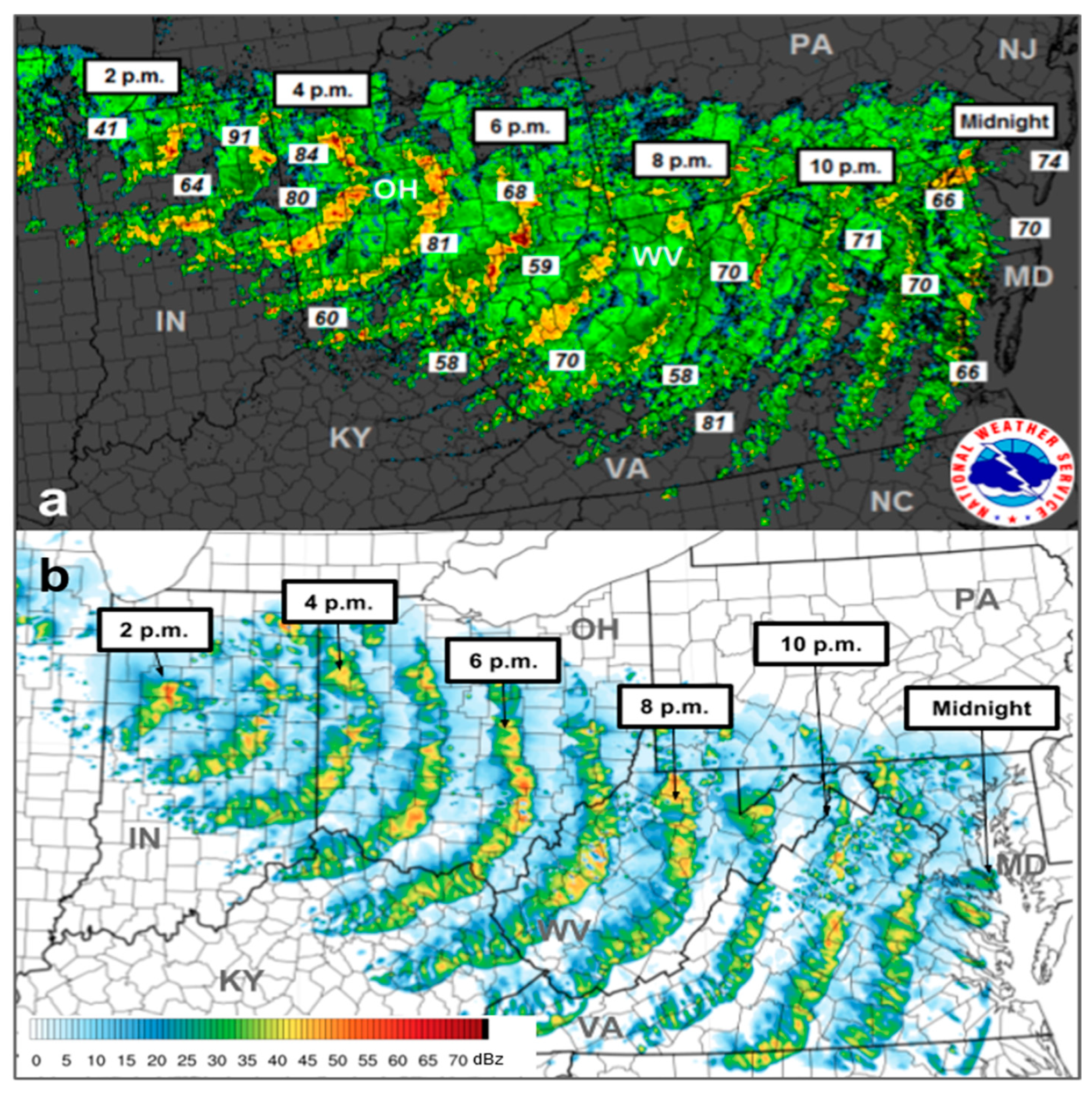
Figure 11.
Comparison of 18Z 29 June through 04Z 30 June 2012 hourly (a) observed composite Doppler radar reflectivity (modified by Greg Carbon [19]) and (b) WRF-ARW 2-km simulated maximum reflectivity (dBz) values.
Figure 11.
Comparison of 18Z 29 June through 04Z 30 June 2012 hourly (a) observed composite Doppler radar reflectivity (modified by Greg Carbon [19]) and (b) WRF-ARW 2-km simulated maximum reflectivity (dBz) values.

Figure 12.
Comparison of the 00Z 25 June 2012 (A) WRF-ARW KDNR 18 km simulated upper air analysis and (B) observed KDNR upper air sounding.
Figure 12.
Comparison of the 00Z 25 June 2012 (A) WRF-ARW KDNR 18 km simulated upper air analysis and (B) observed KDNR upper air sounding.

Figure 13.
Comparison of the 00Z 25 June 2012 (A) WRF-ARW KDDC 18 km simulated upper air analysis and (B) observed KDDC upper air sounding.
Figure 13.
Comparison of the 00Z 25 June 2012 (A) WRF-ARW KDDC 18 km simulated upper air analysis and (B) observed KDDC upper air sounding.

Figure 14.
WRF-ARW 18 km simulated 330 K potential vorticity (fill in PVU (10−6 KhPa−1s−1) and wind barbs (kts) for (a) 12Z 25 June, (b) 00Z 26 June, (c) 12Z 26 June, and (d) 00Z 27 June 2012.
Figure 14.
WRF-ARW 18 km simulated 330 K potential vorticity (fill in PVU (10−6 KhPa−1s−1) and wind barbs (kts) for (a) 12Z 25 June, (b) 00Z 26 June, (c) 12Z 26 June, and (d) 00Z 27 June 2012.

Figure 15.
WRF-ARW 18 km simulated maximum CAPE (MUCAPE, J kg−1) and mean layer wind barbs (kts) (calculated between 0–3000 m AGL) for (a) 00Z 26 June, (b) 00Z 27 June, (c) 00Z 28 June, and (d) 00Z 29 June 2012.
Figure 15.
WRF-ARW 18 km simulated maximum CAPE (MUCAPE, J kg−1) and mean layer wind barbs (kts) (calculated between 0–3000 m AGL) for (a) 00Z 26 June, (b) 00Z 27 June, (c) 00Z 28 June, and (d) 00Z 29 June 2012.

Figure 16.
WRF-ARW 18 km simulated 316 K temperatures (°C, color fill), wind isotachs (black lines in m/s), and wind vectors for (a) 00Z and (b) 12Z 27 June, as well as simulated 316 K potential vorticity (PVU, color fill), pressure (black lines in hPa), and wind vectors valid at (c) 00Z and (d) 12Z 29 June. The white-filled areas in panels (a,c) represent locations where the isentropic surface is interrupted by higher terrain. Black ovals indicate the location(s) of mid-level jetlets (MLJ). The black box shows where along stream perturbations and deformation of the EML are occurring, and black dashed lines indicate surges of the EML eastward out of the main high.

Figure 17.
WRF-ARW 18 km simulated 316 K temperatures (°C, color fill), wind isotachs (black lines in m/s), and wind vectors for (a) 00Z and (b) 12Z 28 June, as well as simulated 316 K potential vorticity (PVU, color fill), pressure (black lines in hPa), and wind vectors valid at (c) 00Z and (d) 12Z 29 June. The white-filled areas in panels (a,c) represent locations where the isentropic surface is interrupted by higher terrain. Black ovals indicate the location(s) of mid-level jetlets (MLJ). Black dashed lines indicate surges of the EML eastwards, and blue “H”s represent meso-highs being ejected from the main EML.

Figure 18.
WRF-ARW 18 km simulated 316 K temperatures (°C, color fill), wind isotachs (black lines in m/s), and wind vectors for (a) 00Z and (b) 12Z 29 June, as well as simulated 316 K potential vorticity (PVU, color fill), pressure (black lines in hPa), and wind vectors valid at (c) 00Z and (d) 12Z 29 June. The white-filled areas in panels (a,c) represent locations where the isentropic surface is interrupted by higher terrain. Black ovals indicate the location(s) of mid-level jetlets (MLJ). Black “X”s indicate the location of the MLJ associated with derecho development. The white box shows the relative location of the cold pool which triggered the derecho. Black dashed lines indicate the EMLF, and blue “H”s represent meso-highs being ejected from the main EML.

Figure 19.
WRF-ARW 2 km simulated maximum CAPE (MUCAPE, fill in J kg−1 between 0–3000 m AGL) and 500 hPa wind barbs (kts) for (top left) 15Z 29 June, (top right) 18Z 29 June, (bottom left) 21Z 29 June, and (bottom right) 00Z 30 June 2012.
Figure 19.
WRF-ARW 2 km simulated maximum CAPE (MUCAPE, fill in J kg−1 between 0–3000 m AGL) and 500 hPa wind barbs (kts) for (top left) 15Z 29 June, (top right) 18Z 29 June, (bottom left) 21Z 29 June, and (bottom right) 00Z 30 June 2012.

Table 2.
Summary of daily and all-time high temperature records from 22 June through 3 July 2012 [30].
Table 2.
Summary of daily and all-time high temperature records from 22 June through 3 July 2012 [30].
| Date | Daily Records | All-Time Records |
|---|---|---|
| 22 June 2012 | 163 | 0 |
| 23 June 2012 | 125 | 2 |
| 24 June 2012 | 196 | 8 |
| 25 June 2012 | 301 | 8 |
| 26 June 2012 | 377 | 14 |
| 27 June 2012 | 337 | 19 |
| 28 June 2012 | 393 | 22 |
| 29 June 2012 | 615 | 55 |
| 30 June 2012 | 655 | 90 |
| 1 July 2012 | 566 | 44 |
| 2 July 2012 | 434 | 20 |
| 3 July 2012 | 304 | 4 |
Publisher’s Note: MDPI stays neutral with regard to jurisdictional claims in published maps and institutional affiliations. |
© 2021 by the authors. Licensee MDPI, Basel, Switzerland. This article is an open access article distributed under the terms and conditions of the Creative Commons Attribution (CC BY) license (https://creativecommons.org/licenses/by/4.0/).
Share and Cite
MDPI and ACS Style
Shourd, K.N.; Kaplan, M.L. The Multiscale Dynamics of the 29 June 2012 Super Derecho. Climate 2021, 9, 155. https://0-doi-org.brum.beds.ac.uk/10.3390/cli9110155
AMA Style
Shourd KN, Kaplan ML. The Multiscale Dynamics of the 29 June 2012 Super Derecho. Climate. 2021; 9(11):155. https://0-doi-org.brum.beds.ac.uk/10.3390/cli9110155
Chicago/Turabian StyleShourd, Kacie Nicole, and Michael L. Kaplan. 2021. "The Multiscale Dynamics of the 29 June 2012 Super Derecho" Climate 9, no. 11: 155. https://0-doi-org.brum.beds.ac.uk/10.3390/cli9110155
Note that from the first issue of 2016, this journal uses article numbers instead of page numbers. See further details here.