
Predicting the Geographic Range of an Invasive Livestock Disease across the Contiguous USA under Current and Future Climate Conditions

 , ,
, ,
Abstract
:1. Introduction
2. Materials and Methods
2.1. VS Occurrence Data
2.2. Approach
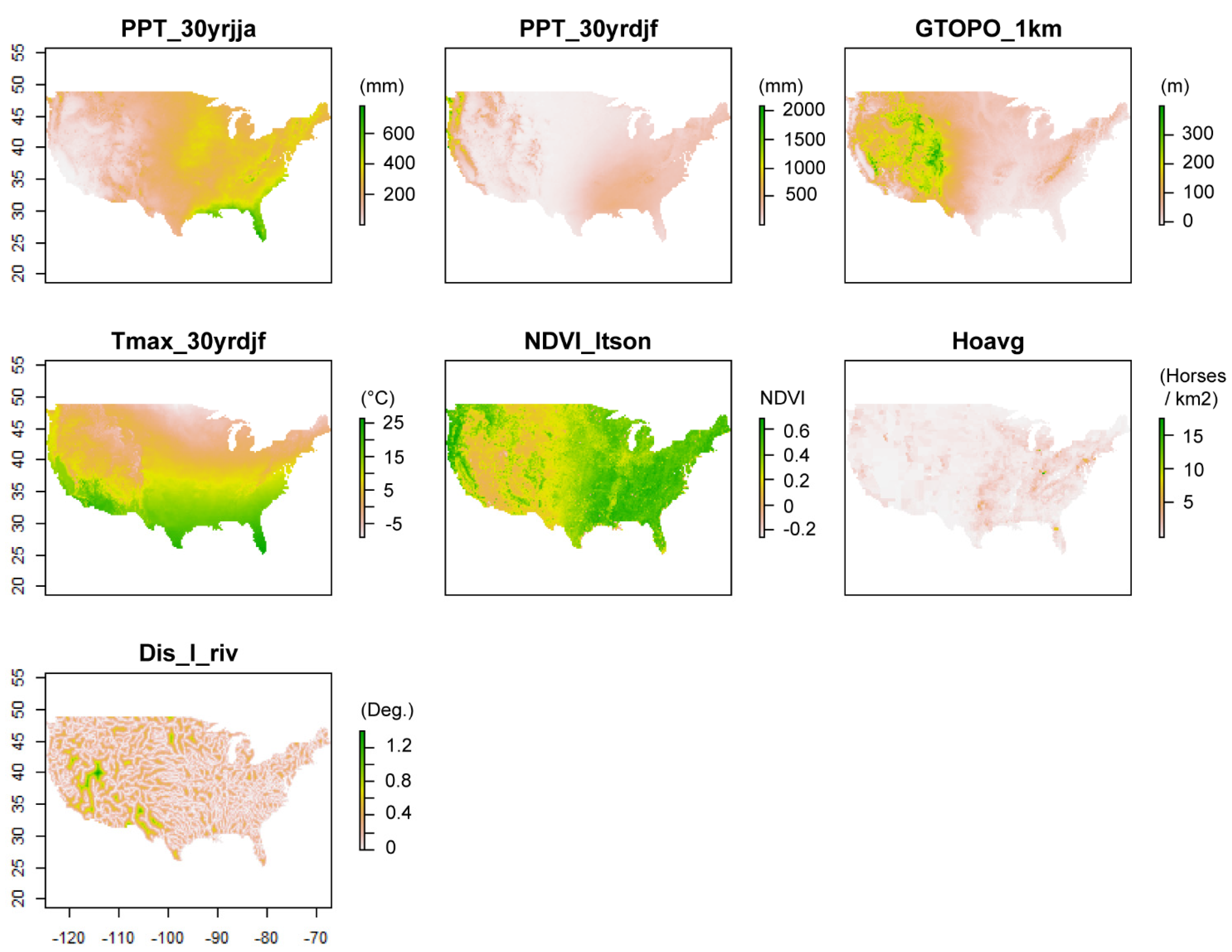
2.3. Data Sources
2.3.1. Current Climate Variables
2.3.2. Hydrology Variables
2.3.3. Land Surface Variables
2.3.4. Biotic Variables
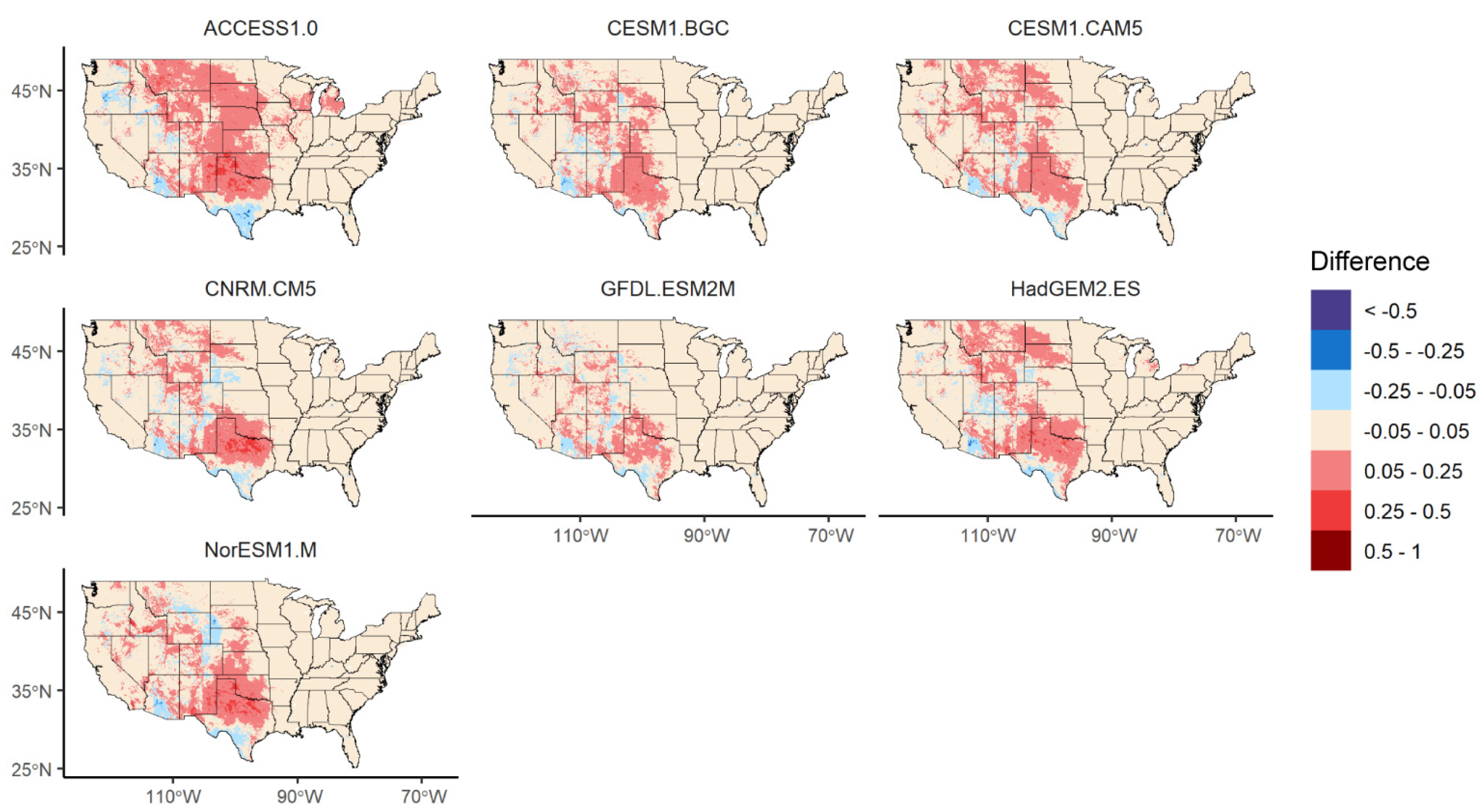
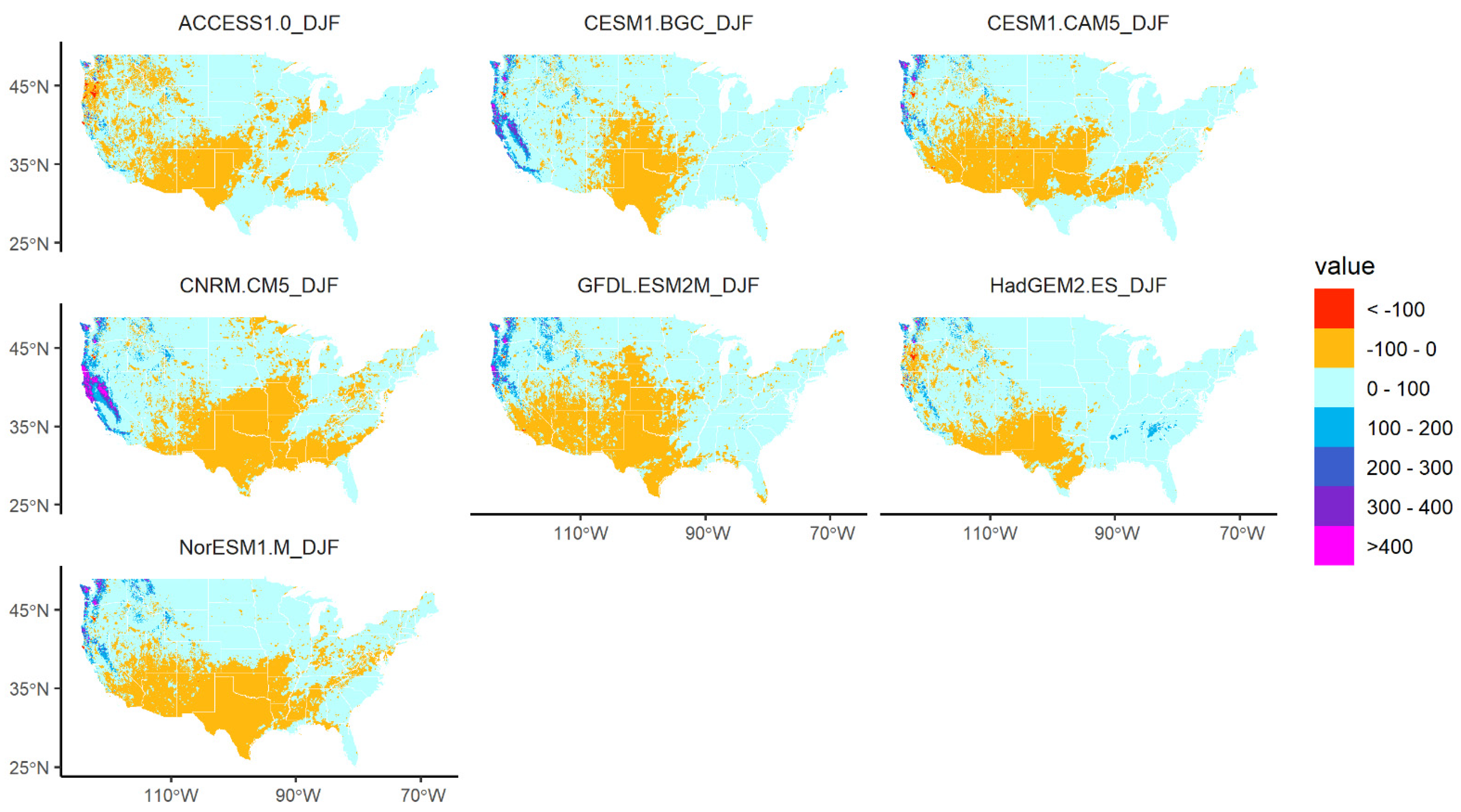
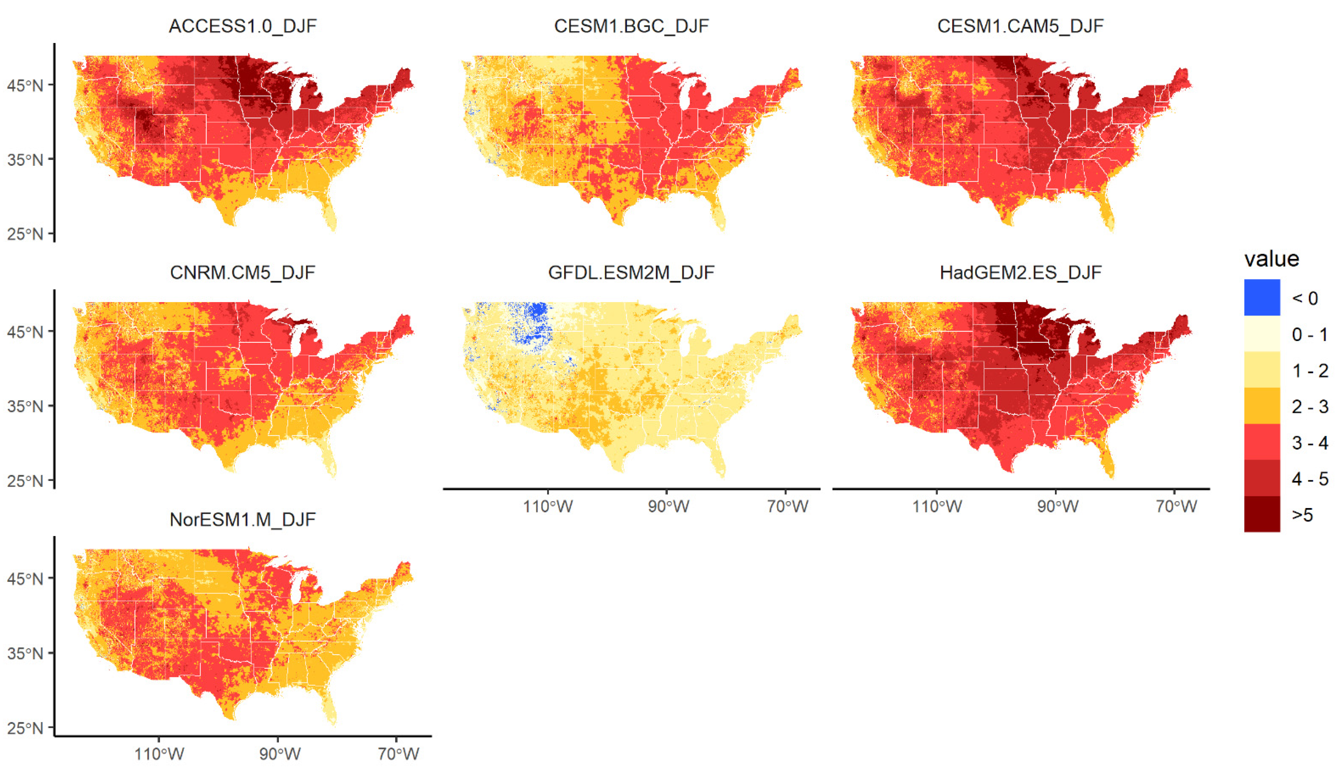
2.4. Future Climate Alternatives
2.5. Analysis
3. Results
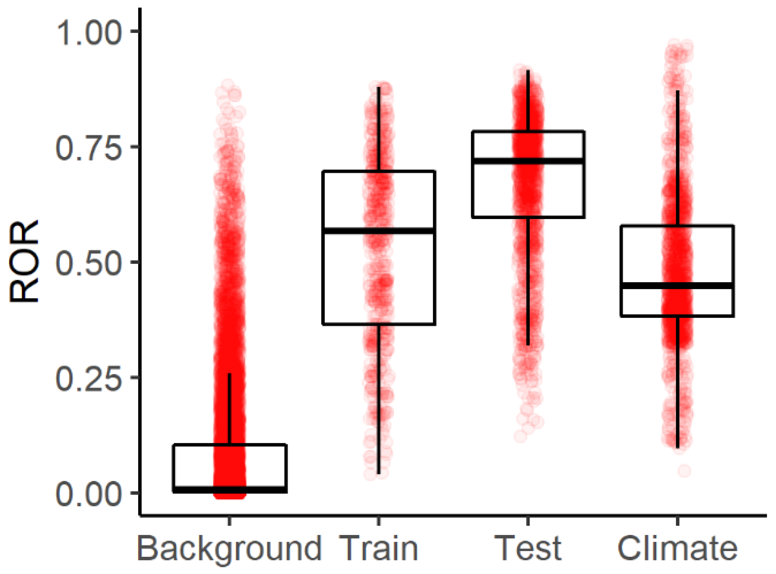
3.1. Model Evaluation
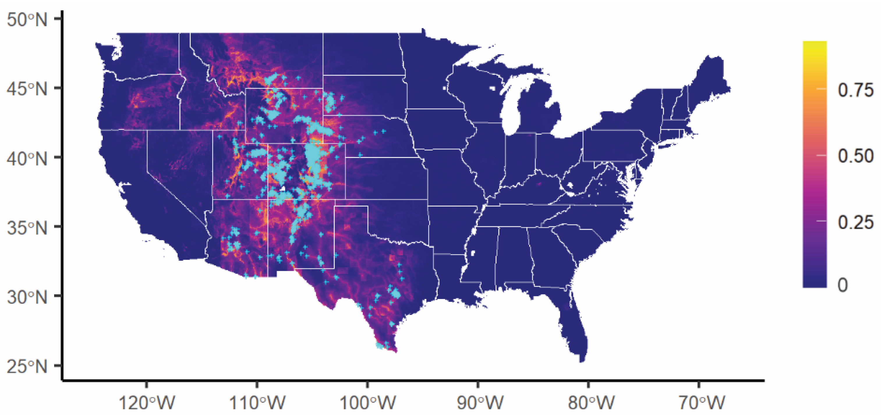
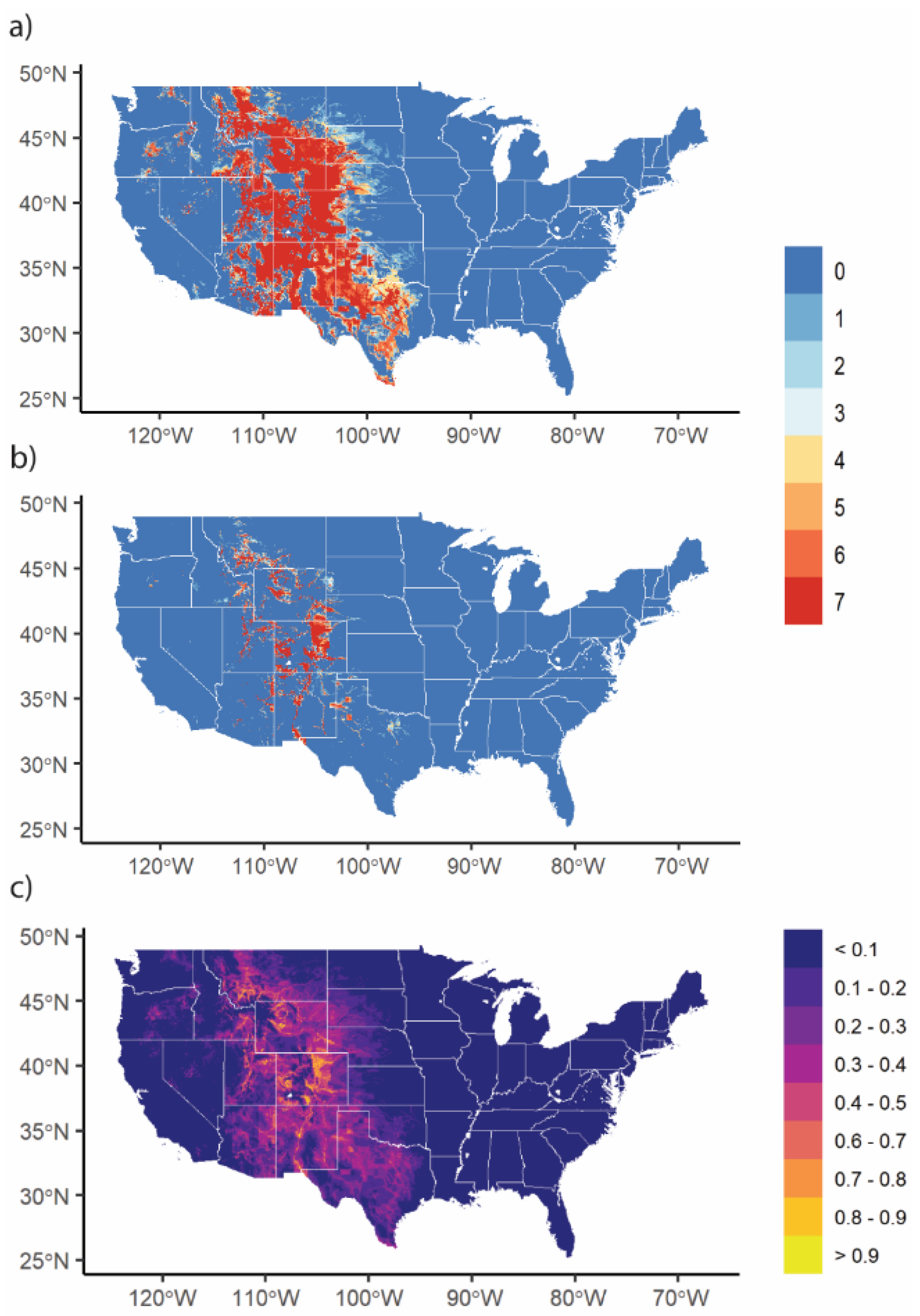
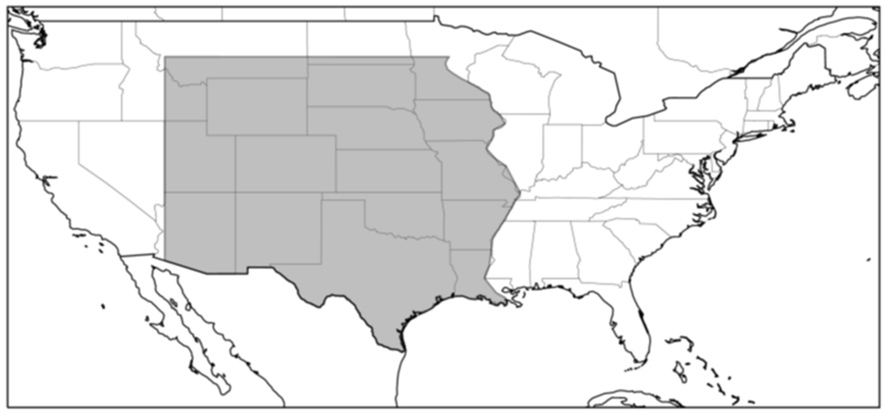
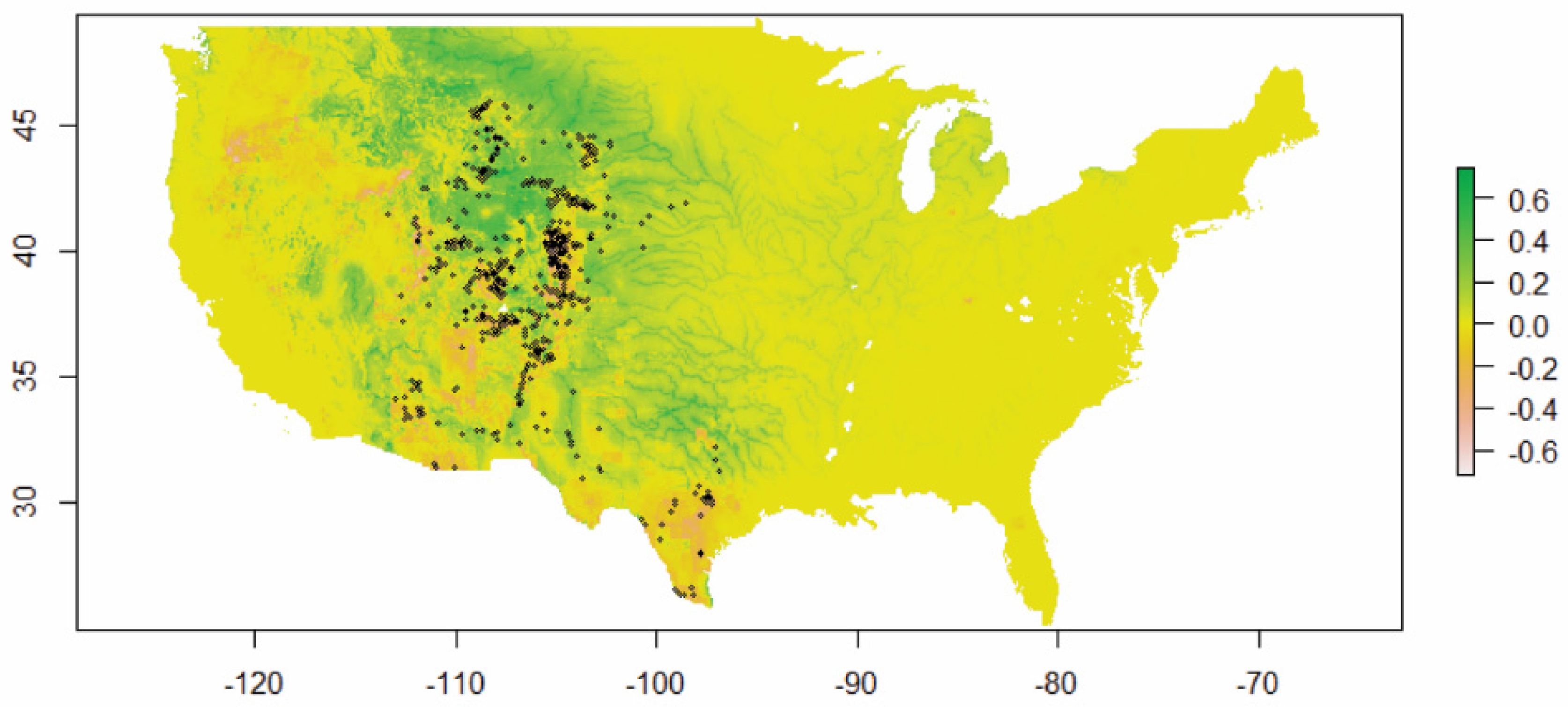
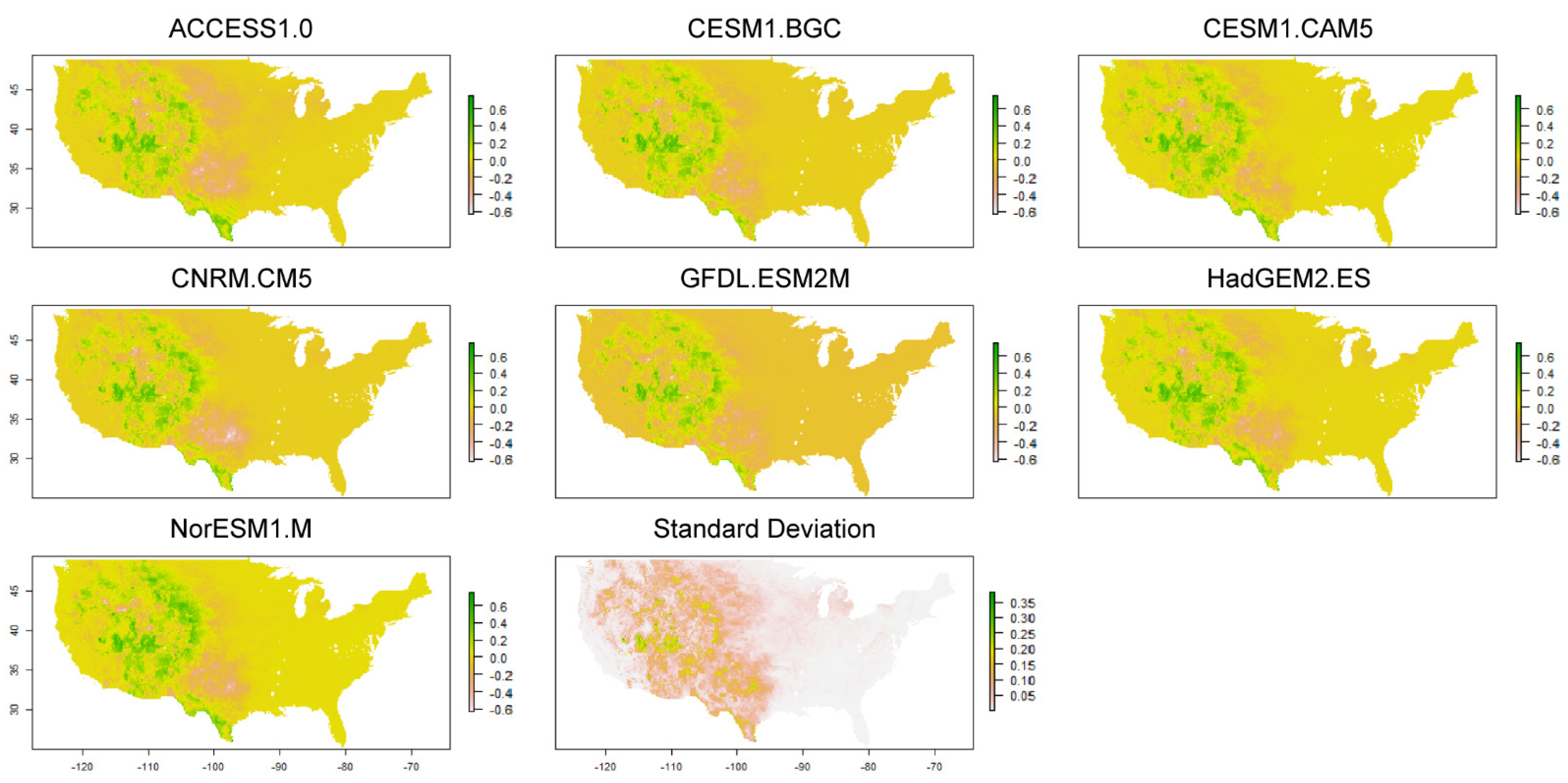
3.2. VS Potential Distribution under Current Climate
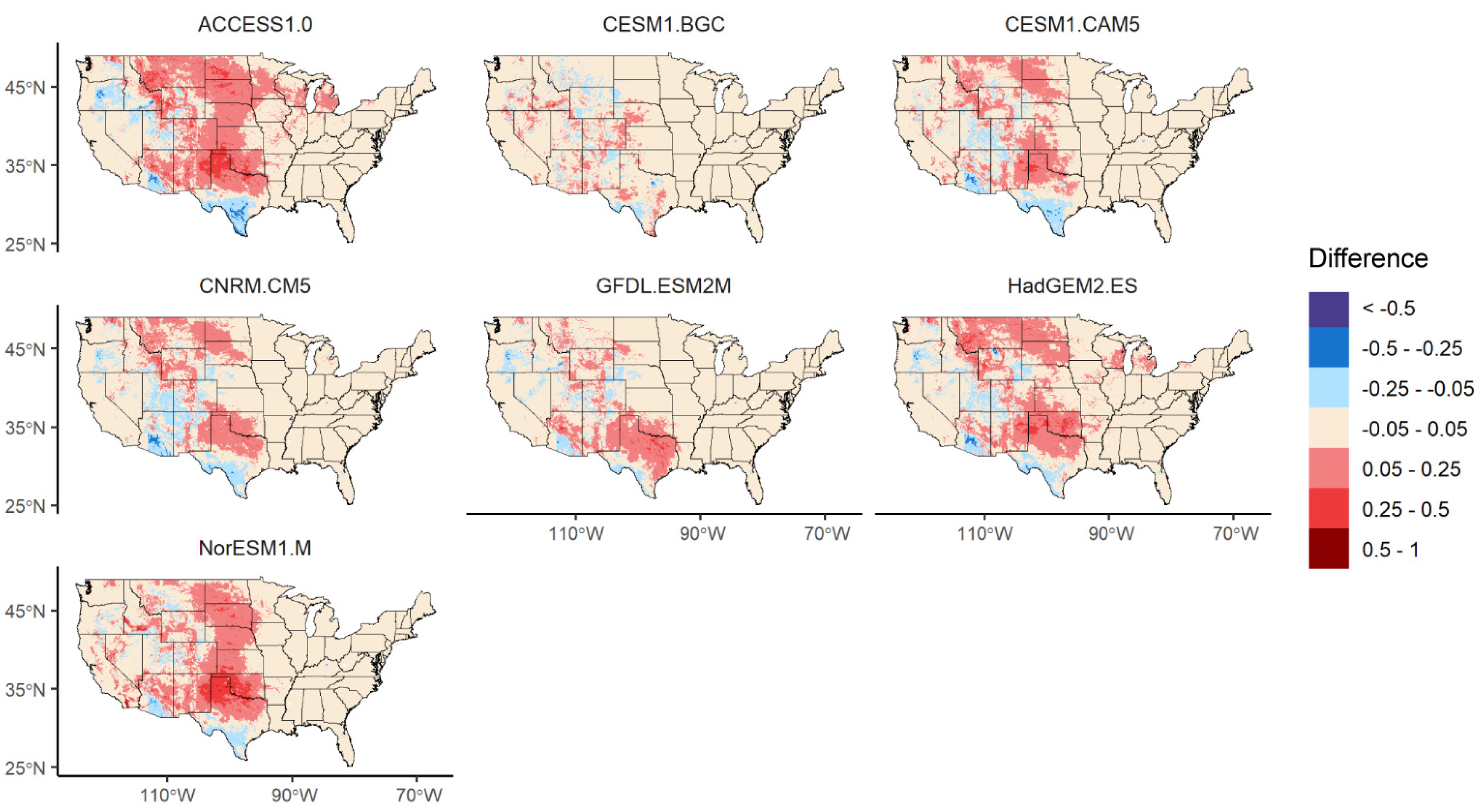
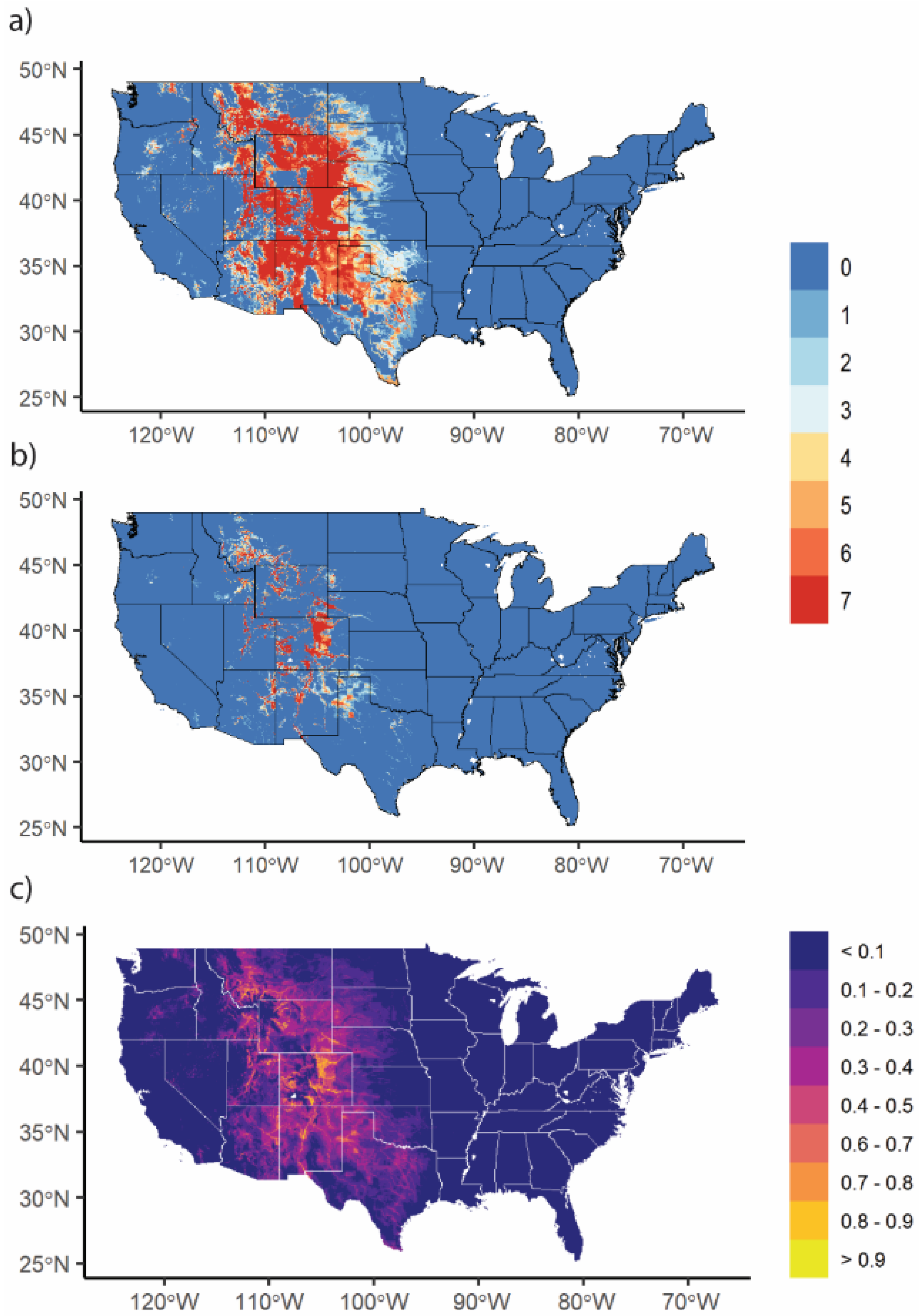
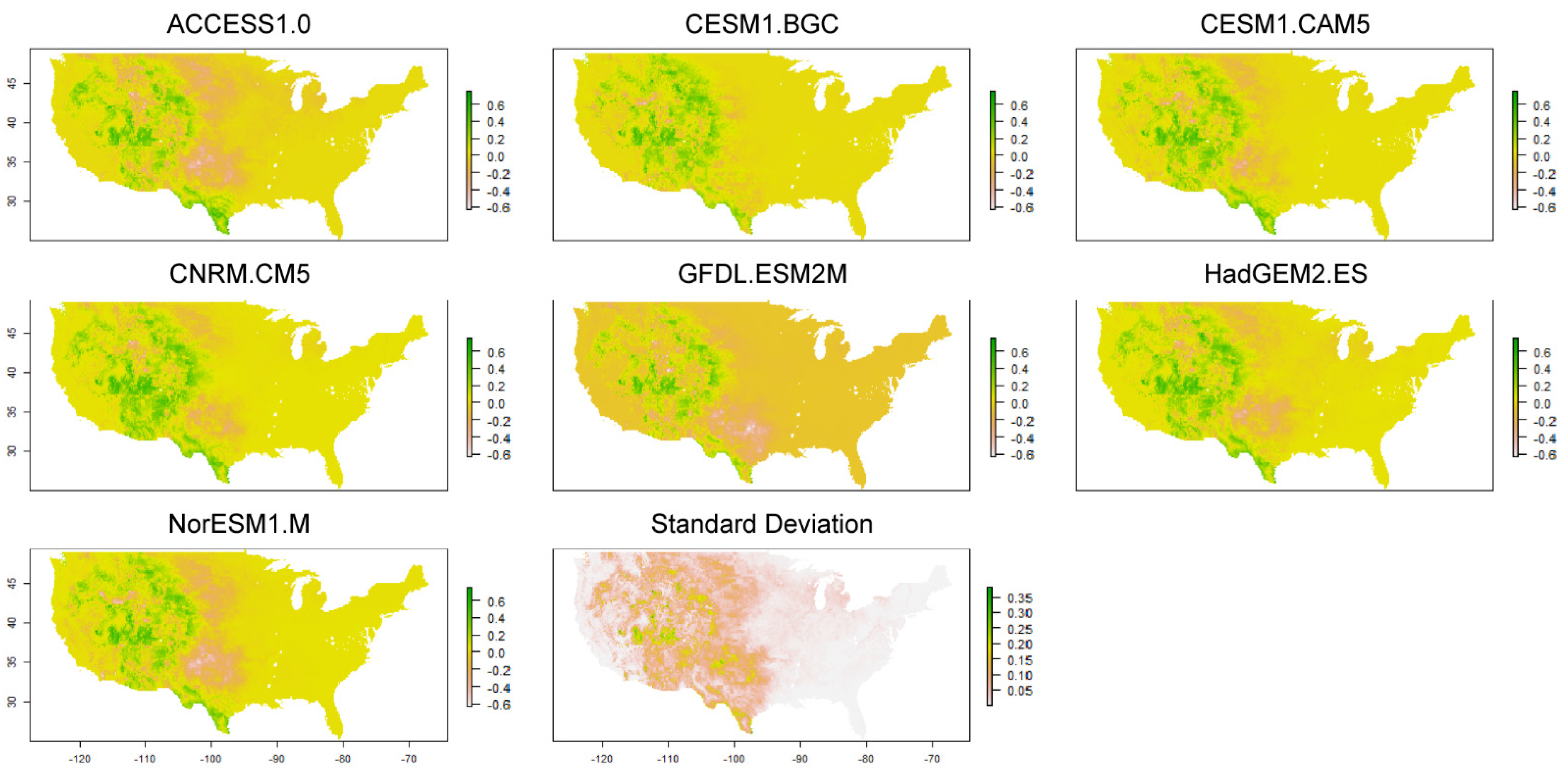
3.3. Changes in Geographic Range under Future Climate Conditions
4. Discussion
5. Conclusions
Author Contributions
Funding
Data Availability Statement
Acknowledgments
Conflicts of Interest
Appendix A


| Metric | Metric Description | Threshold Value of Sufficient Performance |
|---|---|---|
| spatial correlation of climatological pr | A point-by-point Pearson’s r spatial correlation of 100-yr mean pr over the entirety of CONUS. Threshold chosen to eliminate only the worst models. | DJF = 0.6 JJA = 0.6 |
| mean absolute bias in climatological pr | Absolute value of 100-yr mean pr bias, averaged over the evaluation area. Performance thresholds chosen at a break in the bias spread. | DJF = 0.95 mm/day JJA = 1.25 mm/day |
| mean absolute bias in climatological tasmin | Absolute value of 100-yr mean tasmin bias, averaged over the evaluation area. Performance thresholds chosen at a break in the bias spread. | DJF = 4.75 C JJA = 4.0 C |
| mean absolute bias in climatological tasmax | Absolute value of 100-yr mean tasmax bias, averaged over the evaluation area. Performance thresholds chosen at a break in the bias spread. | DJF = 4.25 C JJA = 4.25 C |
| mean absolute bias in pr variability | Absolute value of bias in the standard deviation of detrended anomalies (base period 1906–2005), averaged over the evaluation area. Performance thresholds chosen at a break in the bias spread. | DJF = 0.26 mm/day JJA = 0.35 mm/day |
| mean absolute bias in tasmin variability | Absolute value of bias in the standard deviation of detrended anomalies (base period 1906–2005), averaged over the evaluation area. Performance thresholds chosen at a break in the bias spread. | DJF = 0.7 C JJA = 0.4 C |
| mean absolute bias in tasmax variability | Absolute value of bias in the standard deviation of detrended anomalies (base period 1906-2005), averaged over the evaluation area. Performance thresholds chosen at a break in the bias spread. | DJF = 0.5 C JJA = 0.7 C |
| % of study area with significant bias in 100-yr pr trend | Bias in the 100-yr trend with statistical significance at the 95% significance level computed on the trend of the model minus observations timeseries using a two-tailed students t test. % area computed as number of significant grids divided by total grids in the evaluation area. Performance thesholds chosen to eliminate only the worst performing models. | DJF = 20% of study area JJA = 20% of study area |
| % of study area with significant bias in 100-yr tasmin trend | Bias in the 100-yr trend with statistical significance at the 95% significance level computed on the trend of the model minus observations timeseries using a two-tailed students t test. % area computed as number of significant grids divided by total grids in the evaluation area. Performance thesholds chosen to eliminate only the worst performing models. | DJF = 33.3% of study area JJA = 33.3% of study area |
| % of study area with significant bias in 100-yr tasmax trend | Bias in the 100-yr trend with statistical significance at the 95% significance level computed on the trend of the model minus observations timeseries using a two-tailed students t test. % area computed as number of significant grids divided by total grids in the evaluation area. Performance thesholds chosen to eliminate only the worst performing models. | DJF = 33.3% of study area JJA = 33.3% of study area |
| CMIP5 GCM Name | Modeling Center | Country |
|---|---|---|
| *ACCESS1-0 | Commonwealth Scientific and Industrial Research Organization (CSIRO) and Bureau of Meteorology (BOM), Australia | Australia |
| *ACCESS1-3 | ||
| bcc-csm1-1 | Beijing Climate Center, China Meteorological Administration | China |
| bcc-csm1-1-m | ||
| BNU-ESM | College of Global Change and Earth System Science, Beijing Normal University | China |
| CanESM2 | Canadian Centre for Climate Modelling and Analysis | Canada |
| CCSM4 | National Center for Atmospheric Research | United States |
| *CESM1-BGC | Community Earth System Model Contributors | United States |
| *CESM1-CAM5 | ||
| CMCC-CM | Centro Euro-Mediterraneo per I Cambiamenti Climatici | Italy |
| CMCC-CMS | ||
| *CNRM-CM5 | Centre National de Recherches Météorologiques/Centre Européen de Recherche et Formation Avancée en Calcul Scientifique | France |
| CSIRO-Mk3-6-0 | Commonwealth Scientific and Industrial Research Organization in collaboration with Queensland Climate Change Centre of Excellence | Australia |
| FGOALS-g2 | LASG, Institute of Atmospheric Physics, Chinese Academy of Sciences and CESS, Tsinghua University | China |
| GFDL-CM3 | NOAA Geophysical Fluid Dynamics Laboratory | United States |
| GFDL-ESM2G | ||
| *GFDL-ESM2M | ||
| GISS-E2-H | NASA Goddard Institute for Space Studies | United States |
| GISS-E2-H-CC | ||
| GISS-E2-R | ||
| GISS-E2-R-CC | ||
| HadGEM2-CC | Met Office Hadley Centre (additional HadGEM2-ES realizations contributed by Instituto Nacional de Pesquisas Espaciais) | United Kingdom |
| *HadGEM2-ES | ||
| inmcm4 | Institute for Numerical Mathematics | Russia |
| IPSL-CM5A-LR | Institut Pierre-Simon Laplace | France |
| IPSL-CM5A-MR | ||
| IPSL-CM5B-LR | ||
| MIROC5 | Atmosphere and Ocean Research Institute (The University of Tokyo), National Institute for Environmental Studies, and Japan Agency for Marine-Earth Science and Technology | Japan |
| MIROC-ESM | Japan Agency for Marine-Earth Science and Technology, Atmosphere and Ocean Research Institute (The University of Tokyo), and National Institute for Environmental Studies | Japan |
| MIROC-ESM-CHEM | ||
| MPI-ESM-LR | Max-Planck-Institut für Meteorologie (Max Planck Institute for Meteorology) | Germany |
| MPI-ESM-MR | ||
| MRI-CGCM3 | Meteorological Research Institute | Japan |
| NorESM1-M | Norwegian Climate Centre | Norway |
References
- Woolhouse, M.E.J.; Gowtage-Sequeria, S. Host Range and Emerging and Reemerging Pathogens. Emerg. Infect. Dis. 2005, 11, 1842–1847. [Google Scholar] [CrossRef] [PubMed]
- Ostfeld, R.S. Climate change and the distribution and intensity of infectious diseases. Ecology 2009, 90, 903–905. [Google Scholar] [CrossRef] [Green Version]
- Gage, K.L.; Burkot, T.R.; Eisen, R.J.; Hayes, E.B. Climate and Vectorborne Diseases. Am. J. Prev. Med. 2008, 35, 436–450. [Google Scholar] [CrossRef] [PubMed]
- Caminade, C.; McIntyre, K.M.; Jones, A.E. Impact of recent and future climate change on vector-borne diseases. Ann. N. Y. Acad. Sci. 2019, 1436, 157–173. [Google Scholar] [CrossRef] [Green Version]
- Morand, S.; Lajaunie, C. Outbreaks of Vector-Borne and Zoonotic Diseases Are Associated With Changes in Forest Cover and Oil Palm Expansion at Global Scale. Front. Vet. Sci. 2021, 8, 230. [Google Scholar] [CrossRef]
- Wimberly, M.C.; Davis, J.K.; Evans, M.V.; Hess, A.; Newberry, P.M.; Solano-Asamoah, N.; Murdock, C.C. Land cover affects microclimate and temperature suitability for arbovirus transmission in an urban landscape. PLoS Negl. Trop. Dis. 2020, 14, e0008614. [Google Scholar] [CrossRef]
- Murdock, C.C.; Evans, M.V.; McClanahan, T.D.; Miazgowicz, K.L.; Tesla, B. Fine-scale variation in microclimate across an urban landscape shapes variation in mosquito population dynamics and the potential of Aedes albopictus to transmit arboviral disease. PLoS Negl. Trop. Dis. 2017, 11, e0005640. [Google Scholar] [CrossRef] [PubMed] [Green Version]
- LaDeau, S.L.; Allan, B.F.; Leisnham, P.T.; Levy, M.Z. The ecological foundations of transmission potential and vector-borne disease in urban landscapes. Funct. Ecol. 2015, 29, 889–901. [Google Scholar] [CrossRef] [PubMed] [Green Version]
- Peters, D.P.C.; McVey, D.S.; Elias, E.H.; Pelzel-McCluskey, A.M.; Derner, J.D.; Burruss, N.D.; Schrader, T.S.; Yao, J.; Pauszek, S.J.; Lombard, J.; et al. Big data–model integration and AI for vector-borne disease prediction. Ecosphere 2020, 11. [Google Scholar] [CrossRef]
- Parham, P.E.; Waldock, J.; Christophides, G.K.; Hemming, D.; Agusto, F.; Evans, K.J.; Fefferman, N.; Gaff, H.; Gumel, A.; LaDeau, S.; et al. Climate, environmental and socio-economic change: Weighing up the balance in vector-borne disease transmission. Philos. Trans. R. Soc. B Biol. Sci. 2015, 370, 20130551. [Google Scholar] [CrossRef] [Green Version]
- Racloz, V.; Ramsey, R.; Tong, S.; Hu, W. Surveillance of Dengue Fever Virus: A Review of Epidemiological Models and Early Warning Systems. PLoS Negl. Trop. Dis. 2012, 6, e1648. [Google Scholar] [CrossRef] [Green Version]
- Peters, D.P.C.; Burruss, N.D.; Rodriguez, L.L.; McVey, D.S.; Elias, E.H.; Pelzel-McCluskey, A.M.; Derner, J.D.; Schrader, T.S.; Yao, J.; Pauszek, S.J.; et al. An Integrated View of Complex Landscapes: A Big Data-Model Integration Approach to Transdisciplinary Science. Bioscience 2018, 68, 653–669. [Google Scholar] [CrossRef]
- Altizer, S.; Ostfeld, R.S.; Johnson, P.T.J.; Kutz, S.; Harvell, C.D. Climate Change and Infectious Diseases: From Evidence to a Predictive Framework. Science 2013, 341, 514–519. [Google Scholar] [CrossRef] [Green Version]
- Campbell-Lendrum, D.; Manga, L.; Bagayoko, M.; Sommerfeld, J. Climate change and vector-borne diseases: What are the implications for public health research and policy? Philos. Trans. R. Soc. B Biol. Sci. 2015, 370, 20130552. [Google Scholar] [CrossRef] [Green Version]
- Lafferty, K.D. Calling for an ecological approach to studying climate change and infectious diseases. Ecology 2009, 90, 932–933. [Google Scholar] [CrossRef] [PubMed]
- Greer, A.; Ng, V.; Fisman, D. Climate change and infectious diseases in North America: The road ahead. Cmaj 2008, 178, 715–722. [Google Scholar] [PubMed] [Green Version]
- Epstein, P.R. Climate change and emerging infectious diseases. Microbes Infect. 2001, 3, 747–754. [Google Scholar] [CrossRef]
- Randolph, S.E.; Rogers, D.J. Tick-borne Disease Systems: Mapping Geographic and Phylogenetic Space. Adv. Parasitol. 2006, 62, 263–291. [Google Scholar]
- Han, B.A.; Drake, J.M. Future directions in analytics for infectious disease intelligence. EMBO Rep. 2016, 17, 785–789. [Google Scholar] [CrossRef] [Green Version]
- Stephens, P.R.; Altizer, S.; Smith, K.F.; Alonso Aguirre, A.; Brown, J.H.; Budischak, S.A.; Byers, J.E.; Dallas, T.A.; Jonathan Davies, T.; Drake, J.M.; et al. The macroecology of infectious diseases: A new perspective on global-scale drivers of pathogen distributions and impacts. Ecol. Lett. 2016, 19, 1159–1171. [Google Scholar] [CrossRef] [PubMed] [Green Version]
- de Araújo, C.B.; Marcondes-Machado, L.O.; Costa, G.C. The importance of biotic interactions in species distribution models: A test of the Eltonian noise hypothesis using parrots. J. Biogeogr. 2014, 41, 513–523. [Google Scholar] [CrossRef]
- Berkelman, R.L.; Bryan, R.T.; Osterholm, M.T.; LeDuc, J.W.; Hughes, J.M. Infectious disease surveillance: A crumbling foundation. Science 1994, 264, 368–370. [Google Scholar] [CrossRef] [PubMed] [Green Version]
- Intergovernmental Panel on Climate Change IPCC Special Report: Emissions Scenarios; Cambridge University: Cambridge, UK, 2000.
- Stouffer, R.J.; Weaver, A.J.; Eby, M. A method for obtaining pre-twentieth century initial conditions for use in climate change studies. Clim. Dyn. 2004, 23, 327–339. [Google Scholar] [CrossRef]
- Taylor, K.E.; Stouffer, R.J.; Meehl, G.A. An Overview of CMIP5 and the Experiment Design. Bull. Am. Meteorol. Soc. 2012, 93, 485–498. [Google Scholar] [CrossRef] [Green Version]
- Geil, K.L. Assessing the 20th Century Performance of Global Climate Models and Application to Climate Change Adaptation Planning. Ph.D. Thesis, The University of Arizona, Tucson, AZ, USA, 2017. [Google Scholar]
- Knutti, R. The end of model democracy? Clim. Change 2010, 102, 395–404. [Google Scholar] [CrossRef]
- Barsugli, J.J.; Guentchev, G.; Horton, R.M.; Wood, A.; Mearns, L.O.; Liang, X.-Z.; Winkler, J.A.; Dixon, K.; Hayhoe, K.; Rood, R.B.; et al. The Practitioner’s Dilemma: How to Assess the Credibility of Downscaled Climate Projections. Eos Trans. Am. Geophys. Union 2013, 94, 424–425. [Google Scholar] [CrossRef] [Green Version]
- Knutti, R.; Furrer, R.; Tebaldi, C.; Cermak, J.; Meehl, G.A. Challenges in Combining Projections from Multiple Climate Models. J. Clim. 2010, 23, 2739–2758. [Google Scholar] [CrossRef] [Green Version]
- Nissan, H.; Goddard, L.; de Perez, E.C.; Furlow, J.; Baethgen, W.; Thomson, M.C.; Mason, S.J. On the use and misuse of climate change projections in international development. Wiley Interdiscip. Rev. Clim. Chang. 2019, 10, e579. [Google Scholar] [CrossRef] [Green Version]
- Whetton, P.; Macadam, I.; Bathols, J.; O’Grady, J. Assessment of the use of current climate patterns to evaluate regional enhanced greenhouse response patterns of climate models. Geophys. Res. Lett. 2007, 34, L14701. [Google Scholar] [CrossRef]
- Rodriguez, L.L.; Bunch, T.A.; Fraire, M.; Llewellyn, Z.N. Re-emergence of Vesicular Stomatitis in the Western United States Is Associated with Distinct Viral Genetic Lineages. Virology 2000, 271, 171–181. [Google Scholar] [CrossRef] [Green Version]
- Rodríguez, L.L. Emergence and re-emergence of vesicular stomatitis in the United States. Virus Res. 2002, 85, 211–219. [Google Scholar] [CrossRef]
- Jamal, S.M.; Belsham, G.J. Foot-and-mouth disease: Past, present and future. Vet. Res. 2013, 44, 116. [Google Scholar] [CrossRef] [Green Version]
- McVicar, J.W.; Sutmoller, P.; Ferris, D.H.; Campbell, C.H. Foot-and-mouth disease in white-tailed deer: Clinical signs and transmission in the laboratory. In Proceedings of the Proceedings, Annual Meeting of the United States Animal Health Association, Roanoke, VA, USA, 13–18 October 1974; pp. 169–180. [Google Scholar]
- Ogden, N.H.; St-Onge, L.; Barker, I.K.; Brazeau, S.; Bigras-Poulin, M.; Charron, D.F.; Francis, C.M.; Heagy, A.; Lindsay, R.; Maarouf, A.; et al. Risk maps for range expansion of the Lyme disease vector, Ixodes scapularis, in Canada now and with climate change. Int. J. Health Geogr. 2008, 7, 24. [Google Scholar] [CrossRef] [Green Version]
- Taylor, S.W.; Safanyik, L. Effect of climate change on range expansion by the mountain pine beetle in British Columbia. In Mountain Pine Beetle Symposium: Challenges and Solutions; Canadian Forest Service: Victoria, BC, Canada, 2003. [Google Scholar]
- Anderson, D.R. Model Based Inference in the Life Sciences: A Primer on Evidence; Springer: New York, NY, USA, 2008. [Google Scholar]
- Elias, E.; McVey, D.S.; Peters, D.; Derner, J.D.; Pelzel-McCluskey, A.; Schrader, T.S.; Rodriguez, L. Contributions of Hydrology to Vesicular Stomatitis Virus Emergence in the Western USA. Ecosystems 2019, 22, 416–433. [Google Scholar] [CrossRef]
- La Sorte, F.A.; Jetz, W. Avian distributions under climate change: Towards improved projections. J. Exp. Biol. 2010, 213, 862–869. [Google Scholar] [CrossRef] [PubMed] [Green Version]
- PRISM Climate Group PRISM Climate Data. Available online: http://prism.oregonstate.edu (accessed on 15 November 2018).
- Hertig, E. Distribution of Anopheles vectors and potential malaria transmission stability in Europe and the Mediterranean area under future climate change. Parasit. Vectors 2019, 12, 18. [Google Scholar] [CrossRef] [PubMed] [Green Version]
- Kramer, L.D. Complexity of virus–vector interactions. Curr. Opin. Virol. 2016, 21, 81–86. [Google Scholar] [CrossRef] [Green Version]
- Botto, C.; Escalona, E.; Vivas-Martinez, S.; Behm, V.; Delgado, L.; Coronel, P. Geographical patterns of onchocerciasis in southern Venezuela: Relationships between environment and infection prevalence. Parassitologia 2005, 47, 145–150. [Google Scholar]
- Lambrechts, L.; Paaijmans, K.P.; Fansiri, T.; Carrington, L.B.; Kramer, L.D.; Thomas, M.B.; Scott, T.W. Impact of daily temperature fluctuations on dengue virus transmission by Aedes aegypti. Proc. Natl. Acad. Sci. USA 2011, 108, 7460–7465. [Google Scholar] [CrossRef] [PubMed] [Green Version]
- Davis, C.; Murphy, A.K.; Bambrick, H.; Devine, G.J.; Frentiu, F.D.; Yakob, L.; Huang, X.; Li, Z.; Yang, W.; Williams, G.; et al. A regional suitable conditions index to forecast the impact of climate change on dengue vectorial capacity. Environ. Res. 2021, 195, 110849. [Google Scholar] [CrossRef]
- Baylis, M.; Caminade, C.; Turner, J.; Jones, A.E. The role of climate change in a developing threat: The case of bluetongue in Europe. Rev. Sci. Tech. l’OIE 2017, 36, 467–478. [Google Scholar] [CrossRef] [PubMed] [Green Version]
- Tabachnick, W.J. Challenges in predicting climate and environmental effects on vector-borne disease episystems in a changing world. J. Exp. Biol. 2010, 213, 946–954. [Google Scholar] [CrossRef] [PubMed] [Green Version]
- Gould, E.A.; Higgs, S. Impact of climate change and other factors on emerging arbovirus diseases. Trans. R. Soc. Trop. Med. Hyg. 2009, 103, 109–121. [Google Scholar] [CrossRef] [PubMed] [Green Version]
- Mellor, P.S.; Boorman, J.; Baylis, M. Culicoides Biting Midges: Their Role as Arbovirus Vectors. Annu. Rev. Entomol. 2000, 45, 307–340. [Google Scholar] [CrossRef]
- Erram, D.; Blosser, E.M.; Burkett-Cadena, N. Habitat associations of Culicoides species (Diptera: Ceratopogonidae) abundant on a commercial cervid farm in Florida, USA. Parasit. Vectors 2019, 12, 367. [Google Scholar] [CrossRef] [PubMed] [Green Version]
- Goddard Earth Sciences Data and Information Services Center (GESDISC) GIOVANNI. Available online: https://giovanni.gsfc.nasa.gov/giovanni/#servie=Ou (accessed on 15 November 2018).
- Xia, Y.; Mitchell, K.; Ek, M.; Sheffield, J.; Cosgrove, B.; Wood, E.; Luo, L.; Alonge, C.; Wei, H.; Meng, J.; et al. Continental-scale water and energy flux analysis and validation for the North American Land Data Assimilation System project phase 2 (NLDAS-2): 1. Intercomparison and application of model products. J. Geophys. Res. Atmos. 2012, 117, D3. [Google Scholar] [CrossRef]
- Kettle, D.S. Ceratopogonidae (Biting midges). In Medical and Veterinary Entomology; Croom Helm: Sydney, Australia, 1984; pp. 137–158. [Google Scholar]
- Lillie, T.H.; Marquardt, W.C.; Jones, R.H. The Flight Range of Culicoides Variipennis (Diptera: Ceratopogonidae). Can. Entomol. 1981, 113, 419–426. [Google Scholar] [CrossRef]
- U.S. Geological Survey. North American Rivers and Lakes. Available online: https://www.sciencebase.gov/catalog/item/4fb55df0e4b04cb937751e02 (accessed on 31 May 2018).
- Kaneene, J.B.; Bruning-Fann, C.S.; Granger, L.M.; Miller, R.; Porter-Spalding, B.A. Environmental and farm management factors associated with tuberculosis on cattle farms in northeastern Michigan. J. Am. Vet. Med. Assoc. 2002, 221, 837–842. [Google Scholar] [CrossRef] [Green Version]
- U.S. Geological Survey Gap Analysis Program GAP/LANDFIRE National Terrestrial Ecosystems 2011; U.S. Geological Survey: Boise, ID, USA, 2016.
- Baylis, M.; Rawlings, P. Modelling the distribution and abundance of Culicoides imicola in Morocco and Iberia using climatic data and satellite imagery. In African Horse Sickness; Springer: Vienna, Austria, 1998; pp. 137–153. [Google Scholar]
- Baylis, M.; Meiswinkel, R.; Venter, G.J. A preliminary attempt to use climate data and satellite imagery to model the abundance and distribution of Culicoides imicola (Diptera: Ceratopogonidae) in southern Africa. J. S. Afr. Vet. Assoc. 1999, 70, 80–89. [Google Scholar] [CrossRef] [PubMed] [Green Version]
- Sloyer, K.E.; Burkett-Cadena, N.D.; Yang, A.; Corn, J.L.; Vigil, S.L.; McGregor, B.L.; Wisely, S.M.; Blackburn, J.K. Ecological niche modeling the potential geographic distribution of four Culicoides species of veterinary significance in Florida, USA. PLoS ONE 2019, 14, e0206648. [Google Scholar] [CrossRef] [Green Version]
- Gorelick, N.; Hancher, M.; Dixon, M.; Ilyushchenko, S.; Thau, D.; Moore, R. Google Earth Engine: Planetary-scale geospatial analysis for everyone. Remote Sens. Environ. 2017, 202, 18–27. [Google Scholar] [CrossRef]
- Animal and Plant Health Inspection Service (USDA). Vesicular Stomatitis. Available online: https://www.aphis.usda.gov/aphis/ourfocus/animalhealth/animal-disease-information/cattle-disease-information/vesicular-stomatitis-info (accessed on 1 November 2018).
- USDA National Agricultural Statistics Service. Census of Animals & Products. Available online: https://quickstats.nass.usda.gov/ (accessed on 15 November 2018).
- Pachauri, R.K.; Reisinger, A. IPCC Fourth Assessment Report; IPCC: Geneva, Switzerland, 2007. [Google Scholar]
- Rohde, R.A.; Hausfather, Z. The Berkeley Earth Land/Ocean Temperature Record. Earth Syst. Sci. Data 2020, 12, 3469–3479. [Google Scholar] [CrossRef]
- Berkeley Earth Gridded 1 Degree Monthly Land High and Low Temperature. Available online: http://berkeleyearth.org/data/ (accessed on 1 February 2021).
- Schneider, U.; Becker, A.; Finger, P.; Meyer-Christoffer, A.; Rudolf, B.; Ziese, M. GPCC full data reanalysis version 6.0 at 0.5: Monthly land-surface precipitation from rain-gauges built on GTS-based and historic data. GPCC Data Rep. 2011. [Google Scholar] [CrossRef]
- NOAA/OAR/ESRL/PSL. GPCC Global Precipitation Climatology Centre 1 Degree Monthly Precipitation Dataset, Version v2018. Available online: https://psl.noaa.gov/data/gridded/data.gpcc.html (accessed on 1 February 2021).
- Thrasher, B.; Xiong, J.; Wang, W.; Melton, F.; Michaelis, A.; Nemani, R. Downscaled Climate Projections Suitable for Resource Management. Eos Trans. Am. Geophys. Union 2013, 94, 321–323. [Google Scholar] [CrossRef]
- NEX 800m Downscaled NEX CMIP5 Climate Projections for the Continental US, Version 1. Available online: https://www.nccs.nasa.gov/services/data-collections/land-based-products/nex-dcp30 (accessed on 1 February 2021).
- Phillips, S.J.; Anderson, R.P.; Schapire, R.E. Maximum entropy modeling of species geographic distributions. Ecol. Modell. 2006, 190, 231–259. [Google Scholar] [CrossRef] [Green Version]
- Phillips, S.J.; Dudík, M. Modeling of species distributions with Maxent: New extensions and a comprehensive evaluation. Ecography 2008, 31, 161–175. [Google Scholar] [CrossRef]
- Zuliani, A.; Massolo, A.; Lysyk, T.; Johnson, G.; Marshall, S.; Berger, K.; Cork, S.C. Modelling the Northward Expansion of Culicoides sonorensis (Diptera: Ceratopogonidae) under Future Climate Scenarios. PLoS ONE 2015, 10, e0130294. [Google Scholar] [CrossRef]
- Elith, J.; Phillips, S.J.; Hastie, T.; Dudík, M.; Chee, Y.E.; Yates, C.J. A statistical explanation of MaxEnt for ecologists. Divers. Distrib. 2011, 17, 43–57. [Google Scholar] [CrossRef]
- Elith, J.; Graham, C.H.; Anderson, R.P.; Dudı´k, M.; Ferrier, S.; Guisan, A.; Hijmans, R.J.; Huettmann, F.; Leathwick, J.R.; Lehmann, A.; et al. Novel methods improve prediction of species’ distributions from occurrence data. Ecography 2006, 29, 129–151. [Google Scholar] [CrossRef] [Green Version]
- Heikkinen, R.K.; Luoto, M.; Araújo, M.B.; Virkkala, R.; Thuiller, W.; Sykes, M.T. Methods and uncertainties in bioclimatic envelope modelling under climate change. Prog. Phys. Geogr. Earth Environ. 2006, 30, 751–777. [Google Scholar] [CrossRef] [Green Version]
- Aiello-Lammens, M.E.; Boria, R.A.; Radosavljevic, A.; Vilela, B.; Anderson, R.P. spThin: An R package for spatial thinning of species occurrence records for use in ecological niche models. Ecography 2015, 38, 541–545. [Google Scholar] [CrossRef]
- Ramirez, G.A. GIMVS—Graphical Interface for MaxEnt Variable Selection. GitHub Repository. 2017. Available online: https://github.com/geoabi/gimvs (accessed on 13 April 2021).
- Cavanaugh, J.E. Unifying the derivations for the Akaike and corrected Akaike information criteria. Stat. Probab. Lett. 1997, 33, 201–208. [Google Scholar] [CrossRef]
- Warren, D.L.; Seifert, S.N. Ecological niche modeling in Maxent: The importance of model complexity and the performance of model selection criteria. Ecol. Appl. 2011, 21, 335–342. [Google Scholar] [CrossRef] [Green Version]
- Burnham, K.P.; Anderson, D.R. A practical information-theoretic approach. In Model Selection and Multimodel Inference; Springer: New York, NY, USA, 2002; Volume 2. [Google Scholar]
- Owens, H.L.; Campbell, L.P.; Dornak, L.L.; Saupe, E.E.; Barve, N.; Soberón, J.; Ingenloff, K.; Lira-Noriega, A.; Hensz, C.M.; Myers, C.E.; et al. Constraints on interpretation of ecological niche models by limited environmental ranges on calibration areas. Ecol. Modell. 2013, 263, 10–18. [Google Scholar] [CrossRef]
- Merow, C.; Smith, M.J.; Silander, J.A. A practical guide to MaxEnt for modeling species’ distributions: What it does, and why inputs and settings matter. Ecography 2013, 36, 1058–1069. [Google Scholar] [CrossRef]
- Richman, R.; Diallo, D.; Diallo, M.; Sall, A.A.; Faye, O.; Diagne, C.T.; Dia, I.; Weaver, S.C.; Hanley, K.A.; Buenemann, M. Ecological niche modeling of Aedes mosquito vectors of chikungunya virus in southeastern Senegal. Parasites and Vectors 2018, 11, 1–17. [Google Scholar] [CrossRef] [PubMed]
- Larson, S.R.; DeGroote, J.P.; Bartholomay, L.C.; Sugumaran, R. Ecological Niche Modeling of Potential West Nile Virus Vector Mosquito Species in Iowa. J. Insect Sci. 2010, 10, 1–17. [Google Scholar] [CrossRef] [PubMed]
- Anyamba, A.; Chretien, J.-P.; Small, J.; Tucker, C.J.; Formenty, P.B.; Richardson, J.H.; Britch, S.C.; Schnabel, D.C.; Erickson, R.L.; Linthicum, K.J. Prediction of a Rift Valley fever outbreak. Proc. Natl. Acad. Sci. USA 2009, 106, 955–959. [Google Scholar] [CrossRef] [PubMed] [Green Version]
- El-Sayed, A.; Kamel, M. Climatic changes and their role in emergence and re-emergence of diseases. Environ. Sci. Pollut. Res. 2020, 27, 22336–22352. [Google Scholar] [CrossRef]
- Ciota, A.T.; Keyel, A.C. Keyel The Role of Temperature in Transmission of Zoonotic Arboviruses. Viruses 2019, 11, 1013. [Google Scholar] [CrossRef] [Green Version]
- Barker, C.M. Models and Surveillance Systems to Detect and Predict West Nile Virus Outbreaks. J. Med. Entomol. 2019, 56, 1508–1515. [Google Scholar] [CrossRef]
- Ryan, S.J. Mapping Thermal Physiology of Vector-Borne Diseases in a Changing Climate: Shifts in Geographic and Demographic Risk of Suitability. Curr. Environ. Health Reports 2020, 7, 415–423. [Google Scholar] [CrossRef]
- Williams, S.E.; Shoo, L.P.; Isaac, J.L.; Hoffmann, A.A.; Langham, G. Towards an Integrated Framework for Assessing the Vulnerability of Species to Climate Change. PLoS Biol. 2008, 6, e325. [Google Scholar] [CrossRef] [PubMed]
- Peck, D.E.; Reeves, W.K.; Pelzel-McCluskey, A.M.; Derner, J.D.; Drolet, B.; Cohnstaedt, L.W.; Swanson, D.; McVey, D.S.; Rodriguez, L.L.; Peters, D.P.C. Management Strategies for Reducing the Risk of Equines Contracting Vesicular Stomatitis Virus (VSV) in the Western United States. J. Equine Vet. Sci. 2020, 90, 103026. [Google Scholar] [CrossRef]
- Perez, A.M.; Pauszek, S.J.; Jimenez, D.; Kelley, W.N.; Whedbee, Z.; Rodriguez, L.L. Spatial and phylogenetic analysis of vesicular stomatitis virus over-wintering in the United States. Prev. Vet. Med. 2010, 93, 258–264. [Google Scholar] [CrossRef]
- Killmaster, L.F.; Stallknecht, D.E.; Howerth, E.W.; Moulton, J.K.; Smith, P.F.; Mead, D.G. Apparent disappearance of vesicular stomatitis New Jersey virus from Ossabaw Island, Georgia. Vector-Borne Zoonotic Dis. 2011, 11, 559–565. [Google Scholar] [CrossRef]
- Rozo-Lopez, P.; Drolet, B.; Londoño-Renteria, B. Vesicular Stomatitis Virus Transmission: A Comparison of Incriminated Vectors. Insects 2018, 9, 190. [Google Scholar] [CrossRef] [PubMed] [Green Version]
- Cupp, E.W.; Maré, C.J.; Cupp, M.S.; Ramberg, F.B. Biological Transmission of Vesicular Stomatitis Virus (New Jersey) By Simulium vittatum (Diptera: Simuliidae). J. Med. Entomol. 1992, 29, 137–140. [Google Scholar] [CrossRef]
- Cupp, E.W.; Mare, C.J.; Mead, D.G. Vector Competence of Select Black Fly Species for Vesicular Stomatitis Virus (New Jersey Serotype). Am. J. Trop. Med. Hyg. 1997, 57, 42–48. [Google Scholar] [CrossRef]
- Mead, D.G.; Gray, E.W.; Noblet, R.; Murphy, M.D.; Howerth, E.W.; Stallknecht, D.E. Biological Transmission of Vesicular Stomatitis Virus (New Jersey Serotype) by Simulium vittatum (Diptera: Simuliidae) to Domestic Swine (Sus scrofa). J. Med. Entomol. 2004, 41, 78–82. [Google Scholar] [CrossRef] [Green Version]
- Lysyk, T.J.; Dergousoff, S.J. Distribution of Culicoides sonorensis (Diptera: Ceratopogonidae) in Alberta, Canada. J. Med. Entomol. 2014, 51, 560–571. [Google Scholar] [CrossRef] [Green Version]
- Mayo, C.; McDermott, E.; Kopanke, J.; Stenglein, M.; Lee, J.; Mathiason, C.; Carpenter, M.; Reed, K.; Perkins, T.A. Ecological Dynamics Impacting Bluetongue Virus Transmission in North America. Front. Vet. Sci. 2020, 7, 186. [Google Scholar] [CrossRef]
- Pfannenstiel, R.S.; Ruder, M.G. Colonization of bison (Bison bison) wallows in a tallgrass prairie by Culicoides spp (Diptera: Ceratopogonidae). J. Vector Ecol. 2015, 40, 187–190. [Google Scholar] [CrossRef]
- Berry, B.S.; Magori, K.; Perofsky, A.C.; Stallknecht, D.E.; Park, A.W. Wetland cover dynamics drive hemorrhagic disease patterns in white-tailed deer in the United States. J. Wildl. Dis. 2013, 49, 501–509. [Google Scholar] [CrossRef]
- Swanson, D.A.; Kapaldo, N.O.; Maki, E.; Carpenter, J.W.; Cohnstaedt, L.W. Diversity and Abundance of Nonculicid Biting Flies (Diptera) In A Zoo Environment. J. Am. Mosq. Control Assoc. 2018, 34, 265–271. [Google Scholar] [CrossRef] [Green Version]
- Letchworth, G.J.; Rodriguez, L.L.; Del Cbarrera, J. Vesicular Stomatitis. Vet. J. 1999, 157, 239–260. [Google Scholar] [CrossRef]
- Dobson, A. Population Dynamics of Pathogens with Multiple Host Species. Am. Nat. 2004, 164, S64–S78. [Google Scholar] [CrossRef] [PubMed]
- Campbell, G.L.; Hills, S.L.; Fischer, M.; Jacobson, J.A.; Hoke, C.H.; Hombach, J.M.; Marfin, A.A.; Solomon, T.; Tsai, T.F.; Tsu, V.D. Estimated global incidence of Japanese encephalitis: A systematic review. Bull. World Health Organ. 2011, 89, 766–774. [Google Scholar] [CrossRef]
- Lo Iacono, G.; Cunningham, A.A.; Bett, B.; Grace, D.; Redding, D.W.; Wood, J.L.N. Environmental limits of Rift Valley fever revealed using ecoepidemiological mechanistic models. Proc. Natl. Acad. Sci. USA 2018, 115, E7448–E7456. [Google Scholar] [CrossRef] [Green Version]
- Khasnis, A.A.; Nettleman, M.D. Global Warming and Infectious Disease. Arch. Med. Res. 2005, 36, 689–696. [Google Scholar] [CrossRef]
- Mellor, P.S. Replication of arboviruses in insect vectors. J. Comp. Pathol. 2000, 123, 231–247. [Google Scholar] [CrossRef] [PubMed]
- Lysyk, T.J.; Danyk, T. Effect of Temperature on Life History Parameters of Adult Culicoides sonorensis (Diptera: Ceratopogonidae) in Relation to Geographic Origin and Vectorial Capacity for Bluetongue Virus. J. Med. Entomol. 2007, 44, 741–751. [Google Scholar] [CrossRef] [PubMed] [Green Version]
- Carpenter, S.; Wilson, A.; Barber, J.; Veronesi, E.; Mellor, P.; Venter, G.; Gubbins, S. Temperature Dependence of the Extrinsic Incubation Period of Orbiviruses in Culicoides Biting Midges. PLoS ONE 2011, 6, e27987. [Google Scholar] [CrossRef] [PubMed]
- Mullens, B.A.; Tabachnick, W.J.; Holbrook, F.R.; Thompson, L.H. Effects of temperature on virogenesis of bluetongue virus serotype 11 in Culicoides variipennis sonorensis. Med. Vet. Entomol. 1995, 9, 71–76. [Google Scholar] [CrossRef] [PubMed]
- Veronesi, E.; Venter, G.J.; Labuschagne, K.; Mellor, P.S.; Carpenter, S. Life-history parameters of Culicoides (Avaritia) imicola Kieffer in the laboratory at different rearing temperatures. Vet. Parasitol. 2009, 163, 370–373. [Google Scholar] [CrossRef] [PubMed]
- Brand, S.P.C.; Keeling, M.J. The impact of temperature changes on vector-borne disease transmission: Culicoides midges and bluetongue virus. J. R. Soc. Interface 2017, 14, 20160481. [Google Scholar] [CrossRef] [PubMed] [Green Version]
- Liu, Z.; Zhang, Z.; Lai, Z.; Zhou, T.; Jia, Z.; Gu, J.; Wu, K.; Chen, X.-G. Temperature Increase Enhances Aedes albopictus Competence to Transmit Dengue Virus. Front. Microbiol. 2017, 8, 2337. [Google Scholar] [CrossRef] [Green Version]
- Hugo, L.E.; Stassen, L.; La, J.; Gosden, E.; Ekwudu, O.; Winterford, C.; Viennet, E.; Faddy, H.M.; Devine, G.J.; Frentiu, F.D. Vector competence of Australian Aedes aegypti and Aedes albopictus for an epidemic strain of Zika virus. PLoS Negl. Trop. Dis. 2019, 13, e0007281. [Google Scholar] [CrossRef] [Green Version]
- Waldock, J.; Chandra, N.L.; Lelieveld, J.; Proestos, Y.; Michael, E.; Christophides, G.; Parham, P.E. The role of environmental variables on Aedes albopictus biology and chikungunya epidemiology. Pathog. Glob. Health 2013, 107, 224–241. [Google Scholar] [CrossRef] [PubMed] [Green Version]
- Kamiya, T.; Greischar, M.A.; Wadhawan, K.; Gilbert, B.; Paaijmans, K.; Mideo, N. Temperature-dependent variation in the extrinsic incubation period elevates the risk of vector-borne disease emergence. Epidemics 2020, 30, 100382. [Google Scholar] [CrossRef]


| Data | Units | Spatial Resolution | Temporal Resolution | Access |
|---|---|---|---|---|
| VS-NJ case occurrence | Presence | Coordinate | Day | A.M. Pelzel-McCluskey (USDA-APHIS) |
| Available water storage capacity | Volume fraction (cm/cm) | Vector | Static | https://websoilsurvey.nrcs.usda.gov/ (accessed on 12 November 2018) |
| Horse census data | Numbers of animals by US county | County | Census: 2002, 2007, and 2012 | https://quickstats.nass.usda.gov/ (accessed on 15 November 2018) |
| Cattle census data | Numbers of animals by US county | County | census 1997, 2002, 2007, 2012 | https://quickstats.nass.usda.gov/ (accessed on 15 November 2018) |
| Normalized difference vegetation index | −1.0 to +1.0 | 30 m | Monthly | https://developers.google.com/earth-engine/datasets (accessed on 1 April 2018) |
| Precipitation | Millimeters | 4 km | Monthly | http://prism.oregonstate.edu/recent/ (accessed on 15 November 2018) |
| Surface Air Temperature (max and min) | Degrees Celsius | 4 km | Monthly | http://prism.oregonstate.edu/recent/ (accessed on 15 November 2018) |
| Soil moisture | % | 0.125 degrees | Monthly | https://giovanni.gsfc.nasa.gov/giovanni (accessed on 15 November 2018) |
| Soil surface runoff | Kg/m2s | 0.1 degrees | Monthly | https://giovanni.gsfc.nasa.gov/giovanni (accessed on 15 November 2018) |
| Land use | Categorical | 30 m | 2015 Static | https://gapanalysis.usgs.gov/gaplandcover/data/(accessed on 22 December 2018) |
| Distance to water source | Degrees latitude/longitude | 1/1,000,000 | Static | https://www.sciencebase.gov/catalog/item/4fb55df0e4b04cb937751e02 (accessed on 15 November 2018) |
| Elevation | Meters | 30 arc seconds | Static | https://earthexplorer.usgs.gov/ (accessed on 15 November 2018) |
| Precipitation change scenarios (RCP 4.5 and 8.5) | Inches | 4 km | Monthly | https://esgf-node.llnl.gov/search/esgf-llnl/ (accessed on 1 Feburary2021) |
| Temperature change scenarios (RCP 4.5 and 8.5) | Degrees Celsius | 4 km | Monthly | https://esgf-node.llnl.gov/search/esgf-llnl/ (accessed on 1 Feburary 2021) |
Publisher’s Note: MDPI stays neutral with regard to jurisdictional claims in published maps and institutional affiliations. |
© 2021 by the authors. Licensee MDPI, Basel, Switzerland. This article is an open access article distributed under the terms and conditions of the Creative Commons Attribution (CC BY) license (https://creativecommons.org/licenses/by/4.0/).
Share and Cite
Burruss, D.; Rodriguez, L.L.; Drolet, B.; Geil, K.; Pelzel-McCluskey, A.M.; Cohnstaedt, L.W.; Derner, J.D.; Peters, D.P.C. Predicting the Geographic Range of an Invasive Livestock Disease across the Contiguous USA under Current and Future Climate Conditions. Climate 2021, 9, 159. https://0-doi-org.brum.beds.ac.uk/10.3390/cli9110159
Burruss D, Rodriguez LL, Drolet B, Geil K, Pelzel-McCluskey AM, Cohnstaedt LW, Derner JD, Peters DPC. Predicting the Geographic Range of an Invasive Livestock Disease across the Contiguous USA under Current and Future Climate Conditions. Climate. 2021; 9(11):159. https://0-doi-org.brum.beds.ac.uk/10.3390/cli9110159
Chicago/Turabian StyleBurruss, Dylan, Luis L. Rodriguez, Barbara Drolet, Kerrie Geil, Angela M. Pelzel-McCluskey, Lee W. Cohnstaedt, Justin D. Derner, and Debra P. C. Peters. 2021. "Predicting the Geographic Range of an Invasive Livestock Disease across the Contiguous USA under Current and Future Climate Conditions" Climate 9, no. 11: 159. https://0-doi-org.brum.beds.ac.uk/10.3390/cli9110159