Article

Uncertainty, Complexity and Constraints: How Do We Robustly Assess Biological Responses under a Rapidly Changing Climate?

1
North Central Climate Adaptation Science Center & Cooperative Institute for Research in Environmental Sciences, University of Colorado Boulder, Boulder, CO 80309, USA
2
Conservation Science Partners, Truckee, CA 96161, USA
3
Colorado Natural Heritage Program, Colorado State University, Ft. Collins, CO 80523, USA
4
U.S. Fish and Wildlife Service, Lakewood, CO 80228, USA
5
Department of Geography, University of Colorado Boulder, Boulder, CO 80309, USA
*
Author to whom correspondence should be addressed.
Submission received: 12 November 2021 / Revised: 2 December 2021 / Accepted: 3 December 2021 / Published: 7 December 2021
(This article belongs to the Special Issue Climate System Uncertainty and Biodiversity Conservation)

Abstract

:
How robust is our assessment of impacts to ecosystems and species from a rapidly changing climate during the 21st century? We examine the challenges of uncertainty, complexity and constraints associated with applying climate projections to understanding future biological responses. This includes an evaluation of how to incorporate the uncertainty associated with different greenhouse gas emissions scenarios and climate models, and constraints of spatiotemporal scales and resolution of climate data into impact assessments. We describe the challenges of identifying relevant climate metrics for biological impact assessments and evaluate the usefulness and limitations of different methodologies of applying climate change to both quantitative and qualitative assessments. We discuss the importance of incorporating extreme climate events and their stochastic tendencies in assessing ecological impacts and transformation, and provide recommendations for better integration of complex climate–ecological interactions at relevant spatiotemporal scales. We further recognize the compounding nature of uncertainty when accounting for our limited understanding of the interactions between climate and biological processes. Given the inherent complexity in ecological processes and their interactions with climate, we recommend integrating quantitative modeling with expert elicitation from diverse disciplines and experiential understanding of recent climate-driven ecological processes to develop a more robust understanding of ecological responses under different scenarios of future climate change. Inherently complex interactions between climate and biological systems also provide an opportunity to develop wide-ranging strategies that resource managers can employ to prepare for the future.

1. Introduction

The Earth’s climate is experiencing rapid heating caused by an increasing accumulation of human-induced greenhouse gases in the atmosphere. The resulting climatic changes, which are unprecedented in at least the last 2000 years, are expected to continue and further intensify in coming decades as the concentrations of atmospheric greenhouse gases rise [1]. Shifts in large-scale climate regimes and their influence on climate and weather extremes experienced at local-to-regional scales are expected to drive significant ecological impacts during the 21st century. It is critical to understand plausible trajectories of change in biological systems on a landscape to maximize decision options for land and resource managers [2,3].
Climate change is already severely impacting ecosystems and, in the coming decades, it is expected to significantly transform ecosystems and biodiversity from local-to-global scales, degrade ecosystem services, and by extension impact human livelihoods [2,4,5,6,7,8]. However, understanding the nuanced details of a rapidly changing climate on biodiversity and biological responses at varying temporal and spatial scales is challenging [3]. These challenges arise from (a) uncertainties in model predictions of future changes (i.e., range of outcomes across these predictions), (b) the complexity inherent in climate and biological processes (especially indirect impacts) and the interactions between the two (including “known unknowns” and “unknown unknowns”), and (c) the constraints associated with the availability of relevant datasets at appropriate spatiotemporal scales that limit robust predictions (Table 1).
The challenges of uncertainty, complexity and constraints apply to all assessments of climate change impacts on ecosystems and species. Some cases appear to offer relatively straightforward climate–ecology interactions. Ocean warming is the main driver of coral bleaching [9,10]. Increased winter and summer average temperatures drive permafrost thawing [11]; these warming trends along with increases in soil water availability cause tundra greening in the circumpolar regions [12]. Overall warming plus longer frost-free periods appear to enhance pest populations [13]. Even these cases involve significant climate and ecological complexity, which grows dramatically when impact assessments grapple with transformational effects such as the hypothesized transition of the Amazon rainforest to a more savannah landscape [14] and the marine ecology of an ice-free Arctic Ocean [15].
The potential for climate-induced biological impacts at the scale of species, ecosystems or landscapes is now routinely evaluated through a multidisciplinary lens using a blend of qualitative and quantitative approaches, including different knowledge systems, in collaboration with land and resource managers [16,17,18]. To guide informed management, it is imperative that the best available science, tools, and expertise (including academic, local and indigenous knowledge) are combined for a more complete understanding of the potential consequences of a rapidly changing climate on species and ecosystems.
Resource managers are tasked with addressing current threats to the resources that they manage; however, increasingly, they must also incorporate impacts from future climate change into their management plans [19,20]. Managers seldom have the time or sufficient expertise and resources to fully assess the implications of climate change on ecosystems and species they manage. Therefore, providing managers with tools, such as conceptual models, maps, and scenarios of changes to ecosystems is critical. More information is needed by practitioners (i.e., scientists, boundary actors, managers) on best practices for integrating climate projections and uncertainty, particularly in how to select appropriate climate data, understand and manage sources of uncertainty, and quantitatively and qualitatively assess biological responses to climatic changes. Various frameworks are applied to provide guidance for incorporating impacts of future climate change into natural resource management. These frameworks include approaches such as Scenario Planning [18,21,22,23], Structured Decision Making [24], the Climate-Smart Conservation Cycle [25], the Adaptation for Conservation Targets framework [26], and the Resist–Accept–Direct framework [27]. However, one of the major challenges in the application of these approaches is our limited understanding of the relationships between climate and biological processes, which impedes robust prediction of plausible biological responses (both how and when) under specific future climate scenarios [5,6].
In this paper, we examine the issues of uncertainty, complexity, and constraints associated with assessing the impacts of a rapidly changing climate on ecosystems and species. Specifically, we discuss the uncertainty associated with future climate projections, the complexity of assessing relationships between climate and biological processes, the constraints associated with the availability of climate data and appropriate metrics for determining potential future stress to ecosystems and species, the relevance of extreme climate events, and how to build robustness into our understanding of future biological responses. We highlight important challenges for biologists and land managers in performing climate impact assessments that incorporate these issues, and the need for future research and data development to address the constraints and knowledge gaps. However, we argue here that the challenges of addressing uncertainty, complexity, and constraints do not justify inaction; rather scientists and managers should strive for comprehensive and robust assessments.
We draw upon our collective experience to describe commonly encountered challenges and effective approaches for evaluating the potential impacts of climate change on ecological systems. While there is no single best way to conduct these kinds of assessments, careful considerations of the issues we outline will better ensure that an assessment of climate change impacts is robust for real-world decision making. In particular, we discuss practices that: (1) incorporate the uncertainty associated with future climate projections and ecological impacts modeling; (2) more adequately integrate complexity that is not effectively captured in quantitative modeling; and (3) develop understanding of meaningful climate-biological sensitivities and generate relevant climate data where none exists. The more we engage with these challenges, the more our integrated and transdisciplinary approaches will become refined. We draw strongly upon personal experiences from several climate assessment projects; many of them supported by the North Central Climate Adaptation Science Center (NC CASC; https://nccasc.colorado.edu/). We specifically discuss two cases (see Case Studies 1 and 2 in the Appendix A) in depth to highlight successful science-management collaborations and activities that promoted a more robust assessment of biological responses despite the aforementioned challenges.
While we emphasize that biological impact assessments are generally iterative (i.e., non-linear) and context-specific, we refer to a typical process flow diagram in Figure 1 that highlights the activities involved in conducting biological impact assessments under different future climate scenarios. This framework is increasingly applied to conservation projects, including our two case studies. In the following sections, we examine each of the activities described in Figure 1 in greater detail, including a discussion of the associated challenges and solutions.

2. Uncertainty Associated with Climate Projections

2.1. Uncertainty from Greenhouse Gas Emissions Scenarios

One of the primary uncertainties related to future climate change during the 21st century and beyond arises from future trajectories of greenhouse gas emissions (GHG). There is a near linear relationship between emissions and the heating of the Earth’s climate system, which in turn drives regional climate impacts in the form of increases in regional temperature and changes in the frequency and intensity of extreme weather [1]. Despite the link between emissions scenarios and the degree of heating, the divergence in projected climate change across the different emission scenarios is not materially significant until after 2050. Partly because of this reason, and to avoid large uncertainty in climate change at the end of the 21st century arising from the choice of an emission scenario, most climate adaptation and conservation projects tend to focus at the early-to-mid century time horizon. This is also the time horizon that is most relevant to natural resource management planning.
As an example, an analysis of projected changes in temperature and precipitation for a region in southwest Colorado ([17]; Figure 2) illustrates the high degree of similarity between intermediate (RCP 4.5) and high (RCP 8.5.) emissions scenarios by 2035. By 2050, the range of projected temperatures is only slightly greater (by about 1 °C) for RCP 8.5. However, by 2070, the range for increases in temperature for RCP 8.5 (3 °C–6 °C) is very different from the range of projected warming for RCP 4.5 (1 °C–4 °C). From an ecological impact perspective, the selection of an emission scenario therefore becomes relevant for understanding temperature changes by the late 21st century, but is less important for mid-century projections. On the other hand, for precipitation related changes, there is little difference in the projected range between the two emission scenarios even by the late 21st century. Therefore, emission scenario uncertainty is less important for understanding future changes in total precipitation.
When the late 21st century time horizon is of interest, analysts might choose to work with both high and low emission scenarios to capture a large range of futures, or focus on a single emission scenario selected based on a specific set of criteria. The latter approach could help to reduce the overall workload of the project and also reduce the range of uncertainty. One option could be to consider a single emission scenario with a higher likelihood given current climate policy and other relevant factors. For such a case, one could consider RCP 4.5. Another approach common in scenario analysis is to consider the more extreme scenario (e.g., RCP 8.5), even though its likelihood is extremely low, in order to better explore low probability/high consequence outcomes and the upper range of ecosystem stress. Useful commentary and analysis on the likelihood of emission scenarios can be found in [28,29,30].
Regardless of the emission scenario used, significant climate change is expected to occur between now and 2050. As we discuss in the next section, one of the primary sources of uncertainty in climate change stems from differences across climate models, which is more relevant for the near- and mid-term than differences across emissions scenarios.

2.2. Uncertainty from Different Climate Models

Global climate models (GCMs) are the primary tools to project future climate across the globe during the 21st century and beyond under different GHG emission scenarios. For regional applications, GCM projections are downscaled, using the larger pattern of change to guide projections to regional or local scale. Downscaling can involve simply applying relative change at the broad scale to local climate parameters, but more often involves correcting for model bias (i.e., the difference between observed and modeled climate over a common historical period) and spatial disaggregation to a higher resolution; for more information on downscaling see [31,32,33,34,35]. Nonetheless, the primary signals (both direction and magnitude) of future climate change at regional scales in all climate projection datasets (downscaled or not) come from GCMs. If a downscaling procedure substantially changes the magnitude, and in some cases even the sign, of climate change relative to the original GCM signal, then caution is advised in using that downscaled data [36]. It is also recommended to consult a climate scientist familiar with the regional setting about applicability of a specific downscaled dataset for a project.
There are more than 20 climate modeling centers across the world that have developed their own GCM(s), and thus some uncertainty in climate projections arises from differences across these multiple GCMs. In recent decades, climate projections from these modeling centers are being archived under the Coupled Model Intercomparison Project (CMIP) for the United Nations’ Intergovernmental Panel on Climate Change (IPCC) assessments. Versions of CMIP data that are being currently used for impact assessments include the Phase 5 (CMIP5) and Phase 6 (CMIP6) datasets. While drawing on the same physics and observational data, the models do vary; quantitative representation of processes (also referred to as parameterization) within each GCM create differences across GCMs, including in their climate sensitivity. Climate sensitivity is defined as the change in global mean surface temperature as a result of the doubling of atmospheric carbon dioxide (CO2) over its preindustrial value (2 × CO2) at equilibrium, that is, after earth systems have adjusted to the new forcing [37]. These differences across GCMs are the most important source of uncertainty in climate projections for the medium term (i.e., between now and mid-century). For example, in southwest Colorado (Figure 2), the range of projected warming by 2035 (relative to 1971–2000) is 1–3 °C, and by 2050 the range is 1–4 °C. Most of the variation in temperature on both time horizons stems from differences across the GCMs, largely as a function of the GCM’s climate sensitivity, as demonstrated in Figure 3. For more on why future climate projections differ from each other see also [36,38,39].

2.3. Uncertainty from Natural Climate Variability

Unlike human-caused climate change drivers such as greenhouse gas emissions or land use change, natural variability refers to variations in climate processes on various different timescales (months to decades and beyond) caused by stochastic and cyclical influences that are both internal (e.g., El Niño phenomenon) and external (e.g., solar cycles or volcanic eruptions) to the Earth’s climate system. Natural variability plays a bigger role in contributing to the differences seen across precipitation compared to temperature projections. Indeed, for future changes in precipitation as described in Figure 2, decadal-scale natural variability has a greater effect on the projections than does anthropogenic forcing. One way natural variability affects precipitation is through changes in storm tracks based on shifts in atmosphere and ocean patterns [42,43], which could result in some decades experiencing more storms (wetter period) than others (drier period).
Natural variability can account for half or more of the differences in precipitation projections [44]. To further illustrate this point, we compare projections from two different datasets describing changes in annual temperature and precipitation by 2050 for the central US Great Plains (Figure 4), where 35 distinct GCM projections (with each projection from a different GCM) are compared to 30 projections from a single model (CESM1-30). The difference in projections in CESM1-30 can all be attributed to natural variability. The comparison of the two datasets implies that precipitation projections are significantly influenced by natural variability, which can explain about 50% or more of the future variation in precipitation. Temperature projections are also influenced by natural variability, but to a much smaller degree. Uncertainty in climate projections arising from natural variability (as captured in Figure 2, Figure 3 and Figure 4) is irreducible in both the short and long term. However, aspects of natural variability could be significantly modified by climate change (e.g., changes in the character of the El Niño phenomenon, or a breakdown of the Ocean’s thermohaline circulation). These are extremely complex relationships to disentangle and much is still not known [45].

2.4. Approaches That Work across Climate Projections-Related Uncertainties

The magnitude of uncertainty in climate projections, as expressed by Figure 2, has remained relatively unchanged over decades despite significant improvements in our climate models that simulate different climate processes. It is highly likely that it will remain so for the foreseeable future. Rather than trying to deliberately reduce this uncertainty based on certain criteria (e.g., by considering projections that lie at the center of the scatter in Figure 2 as more likely), we recommend that projects incorporate the range of uncertainty into impact assessments to better account for potential risks that the system of interest could experience.
One approach to incorporating climate projections-related uncertainty at regional scales into impact assessments and climate adaptation planning is to develop scenarios of future climate change that are based on the divergence in projections [22,46,47,48,49]. For example, the Southwest Colorado Social-Ecological Climate Resilience (SECR) project (see Case Study 1 in Appendix A) selected three future climate scenarios (Figure 5) to use in planning processes. For this project, the primary interest was to consider impacts of climate change on four widespread ecosystems within a large region of southwest Colorado, which were selected following consultations with local stakeholders. In order to evaluate annual changes in temperature and precipitation on a near term time horizon of 2035, a bivariate-scatter plot was used to assess plausible future scenarios. Three scenarios (i.e., projections) were then selected from that scatter to account for divergence in future climate projections, thereby incorporating projections-related uncertainty into the assessment of future ecological responses. Table 2 describes web tools to create bivariate-scatter plots of climate projections for a given location and time horizon (with a choice of various different climate variables) and web data portals to access downscaled spatial and time-series data for selected climate scenarios.
While the use of bivariate-scatter plots is an easy and useful approach to both assessing plausible climate futures and selecting scenarios [17], the specific selection of climate scenarios may be performed in several different ways, and there is no single perfect prescription for it. Nuances and incorporation of our understanding of sensitivities of ecological processes to particular climate phenomenon or variables could be brought into these scatter plots by choosing specific climate variables mapped on to the X and Y axes, choosing specific timescales (e.g., season) and future time horizon (e.g., 2050). The use of multiple bivariate-scatter plots with different variables and timescales, based on the understanding of climate–ecological sensitivities, ensures a more comprehensive and informed scenario selection process [50].
Typically, selecting anywhere from three to five future climate scenarios is recommended [18]. Any more scenarios may add considerably to the analysis workload. Furthermore, it becomes more and more difficult to assess meaningful divergence in climate-driven impacts as the number of scenarios increases, particularly for more qualitative assessments. In addition, complexity in the decision-making process (i.e., an Endangered Species Act listing decision) increases as the number of scenarios increases. Once these scenarios are selected, the relevant climate data can then be extracted, analyzed or compiled to carry out ecological impact assessments that could be either qualitative or quantitative, or be a combination of the two. For example, specific data layers of climate covariates from these scenarios could be extracted or derived (if not already available) as input to a bioclimatic niche model. Before the downscaled climate data can be used, it is sometimes necessary to further spatially disaggregate it to match the resolution of the ecological data, which is often at a higher spatial resolution.
A question that is frequently encountered, from decision makers in particular, is: which scenario is more likely? Likelihoods are not usually assigned to scenarios, as doing so goes against the basic premise of a scenarios-based assessment. The scenario-based approach allows the decision maker to assess each scenario individually and base their decision on their personal level of risk acceptance regarding the varying levels of projected changes presented to them in the scenarios. There are also analytical challenges to assigning likelihoods to different climate projections in addition to the risk of undermining uncertainty by doing so [51,52]. Furthermore, it is usually not easy to identify and remove “bad” models relevant to one’s location and processes, and therefore climate scientists usually recommend that practitioners be more inclusive than exclusive in considering future projections data [52]. Still, some efforts to regionally rank models based on their performance in certain metrics relative to observations [53,54] have been used to inform scenario selection in recent studies. For example, Joyce et al. [48] used such rankings of models to inform selection of five scenarios for the 2020 Resources Planning Act Assessment of the U.S. Forest Service. These rankings have also been considered in informing scenarios selections in some recent National Park Service scenario planning projects [50]. Practice in this area may change as assessors become more adept at choosing model output, tap into expert advice on which simulations best fit the regional climate, or even design custom simulations and selective ensemble runs for specific assessments.
Summarized quantitative information associated with climate scenarios, either as one-to-two-page tables [17,55,56] or reports with graphics and short text [50,57], are increasingly used for impact assessment by resource managers and scientists. Tables S1 and S2 in the Supplementary Materials provide examples of climate scenario summary tables developed for the SECR project (Case Study 1 in Appendix A; [17]) and the southern white-tailed ptarmigan Species Status Assessment (SSA; Case Study 2 in Appendix B; [55]). These tables include projected quantitative changes in various climate variables, including basic climate metrics (i.e., annual and seasonal temperature and precipitation) as well as more biologically-relevant metrics, such as growing degree days, dates of first fall and last spring freeze, return frequency of an extreme drought year witnessed in the recent past, among many others. The choice of these metrics is usually made collaboratively with climate scientists and biologists assessing the appropriateness of different climate data and the relevance of the metrics to the anticipated response (both direct and indirect) of the species to future changes. These summaries provide valuable supporting materials for brainstorming sessions with subject-matter experts and local resource managers during qualitative assessments of the ecological consequences of these projected changes. Information from these summaries can also support semi-quantitative risk assessments by estimating specific thresholds for impacts and assessing risk associated with each scenario. The U.S. Fish and Wildlife Service has and continues to employ this approach in the future condition phases of their SSAs [56].

3. Constraints Associated with Data Availability at Relevant Spatiotemporal Scales

Despite a plethora of climate data available from climate modeling, particularly CMIP5 and CMIP6 datasets (including their downscaled versions), there exist critical constraints on the availability of ecologically-relevant climate variables (e.g., streamflow, snowfall and snow cover, soil moisture, severe storms and heatwave events) at appropriate spatial and temporal resolutions. While many of these climate variables are available as CMIP5 or CMIP6 GCM output, the coarse spatial scales (100–300 km grid cell size) of the native data and biases between the model and observed climate limit their local-to-regional application. Typical downscaled GCM output (discussed in Section 2.2), such as temperature and precipitation can be used to derive other datasets (e.g., snow, streamflow and soil moisture), but these derived data often require additional modeling (e.g., hydrological modeling), which can introduce additional uncertainty to the process.
The climate and data science community can help to reduce climate data constraints. New downscaled projections that are more relevant for ecological applications can be generated, and tools and guidance provided to practitioners, including information on limitations and strengths of the datasets [58]. Most biological assessment projects would also benefit from a deeper (if not an embedded) involvement of a climate scientist who understands the specific context of the data needs and advises the project team accordingly. Collaborations between the biological and climate science communities will also facilitate an increase in the shared science literacy of the individuals involved, and may lead to co-development of new approaches to climate impact assessments.
In many of our past and ongoing projects, we have developed approaches to generate projections for various desired metrics that were not available. Part of this process involves identifying proxy variables or indices that could effectively capture the tendency of the desired metric. For example, downscaled projections of soil moisture are not widely available. The limited data that are available have a high level of uncertainty, which limits their use. As a result, practitioners often use proxies, such as Water Deficit (the difference between potential evapotranspiration and precipitation; [56]), or the Standardized Precipitation and Evapotranspiration Index (SPEI; [50]) to assess projected soil moisture and the frequency of drought. Furthermore, the interactions between climate scientists and biologists have also led to the realization that future ecological water availability is not solely dependent on precipitation (water supply) but on the balance of precipitation and evapotranspiration; the latter is controlled by the atmospheric evaporative demand which is increasing rapidly as the climate warms.
Snow is one example for which we have very limited, scale-appropriate (both temporal and spatial) projections. Most downscaled projections data provide total precipitation and do not discern whether it falls as snow or rain. Mathematical formulations have been developed in recent years to more accurately calculate snowfall from total precipitation [59] and could be used to generate snowfall data for the practitioner community. Other widely desired snow metrics are ground snow cover (also a measure of snow persistence), snow water equivalent (SWE; a measure of the amount of snow), and the consistency of snow. A hydrological model is typically required to estimate SWE and snow cover. For a topographically complex region, such as the Rocky Mountains, it is also important to run these models at a much finer spatial resolution to capture the true effects of elevation, slope, and topographical aspect. Barsugli et al. [60] demonstrated enhanced snow persistence on the north and east facing slopes in the Rocky Mountains under future climate scenarios by mid-21st century by running a hydrological model at 250-m spatial resolution, which resolved the terrain slopes. In our projects, we often quantify future changes in mountain snowline based on a strong observed relationship between the atmosphere freezing level and surface air temperature. Such relationships could be assessed for different months or seasons, and then can be used to project future changes in snowline based on how much the temperature increases. Snow consistency and freeze/thaw events that potentially can impact species (e.g., the snow burrowing capability of ptarmigan) are variables that biologists would like to estimate, but currently this type of data is not available. High-fidelity projections of snow are highly desired by the practitioner community to understand future changes in biological processes, species impacts, and future water availability.
Practitioners also desire quantitative information on different climate extremes. One example is future changes in the frequency and intensity of severe storms and extreme precipitation. There is high confidence in the climate science community that future storms and precipitation will be more intense even in regions that will see an overall decrease in precipitation [61]; however, quantifying that risk is a current challenge. Most of our climate models, particularly those that are run at a grid cell size of 10-km or higher, are not able to adequately resolve convective processes and therefore are not suitable specifically for assessing and quantifying how extreme rainfall events will change in the future [62]. Very high spatial resolution (~1 km grid cell size) models that resolve convective processes (also called convection-permitting models) are being increasingly used to understand the behavior of future changes in extreme rainfall events [63,64]. However, projections from convection-permitting models are extremely limited, and the chances that such data is available for a chosen climate scenario are extremely low. Nevertheless, insights from convection-permitting models and high-quality observations could provide us with an important understanding of how extreme rainfall events on sub-hourly to daily timescales will change in the future [65], which could be useful for practitioners. For example, these studies have increasingly demonstrated that climate change related risk is particularly important in short duration (minutes to hours) rainfall events, and illustrate how the future intensity of rainfall increases with additional warming [65]. In developing quantitative information for climate scenarios in our projects (e.g., Table S2 in Supplementary Information), we have used the relationship between temperature and rainfall intensity to quantify changes in the intensity of rainfall events under different climate scenarios. However, more nuanced information is desired by the practitioner community on how the character of future storms will change, which will benefit from the availability of relevant datasets and tools.
Metrics related to drought are another set of extreme climate data that is of high interest for application, e.g., how will the frequency and intensity of droughts change, and how long will a severe drought last? Drought is a complex phenomenon and drought-related stress can be expressed through a variety of metrics, such as a drier atmosphere, drier soils, and hotter air and land temperatures. Furthermore, how extreme these conditions get and how long (months to years) they last drive biological impacts to different degrees [66]. We have already discussed variables such as soil moisture and snow that are salient to drought, but sound data on them is limited. Another way to assess and quantify extreme drought conditions in both historical and future periods is through variables and indices based on more easily available and trustable atmospheric variables such as temperature, precipitation, and humidity. In extreme drought conditions, the land and the atmosphere are highly coupled and thus atmospheric conditions are a reliable indicator of dry conditions on land. Potential evapotranspiration [67] and vapor pressure deficit [68] are good measures of the stress experienced by plants and other organisms due to atmospheric heat and dryness. Furthermore, several drought indices that could integrate the effects of precipitation (atmospheric water supply) and evapotranspiration (atmospheric water demand), such as SPEI could indicate ecological water availability on different timescales (months to years). Such indices are increasingly used to assess extreme drought conditions in the future. For example, for the Ptarmigan SSA (Case Study 2), biologists were interested in understanding how often an extreme drought such as 2002 (one of the most extreme droughts in southern Colorado) would occur under different climate scenarios (Table S2 in Supplementary Materials; [55]). The project team considered the Forest Drought Stress Index, which is a suitable indicator of the water-year drought in the western US [69], to quantify how often the threshold associated with the 2002 drought would be crossed under different future scenarios. Based on engagement on such projects, we have developed tools to project different drought indices under different climate scenarios (https://droughtindexportal.colorado.edu/).
Streamflow is another very challenging but highly desired hydro-climate variable for which very limited applicable data is available, particularly at small watershed scales. While GCMs provide streamflow projections, their applicability is limited because of their coarse spatial resolution, and biases in the model’s climate and representation (e.g., mountain orography) of a region. Therefore, for hydrological and biological applications on local-to-regional scales, streamflow projections are obtained by running an offline hydrology model that is forced with downscaled climate data [36]. For the same climate scenario, different hydrological models could give very different results. Furthermore, the data available is usually of lower temporal frequency (i.e., monthly or yearly), and is therefore not appropriate to capture characteristics of streamflow that are desired on daily to weekly timescales. As a result, future trends in streamflow for ecological projects are generally assessed more qualitatively than quantitatively, e.g., the sign of change during a particular month or season. Practitioners will greatly benefit from the availability of more appropriate data in the near future.

4. Assessment of Relationships between Climate and Biological Processes

In order to select relevant climate variables and predict ecological conditions under future climate scenarios, researchers must first understand existing relationships between climate and ecosystem properties [70]. Since describing the relationships between organisms and their environment is a major focus of ecological research [71], a large number of methods exist for deriving and integrating this kind of knowledge to assess the sensitivities of ecological processes to climate [72,73]. While a comprehensive list of these methods is beyond the scope of this paper, in this section, we highlight some widely-used methods, some broad differences across them, and key strengths and limitations associated with each. Due to the effort required to obtain and analyze data on climate–ecological relationships, many planning efforts in natural resource agencies will rely upon previously published data and descriptions. Nevertheless, understanding how these descriptions are acquired is important for identifying the uncertainty and limits of this knowledge.
Tools for understanding relevant climate–ecosystem relationships range from purely phenomenological (e.g., correlative) to mechanistic, and include both quantitative and qualitative information [72,74]. For example, physiological models [75,76] describe mechanistic relationships among climate (e.g., temperature, water availability) and ecological variables (e.g., annual growth, body mass, productivity). Experimental approaches, such as growth chamber studies [77,78], manipulative field experiments [79,80], mesocosms [81], and, increasingly, large-scale distributed field experiments [82,83] provide an opportunity to directly test how ecological properties respond to changes in certain climate variables. Correlational approaches are widely used to estimate relationships among climate and ecological variables, with the latter often being species distribution or abundance [84,85]. These statistical approaches often require long-term or large-scale observational datasets that encompass variation in climate [73]. For example, data from long-term monitoring programs is often used to understand species’ response to climate variability [70,86]. On even broader temporal scales, the paleoecological record has provided key insights on how ecosystems have responded to past changes in climate [87,88]. Altogether, these data can provide quantitative estimates of the relationship between climate and ecological variables, which can be used to parameterize models that project future conditions (see Section 6).
Although the above techniques are primarily quantitative, qualitative approaches are also important in understanding the effects of climate variables on ecosystems, particularly when the system and underlying processes are complex, and not well represented in a quantitative model. Expert opinions and local knowledge can provide key insights, and numerous methods exist for systematically obtaining this information and for integrating expert knowledge with other types of ecological data [89,90]. Relationships among ecological processes and climate are often well-described in traditional ecological knowledge [91,92]. Observations and natural history knowledge from local experts are critical to understanding potential future threats from climate change particularly when climate change impacts manifest through indirect pathways or involve complex interactions [90,93]. Indirect or complex effects of climate change (e.g., impacts to key food sources or specific habitat needs at critical times within a species life cycle) may be difficult to quantify but highly important [94,95,96]. Expert workshops are one of the best methods for gaining insight into complex and indirectly mediated impacts that might have otherwise been missed. For example, in the Ptarmigan SSA (Case Study 2), expert workshops allowed for discussion and assessment of inadequately modeled processes such as potential for prolonged intense rainfall events during the early brood-rearing period, when chicks are most vulnerable, and the increase in dust settling on snow due to increased frequency and duration of drought that hastens melting of high-elevation snowpack.
For many ecosystems and species, lack of information (i.e., those related to the direct and/or indirect impacts of climate change on a given species) represents a primary constraint for understanding species and/or ecosystem response and by extension, future viability [70,74]. In these cases, practitioners may consider using surrogate species or trait-based approaches, soliciting additional information from local experts, or identifying data needs that can be addressed with additional experiments or monitoring protocols [70,97]. Even where the relationships between certain ecological processes and climate appear to be well-described, practitioners should consider and examine important limitations. For example, relationships that are quantified based on historical observations may not adequately capture non-linear or transformative responses of ecosystems or species under future climate conditions (see Section 6). Experimental approaches may fail to test a relevant range of climate variables or may poorly represent natural conditions [98,99]. Finally, many of these approaches may be overly simplistic in describing climate–ecological relationships. For instance, they may fail to capture feedback, species interactions, or adaptive capacity [100], whereas in the real world, ecosystems or species respond dynamically and in complex ways to multiple concurrent pressures.

5. Relevance of Extreme Climate Events in Driving Biological Impacts

It is well-recognized that ecosystems are experiencing, and will continue to experience, directional changes in climate, including trends in mean climate variables (e.g., increases in annual or seasonal temperature, decreases in seasonal snowpack, or reduced soil moisture). However, we also expect increases in variability, which includes more frequent occurrences of extreme climatic events such as droughts, heatwaves, and storms [101]. Transformative stress can be experienced by biological systems as a result of high intensity-low frequency climate events, low intensity-high frequency climate events, or a particular sequencing of these events. Yet, ecological responses are typically modeled as a function of mean climate conditions [102,103] , with few models examining the implications of more short-lived climatic extremes [104,105,106]. The failure to incorporate extreme events into ecological models can create an inaccurate or incomplete understanding of future ecological conditions [6,103], since ecosystems respond to both changes in mean environmental conditions, as well as to extreme events [107,108]. The two acting in concert are more likely to push systems over important thresholds and into novel ecological states [109]. Significant short- and long-term system alterations, even ecological transformations, have been associated with extreme events [110,111], which can accelerate the pace of ecological change beyond what mean climate trends indicate [105,112]. For example, extreme drought can cause widespread mortality of long-lived tree species, which may either speed vegetation transitions that would otherwise occur at a considerably slower rate due to current climate trends, or may initiate completely different ecological trajectories [113].
Despite advances in data availability and modeling approaches, integrating extreme events into ecological response models entails several challenges. One limitation, particularly in the past, has been the availability of data from climate models on extreme events at appropriate spatial and temporal scales. However, such limitations have been significantly reduced in recent years (as discussed in Section 3) and outputs from GCMs are now better able to describe the likelihood of extreme events (see guidance in [114]). In addition to selecting plausible climate scenarios representing future means, users can select scenarios to represent discrete future extreme events (i.e., stress testing; [115]). Yet another limitation arises from the fact that many of the quantitative ecological methods have been developed to incorporate mean climate conditions as model inputs. Future efforts will have to reframe these models such that they can work with longitudinal data of high temporal frequency [105].
Other challenges arise from an imperfect understanding of how species and ecological processes will respond to extremes. Future extremes may represent no-analog conditions, for which data on ecological responses do not currently exist [116]. Moreover, ecological responses to extreme climate events can be strongly non-linear, making extrapolation from previously observed patterns inaccurate [117]. Consequently, predicting how systems and species will react to extreme events can be constrained by a lack of data and scientific understanding. Ecological research seeks to rectify this problem. Information on how past ecosystems have responded to extremes are being extracted from paleo records [87,88], and long-term and large-scale monitoring programs are providing data that span an increasingly wide range of climatic conditions [101]. Experiments that simulate extreme events can also quantify responses, such as rates of mortality or temperature thresholds, that can be used to better parameterize ecological response models [118,119]. Finally, mechanistic models, which are growing in sophistication and popularity, can more accurately predict responses to climate conditions outside the range of historic variability [70,85]. Altogether, such advancements will improve our ability to consider and model the impacts of extreme climate events, which will be essential for managers’ capacity to anticipate and respond to them.
At present, methods to bring extremes into impact assessments remain poorly developed. As quantitative approaches are refined, ecological assessments can apply more qualitative tools, such as inserting historical analogs, what-if scenarios, and worst-case storylines into future projections. This approach especially calls on joint input from scientists and managers drawing on systematic knowledge, experience, and extrapolation to examine less likely, but plausible, high impact events that can accompany cumulative change, especially as systems approach thresholds and undergo transformations [7].

6. Building Robustness into Our Understanding of Future Biological Responses

A final step in understanding and planning for potential ecological futures is to examine the ecological impacts of each future climate scenario. That is, climate scenarios (Section 3) and knowledge of climate–ecological relationships (Section 4) must be integrated to project future ecological conditions. To enhance robustness, this process could involve combining the results of quantitative ecological modeling with expert opinion and other qualitative approaches to create narrative descriptions of plausible ecological futures. In this section, we discuss approaches and potential challenges associated with this process.

6.1. Choosing Ecological Response Variables and Prediction Methods

First, practitioners must make decisions about the response variable being modeled or assessed. Broadly, the intent is to choose an ecological variable (or variables) that relates to the management question and which may respond to changes in climate. The appropriate response variable(s) will be context-specific and dependent upon management priorities, data availability, and scale of study, among other considerations. For instance, constraints associated with a lack of available data or prior information mean that a related proxy variable or indicator variable may be chosen as a response variable, rather than modeling the ecosystem property of interest directly [120,121,122]. These proxy variables may be data rich, have better characterized or stronger climate–ecological relationships, or can be more easily modeled. In the Ptarmigan SSA, suitable habitat availability was modeled as a response variable, rather than predicting future ptarmigan distributions directly (Case Study 2). Next, the overwhelming complexity of ecological systems also requires choosing a limited suite of ecological response variables rather than modelling all parameters or processes of interest. For example, rather than modeling the abundance of all species in a community separately, species can be grouped into categories, such as functional types (as in Dynamic Global Vegetation Models; [123]) or vegetation states (as in state-and-transition models; [124]). Alternatively, a few representative species may be chosen for quantitative modeling, as in the SECR project (Case Study 1 in Appendix A) which used focal species to derive insight into broader changes in the entire pinyon-juniper ecosystem.
Managers must next choose an appropriate method to predict changes in each ecological variable in response to future climate conditions. Both quantitative and qualitative approaches may be used, and combining the two will likely yield more robust estimates of future change. While a complete list of all approaches is beyond the scope of this paper, some of the more widely used quantitative methods include state-and-transition simulation modeling [124], projections of species distribution models [125,126], demographic models [127], and process-based models such as Dynamic Global Vegetation Models [123]. However, while quantitative models may provide useful results to stakeholders (e.g., maps or other visualizations) and may be perceived as more informative or trustworthy [18], they also provide a simplified and sometimes biased picture of future conditions. Moreover, in some cases, lack of data or resources may preclude fitting new quantitative models. Thus, other approaches, including expert opinion [128,129], qualitative ecological models [130], and scenario planning [21,131] are often used instead of or in tandem with quantitative models. In many cases, qualitative data (i.e., from expert interviews and input) are analyzed to provide quantitative estimates [128,129]. Another common approach is to conduct a literature review to compile the results of existing quantitative modeling studies and use this to make qualitative predictions of future impacts (see Case Study 2 in Appendix B). Qualitative approaches can account for some of the shortcomings of quantitative models, particularly by recognizing additional complexity in ecological systems and processes (including socio-ecological factors), and by contributing additional local and expert knowledge of climate–ecological relationships [132]. Numerous methods exist for structuring expert elicitations, analyzing qualitative data from expert interviews, and adding quantitative information (such as degree of uncertainty) to information obtained from experts, which can further increase the utility and rigor of these data [90,133,134]. Overall, the choice of response variable, scale of study, and available data and expertise will inform how climate and ecological data are combined to project future conditions. Selecting the ecological response and the appropriate framework for modeling it may be an iterative process, with one choice informing the other, and this process is best informed by input from managers and local experts beginning in the early stages of model selection and parameterization [135].

6.2. Linking Climate Variables to Ecological Responses

After selecting the appropriate response variable and modeling approach, the next step is to obtain suitable climate variables from each divergent scenario, and then use these variables as inputs in the model (Figure 1). The type of climate data required as model inputs varies by ecological model and depends on previous knowledge about relevant climate variables (Section 4). For example, species distribution models require multiple climate variables (e.g., future mean annual temperature, annual precipitation, growing degree days at various locations) to parameterize the simulation [136]. Downscaled climate projections may be required for these types of quantitative modeling approaches as described in Section 2 [137]. More qualitative approaches might draw on detailed storylines of future climate, historical analogs, or arbitrary but plausible changes (e.g., 2 °C warming and 10% precipitation increase) informed by future climate scatterplots. The choice of relevant climate variables depends upon communication between ecologists and climate scientists to understand the availability of data, select relevant climate variables for a particular question, and obtain data at the appropriate spatial scale [138].

6.3. Challenges and Limitations of Modeling Biological Responses to Climate

Regardless of the type of model used, the desired outcome of ecological modelling is an estimate of the ecological or biological response under a particular climate scenario. The estimates produced from ecological models must be carefully interpreted and evaluated in light of each model’s assumptions and limitations as well as degree of uncertainty. Models differ in their key limitations and therefore we emphasize that users should refer to the literature on each particular method for a complete understanding of the caveats. Rather than discuss the limitations of particular models, we next discuss some of the broader challenges encountered by managers implementing, interpreting, and making decisions based upon ecological models.
Many of the shortcomings of ecological models result from the need to simplify underlying processes, which can result in the omission of important ecological processes or relationships. First, existing quantitative models have been criticized for failing to incorporate biotic interactions, such as mutualism, competition, or parasitism [139], even though biotic interactions strongly mediate species’ response to climate change [96,140,141]. As species ranges shift, novel communities form, and the contingencies and stochasticity involved with community assembly dynamics further impede our ability to predict future ecological conditions [140,142]. Models that do incorporate interactions among species tend to perform better [143], yet these data may not be available, or modeling frameworks may not easily accommodate this information. Dispersal is another process that may be difficult to model directly, yet it strongly shapes species’ ability to track changing climate. Species distribution models that do not incorporate dispersal can show unrealistic predictions of species’ future distributions [144,145]. Finally, another source of complexity that may not be represented in ecological models is the presence of compounding disturbances (e.g., a combination of drought, fire, flooding, diseases, pests and invasive species), whose effects may not be purely additive [146]. One approach for representing complexity is to combine the results of several types of ecological models, each of which may incorporate different ecological processes [147].
Another challenge in projecting ecological responses to climate arises due to the fact that many quantitative ecological models are parameterized using correlational, rather than mechanistic approaches (see Section 4). When knowledge of climate–ecological relationships is based on correlations between past conditions (e.g., past climate data and species occurrences), obtaining future projections can require extrapolation [147]. Many models attempt to predict responses to no-analog climate or ecological conditions while assuming that past relationships between climate and biological variables will remain the same [116]. This assumption may not be true, particularly when non-linearities such as threshold responses exist, as is common in ecological systems [148]. Moreover, a key assumption of many correlative approaches (particularly species distribution models) is that species occurrences reflect suitable climatic conditions, which is a flawed assumption when species are not necessarily in equilibrium with their climate [149]. Models that incorporate mechanistic relationships between climate variables and biological responses show improved predictive ability, but require intensive data to parameterize [70]. Earth system models incorporate complexities and interactions among ecosystem components and climate processes, and thus may ultimately provide the opportunity to simultaneously model future climate and ecological responses [150]. More broadly, “predictive ecology” is an actively growing field which seeks to develop models that do not just estimate climate–ecological relationships (Section 4) but can more accurately project future conditions [85,147]. These transferrable models could be more effective at predicting future ecological conditions.
Finally, a third shortcoming of quantitative ecological models is that they may produce valid predictions for the future state of an ecological variable, but fail to identify the time frame at which change occurs. Some changes may occur faster than expected (i.e., in the case of extreme events, compounding disturbances, or thresholds). Conversely, for other species (especially long-lived species or those with poor dispersal ability), distributions tend to lag behind the suitable climate, and thus change occurs more slowly than forecasted by approaches such as climate envelope models [151,152,153]. Furthermore, shifts in species ranges may occur at different rates at leading or trailing edges, due to rates of recruitment and mortality [151,154]. Identifying this variation in the rate of change, rather than just estimating the future equilibrium distribution, can help managers prioritize locations for interventions [155]. Both mechanistic models and observational data from on-the-ground experts are useful in identifying whether lags appear to be present and for understanding the current pace of change [72,154,156].
The limitations of quantitative methods were observed in the Ptarmigan SSA, which examined output from a dynamic global vegetation model ([157]; see Case Study 2 in Appendix B) to evaluate future projections of alpine ecosystems within the range of the southern white-tailed ptarmigan. Under all climate scenarios, the vegetation model showed a near complete conversion of alpine tundra to coniferous forest by 2050, conflicting with the current understanding of how alpine ecosystems will respond to climate change based on other expert knowledge of the system. This model had other limitations, as it underrepresented the elevations of Ptarmigan habitat and did not incorporate the topographic complexities associated with alpine systems, which significantly influences vegetation distribution responses to climate change [158]. Furthermore, treeline advancement is dependent upon a number of factors, including soil type, microclimate, and tree species composition [159,160]. The degree of treeline advancement displayed in the model was in conflict with past, current, and anticipated trends of treeline progression for the region [161,162] and other areas of the Rocky Mountains [163]. Finally, the potential time lags between shifts in suitable climate and vegetation distributions were relevant for species management, but not adequately captured by the model.
In short, the realities of complex ecological relationships are not fully captured by any modeling approach, and expert opinion, local knowledge and skepticism are therefore essential for interpreting model outputs and for adding missing details. Results of multiple modeling approaches, as well as both qualitative and quantitative information can be combined to produce more holistic, narrative descriptions of the ecological futures under a future climate scenario. These integrated approaches are often more useful in planning and stakeholder engagement than quantitative predictions or qualitative scenario planning efforts alone [164]. A critical evaluation can help identify where and how models oversimplify reality, and where extreme events, species interactions, and non-linearities could alter the outputs. Moreover, an assessment of the shortcomings of modeling approaches can inform future modeling or data acquisition needs. Workshops with experts are therefore useful at several stages of this process, both in choosing ecological responses and appropriate models and in adding important contingencies and complexities to their outputs. Participatory scenario planning approaches that bring together a set of experts to evaluate such processes are one way to integrate these multiple lines of evidence [16,17,18]. Managers are encouraged to develop a community of practice by building partnerships with boundary or climate service organizations (e.g., Climate Adaptation Science Centers, NOAA Regional Integrated Sciences and Assessments, United States Department of Agriculture Climate Hubs) and subject matter experts to make the overall assessment process more efficient, better-informed and robust.

7. Concluding Remarks

While there is high confidence that climate change during the 21st century will drive significant transformation of ecosystems and loss of biodiversity, how and when those impacts will occur in a given location are far from well known. Uncertainty related to climate projections and ecological modeling, complex interactions between climate and biological processes and our limited understanding of these interactions, and constraints from availability of relevant climate and biological datasets at appropriate spatiotemporal scales, all present significant challenges to predicting future trajectories of ecosystems and viability of species. Nevertheless, managers must grapple with decisions that will have long lasting, and in some cases irreversible impacts on the species and ecosystems in their charge. The resources available for conservation are also limited, while the magnitude of challenges to conservation from a changing climate are large and expected to grow in the future. Despite these challenges, we show here that scientists and practitioners have been developing approaches to incorporate uncertainties and complexities into ecological assessments by considering scenarios of future climate change derived from the growing and improving suite of climate models, and integrating quantitative ecological modeling with expert elicitation from diverse disciplines and experiences. These approaches promote more robust predictions and give practitioners guidance for choosing management pathways through altered future conditions.
A large effort is underway to improve climate projections; simultaneously, experience and research must improve our understanding of the different ways that ecosystems and species will respond. Our collective involvement on various climate adaptation projects and species status assessments has underscored the need to better understand climate-biological interactions across different ecosystems and species, and develop methodologies that allow practitioners to distinguish and characterize important climate–biological sensitivities for specific use cases. Finally, climate impact assessment is a continuous learning process. Past assessments should be re-evaluated in light of advances in climate modeling and our understanding of the interactions between climate and biological processes, and availability of new and more appropriate datasets. This cumulative climate adaptation science will help managers to develop best strategies for present action, and maximize decision options for the future.

Supplementary Materials

The following are available online at https://0-www-mdpi-com.brum.beds.ac.uk/article/10.3390/cli9120177/s1, Table S1: Three Climate Scenarios for the Southwest Colorado by 2035, Table S2: Climate Scenarios by 2050 for the White-tailed Ptarmigan Range in Northern Colorado.

Author Contributions

Conceptualization, I.R.; writing—original draft preparation, I.R., W.M., R.R., K.N.; writing—review and editing, I.R., W.M., J.W., R.R., K.N., J.G. and W.R.T. All authors have read and agreed to the published version of the manuscript.

Funding

This work was partially supported by Cooperative Agreement No. G18AC00325 and Grant No. G20AC00148 from the United States Geological Survey. Its contents are solely the responsibility of the authors and do not necessarily represent the views of the North Central Climate Adaptation Science Center or the USGS. This manuscript is submitted for publication with the understanding that the United States Government is authorized to reproduce and distribute reprints for Governmental purposes.

Data Availability Statement

US Reclamation’s Downscaled CMIP5 Climate Projections can be downloaded from this website: https://gdo-dcp.ucllnl.org/ (accessed on 24 June 2021).

Acknowledgments

We are grateful to the three anonymous reviewers for their time and constructive comments. We thank Brian W. Miller for reviewing an earlier draft of the manuscript and providing constructive comments.

Conflicts of Interest

The authors declare no conflict of interest.

Appendix A

Case Study 1. Assessment of Pinyon-Juniper landscapes in the San Juan Basin under three climate scenarios (Warm and Wet, Feast or Famine, and Hot and Dry; described in Table S1 in Supplementary Materials) using qualitative and quantitative ecological response models.
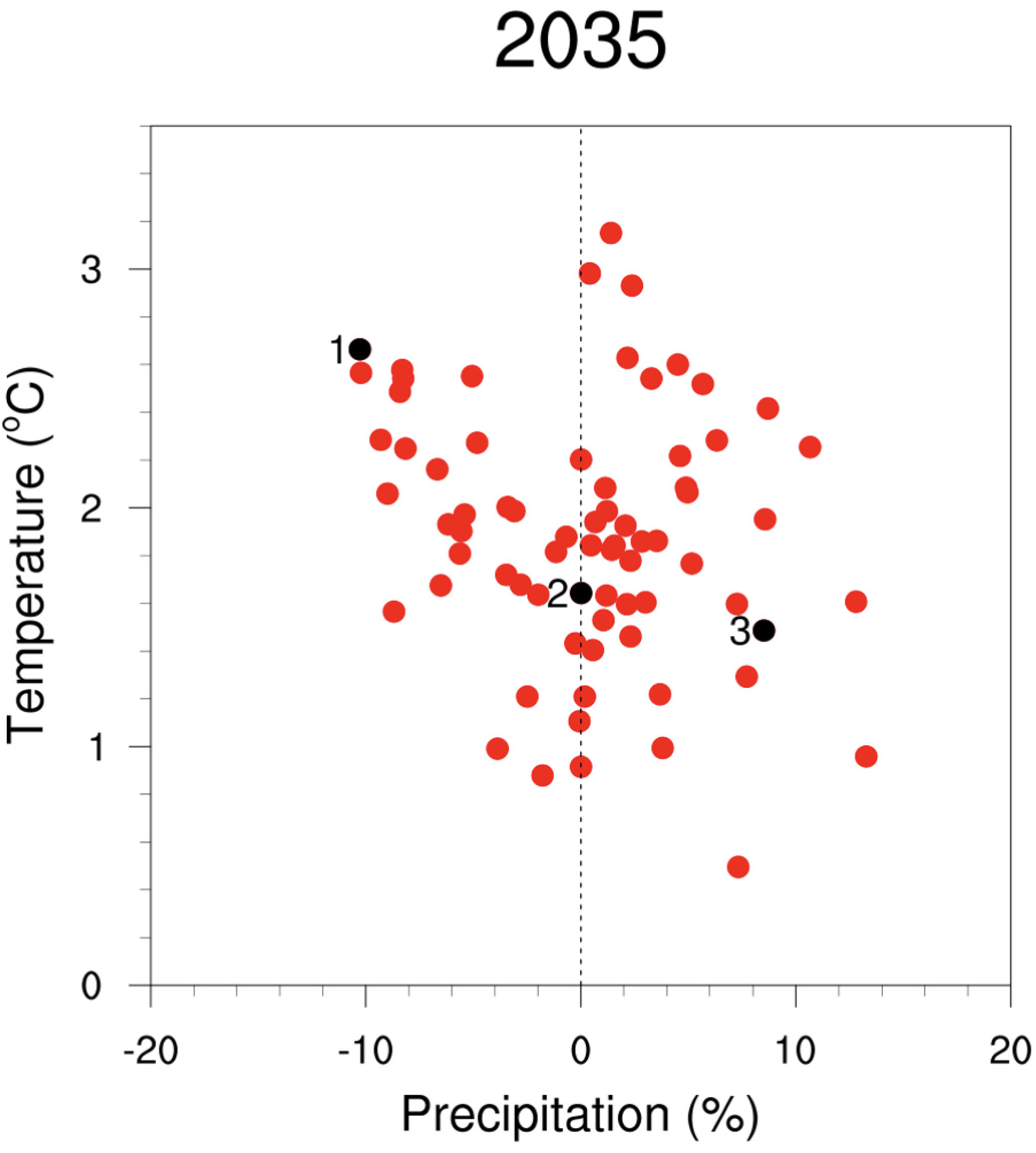
Southwest Colorado Social-Ecological Climate Resilience (SECR) Project: Pinyon-Juniper Landscape

The Southwest Colorado Social-Ecological Climate Resilience (SECR) Project utilized an interdisciplinary team of land managers, ecological and climate scientists, ranchers, and conservation planners to develop an innovative climate planning framework for four targeted landscapes. The Pinyon-Juniper landscape in the San Juan Basin described below was one of four landscapes evaluated throughout the 3-year duration of the SECR Project [17].
One of the management targets was the Pinyon-Juniper landscape. This 376,358-hectare landscape occurs on warm and dry foothills, mesas, canyons, and plateaus and consists of a mosaic of vegetation types; dominant tree species include pinyon pine (Pinus edulis), Utah juniper (Juniperus osteosperma), and Rocky Mountain juniper (J. scopulorum). Elevations are generally between 1,600–2,300 meters. The bi-modal precipitation pattern is important for cone crop production; winter precipitation primarily replenishes deep soil moisture, while summer precipitation provides shallow rooted plants with additional growing season moisture. Any change to the historic precipitation pattern is likely to influence mortality and recruitment of the dominant trees. These evergreen woodlands withstand very cold winter nights and hot summer days. The landscape is exceedingly rich with historic cultural resources, primarily from the ancestral Puebloans (500–1200 AD), as well as biological and land-use diversity. The assessment of ecological responses was evaluated using three climate scenarios: Hot and Dry, Feast or Famine and Warm and Wet to describe the potential future mid-century (2035) scenarios (described in Table S1 in Supplementary Materials).
Important climate metrics were compared across all three scenarios. Droughts similar to the 2002 severe drought year were projected to become more frequent (once every 5-years) in the Hot and Dry scenario compared to no change in drought frequency in the Warm and Wet scenario. The wildfire season was projected to increase in duration by 1- month per year in the Hot and Dry scenario, whereas, only a slight increase in the fire season was projected for the Warm and Wet scenario. The fire season was also projected to lengthen in the Feast or Famine scenario.
Both qualitative and quantitative ecological response models were developed. The important drivers were determined to be precipitation, temperature and drought. Winter moisture is critical for replenishing deep soil moisture and can help mitigate hot and dry summers. Summer monsoon moisture is required for pinyon pine cone production. Drought impacts are amplified by insects; Ips spp. bark beetles generally increase with drought and large old trees are more susceptible, leading to large die-off of mature trees. Fires are also more likely to increase in severity during severe droughts. Crown fires that kill the dominant pinyon and juniper trees are also more prevalent during drought years. For each climate scenario we delineated areas that were likely to be lost, threatened, persistent, and emergent for pinyon and juniper. Random Forest models were used to depict the change for each future scenario. Expert elicitation was used to evaluate the plausible socio-ecological impacts from the qualitative and quantitative response models. The process and plausible socio-ecological impacts are summarized below.
Climate 09 00177 i001

Appendix B

Case Study 2. Assessment of future southern white-tailed ptarmigan viability under three climate scenarios (Very Hot and Dry, Hot, and Hot and Very Wet; described in Table S2 in Supplementary Materials) using qualitative and quantitative ecological response models.
Species Status Assessment for the Southern White-tailed Ptarmigan (Ptarmigan SSA)

The U.S. Fish and Wildlife Service (USFWS) uses a species status assessment (SSA) framework to inform listing decisions under the Endangered Species Act (ESA; [165]). The SSA gathers available information on a species’ biology and ecological needs, assesses current conditions of the species’ habitats and populations, and forecasts future conditions for the species under a range of plausible scenarios. An SSA for the southern white-tailed ptarmigan (Lagopus leucura altipetens) was initiated in 2018 and involved an interdisciplinary collaboration of species experts, climate scientists, conservation geneticists, and population modelers. In 2020, the USFWS completed the SSA for the southern white-tailed ptarmigan [55], which was used to inform the determination that the subspecies was not warranted for listing.
The management target was the viability of the southern white-tailed ptarmigan. The subspecies inhabits alpine ecosystems at or above treeline year-round; in Colorado they occupy alpine habitats between 3353–4114 meters [166]. A conceptual model of habitat and demographic factors required by southern white-tailed ptarmigan to maintain population resiliency and support species viability was developed that included: (a) winter snow conditions that support well-distributed areas of soft snow suitable for snow roosting; (b) late-lying snowfields that help maintain brood-rearing habitats and provide thermal refugia; (c) summer precipitation/monsoonal moisture that provide regular cooling and late-season moisture; (d) brood-rearing habitat that provides young chicks with invertebrates and adults with chicks desirable forage forbs; and (e) abundant willow needed by all life stages that influences the distribution of ptarmigan.
Ptarmigan populations are maintained through immigration [167,168,169], emphasizing the importance of demographic connectivity among suitable alpine habitats.
The assessment of biological responses was evaluated using three climate scenarios: Very Hot and Dry, Hot, and Hot and Very Wet to describe the plausible future scenarios (described in Table S2 in Supplementary Materials) out to mid-century (2050). Several climate metrics important to ptarmigan habitat were considered under these scenarios, including frequency of severe drought, spring snowpack, seasonal temperatures, frequency of intense rainfall events, and monsoonal precipitation.
This SSA considered both qualitative and quantitative ecological response models. Expert input was used to evaluate the impacts of future climate scenarios on ptarmigan habitat and demography, specifically in terms of projections for temperature and precipitation. Dynamic global vegetation models (DGVMs) were also considered as a tool to inform the evaluation of future conditions for the southern white-tailed ptarmigan. However, the results of the DGVM that were evaluated conflicted with the understanding of the potential future habitat conditions for the southern white-tailed ptarmigan. Instead, the future condition of the southern white-tailed ptarmigan was evaluated under the three climate scenarios using several decades of demographic and ecological data in combination with expert input. The SSA process for the southern white-tailed ptarmigan and plausible impacts to habitat and demographic factors are summarized in the figure below.
Climate 09 00177 i002

References

  1. IPCC. Summary for Policymakers. In Climate Change 2021: The Physical Science Basis. Contribution of Working Group I to the Sixth Assessment Report of the Intergovernmental Panel on Climate Change; Masson-Delmotte, V., Zhai, P., Pirani, A., Connors, S.L., Péan, C., Berger, S., Caud, N., Chen, Y., Goldfarb, L., Gomis, M.I., et al., Eds.; Cambridge University Press: Cambridge, UK, 2021. [Google Scholar]
  2. Nolan, C.; Overpeck, J.T.; Allen, J.R.M.; Anderson, P.M.; Betancourt, J.L.; Binney, H.A.; Brewer, S.; Bush, M.B.; Chase, B.M.; Cheddadi, R. Past and future global transformation of terrestrial ecosystems under climate change. Science 2018, 361, 920–923. [Google Scholar] [CrossRef] [Green Version]
  3. Jackson, S.T. Transformational ecology and climate change. Science 2021, 373, 1085–1086. [Google Scholar] [CrossRef]
  4. Millar, C.I.; Stephenson, N.L. Temperate forest health in an era of emerging megadisturbance. Science 2015, 349, 823–826. [Google Scholar] [CrossRef]
  5. Díaz, S.; Settele, J.; Brondízio, E.S.; Ngo, H.T.; Agard, J.; Arneth, A.; Balvanera, P.; Brauman, K.A.; Butchart, S.H.M.; Chan, K.M.A. Pervasive human-driven decline of life on Earth points to the need for transformative change. Science 2019, 366, eaax3100. [Google Scholar] [CrossRef] [Green Version]
  6. Bridle, J.; van Rensburg, A. Discovering the limits of ecological resilience. Science 2020, 367, 626–627. [Google Scholar] [CrossRef] [PubMed]
  7. Crausbay, S.D.; Betancourt, J.; Bradford, J.; Cartwright, J.; Dennison, W.C.; Dunham, J.; Enquist, C.A.F.; Frazier, A.G.; Hall, K.R.; Littell, J.S. Unfamiliar territory: Emerging themes for ecological drought research and management. One Earth 2020, 3, 337–353. [Google Scholar] [CrossRef]
  8. Heino, J.; Alahuhta, J.; Bini, L.M.; Cai, Y.; Heiskanen, A.; Hellsten, S.; Kortelainen, P.; Kotamäki, N.; Tolonen, K.T.; Vihervaara, P. Lakes in the era of global change: Moving beyond single-lake thinking in maintaining biodiversity and ecosystem services. Biol. Rev. 2021, 96, 89–106. [Google Scholar] [CrossRef]
  9. Hughes, T.P.; Anderson, K.D.; Connolly, S.R.; Heron, S.F.; Kerry, J.T.; Lough, J.M.; Baird, A.H.; Baum, J.K.; Berumen, M.L.; Bridge, T.C. Spatial and temporal patterns of mass bleaching of corals in the Anthropocene. Science 2018, 359, 80–83. [Google Scholar] [CrossRef] [Green Version]
  10. Sully, S.; Burkepile, D.E.; Donovan, M.K.; Hodgson, G.; Van Woesik, R. A global analysis of coral bleaching over the past two decades. Nat. Commun. 2019, 10, 1264. [Google Scholar] [CrossRef] [Green Version]
  11. Grosse, G.; Goetz, S.; McGuire, A.D.; Romanovsky, V.E.; Schuur, E.A.G. Changing permafrost in a warming world and feedbacks to the Earth system. Environ. Res. Lett. 2016, 11, 40201. [Google Scholar] [CrossRef]
  12. Berner, L.T.; Massey, R.; Jantz, P.; Forbes, B.C.; Macias-Fauria, M.; Myers-Smith, I.; Kumpula, T.; Gauthier, G.; Andreu-Hayles, L.; Gaglioti, B.V. Summer warming explains widespread but not uniform greening in the Arctic tundra biome. Nat. Commun. 2020, 11, 4621. [Google Scholar] [CrossRef]
  13. Deutsch, C.A.; Tewksbury, J.J.; Tigchelaar, M.; Battisti, D.S.; Merrill, S.C.; Huey, R.B.; Naylor, R.L. Increase in crop losses to insect pests in a warming climate. Science 2018, 361, 916–919. [Google Scholar] [CrossRef] [PubMed] [Green Version]
  14. Nobre, C.A.; Sampaio, G.; Borma, L.S.; Castilla-Rubio, J.C.; Silva, J.S.; Cardoso, M. Land-use and climate change risks in the Amazon and the need of a novel sustainable development paradigm. Proc. Natl. Acad. Sci. USA 2016, 113, 10759–10768. [Google Scholar] [CrossRef] [Green Version]
  15. Macias-Fauria, M.; Post, E. Effects of sea ice on Arctic biota: An emerging crisis discipline. Biol. Lett. 2018, 14, 20170702. [Google Scholar] [CrossRef] [Green Version]
  16. Flynn, M.; Ford, J.D.; Pearce, T.; Harper, S.L.; Team, I.R. Participatory scenario planning and climate change impacts, adaptation and vulnerability research in the Arctic. Environ. Sci. Policy 2018, 79, 45–53. [Google Scholar] [CrossRef] [Green Version]
  17. Rondeau, R.; Bidwell, M.; Neely, B.; Rangwala, I.; Yung, L.; Wyborn, C. Pinyon-juniper landscape: San Juan Basin, Colorado Social-Ecological Climate Resilience Project Report. North Central Climate Science Center: Ft. Collins, CO, USA, 2017. Available online: https://www.sciencebase.gov/catalog/item/5d10f7e4e4b0941bde5502c4 (accessed on 10 September 2021).
  18. Symstad, A.J.; Fisichelli, N.A.; Miller, B.W.; Rowland, E.; Schuurman, G.W. Multiple methods for multiple futures: Integrating qualitative scenario planning and quantitative simulation modeling for natural resource decision making. Clim. Risk Manag. 2017, 17, 78–91. [Google Scholar] [CrossRef]
  19. Thorne, J.H.; Gogol-Prokurat, M.; Hill, S.; Walsh, D.; Boynton, R.M.; Choe, H. Vegetation refugia can inform climate-adaptive land management under global warming. Front. Ecol. Environ. 2020, 18, 281–287. [Google Scholar] [CrossRef]
  20. Raffini, F.; Bertorelle, G.; Biello, R.; D’Urso, G.; Russo, D.; Bosso, L. From nucleotides to satellite imagery: Approaches to identify and manage the invasive pathogen Xylella fastidiosa and its insect vectors in Europe. Sustainability 2020, 12, 4508. [Google Scholar] [CrossRef]
  21. Peterson, G.D.; Cumming, G.S.; Carpenter, S.R. Scenario planning: A tool for conservation in an uncertain world. Conserv. Biol. 2003, 17, 358–366. [Google Scholar] [CrossRef] [Green Version]
  22. Rowland, E.R.; Cross, M.S.; Hartmann, H. Considering Multiple Futures: Scenario Planning to Address Uncertainty in Natural Resource Conservation; Fish and Wildlife Service: Washington, DC, USA, 2014. [Google Scholar]
  23. Star, J.; Rowland, E.L.; Black, M.E.; Enquist, C.A.F.; Garfin, G.; Hoffman, C.H.; Hartmann, H.; Jacobs, K.L.; Moss, R.H.; Waple, A.M. Supporting adaptation decisions through scenario planning: Enabling the effective use of multiple methods. Clim. Risk Manag. 2016, 13, 88–94. [Google Scholar] [CrossRef] [Green Version]
  24. Ogden, A.E.; Innes, J.L. Application of structured decision making to an assessment of climate change vulnerabilities and adaptation options for sustainable forest management. Ecol. Soc. 2009, 14, 11. [Google Scholar] [CrossRef]
  25. Stein, B.A.; Glick, P.; Edelson, N.; Staudt, A. Climate-Smart Conservation: Putting Adaptation Principles into Practice [Online]; National Wildlife Federation: Washington, DC, USA, 2014. [Google Scholar]
  26. Cross, M.S.; Zavaleta, E.S.; Bachelet, D.; Brooks, M.L.; Enquist, C.A.F.; Fleishman, E.; Graumlich, L.J.; Groves, C.R.; Hannah, L.; Hansen, L. The Adaptation for Conservation Targets (ACT) framework: A tool for incorporating climate change into natural resource management. Environ. Manag. 2012, 50, 341–351. [Google Scholar] [CrossRef] [Green Version]
  27. Schuurman, G.W.; Hoffman, C.H.; Cole, D.N.; Lawrence, D.J.; Morton, J.M.; Magness, D.R.; Cravens, A.E.; Covington, S.; O’Malley, R.; Fisichelli, N.A. Resist-Accept-Direct (RAD)—A Framework for the 21st-Century Natural Resource Manager; Report no. NPS/NRSS/CCRP/NRR—2020/2213; National Park Service: Washington, DC, USA, 2020. [Google Scholar]
  28. Hausfather, Z.; Peters, G.P. Emissions—The ‘business as usual’story is misleading 2020. Nature 2020, 577, 618–620. [Google Scholar] [CrossRef]
  29. Burgess, M.G.; Ritchie, J.; Shapland, J.; Pielke, R. IPCC baseline scenarios have over-projected CO2 emissions and economic growth. Environ. Res. Lett. 2020, 16, 14016. [Google Scholar] [CrossRef]
  30. Held, H.; Aykut, S.; Hedemann, C.; Li, C.; Marotzke, J.; Petzold, J.; Schneider, U. Plausibility of model-based emissions scenarios. In Hamburg Climate Futures Outlook 2021: Assessing the Plausibility of Deep Decarbonization by 2050; Cluster of Excellence Climate, Climatic Change, and Society (CLICCS): Hamburg, Germany, 2021; pp. 21–26. [Google Scholar]
  31. Fowler, H.J.; Blenkinsop, S.; Tebaldi, C. Linking climate change modelling to impacts studies: Recent advances in downscaling techniques for hydrological modelling. Int. J. Climatol. A J. R. Meteorol. Soc. 2007, 27, 1547–1578. [Google Scholar] [CrossRef]
  32. Daniels, A.E.; Morrison, J.F.; Joyce, L.A.; Crookston, N.L.; Chen, S.-C.; McNulty, S.G. Climate Projections FAQ. In Gen. Tech. Rep. RMRS-GTR-277WWW; U.S. Department of Agriculture, Forest Service, Rocky Mountain Research Station: Fort Collins, CO, USA, 2012; Volume 277, 32 p. [Google Scholar]
  33. Kotamarthi, R.; Mearns, L.; Hayhoe, K.; Castro, C.L.; Wuebbles, D. Use of Climate Information for Decision-Making and Impacts Research: State of Our Understanding; Argonne National Laboratory: Lemont, IL, USA, 2016. [Google Scholar]
  34. Chakraborty, D.; Dobor, L.; Zolles, A.; Hlásny, T.; Schueler, S. High-resolution gridded climate data for Europe based on bias-corrected EURO-CORDEX: The ECLIPS dataset. Geosci. Data J. 2020, 8, 121–131. [Google Scholar] [CrossRef]
  35. Platts, P.J.; Omeny, P.; Marchant, R. AFRICLIM: High-resolution climate projections for ecological applications in Africa. Afr. J. Ecol. 2015, 53, 103–108. [Google Scholar] [CrossRef] [Green Version]
  36. Lukas, J.; Barsugli, J.; Doesken, N.; Rangwala, I.; Wolter, K. Climate change in Colorado: A synthesis to support water resources management and adaptation. Univ. Color. Boulder Color. 2014. [Google Scholar] [CrossRef]
  37. Roe, G.H.; Baker, M.B. Why is climate sensitivity so unpredictable? Science 2007, 318, 629–632. [Google Scholar] [CrossRef] [Green Version]
  38. Knutti, R. Should we believe model predictions of future climate change? Philos. Trans. R. Soc. A Math. Phys. Eng. Sci. 2008, 366, 4647–4664. [Google Scholar] [CrossRef] [PubMed]
  39. Hawkins, E.; Sutton, R. The potential to narrow uncertainty in regional climate predictions. Bull. Am. Meteorol. Soc. 2009, 90, 1095–1108. [Google Scholar] [CrossRef] [Green Version]
  40. Andrews, T.; Gregory, J.M.; Webb, M.J.; Taylor, K.E. Forcing, feedbacks and climate sensitivity in CMIP5 coupled atmosphere-ocean climate models. Geophys. Res. Lett. 2012, 39, L09712. [Google Scholar] [CrossRef] [Green Version]
  41. Vial, J.; Dufresne, J.-L.; Bony, S. On the interpretation of inter-model spread in CMIP5 climate sensitivity estimates. Clim. Dyn. 2013, 41, 3339–3362. [Google Scholar] [CrossRef]
  42. Ulbrich, U.; Leckebusch, G.C.; Pinto, J.G. Extra-tropical cyclones in the present and future climate: A review. Theor. Appl. Climatol. 2009, 96, 117–131. [Google Scholar] [CrossRef] [Green Version]
  43. Rangwala, I.; Pepin, N.; Vuille, M.; Miller, J. Influence of climate variability and large-scale circulation on the mountain cryosphere. In The High-Mountain Cryosphere: Environmental Changes and Human Risks; Cambridge University Press: Cambridge, UK, 2015; pp. 9–27. [Google Scholar]
  44. Kirtman, B.; Power, S.B.; Adedoyin, A.J.; Boer, G.J.; Bojariu, R.; Camilloni, I.; Doblas-Reyes, F.; Fiore, A.M.; Kimoto, M.; Meehl, G. Near-Term Climate Change: Projections and Predictability. In Climate Change 2013: The Physical Science Basis. Contribution of Working Group I to the Fifth Assessment Report of the Intergovernmental Panel on Climate Change; Stocker, T.F., Qin, D., Plattner, G.-K., Tignor, M., Allen, S.K., Boschung, J., Nauels, A., Xia, Y., Bex, V., Midgley, P.M., Eds.; Cambridge University Press: Cambridge, UK, 2013. [Google Scholar]
  45. Doblas-Reyes, F.J.; Sorensson, A.A.; Almazroui, M.; Dosio, A.; Gutowski, W.J.; Haarsma, R.; Hamdi, R.; Hewitson, B.; Kwon, W.-T.; Lamptey, B.L. Linking Global to Regional Climate Change. In Climate Change 2021: The Physical Science Basis. Contribution of Working Group I to the Sixth Assessment Report of the Intergovernmental Panel on Climate Change; Masson-Delmotte, V., Zhai, P., Pirani, A., Connors, S.L., Péan, C., Berger, S., Caud, N., Chen, Y., Goldfarb, L., Gomis, M.I., et al., Eds.; Cambridge University Press: Cambridge, UK, 2021. [Google Scholar]
  46. Lempert, R. Scenarios that illuminate vulnerabilities and robust responses. Clim. Chang. 2013, 117, 627–646. [Google Scholar] [CrossRef]
  47. Shepherd, T.G. Storyline approach to the construction of regional climate change information. Proc. R. Soc. A 2019, 475, 20190013. [Google Scholar] [CrossRef] [PubMed] [Green Version]
  48. Joyce, L.A.; Coulson, D. Climate scenarios and projections: A Technical Document Supporting the USDA Forest Service 2020 RPA Assessment. In Gen. Tech. Rep. RMRS-GTR-413; U.S. Department of Agriculture, Forest Service, Rocky Mountain Research Station: Fort Collins, CO, USA, 2020; Volume 413, 85p. [Google Scholar] [CrossRef]
  49. Lawrence, D.J.; Runyon, A.N.; Gross, J.E.; Schuurman, G.W.; Miller, B.W. Divergent, plausible, and relevant climate futures for near-and long-term resource planning. Clim. Chang. 2021, 167, 38. [Google Scholar] [CrossRef]
  50. Runyon, A.N.; Schuurman, G.W.; Miller, B.W.; Symstad, A.; Hardy, A. Climate Change Scenario Planning for Resource Stewardship at Wind Cave National Park; National Park Service: Ft. Collins, CO, USA, 2021. [Google Scholar]
  51. Weigel, A.P.; Knutti, R.; Liniger, M.A.; Appenzeller, C. Risks of model weighting in multimodel climate projections. J. Clim. 2010, 23, 4175–4191. [Google Scholar] [CrossRef]
  52. Mote, P.; Brekke, L.; Duffy, P.B.; Maurer, E. Guidelines for constructing climate scenarios. Eos. Trans. Am. Geophys. Union 2011, 92, 257–258. [Google Scholar] [CrossRef]
  53. Rupp, D.E.; Abatzoglou, J.T.; Hegewisch, K.C.; Mote, P.W. Evaluation of CMIP5 20th century climate simulations for the Pacific Northwest USA. J. Geophys. Res. Atmos. 2013, 118, 10–884. [Google Scholar] [CrossRef]
  54. Rupp, D.E. An Evaluation of 20th Century Climate for the Southeastern United States as Simulated by Coupled Model Intercomparison Project Phase 5 (CMIP5) Global Climate Models; U.S. Geological Survey Open-File Report 2016-1047; USGS: Raleigh, NC, USA, 2016; 32 p. [CrossRef] [Green Version]
  55. USFWS. Species Status Assessment Report for the Southern White-Tailed Ptarmigan (Lagopus leucura altipetens); US Fish and Wildlife Service: Lakewood, CO, USA, 2020. [Google Scholar]
  56. USFWS. Species Status Assessment Report for Colorado Hookless Cactus (Sclerocactus glaucus and Sclerocactus dawsonii); US Fish and Wildlife Service: Lakewood, CO, USA, 2021. [Google Scholar]
  57. Runyon, A.N.; Carlson, A.R.; Gross, J.; Lawrence, D.J.; Schuurman, G.W. Repeatable Approaches to Work with Scientific Uncertainty and Advance Climate Change Adaptation in US National Parks. Proc. Parks Steward. Forum 2020, 36. [Google Scholar] [CrossRef] [Green Version]
  58. Barsugli, J.J.; Guentchev, G.; Horton, R.M.; Wood, A.; Mearns, L.O.; Liang, X.; Winkler, J.A.; Dixon, K.; Hayhoe, K.; Rood, R.B. The practitioner’s dilemma: How to assess the credibility of downscaled climate projections. Eos. Trans. Am. Geophys. Union 2013, 94, 424–425. [Google Scholar] [CrossRef] [Green Version]
  59. Jennings, K.S.; Winchell, T.S.; Livneh, B.; Molotch, N.P. Spatial variation of the rain–snow temperature threshold across the Northern Hemisphere. Nat. Commun. 2018, 9, 1148. [Google Scholar] [CrossRef] [Green Version]
  60. Barsugli, J.J.; Ray, A.J.; Livneh, B.; Dewes, C.F.; Heldmyer, A.; Rangwala, I.; Guinotte, J.M.; Torbit, S. Projections of mountain snowpack loss for wolverine denning elevations in the Rocky Mountains. Earth’s Future 2020, 8, e2020EF001537. [Google Scholar] [CrossRef]
  61. Easterling, D.R.; Kunkel, K.E.; Arnold, J.R.; Knutson, T.; LeGrande, A.N.; Leung, L.R.; Vose, R.S.; Waliser, D.E.; Wehner, M.F. Precipitation Change in the United States BT-Climate Science Special Report: Fourth National Climate Assessment; Wuebbles, D.J., Fahey, D.W., Hibbard, K.A., Dokken, D.J., Stewart, B.C., Maycock, T.K., Eds.; U.S. Global Change Research Program: Washington, DC, USA, 2017; pp. 207–230.
  62. Kendon, E.J.; Roberts, N.M.; Senior, C.A.; Roberts, M.J. Realism of rainfall in a very high-resolution regional climate model. J. Clim. 2012, 25, 5791–5806. [Google Scholar] [CrossRef]
  63. Chan, S.C.; Kendon, E.J.; Roberts, N.M.; Fowler, H.J.; Blenkinsop, S. The characteristics of summer sub-hourly rainfall over the southern UK in a high-resolution convective permitting model. Environ. Res. Lett. 2016, 11, 94024. [Google Scholar] [CrossRef]
  64. Liu, C.; Ikeda, K.; Rasmussen, R.; Barlage, M.; Newman, A.J.; Prein, A.F.; Chen, F.; Chen, L.; Clark, M.; Dai, A. Continental-scale convection-permitting modeling of the current and future climate of North America. Clim. Dyn. 2017, 49, 71–95. [Google Scholar] [CrossRef]
  65. Fowler, H.J.; Lenderink, G.; Prein, A.F.; Westra, S.; Allan, R.P.; Ban, N.; Barbero, R.; Berg, P.; Blenkinsop, S.; Do, H.X. Anthropogenic intensification of short-duration rainfall extremes. Nat. Rev. Earth Environ. 2021, 2, 107–122. [Google Scholar] [CrossRef]
  66. Redmond, K.T. The depiction of drought: A commentary. Bull. Am. Meteorol. Soc. 2002, 83, 1143–1147. [Google Scholar] [CrossRef] [Green Version]
  67. Hobbins, M.; Rangwala, I.; Barsugli, J.; Dewes, C. Extremes in evaporative demand and their implications for droughts and drought monitoring in the 21st century. In Extreme Hydrology and Climate Variability; Elsevier: Amsterdam, The Netherlands, 2019; pp. 325–341. [Google Scholar]
  68. Ficklin, D.L.; Novick, K.A. Historic and projected changes in vapor pressure deficit suggest a continental-scale drying of the United States atmosphere. J. Geophys. Res. Atmos. 2017, 122, 2061–2079. [Google Scholar] [CrossRef]
  69. Williams, A.P.; Allen, C.D.; Macalady, A.K.; Griffin, D.; Woodhouse, C.A.; Meko, D.M.; Swetnam, T.W.; Rauscher, S.A.; Seager, R.; Grissino-Mayer, H.D. Temperature as a potent driver of regional forest drought stress and tree mortality. Nat. Clim. Chang. 2013, 3, 292–297. [Google Scholar] [CrossRef]
  70. Urban, M.C.; Bocedi, G.; Hendry, A.P.; Mihoub, J.-B.; Pe’er, G.; Singer, A.; Bridle, J.R.; Crozier, L.G.; De Meester, L.; Godsoe, W. Improving the forecast for biodiversity under climate change. Science 2016, 353, aad8466. [Google Scholar] [CrossRef] [Green Version]
  71. Tewksbury, J.J.; Anderson, J.G.T.; Bakker, J.D.; Billo, T.J.; Dunwiddie, P.W.; Groom, M.J.; Hampton, S.E.; Herman, S.G.; Levey, D.J.; Machnicki, N.J. Natural history’s place in science and society. Bioscience 2014, 64, 300–310. [Google Scholar] [CrossRef] [Green Version]
  72. Dawson, T.P.; Jackson, S.T.; House, J.I.; Prentice, I.C.; Mace, G.M. Beyond predictions: Biodiversity conservation in a changing climate. Science 2011, 332, 53–58. [Google Scholar] [CrossRef] [PubMed] [Green Version]
  73. Lepetz, V.; Massot, M.; Schmeller, D.S.; Clobert, J. Biodiversity monitoring: Some proposals to adequately study species’ responses to climate change. Biodivers. Conserv. 2009, 18, 3185–3203. [Google Scholar] [CrossRef]
  74. Pacifici, M.; Foden, W.B.; Visconti, P.; Watson, J.E.M.; Butchart, S.H.M.; Kovacs, K.M.; Scheffers, B.R.; Hole, D.G.; Martin, T.G.; Akçakaya, H.R. Assessing species vulnerability to climate change. Nat. Clim. Chang. 2015, 5, 215–224. [Google Scholar] [CrossRef]
  75. Buckley, L.B. Linking traits to energetics and population dynamics to predict lizard ranges in changing environments. Am. Nat. 2008, 171, E1–E19. [Google Scholar] [CrossRef] [Green Version]
  76. Coops, N.C.; Waring, R.H.; Schroeder, T.A. Combining a generic process-based productivity model and a statistical classification method to predict the presence and absence of tree species in the Pacific Northwest, USA. Ecol. Modell. 2009, 220, 1787–1796. [Google Scholar] [CrossRef]
  77. Angilletta, M.J., Jr.; Angilletta, M.J. Thermal Adaptation: A Theoretical and Empirical Synthesis; Oxford University Press: Oxford, UK, 2009. [Google Scholar] [CrossRef]
  78. Fisichelli, N.; Wright, A.; Rice, K.; Mau, A.; Buschena, C.; Reich, P.B. First-year seedlings and climate change: Species-specific responses of 15 North American tree species. Oikos 2014, 123, 1331–1340. [Google Scholar] [CrossRef]
  79. Chapin III, F.S.; Shaver, G.R. Physiological and growth responses of arctic plants to a field experiment simulating climatic change. Ecology 1996, 77, 822–840. [Google Scholar] [CrossRef]
  80. Liu, H.; Mi, Z.; Lin, L.I.; Wang, Y.; Zhang, Z.; Zhang, F.; Wang, H.; Liu, L.; Zhu, B.; Cao, G. Shifting plant species composition in response to climate change stabilizes grassland primary production. Proc. Natl. Acad. Sci. USA 2018, 115, 4051–4056. [Google Scholar] [CrossRef] [Green Version]
  81. Stewart, R.I.A.; Dossena, M.; Bohan, D.A.; Jeppesen, E.; Kordas, R.L.; Ledger, M.E.; Meerhoff, M.; Moss, B.; Mulder, C.; Shurin, J.B. Mesocosm experiments as a tool for ecological climate-change research. Adv. Ecol. Res. 2013, 48, 71–181. [Google Scholar]
  82. Henry, G.H.R.; Molau, U. Tundra plants and climate change: The International Tundra Experiment (ITEX). Glob. Chang. Biol. 1997, 3, 1–9. [Google Scholar] [CrossRef]
  83. Fraser, L.H.; Henry, H.A.L.; Carlyle, C.N.; White, S.R.; Beierkuhnlein, C.; Cahill, J.F., Jr.; Casper, B.B.; Cleland, E.; Collins, S.L.; Dukes, J.S. Coordinated distributed experiments: An emerging tool for testing global hypotheses in ecology and environmental science. Front. Ecol. Environ. 2013, 11, 147–155. [Google Scholar] [CrossRef] [Green Version]
  84. Guisan, A.; Thuiller, W. Predicting species distribution: Offering more than simple habitat models. Ecol. Lett. 2005, 8, 993–1009. [Google Scholar] [CrossRef] [PubMed]
  85. Mouquet, N.; Lagadeuc, Y.; Devictor, V.; Doyen, L.; Duputié, A.; Eveillard, D.; Faure, D.; Garnier, E.; Gimenez, O.; Huneman, P. Predictive ecology in a changing world. J. Appl. Ecol. 2015, 52, 1293–1310. [Google Scholar] [CrossRef]
  86. Wadgymar, S.M.; Ogilvie, J.E.; Inouye, D.W.; Weis, A.E.; Anderson, J.T. Phenological responses to multiple environmental drivers under climate change: Insights from a long-term observational study and a manipulative field experiment. New Phytol. 2018, 218, 517–529. [Google Scholar] [CrossRef] [Green Version]
  87. Nogués-Bravo, D.; Rodríguez-Sánchez, F.; Orsini, L.; de Boer, E.; Jansson, R.; Morlon, H.; Fordham, D.A.; Jackson, S.T. Cracking the code of biodiversity responses to past climate change. Trends Ecol. Evol. 2018, 33, 765–776. [Google Scholar] [CrossRef] [Green Version]
  88. Fordham, D.A.; Jackson, S.T.; Brown, S.C.; Huntley, B.; Brook, B.W.; Dahl-Jensen, D.; Gilbert, M.T.P.; Otto-Bliesner, B.L.; Svensson, A.; Theodoridis, S. Using paleo-archives to safeguard biodiversity under climate change. Science 2020, 369, eabc5654. [Google Scholar] [CrossRef]
  89. Case, M.J.; Lawler, J.J.; Tomasevic, J.A. Relative sensitivity to climate change of species in northwestern North America. Biol. Conserv. 2015, 187, 127–133. [Google Scholar] [CrossRef]
  90. Martin, T.G.; Burgman, M.A.; Fidler, F.; Kuhnert, P.M.; Low-Choy, S.; McBride, M.; Mengersen, K. Eliciting expert knowledge in conservation science. Conserv. Biol. 2012, 26, 29–38. [Google Scholar] [CrossRef] [Green Version]
  91. Nabhan, G.P. Perspectives in Ethnobiology: Ethnophenology and climate change. J. Ethnobiol. 2010, 30, 1–4. [Google Scholar] [CrossRef]
  92. Vinyeta, K.; Lynn, K. Exploring the role of traditional ecological knowledge in climate change initiatives. In Gen. Tech. Rep. PNW-GTR-879; U.S. Department of Agriculture, Forest Service, Pacific Northwest Research Station: Portland, OR, USA, 2013; Volume 879, 37 p. [Google Scholar]
  93. Smith, S.D.P.; Bunnell, D.B.; Burton, G.A., Jr.; Ciborowski, J.J.H.; Davidson, A.D.; Dickinson, C.E.; Eaton, L.A.; Esselman, P.C.; Evans, M.A.; Kashian, D.R. Evidence for interactions among environmental stressors in the Laurentian Great Lakes. Ecol. Indic. 2019, 101, 203–211. [Google Scholar] [CrossRef]
  94. Krivtsov, V. Investigations of indirect relationships in ecology and environmental sciences: A review and the implications for comparative theoretical ecosystem analysis. Ecol. Modell. 2004, 174, 37–54. [Google Scholar] [CrossRef]
  95. Tylianakis, J.M.; Didham, R.K.; Bascompte, J.; Wardle, D.A. Global change and species interactions in terrestrial ecosystems. Ecol. Lett. 2008, 11, 1351–1363. [Google Scholar] [CrossRef]
  96. Suttle, K.B.; Thomsen, M.A.; Power, M.E. Species interactions reverse grassland responses to changing climate. Science 2007, 315, 640–642. [Google Scholar] [CrossRef] [Green Version]
  97. Santini, L.; Cornulier, T.; Bullock, J.M.; Palmer, S.C.F.; White, S.M.; Hodgson, J.A.; Bocedi, G.; Travis, J.M.J. A trait-based approach for predicting species responses to environmental change from sparse data: How well might terrestrial mammals track climate change? Glob. Chang. Biol. 2016, 22, 2415–2424. [Google Scholar] [CrossRef] [Green Version]
  98. Bozinovic, F.; Pörtner, H. Physiological ecology meets climate change. Ecol. Evol. 2015, 5, 1025–1030. [Google Scholar] [CrossRef] [PubMed]
  99. Knapp, A.K.; Hoover, D.L.; Wilcox, K.R.; Avolio, M.L.; Koerner, S.E.; La Pierre, K.J.; Loik, M.E.; Luo, Y.; Sala, O.E.; Smith, M.D. Characterizing differences in precipitation regimes of extreme wet and dry years: Implications for climate change experiments. Glob. Chang. Biol. 2015, 21, 2624–2633. [Google Scholar] [CrossRef] [Green Version]
  100. Pearson, R.G.; Dawson, T.P. Predicting the impacts of climate change on the distribution of species: Are bioclimate envelope models useful? Glob. Ecol. Biogeogr. 2003, 12, 361–371. [Google Scholar] [CrossRef] [Green Version]
  101. Ummenhofer, C.C.; Meehl, G.A. Extreme weather and climate events with ecological relevance: A review. Philos. Trans. R. Soc. B Biol. Sci. 2017, 372, 20160135. [Google Scholar] [CrossRef]
  102. Garcia, R.A.; Cabeza, M.; Rahbek, C.; Araújo, M.B. Multiple dimensions of climate change and their implications for biodiversity. Science 2014, 344, 1247579. [Google Scholar] [CrossRef] [Green Version]
  103. Helmuth, B.; Russell, B.D.; Connell, S.D.; Dong, Y.; Harley, C.D.G.; Lima, F.P.; Sará, G.; Williams, G.A.; Mieszkowska, N. Beyond long-term averages: Making biological sense of a rapidly changing world. Clim. Chang. Responses 2014, 1, 1–13. [Google Scholar] [CrossRef] [Green Version]
  104. Navarro, M.Á.P.; Sapes, G.; Batllori, E.; Serra-Diaz, J.M.; Esteve, M.A.; Lloret, F. Climatic suitability derived from species distribution models captures community responses to an extreme drought episode. Ecosystems 2019, 22, 77–90. [Google Scholar] [CrossRef] [Green Version]
  105. Germain, S.J.; Lutz, J.A. Climate extremes may be more important than climate means when predicting species range shifts. Clim. Chang. 2020, 163, 579–598. [Google Scholar] [CrossRef]
  106. Cuena-Lombraña, A.; Fois, M.; Fenu, G.; Cogoni, D.; Bacchetta, G. The impact of climatic variations on the reproductive success of Gentiana lutea L. in a Mediterranean mountain area. Int. J. Biometeorol. 2018, 62, 1283–1295. [Google Scholar] [CrossRef] [PubMed]
  107. Jentsch, A.; Beierkuhnlein, C. Research frontiers in climate change: Effects of extreme meteorological events on ecosystems. Comptes Rendus Geosci. 2008, 340, 621–628. [Google Scholar] [CrossRef]
  108. Wethey, D.S.; Woodin, S.A.; Hilbish, T.J.; Jones, S.J.; Lima, F.P.; Brannock, P.M. Response of intertidal populations to climate: Effects of extreme events versus long term change. J. Exp. Mar. Bio. Ecol. 2011, 400, 132–144. [Google Scholar] [CrossRef]
  109. Harris, R.M.B.; Beaumont, L.J.; Vance, T.R.; Tozer, C.R.; Remenyi, T.A.; Perkins-Kirkpatrick, S.E.; Mitchell, P.J.; Nicotra, A.B.; McGregor, S.; Andrew, N.R. Biological responses to the press and pulse of climate trends and extreme events. Nat. Clim. Chang. 2018, 8, 579–587. [Google Scholar] [CrossRef]
  110. Maxwell, S.L.; Butt, N.; Maron, M.; McAlpine, C.A.; Chapman, S.; Ullmann, A.; Segan, D.B.; Watson, J.E.M. Conservation implications of ecological responses to extreme weather and climate events. Divers. Distrib. 2019, 25, 613–625. [Google Scholar] [CrossRef]
  111. Weiskopf, S.R.; Rubenstein, M.A.; Crozier, L.G.; Gaichas, S.; Griffis, R.; Halofsky, J.E.; Hyde, K.J.W.; Morelli, T.L.; Morisette, J.T.; Muñoz, R.C. Climate change effects on biodiversity, ecosystems, ecosystem services, and natural resource management in the United States. Sci. Total Environ. 2020, 733, 137782. [Google Scholar] [CrossRef]
  112. Turner, M.G.; Calder, W.J.; Cumming, G.S.; Hughes, T.P.; Jentsch, A.; LaDeau, S.L.; Lenton, T.M.; Shuman, B.N.; Turetsky, M.R.; Ratajczak, Z. Climate change, ecosystems and abrupt change: Science priorities. Philos. Trans. R. Soc. B 2020, 375, 20190105. [Google Scholar] [CrossRef] [Green Version]
  113. Batllori, E.; Lloret, F.; Aakala, T.; Anderegg, W.R.L.; Aynekulu, E.; Bendixsen, D.P.; Bentouati, A.; Bigler, C.; Burk, C.J.; Camarero, J.J. Forest and woodland replacement patterns following drought-related mortality. Proc. Natl. Acad. Sci. USA 2020, 117, 29720–29729. [Google Scholar] [CrossRef] [PubMed]
  114. Sofaer, H.R.; Barsugli, J.J.; Jarnevich, C.S.; Abatzoglou, J.T.; Talbert, M.K.; Miller, B.W.; Morisette, J.T. Designing ecological climate change impact assessments to reflect key climatic drivers. Glob. Chang. Biol. 2017, 23, 2537–2553. [Google Scholar] [CrossRef] [PubMed]
  115. Albano, C.M.; McCarthy, M.I.; Dettinger, M.D.; McAfee, S.A. Techniques for constructing climate scenarios for stress test applications. Clim. Chang. 2021, 164, 1–25. [Google Scholar] [CrossRef]
  116. Williams, J.W.; Jackson, S.T. Novel climates, no-analog communities, and ecological surprises. Front. Ecol. Environ. 2007, 5, 475–482. [Google Scholar] [CrossRef]
  117. Van de Pol, M.; Jenouvrier, S.; Cornelissen, J.H.C.; Visser, M.E. Behavioural, ecological and evolutionary responses to extreme climatic events: Challenges and directions. Phil. Trans. R. Soc. B 2017, 372, 20160134. [Google Scholar] [CrossRef] [PubMed] [Green Version]
  118. Smith, M.D. An ecological perspective on extreme climatic events: A synthetic definition and framework to guide future research. J. Ecol. 2011, 99, 656–663. [Google Scholar] [CrossRef]
  119. Kayler, Z.E.; De Boeck, H.J.; Fatichi, S.; Grünzweig, J.M.; Merbold, L.; Beier, C.; McDowell, N.; Dukes, J.S. Experiments to confront the environmental extremes of climate change. Front. Ecol. Environ. 2015, 13, 219–225. [Google Scholar] [CrossRef]
  120. Fuentes, M.; Maynard, J.A.; Guinea, M.; Bell, I.P.; Werdell, P.J.; Hamann, M. Proxy indicators of sand temperature help project impacts of global warming on sea turtles in northern Australia. Endanger. Species Res. 2009, 9, 33–40. [Google Scholar] [CrossRef] [Green Version]
  121. Mair, L.; Jönsson, M.; Räty, M.; Bärring, L.; Strandberg, G.; Lämås, T.; Snäll, T. Land use changes could modify future negative effects of climate change on old-growth forest indicator species. Divers. Distrib. 2018, 24, 1416–1425. [Google Scholar] [CrossRef] [Green Version]
  122. Moraitis, M.L.; Valavanis, V.D.; Karakassis, I. Modelling the effects of climate change on the distribution of benthic indicator species in the Eastern Mediterranean Sea. Sci. Total Environ. 2019, 667, 16–24. [Google Scholar] [CrossRef] [PubMed]
  123. Cramer, W.; Bondeau, A.; Woodward, F.I.; Prentice, I.C.; Betts, R.A.; Brovkin, V.; Cox, P.M.; Fisher, V.; Foley, J.A.; Friend, A.D. Global response of terrestrial ecosystem structure and function to CO2 and climate change: Results from six dynamic global vegetation models. Glob. Chang. Biol. 2001, 7, 357–373. [Google Scholar] [CrossRef] [Green Version]
  124. Daniel, C.J.; Frid, L.; Sleeter, B.M.; Fortin, M. State-and-transition simulation models: A framework for forecasting landscape change. Methods Ecol. Evol. 2016, 7, 1413–1423. [Google Scholar] [CrossRef] [Green Version]
  125. Hijmans, R.J.; Graham, C.H. The ability of climate envelope models to predict the effect of climate change on species distributions. Glob. Chang. Biol. 2006, 12, 2272–2281. [Google Scholar] [CrossRef]
  126. Elith, J.; Leathwick, J.R. Species distribution models: Ecological explanation and prediction across space and time. Annu. Rev. Ecol. Evol. Syst. 2009, 40, 677–697. [Google Scholar] [CrossRef]
  127. Jenouvrier, S.; Caswell, H.; Barbraud, C.; Holland, M.; Strœve, J.; Weimerskirch, H. Demographic models and IPCC climate projections predict the decline of an emperor penguin population. Proc. Natl. Acad. Sci. USA 2009, 106, 1844–1847. [Google Scholar] [CrossRef] [Green Version]
  128. Morgan, M.G.; Pitelka, L.F.; Shevliakova, E. Elicitation of expert judgments of climate change impacts on forest ecosystems. Clim. Chang. 2001, 49, 279–307. [Google Scholar] [CrossRef]
  129. O’Neill, S.J.; Osborn, T.J.; Hulme, M.; Lorenzoni, I.; Watkinson, A.R. Using expert knowledge to assess uncertainties in future polar bear populations under climate change. J. Appl. Ecol. 2008, 45, 1649–1659. [Google Scholar] [CrossRef]
  130. Herr, A.; Dambacher, J.M.; Pinkard, E.; Glen, M.; Mohammed, C.; Wardlaw, T. The uncertain impact of climate change on forest ecosystems–How qualitative modelling can guide future research for quantitative model development. Environ. Model. Softw. 2016, 76, 95–107. [Google Scholar] [CrossRef]
  131. Weeks, D.; Malone, P.; Welling, L. Climate change scenario planning: A tool for managing parks into uncertain futures. Park Sci. 2011, 28, 26–33. [Google Scholar]
  132. Beeton, T.A.; McNeeley, S.M.; Miller, B.W.; Ojima, D.S. Grounding simulation models with qualitative case studies: Toward a holistic framework to make climate science usable for US public land management. Clim. Risk Manag. 2019, 23, 50–66. [Google Scholar] [CrossRef]
  133. Marcot, B.G.; Holthausen, R.S.; Raphael, M.G.; Rowland, M.M.; Wisdom, M.J. Using Bayesian belief networks to evaluate fish and wildlife population viability under land management alternatives from an environmental impact statement. For. Ecol. Manage. 2001, 153, 29–42. [Google Scholar] [CrossRef]
  134. Bode, M.; Baker, C.M.; Benshemesh, J.; Burnard, T.; Rumpff, L.; Hauser, C.E.; Lahoz-Monfort, J.J.; Wintle, B.A. Revealing beliefs: Using ensemble ecosystem modelling to extrapolate expert beliefs to novel ecological scenarios. Methods Ecol. Evol. 2017, 8, 1012–1021. [Google Scholar] [CrossRef] [Green Version]
  135. Miller, B.W.; Symstad, A.J.; Frid, L.; Fisichelli, N.A.; Schuurman, G.W. Co-producing simulation models to inform resource management: A case study from southwest South Dakota. Ecosphere 2017, 8, e02020. [Google Scholar] [CrossRef] [Green Version]
  136. Austin, M.P.; Van Niel, K.P. Improving species distribution models for climate change studies: Variable selection and scale. J. Biogeogr. 2011, 38, 1–8. [Google Scholar] [CrossRef]
  137. Franklin, J.; Davis, F.W.; Ikegami, M.; Syphard, A.D.; Flint, L.E.; Flint, A.L.; Hannah, L. Modeling plant species distributions under future climates: How fine scale do climate projections need to be? Glob. Chang. Biol. 2013, 19, 473–483. [Google Scholar] [CrossRef] [Green Version]
  138. Beaumont, L.J.; Hughes, L.; Pitman, A.J. Why is the choice of future climate scenarios for species distribution modelling important? Ecol. Lett. 2008, 11, 1135–1146. [Google Scholar] [CrossRef]
  139. Urban, M.C.; Tewksbury, J.J.; Sheldon, K.S. On a collision course: Competition and dispersal differences create no-analogue communities and cause extinctions during climate change. Proc. R. Soc. B Biol. Sci. 2012, 279, 2072–2080. [Google Scholar] [CrossRef] [PubMed] [Green Version]
  140. Lavergne, S.; Mouquet, N.; Thuiller, W.; Ronce, O. Biodiversity and climate change: Integrating evolutionary and ecological responses of species and communities. Annu. Rev. Ecol. Evol. Syst. 2010, 41, 321–350. [Google Scholar] [CrossRef] [Green Version]
  141. Ockendon, N.; Baker, D.J.; Carr, J.A.; White, E.C.; Almond, R.E.A.; Amano, T.; Bertram, E.; Bradbury, R.B.; Bradley, C.; Butchart, S.H.M. Mechanisms underpinning climatic impacts on natural populations: Altered species interactions are more important than direct effects. Glob. Chang. Biol. 2014, 20, 2221–2229. [Google Scholar] [CrossRef] [PubMed]
  142. D’Amen, M.; Rahbek, C.; Zimmermann, N.E.; Guisan, A. Spatial predictions at the community level: From current approaches to future frameworks. Biol. Rev. 2017, 92, 169–187. [Google Scholar] [CrossRef] [PubMed]
  143. Heikkinen, R.K.; Luoto, M.; Virkkala, R.; Pearson, R.G.; Körber, J. Biotic interactions improve prediction of boreal bird distributions at macro-scales. Glob. Ecol. Biogeogr. 2007, 16, 754–763. [Google Scholar] [CrossRef]
  144. Davis, A.J.; Jenkinson, L.S.; Lawton, J.H.; Shorrocks, B.; Wood, S. Making mistakes when predicting shifts in species range in response to global warming. Nature 1998, 391, 783–786. [Google Scholar] [CrossRef]
  145. Thomas, C.D.; Cameron, A.; Green, R.E.; Bakkenes, M.; Beaumont, L.J.; Collingham, Y.C.; Erasmus, B.F.N.; De Siqueira, M.F.; Grainger, A.; Hannah, L. Extinction risk from climate change. Nature 2004, 427, 145–148. [Google Scholar] [CrossRef]
  146. Buma, B. Disturbance interactions: Characterization, prediction, and the potential for cascading effects. Ecosphere 2015, 6, 1–15. [Google Scholar] [CrossRef]
  147. Yates, K.L.; Bouchet, P.J.; Caley, M.J.; Mengersen, K.; Randin, C.F.; Parnell, S.; Fielding, A.H.; Bamford, A.J.; Ban, S.; Barbosa, A.M. Outstanding challenges in the transferability of ecological models. Trends Ecol. Evol. 2018, 33, 790–802. [Google Scholar] [CrossRef] [PubMed] [Green Version]
  148. Burkett, V.R.; Wilcox, D.A.; Stottlemyer, R.; Barrow, W.; Fagre, D.; Baron, J.; Price, J.; Nielsen, J.L.; Allen, C.D.; Peterson, D.L. Nonlinear dynamics in ecosystem response to climatic change: Case studies and policy implications. Ecol. Complex. 2005, 2, 357–394. [Google Scholar] [CrossRef] [Green Version]
  149. Perret, D.L.; Leslie, A.B.; Sax, D.F. Naturalized distributions show that climatic disequilibrium is structured by niche size in pines (Pinus L.). Glob. Ecol. Biogeogr. 2019, 28, 429–441. [Google Scholar] [CrossRef]
  150. Bonan, G.B.; Doney, S.C. Climate, ecosystems, and planetary futures: The challenge to predict life in Earth system models. Science 2018, 359, 6375. [Google Scholar] [CrossRef] [PubMed] [Green Version]
  151. Alexander, J.M.; Chalmandrier, L.; Lenoir, J.; Burgess, T.I.; Essl, F.; Haider, S.; Kueffer, C.; McDougall, K.; Milbau, A.; Nuñez, M.A. Lags in the response of mountain plant communities to climate change. Glob. Chang. Biol. 2018, 24, 563–579. [Google Scholar] [CrossRef]
  152. Bertrand, R.; Lenoir, J.; Piedallu, C.; Riofrio-Dillon, G.; de Ruffray, P.; Vidal, C.; Pierrat, J.-C.; Gégout, J.-C. Changes in plant community composition lag behind climate warming in lowland forests. Nature 2011, 479, 517–520. [Google Scholar] [CrossRef]
  153. Svenning, J.; Sandel, B. Disequilibrium vegetation dynamics under future climate change. Am. J. Bot. 2013, 100, 1266–1286. [Google Scholar] [CrossRef]
  154. McLaughlin, B.C.; Zavaleta, E.S. Predicting species responses to climate change: Demography and climate microrefugia in C alifornia valley oak (Quercus lobata). Glob. Chang. Biol. 2012, 18, 2301–2312. [Google Scholar] [CrossRef]
  155. Williams, J.W.; Ordonez, A.; Svenning, J.-C. A unifying framework for studying and managing climate-driven rates of ecological change. Nat. Ecol. Evol. 2021, 5, 17–26. [Google Scholar] [CrossRef]
  156. Comte, L.; Grenouillet, G. Do stream fish track climate change? Assessing distribution shifts in recent decades. Ecography 2013, 36, 1236–1246. [Google Scholar]
  157. Bachelet, D.; Ferschweiler, K.; Sheehan, T.J.; Sleeter, B.M.; Zhu, Z. Projected carbon stocks in the conterminous USA with land use and variable fire regimes. Glob. Chang. Biol. 2015, 21, 4548–4560. [Google Scholar] [CrossRef] [PubMed]
  158. Slavich, E.; Warton, D.I.; Ashcroft, M.B.; Gollan, J.R.; Ramp, D. Topoclimate versus macroclimate: How does climate mapping methodology affect species distribution models and climate change projections? Divers. Distrib. 2014, 20, 952–963. [Google Scholar] [CrossRef]
  159. Dullinger, S.; Dirnböck, T.; Grabherr, G. Modelling climate change-driven treeline shifts: Relative effects of temperature increase, dispersal and invasibility. J. Ecol. 2004, 92, 241–252. [Google Scholar] [CrossRef]
  160. Harsch, M.A.; Bader, M.Y. Treeline form–A potential key to understanding treeline dynamics. Glob. Ecol. Biogeogr. 2011, 20, 582–596. [Google Scholar] [CrossRef]
  161. Rondeau, R.; Fink, M.; Rodda, G.; Kummel, M. Treeline Monitoring in the San Juan Basin Tundra: A Pilot Project. Ph.D. Thesis, Colorado State University, Fort Collins, CO, USA, 2012. [Google Scholar]
  162. Fink, M.; Rondeau, R.; Decker, K. Treeline Monitoring in the San Juan Mountains; Unpublished Report, Colorado Natural Heritage Program; Colorado State University: Ft. Collins, CO, USA, 2014; Available online: https://cnhp.colostate.edu/wp-content/uploads/download/documents/2014/Final_Treeline_report_2014.pdf (accessed on 10 September 2021).
  163. Davis, E.L.; Brown, R.; Daniels, L.; Kavanagh, T.; Gedalof, Z. Regional variability in the response of alpine treelines to climate change. Clim. Chang. 2020, 162, 1365–1384. [Google Scholar] [CrossRef]
  164. Miller, B.W.; Morisette, J.T. Integrating research tools to support the management of social-ecological systems under climate change. Ecol. Soc. 2014, 19, 1–12. [Google Scholar] [CrossRef] [Green Version]
  165. Smith, D.R.; Allan, N.L.; McGowan, C.P.; Szymanski, J.A.; Oetker, S.R.; Bell, H.M. Development of a species status assessment process for decisions under the US Endangered Species Act. J. Fish Wildl. Manag. 2018, 9, 302–320. [Google Scholar] [CrossRef] [Green Version]
  166. Seglund, A.; Street, P.A.; Aagaard, K.; Runge, J.; Flenner, M. Southern White-Tailed Ptarmigan (Lagopus leucura altipetens) Population Assessment and Conservation Considerations in Colorado, Unpublished Report; Colorado Parks and Wildlife: Denver, CO, USA, 2018.
  167. Martin, K.; Stacey, P.B.; Braun, C.E. Recruitment, dispersal, and demographic rescue in spatially-structured white-tailed ptarmigan populations. Condor 2000, 102, 503–516. [Google Scholar] [CrossRef]
  168. Sandercock, B.K.; Martin, K.; Hannon, S.J. Life history strategies in extreme environments: Comparative demography of arctic and alpine ptarmigan. Ecology 2005, 86, 2176–2186. [Google Scholar] [CrossRef]
  169. Wann, G.T. Reproductive Ecology and Population Viability of Alpine-Endemic Ptarmigan Populations in Colorado. Ph.D. Thesis, Colorado State University, Fort Collins, CO, USA, 2017. [Google Scholar]
Figure 1. Process flow diagram of a typical approach for conducting biological impact assessments under different future climate scenarios. The curved arrows demonstrate the iterative (i.e., non-linear) process of integrating climate and ecology methods in conservation projects (e.g., Case Study 1 and 2 in Appendix A).
Climate 09 00177 g001
Figure 2. Bivariate–scatter plots show changes in annual temperature and precipitation by three different future time horizons–2035 (2020–2049), 2050 (2035–2064) and 2070 (2055–2084)–from 72 global climate model (GCM) projections for the southwest Colorado region (36.5–41° N, 102–109° W) as described in [17] (see also Case Study 1 in Appendix A). All changes are relative to 1971–2000. Each circle represents changes between the averages of future and historical periods for a single GCM projection. Red and blue circles indicate changes under high (RCP 8.5) and medium (RCP 4.5) greenhouse gas emission scenarios with each point representing a projection from a different global climate model. The scatter for changes in temperature between RCP 8.5 and RCP 4.5 is similar by 2035; high overlap by 2050 with the range in RCP 8.5 about 1 °C warmer than RCP 4.5; very little overlap by 2070 with the range in RCP 8.5 more than 2 °C warmer than RCP 4.5. On the other hand, the scatter for changes in precipitation between RCP 8.5 and RCP 4.5 remains similar at all future time horizons. For regional scale climate change, uncertainty associated with future greenhouse gas emission scenarios only becomes important after the mid-century time horizon for temperature and temperature-induced effects and much less so for precipitation changes across different emission scenarios.
Climate 09 00177 g002
Figure 3. Temperature change projected for the Colorado Front Range by 2035–2065 (relative to 1985–2015) from 21 Global Climate Models (GCMs) under RCP 8.5 compared to GCMs’ climate sensitivity. The Colorado Front Range considered here is the region between 37.2° N–41° N and 104.85° W–106.6° W. Regional temperature change is strongly related to the model’s climate sensitivity. Climate sensitivity data is obtained from [40,41]; temperature data is obtained from US Reclamation’s Downscaled CMIP5 Climate Projections (see Table 2).
Climate 09 00177 g003
Figure 4. Projections from two different datasets quantifying changes in annual temperature and precipitation by 2050 (2035–2064 relative to 1971–2000) for the central US Great Plains (32–46° N, 92–105° W) for the same greenhouse gas (GHG) emission scenario (RCP 8.5) are compared. Thirty–five distinct global climate model (GCM) projections indicated by Red circles (where each projection is from a different GCM; CMIP5–35) are compared to 30 projections from a single model (CESM1–30) indicated by Blue circles. The scatter from CMIP5–35 suggests a temperature change of 1.5 °C–4 °C, and a precipitation change of –10% to +10% (although most of the projections show increases in future precipitation). The scatter from CESM1–30 suggests a temperature change of 2.8 °C–3.6 °C and a precipitation change of 0% to +10%. The difference in projections in CESM1–30 can all be attributed to natural variability. The comparison of the two datasets implies that precipitation projections are significantly influenced by natural variability, which can explain 50% or more of the future variation in precipitation. Temperature projections are also influenced by natural variability, but to a smaller degree (~30%).
Climate 09 00177 g004
Figure 5. Three plausible and divergent climate scenarios for the southwest Colorado region were selected to inform the Social Ecological and Climate Resiliency (SECR) project (see also Case Study 1 in Appendix A). Red circles show changes in annual temperature and precipitation by the 2035 (2020–2049) time horizon under both a high (RCP 8.5) and a medium (RCP 4.5) greenhouse gas emission scenario. Black circles are the three selected scenarios, that were, respectively, named as: (1) Hot and Dry, (2) Feast or Famine and (3) Warm and Wet, to incorporate the divergence in future climate projections uncertainty into the assessment of future ecological responses.
Climate 09 00177 g005
Table 1. Sources of uncertainty, complexity and constraints encountered in assessing the impacts of climate change on ecosystems and species; GHG and GCMs refer to greenhouse gas and Global Climate Models, respectively.
ClimateEcology
Uncertainty
Differences in projected climate change or ecological impacts arising from differences across climate models, emission scenarios, and choice and structure of ecological methods and models
  • GHG Emission Scenarios, important particularly after 2050
  • Projections across GCMs
    Regional temperature change is strongly affected by differences across GCMs
    Regional precipitation change is strongly affected by natural variability
  • Differences across different downscaling methods. Even greater differences across hydrological model projections that are driven by downscaled climate projections, to obtain high spatial resolution information on metrics like snow, soil moisture and runoff
  • Differences in projected response across ecological models
  • Uncertainty arising from climate parameters incorporated into ecological models
  • Uncertainty arising from underlying population/ecosystem dynamics simulated in the model
  • Uncertainty arising from how demographic processes are related to variation in climate in models
Complexity
Complex interactions between climate and ecological process and their relevant spatiotemporal scales
  • Influence of stochasticity (including short-term extreme events) and sequencing of climate events
  • Sensitivities of species or ecosystem to different climate metrics
  • Stochasticity in ecological processes (e.g., demographic stochasticity, contingencies in community assembly, etc.)
  • Lags between species distributions and climate suitability
  • Interactions and/or feedbacks among multiple disturbances, ecosystem processes, and species
Constraints
Availability of suitable observed and modeled data at appropriate spatiotemporal scales
  • Availability of ecologically-sensitive hydroclimate variables at appropriate spatio-temporal scales
    Snow, soil moisture, streamflow, extreme precipitation, monsoon, winds, freeze-thaw cycle, frost risk, storms
  • Downscaled climate projections (1–10 km) are still pretty coarse to inform changes across the landscape at management-relevant scales (e.g., identifying climate refugia)
  • Lack of long-term ecological datasets with sufficient variation in climate
  • Difficulty integrating population dynamics into projected changes in habitat availability
  • Lack of information about likely extreme events, and difficulty including extremes in ecological models
  • Limitations of models in terms of spatial scale, model complexity, expertise, or computational ability
Table 2. List of web tools to create bivariate-scatter plots of climate projections for a given location and time horizon, and access downscaled spatial and time-series data for select climate scenarios.
ToolFeaturesWebsite
Climate Toolbox
  • Scenario selection (bivariate scatter plots)
  • Time series data and spatial data layers for individual projection
  • Various derived climate variables including extreme climate metrics
  • Several plotting routines to perform analysis
  • Observed data
  • Region selection: Rectangular region & point location within CONUS
  • Easy to use
  • Emission scenarios: RCP 4.5, 8.5
  • Downscaled Climate data: MACAv2-METDATA
https://climatetoolbox.org/
USGS National Climate Change Viewer
  • Scenario selection (bivariate scatter plots)
  • Time series data for ensemble projection
  • Climate and hydrology metrics
  • Region selection: States and Counties in CONUS
  • Assessment of model agreement
  • Easy to use
  • Emission scenarios: RCP 4.5, 8.5
  • Downscaled Climate data: MACAv2-METDATA
https://www2.usgs.gov/landresources/lcs/nccv/maca2/maca2_counties.html
US Reclamation’s Downscaled CMIP3 and CMIP5 Climate Projections
  • Time series data and spatial data layers for individual projection
  • Climate and hydrology metrics
  • Region selection: Rectangular region & pre-defined large watersheds within CONUS
  • Primarily data extraction and limited analysis capabilities
  • Emission scenarios: RCP 2.6, 4.5, 6.0, 8.5
  • Downscaled Climate data: BCSD, LOCA, BCCA
https://gdo-dcp.ucllnl.org/
KNMI Climate Explorer
  • Time series data and spatial data layers for individual projection
  • Climate and hydrology metrics
  • Region selection: Global
  • Both data extraction and analysis capabilities
  • Monthly CMIP5 and CMIP6 data
  • Original GCM Data
  • Moderately difficult to use
https://climexp.knmi.nl/start.cgi
Climate Futures Toolbox
  • Extraction of spatial data layers for individual projection
  • Region selection: Shapefiles within CONUS
  • User need knowledge of R
  • Emission scenarios: RCP 4.5, 8.5
  • Downscaled Climate data: MACAv2-METDATA
https://www.earthdatascience.org/cft/index.html
WorldClim
  • Extraction of very high resolution spatial data layers selected future periods (20-year averages) and projections
  • Region selection: Global
  • CMIP6 data
  • Downscaled Climate data: BCSD
  • Easy to use
https://www.worldclim.org/data/cmip6/cmip6climate.html
Publisher’s Note: MDPI stays neutral with regard to jurisdictional claims in published maps and institutional affiliations.

