
Lorenz Atmospheric Energy Cycle in Climatic Projections


Climate and Atmosphere Research Centre (CARE-C), The Cyprus Institute, 2121 Nicosia, Cyprus
Climate 2021, 9(12), 180; https://0-doi-org.brum.beds.ac.uk/10.3390/cli9120180
Submission received: 14 November 2021
/
Revised: 3 December 2021
/
Accepted: 7 December 2021
/
Published: 10 December 2021
(This article belongs to the Section Climate Dynamics and Modelling)
Abstract
:The aim of this study is to investigate whether different Representative Concentration Pathways (RCPs), as they are determined in the Fifth Assessment Report (AR5) of the Intergovernmental Panel on Climate Change (IPCC), lead to different regimes in the energetics components of the Lorenz energy cycle. The four energy forms on which this investigation is based are the zonal and eddy components of the available potential and kinetic energies. The corresponding transformations between these forms of energy are also studied. RCPs are time-dependent, consistent scenarios of concentrations of radiatively active gases and particles. In the present study, four RCPs are explored, namely, rcp26, rcp45, rcp60, rcp85; these represent projections (for the future period 2006–2100) that result in radiative forcing of approximately 2.6, 4.5, 6.0 and 8.5 Wm−2 at year 2100, respectively, relative to pre-industrial conditions. The results are presented in terms of time projections of the energetics components from 2020 to 2100 and show that the different RCPs yield diverse energetics regimes, consequently impacting the Lorenz energy cycle. In this respect, projections under different RCPs of the Lorenz energy cycle are presented.
1. Introduction
The study of the energetics of the atmosphere comprises a fundamental approach in the efforts to understand the dynamics of the Earth’s atmosphere. Since the 1950s, the energetics of the atmosphere have attracted the interest of several investigations (e.g., [1,2,3]). The focus of such studies is on the fate of the available potential energy and kinetic energy.
The formulation of the concept of available potential energy by Lorenz was built upon Margules’s [4] concept founded on a hypothetical adiabatic redistribution of the atmospheric mass. The concept has been widely exploited in studies of general circulation and large-scale dynamics [5]. Although the original concept was formulated almost 120 years ago, it has undergone a number of further refinements and reformulations (e.g., [6,7]). The concept is still under examination from different perspectives (e.g., [8,9]).
Lorenz [10,11] considered that from the sum of potential and internal energies, which he termed total potential energy, only a part is available for conversion into kinetic energy, as a result of an adiabatic redistribution of the mass of the atmosphere; this part of the total potential energy is what he called available potential energy. Basically, as determined by Lorenz, the energy cycle describes the fate of these forms of atmospheric energy, namely, the available potential energy and kinetic energy, through energy conversion. In addition, in this energy cycle, available potential energy is generated by diabatic processes and kinetic energy is dissipated by friction.
Lorenz proceeded further into expanding the above energy cycle into a more refined one by contemplating the eddy character of the atmospheric flow, in an effort to identify which atmospheric motions are primarily responsible for the energy conversion. In this respect, he partitioned each of the available potential energy and kinetic energy into zonal and eddy components.
Following the publication of Lorenz’s aspects on the fate of atmospheric energy, a number of studies have been carried out in search of estimates of the various energy cycle components. Oort [1] performed a critical survey of estimates of various energetics components obtained previously by several investigators for the large-scale generation, dissipation, and conversion of energy in the atmosphere. From a comparative study of these previously fragmented findings, he made a selection, which “in the author’s opinion, were representative for the yearly energy cycle in the Northern Hemisphere” and appraised a quantified energy cycle. In his landmark monograph “The nature and theory of the general circulation of the atmosphere”, Lorenz [10] endorsed Oort’s first estimates of the energy cycle, but he concurrently postulated that these would not be the final word. Subsequent studies on the energy cycle were hampered by the lack of suitable data at appropriate spatiotemporal resolutions (see [3]). For example, Krueger et al. [12] performed computations of the energy cycle for a five-year period, using data based on objectively analyzed contour heights of the 850 and 500 hPa surfaces and vertical velocities that were obtained from a baroclinic model. For their computations, Dutton and Johnson [13] used the daily isentropic cross sections for 1958 along 75°W from the north to south poles and together with previously but partly established estimations, they produced new estimates of the complete energy cycle. Wiin-Nielsen [14] performed computations of components of the energy cycle for a period of one year in an effort to establish their annual variation. A fairly more complete description of the annual cycle of the energetics of the entire northern hemisphere is given by Oort and Peixóto [15] who made use of upper air analyses based on 600 radiosonde stations over a five-years period.
With the advent of initialized analyses of meteorological variables, the study of the atmospheric energy cycle turned into these consistent and spatiotemporally more detailed databases. Oriol [16] performed a one-year energy budget computation with data from the European Centre for Medium Range Forecasts (ECMWF). Kung and Tanaka [17], who made use of data from the First Global Atmospheric Research Program (GARP), reached new estimates for the energy cycle, which differed from previous estimates; they attributed this discrepancy to an earlier restriction in the availability of data. They have also noted notable differences between estimates made with different datasets. Using data from the ECMWF analyses, Ullbrich and Speth [18] studied the global energy cycle for the months of January and June in a seven-year period.
The availability of the reanalysis data gave a new dimension to the study of atmospheric energetics; therefore, recently, there has been a rather limited number of studies that make use of long-term global data in order to study changes in the Lorenz energy cycle, which are referred to herein. In the first study by Hu et al. [19], variations of the northern hemisphere energetics during the period 1948–2000 are reported. By splitting this period into two epochs (1948–1978 and 1979–2000), they generated estimates of the energy cycle for these two epochs and noted important differences between them, which they found to be season-independent. In the second study by Marques et al. [20], data for the period 1979–2001 retrieved from the Reanalysis-2 dataset of NCEP (National Centres for Environmental Prediction) [21] and from the ERA40 reanalysis by ECMWF [22] were employed. From the energetics point of view, their computations with the two datasets did not reveal appreciable differences. Atmospheric energetics were also computed using ECMWF Reanalyses for the period 1958–1978. A significant increase was found in the eddy kinetic and eddy available potential energies from the early period to the later period, which the authors attributed to the assimilation in the reanalyses of satellite data after 1979.
Unsurprisingly, the availability of data on future climate scenarios widens the research prospects for new studies of the energy cycle. Increasing greenhouse gas concentrations imply an increase in global mean temperature, but the way that this may affect the energetics of the atmosphere and the underlying physical processes is not straightforward; hence, further investigation on this issue is required. The motivation for such an approach is that any long-term changes in the Lorenz energy cycle could have important climatic implications that are not adequately addressed otherwise.
As elaborated above, the Lorenz energy cycle is founded upon two principal forms of energy, namely, the available potential and kinetic energies; the cycle involves physical atmospheric processes leading to the generation of available potential energy and dissipation of kinetic energy, as well as conversions between energy forms. When viewed within the framework of this energy cycle, the climate system may be contemplated as a heat engine in which thermodynamic energy is converted into kinetic energy, which is ultimately dissipated into heat. The overall strength of the energy cycle gives a “rate of working” of the climate system [23].
The present study has been carried out within the context of different greenhouse gas concentrations, as they are implicated in future climate change scenarios. In this respect, the effect of these climatic scenarios on the Lorenz energy cycle is examined from a long-term perspective.
The World Climate Research Programmes’ (WCRP) Coupled Model Intercomparison Project (CMIP) is a collaborative scientific effort aiming at improving knowledge of climate change. CMIP—Phase 5 (CMIP5) is a completed phase of this project, addressing unresolved scientific questions regarding its outputs that are useful to those considering possible consequences of climate change. A detailed description of the CMIP5 experiment design is provided by Taylor et al. [24]. Within this framework, a family of Representative Concentration Pathways (RCPs) scenarios has been established [25]. RCPs identify the value of the additional radiative forcing (due to the anthropic contribution), expressed in W/m2, expected for the year 2100 (compared to the pre-industrial year 1750). These RCPs are subsequently used as input to several experiments with the adoption of global models of the climate system, thus generating a multi-model dataset designed to advance our knowledge of climate, its variability and change.
The objective of the present study is to investigate whether different Representative Concentration Pathways (RCPs) lead to different regimes in the energetics components of the Lorenz energy cycle, which would therefore have an impact on a “rate of working” of the climate system.
The available scientific literature on the topics of the present study is very limited. Boer and Lambert [23] computed the energy cycle components of twelve climatic models participating in the Second Phase of the Atmospheric Model Intercomparison Project (AMIP2 [26]), intercompared them and assessed the results against observational calculations based on reanalyses by NCEP [21] and ERA [22] (ECMWF Re-Analysis). Their study focused on the period from 1979 to 1995 and compiled model results into “ensemble model results”, which the authors suggest that they perform better than individual model results in the comparison of energy cycle quantities with reanalysis-based values.
Hernández-Deckers and von Storch [27] evaluated the Lorenz energy cycle responses to CO2 increases, using output from the atmosphere–ocean ECHAM5/Max Planck Institute Ocean Model (MPI-OM). Their study found that doubling of CO2 results in a decrease in the energy cycle strength, in terms of the total conversion of available potential energy into kinetic energy and also in an increase in the zonal kinetic energy. They also related these global changes to a strengthening of the energy cycle in the upper troposphere and a weakening below; these opposite responses resulted from the simulated warming pattern exhibiting the strongest warming in the upper tropical troposphere and in the lower troposphere at high latitudes. This warming structure subsequently led to changes in the horizontal temperature variance and in mean static stability, increasing the zonal available potential energy in the upper troposphere and decreasing it below, which triggers the two opposite responses via changes in baroclinicity.
Veiga and Ambrizzi [28] used a set of projections originating from the Max Planck Institute Earth System Model (MPI-ESM) that was also used in CMIP5 in order to study the effect of different RCPs on the Lorenz energy cycle. Their research applied the same approach to the global atmosphere but also to the two Earth’s hemispheres, which were treated separately. The period which the research of Veiga and Ambrizzi [28] refers to is from 2005 to 2100, which is somewhat longer than the one used in the present study.
Following this introduction, Section 2 describes the data that have been used and the methodology adopted. The results are presented in Section 3: Section 3.1 presents the energy balance and Section 3.2 the time series and trends of the energetics components under different RCP-based scenarios. Section 4 comprises the discussion part that includes some future plans.
2. Materials and Methods
The calculations of the energetics components and their corresponding dynamical processes, as they are implicated in the numerical solution of the mathematical expressions describing the Lorenz energy cycle components, which present by themselves great computational challenges. These calculations call for the estimation of horizontal and vertical derivatives, as well as vertical integrations and area averaging. Limitations imposed on the vertical derivatives and integrals by the lower and upper atmospheric boundaries, as well as on the derivatives and area averages imposed by the singularities at the poles are a few of such challenges requiring special computational handling.
2.1. Data
In this study, the output from the HadGEM2-ES model has been utilized. HadGEM2-ES is an Earth System model adopted by the British Meteorological Office Hadley Centre for the CMIP5 centennial simulations [29]. This climate model includes a coupled ocean-atmosphere configuration, the terrestrial and ocean carbon cycle and tropospheric chemistry. Details on HadGEM2-ES are given by Collins et al. [30] and Martin et al. [31].
The output from the HadGEM2-ES model forms the basis for this work, which focuses on the daily calculation of the various components of the Lorenz energy cycle [10,32] for the period covered by the dataset, namely, from 2015 till 2100; however, in the present paper, results for the period from 2020 till the end of this century under different RCPs are presented. The results presented in the following refer to the global atmosphere.
Four RCPs have been employed in the study: one high pathway for which radiative forcing reaches >8.5 Wm−2 by year 2100 and continues to rise for some amount of time (termed as rcp85); two intermediate “stabilization pathways” in which radiative forcing is stabilized at approximately 6 Wm−2 and 4.5 Wm−2 after year 2100, (rcp60 and rcp45, respectively); one pathway where radiative forcing peaks at approximately 2.6 Wm−2 before year 2100, declining afterward (rcp26).
The present study is based on climate projections in the period from 2020 to 2100 (i.e., 80 years), resulting from the CMIP5 experiments with the HadGEM2-ES model. The experiments embrace different ensembles of the model setup, which facilitate the quantification of the variability of the simulation data concerning the model. In this respect, ensemble members are characterized by specific realizations, initialization methods and physics. The r1i1p1 ensemble is used herein (where, the prefixes “r”, “i” and “p” denote the number of realizations, and the initialization and physics methods, respectively).
The climatic projections used are daily gridded fields of temperature (T), eastward and northward wind components (u and v, respectively) and Lagrangian pressure tendency (or vertical velocity, ω) available at a 2.5° × 1.875° (lat-lon) spatial resolution and at eight isobaric levels, namely, 1000, 850, 700, 500, 250, 100, 50 and 10 hPa. A daily time resolution is employed and each year in the database is considered to have 360 days. Hence, the total number of days involved in the calculation of the energetics is 80 × 360 = 28,800, for each RCP. The best estimates of the energy cycle have been obtained by using the particular set of data available within the CMIP5 project.
2.2. Formulation of the Problem
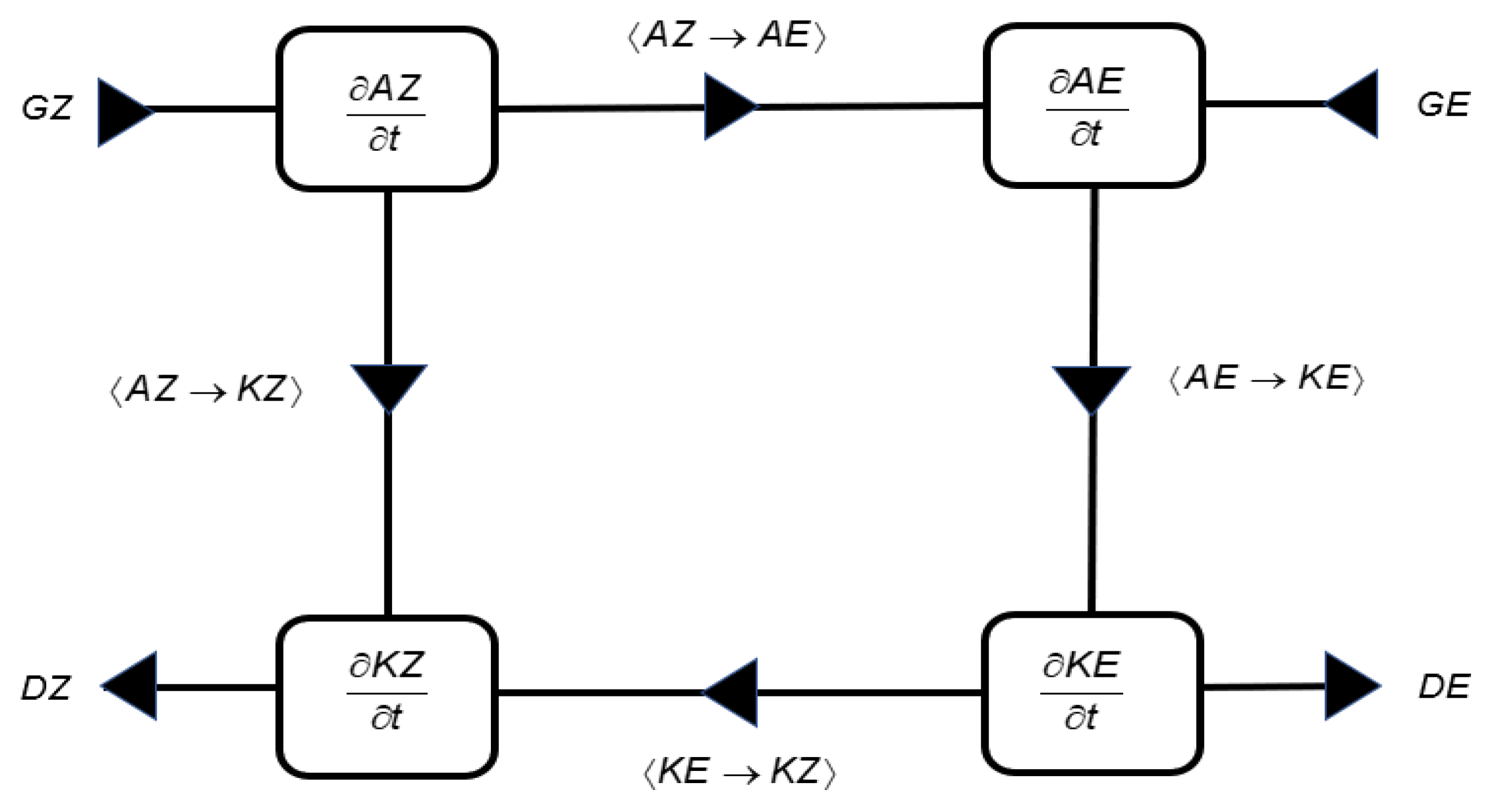
Bearing the above in mind, the four energy forms involved in this energy cycle are shown in Figure 1: zonal and eddy available potential energies (hereafter denoted by AZ and AE, respectively), on the one hand, and zonal and eddy kinetic energies (hereafter denoted by KZ and KE, respectively), on the other hand; the rates of change of these energy forms are shown in the boxes as local derivatives with respect to time (t). In order to comply with Lorenz’s conceptualization of the mean direction of flow of energy on the global scale, the arrows in this figure denote positively valued conversions. For any two forms of energy, e.g., X and Y, the symbolic representation of energy conversions, e.g., <X→Y>, implies conversion from X into Y for positive values and reversed conversion for negative values; therefore, <Y→X> = − <X→Y>.
The process that converts available potential energy into kinetic energy is described as a sinking of colder air and rising of warmer air. This is resolved into two sub-processes. The first is described as the sinking of colder air in colder latitude zones and rising of warmer air in warmer latitude zones, denoted by <AZ→KZ>. The second is described as the sinking of colder air and rising of warmer air at the same latitude, denoted by <AE→KE>.
Observational investigations have long shown that the transport of angular momentum by eddies is predominantly toward zones of higher angular velocity (e.g., westerly jet-streams), so that KE is converted into KZ by the eddies themselves. This is denoted by the conversion term <KE→KZ>.
A process that can convert AZ into AE (without altering the total available potential energy) is a horizontal or vertical transport by the eddies of sensible heat toward zones where the temperature is low, relative to the horizontally averaged temperature. This is denoted by <AZ→AE>.
The diabatic generation terms of zonal and eddy available potential energies are considered as positive inputs to the respective available potential energy rates. Generation of AZ (denoted by GZ) is accomplished through diabatic heating at lower latitudes and cooling at higher latitudes, whereas heating of warmer regions and cooling of colder ones at the same latitude generates AE (denoted by GE).
The dissipation of zonal and eddy kinetic energies, denoted by DZ and DE, respectively, are considered as negative inputs (or sinks), i.e., contributing to the direction of reducing the respective kinetic energy rates. For the dissipation of KZ and KE, the processes are the zonally averaged frictional processes and the deviation of friction from its zonal average, respectively.
2.3. Methodology
The convention adopted here allows for the formulation of a set of differential equations describing the Lorenz energy cycle (see Equations (1)–(4)). In each of these four equations, the term on the left-hand side represents the local rate of change of one of the energy forms and the right-hand side consists of three positive or negative inputs, as follows:
All the energy quantities, rates of change and conversions are numerically calculated; having calculated the rates of change and the conversion terms, the generation and dissipation terms are estimated as residuals in the respective differential equations.
The original formulation of the available potential energy concept by Lorenz [11] was developed by considering averages and variances of pressure on isentropic surfaces. Lorenz [11] has also shown how the mathematical expressions for available potential energy, kinetic energy, energy conversions, available potential energy generation and dissipation of kinetic energy can be expressed in terms of variables defined on isobaric surfaces. These mathematical expressions are volume integrals of quite complex functions of temperature, wind velocity components and vertical velocity. Muench [33,34] has presented a detailed derivation of appropriate expressions for the energy integrals in which the variables used are functions of latitude, longitude and isobaric pressure level. The mathematical formulations by Muench [33,34] are suitable for the computation of the energy cycle components presented herein, bearing in mind that the variables generated by the HadGEM2-ES model and made available to CMIP5 are given as functions of latitude, longitude and pressure level. Indeed, for each of the 28,800 days in every RCP, the fields of velocity, temperature and Lagrangian pressure tendency are resolved at eight pressure levels on a 144 × 192 (lat-lon) grid.
The numerical solution of the integrals requires the employment of appropriate numerical techniques (see [35,36,37]). In Appendix A, the numerical analogs of the terms on the right-hand side of Equations (1)–(4) are given, together with the numerical techniques adopted herein for the numerical calculation of the energy components. As it is also shown in Appendix A, the necessity to handle non-numerical values in the original set of data and the need for formulating appropriate numerical techniques for the computation of the mathematical formulations of the energetics components is quite challenging.
3. Results
To demonstrate that different RCP-based scenarios yield diverse energetics regimes, consequently impacting the Lorenz energy cycle and the efficiency with which atmospheric energy is generated, converted and dissipated, the results of the study are given in two forms: firstly, as energy balances, and secondly, as time series of the energetics components.
3.1. Energy Balance
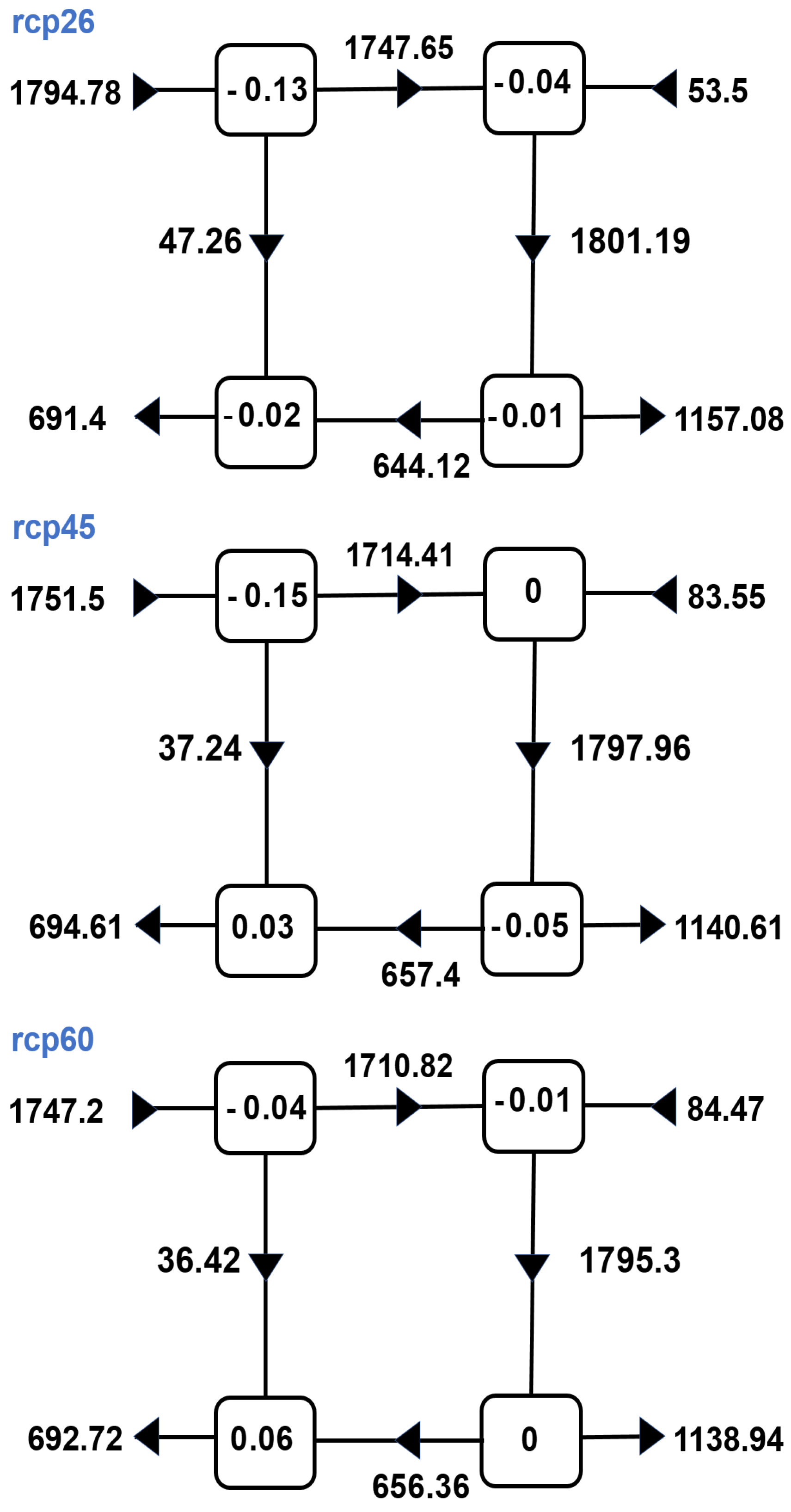
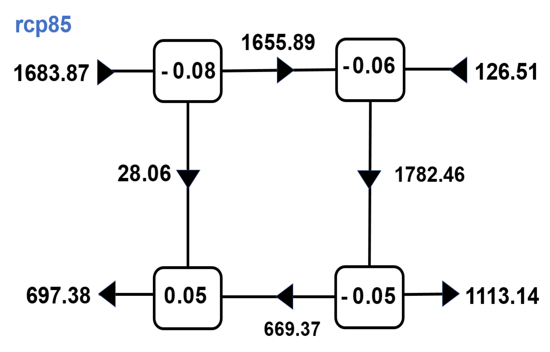
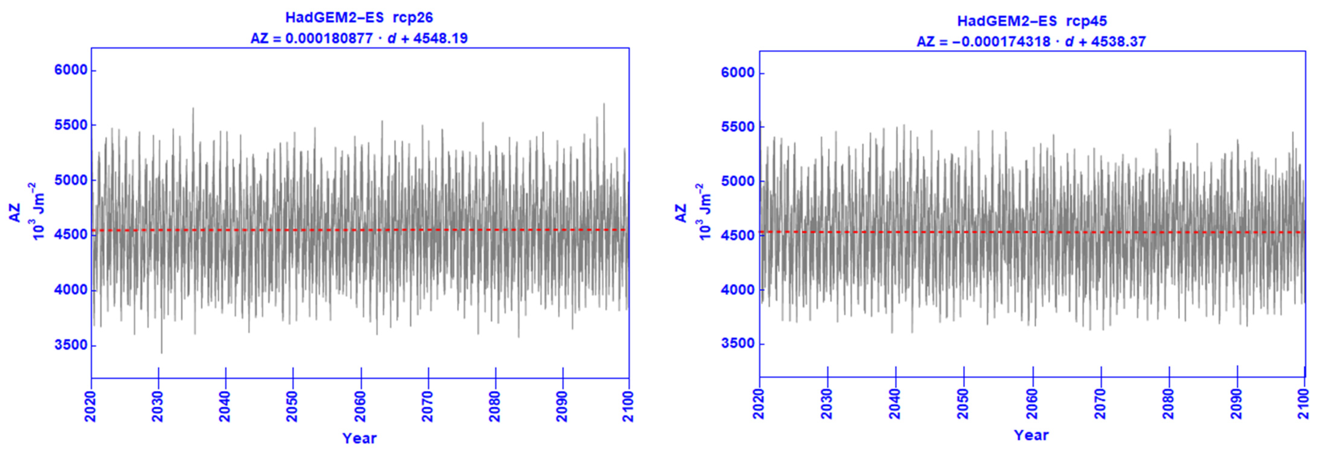
The energy balance for each of the four RCPs in the 2020–2100 period is presented in Figure 2. The values given are averages taken over the entire period. The rate of change of AZ is negative under all scenarios, but it does not seem to have any appreciable difference between rcp26 and rcp45; however, for higher concentrations, AZ decreases at a lower rate. Further, the AE rate of change is negative with almost all scenarios, decreasing faster under the extreme one. Therefore, it can be concluded that the overall effect of increased forcing is expected to be a decrease in the rate of change of the total available potential energy of the atmosphere.
The rate of change of KZ obtains a negative value under the rcp26 scenario, but under all other RCPs it is positive, with the highest values noted with the rcp60 and rcp85 forcings, indicating a tendency for strengthening of the zonal flow with time (closely related to the presence of jet-streams) with increased greenhouse gas concentrations. The respective rates for KE are negative for almost all scenarios. The decrease in the rate of change of KE noted under the extreme scenario equals the respective increase in the rate of change of KZ.
Under all RCPs, the flow of energy accomplished through the energy conversion terms is in agreement with the flow postulated by Lorenz [32] (with the only exception of the generation of eddy potential energy). It is worth reiterating here that the values in Figure 2 are long-term averages and that in the short term, the conversions may operate in different modes, as will be explained later in this section.
The conversion rates <AZ→AE> and <AZ→KZ> decrease with increasing radiative forcing, implying that the above-mentioned depletion of zonal available potential energy of the atmosphere is explained (at least partly) by its conversion into both eddy available potential energy and zonal kinetic energy but both of these conversions are less effective with increasing radiative forcing.
The conversion term <AE→KE> decreases with increasing radiative forcing too. It is interesting to note that the above-mentioned conversion <AZ→AE> that adds to the pool of AE is less than the depletion of this energy form through its conversion into KE, i.e., <AE→KE>.
The last conversion term, namely, <KE→KZ> tends to increase in response to increased forcing, explaining partly the increase in the zonal flow, discussed above; indeed, from a rate of 644.12 × 10⁻³ Wm−2 under the rcp26 scenario, KE is converted into KZ at a maximum rate of 669.37 × 10⁻³ Wm−2 under the extreme rcp85 scenario.
In general, the impact of increased radiative forcing decreases for GZ and DE but increases for GE and DZ. As explained above, the generation and dissipation terms have not been directly calculated due to their formulations in terms of frictional forces and diabatic heating rates, respectively (see [33,35,36]), which renders their direct accurate calculation with the data available on the synoptic-scale grid adopted herein not possible; hence, they are calculated as residuals in the respective Equations (1)–(4). This computational approach implicitly advocates that the generation and dissipation terms not only embrace any unresolved sub-grid scale processes, but they also accrue the computational errors from the other terms in each of the Equations (1)–(4). Nevertheless, this practice appears to be a practical alternative.
On the one hand, the direct calculation of the frictional dissipation is not feasible, bearing in mind our insufficient knowledge of friction, especially at higher elevations (see [10]). Early attempts to calculate the frictional dissipation directly in the atmosphere reveal the great knowledge gap in this respect (see [38,39]). Later attempts by using indirect methodologies [40,41] confirm the complications in obtaining a firm methodology for calculating frictional dissipation; therefore, in this study, the residual approach has been adopted in calculating DZ and DE.
On the other hand, the direct estimation of available potential energy generation from the existing mathematical formulations (see [33,35,36]) presents similar difficulties to those encountered in the direct frictional dissipation calculation. In this respect, the available potential energy generation terms are expressed as covariances of the fields of temperature and diabatic heating rates involving relationships in the form of either Equation (A2) or (A4) (see [36]). It is not possible to calculate these quantities accurately, given our insufficient knowledge of the horizontal and vertical distribution of diabatic heating rates. The residual approach is therefore adopted here too for the estimation of the generation terms, namely GZ and GE.
The generation of zonal available potential energy appears to be decreasing with increasing radiative forcing. The reverse is noted with the generation of eddy available potential energy, which increases with increasing gas concentration, from 53.5 × 10⁻³ Wm−2 under rcp26 to 126.51 × 10⁻³ Wm−2 under rcp85. The calculated changes in the dissipation of zonal kinetic energy do not seem to be largely affected under different scenarios. On the contrary, the dissipation of kinetic energy in the eddy motions tends to decrease with increasing forcing.
Further to the differences regarding the impact of different forcings on the energy cycle discussed above and which are based on the averages of the energy cycle components, some statistical measures, such as the maximum (Max), minimum (Min) and standard deviation (StDev) values have been considered. The maximum and minimum values delineate the extreme modes of operation of each of the components of the energy cycle (not necessarily occurring concomitantly); the standard deviation is a measure of the spread of these modes of operation.
The values of these statistical parameters are presented in Table 1 for the energy contents (in 103 Jm−2) and energy rates of change (in 10−3 Wm−2).
The maximum values of both the zonal available potential energy (AZ) and eddy available potential energy (AE) appear to be decreasing with increasing radiative forcing. Regarding the minimum values, for AZ there seems to be an increase with increased forcing, whereas, for AE the corresponding minimum values appear to decrease. Regarding the rates of change of the two available potential energy components, it appears that there is a tendency for decreasing rates with increasing forcing; comparing the rcp26 and the rcp85 scenarios, the decrease in amounts to 19% and the respective decrease in amounts to 18%. On the contrary, the different gas concentrations associated with each scenario do not have a noticeable impact on the changes of the minimum values of these two rates.
The maximum values of zonal kinetic energy (KZ) at which the energy cycle operates increase with increasing gas concentrations. On the contrary, the maximum value of the eddy component of kinetic energy, KE, is reached with the lowest concentration and the minimum with the extreme rcp85 scenario; with regard to the minimum values of KE, the situation is reversed, with the minimum noted with the rcp25 and the maximum with the rcp85 scenario. The extreme rcp85 scenario appears to yield the highest rates of change of both KZ and KE (i.e., and , respectively).
In Table 2, the corresponding statistical parameter values for energy conversion, generation and dissipation terms (in 10−3 Wm−2) are displayed. The maxima in the conversion between the two available potential energy forms and between the eddy components of available potential and kinetic energies, <AZ→AE> and <AE→KE>, respectively, behave rather erratically in response to the increases in greenhouse gas concentrations. The respective minima, however, exhibit a notable decrease from their values under the rcp26 scenario to their corresponding values under the rcp85 scenario.
The conversion <AZ→KZ> obtains its highest maximum values with the high concentration scenarios. It is interesting to note that the minimum values have a negative sign. From a closer examination of the values of this conversion term, as they have been calculated for each day (but also from examining the respective time series for this conversion rate, presented under Section 3.2), it was found that this term occasionally obtains negative values; this result implies that the respective underlying processes can occasionally operate in a reverse mode than what is anticipated on average, and is based on Lorenz’s postulations (this finding is also discussed in Section 3.2 below). Indeed, such as a reversal in the direction of <AZ→KZ> is quite frequent, usually lasting for several consecutive days.
The conversion rate <KE→KZ> is also found to obtain negative values, but this reversal in operation is quite rare (see also discussion in Section 3.2). The range of maximum values associated with changes in gas concentrations is quite small.
The generation term GZ is characterized by quite large maximum values, which represent the highest rates in all the terms in Equations (1)–(4). The highest maximum values for GE are quite smaller than those for its GZ counterpart. However, for both GZ and GE, the minimum values are negative, indicating that the residual approach adopted here can lead to a temporary negative generation of available potential energy. Such negative generation was quite early noted by Oort [1], even with time averaging on a hemispherical scale for GE.
The dissipation rates (DZ and DE) are positive for all RCPs at all times, in line with what is expected from the effect of frictional processes, i.e., to dissipate kinetic energy. It is noteworthy that the dissipation of kinetic energy that transforms it into thermal energy is not considered as a physical process accounted for in the Lorenz energy cycle. Nevertheless, a more recent examination of the energy cycle by Brannon [8] contemplates the feeding back of the frictionally induced thermal energy into the energy cycle.
3.2. Time Series and Trends
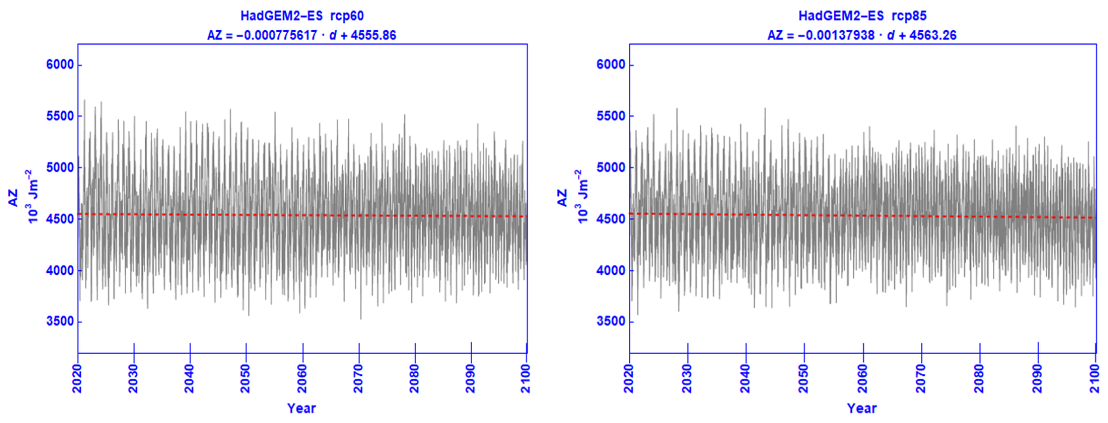
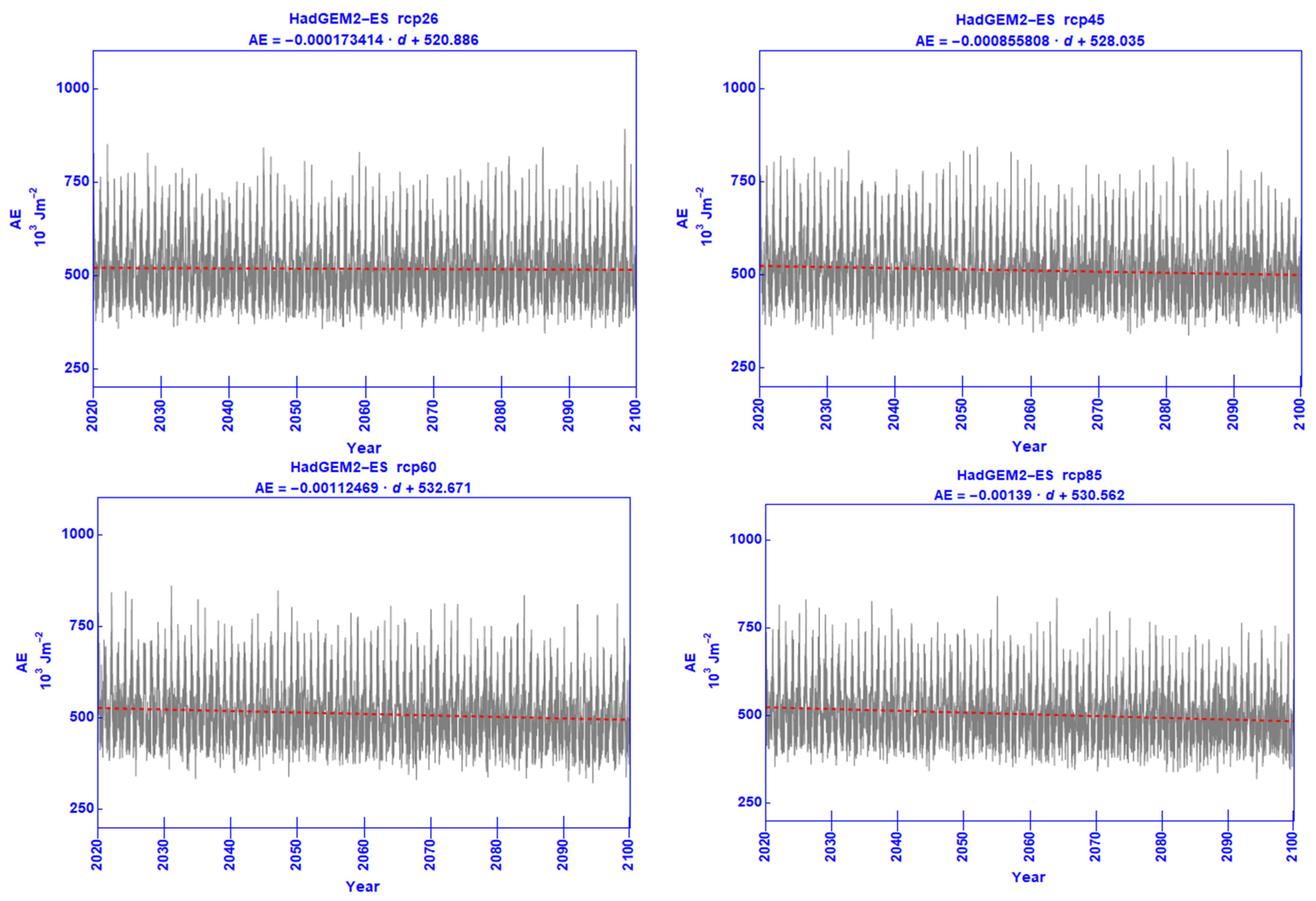
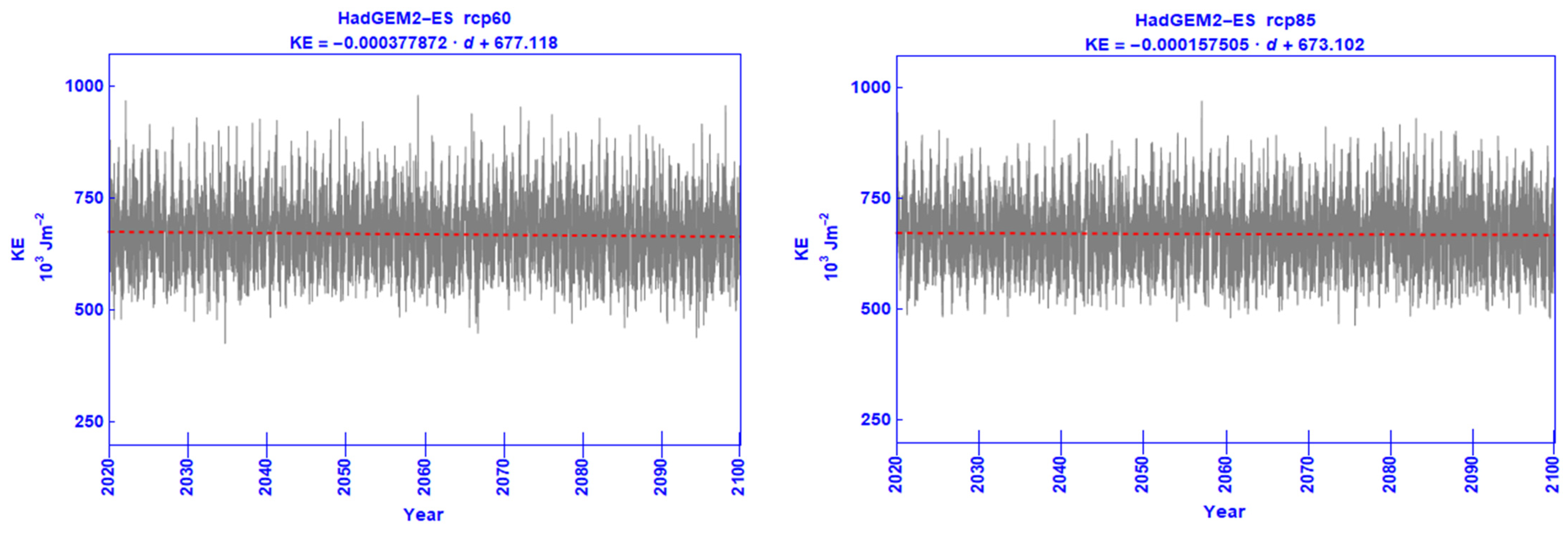
For the time period 2020–2100, the time series for the energy contents corresponding to each of the four RCP’s are shown in Figure 3, Figure 4, Figure 5 and Figure 6. These graphs show the daily values of each energy content in the period, with the linear regression equation superimposed. Similar time series graphs have been drawn for the energy conversions, available potential energy generation terms, kinetic energy dissipation terms and rates of change of energy contents but are not shown herein for the sake of brevity; however, they are all available to the reader for reference as supplementary material (see Figure S1). Further, Table 3 summarizes the numerical values of the trends for all the components of the energy cycle.
From the times series of AZ shown in Figure 3, no appreciable differences between the different scenarios are noted; other than that, the negative trend is slightly increased under the extreme one. Regarding AE, Figure 4 shows that the trend is negative under all concentrations, with a tendency to become slightly more pronounced with increasing concentrations.
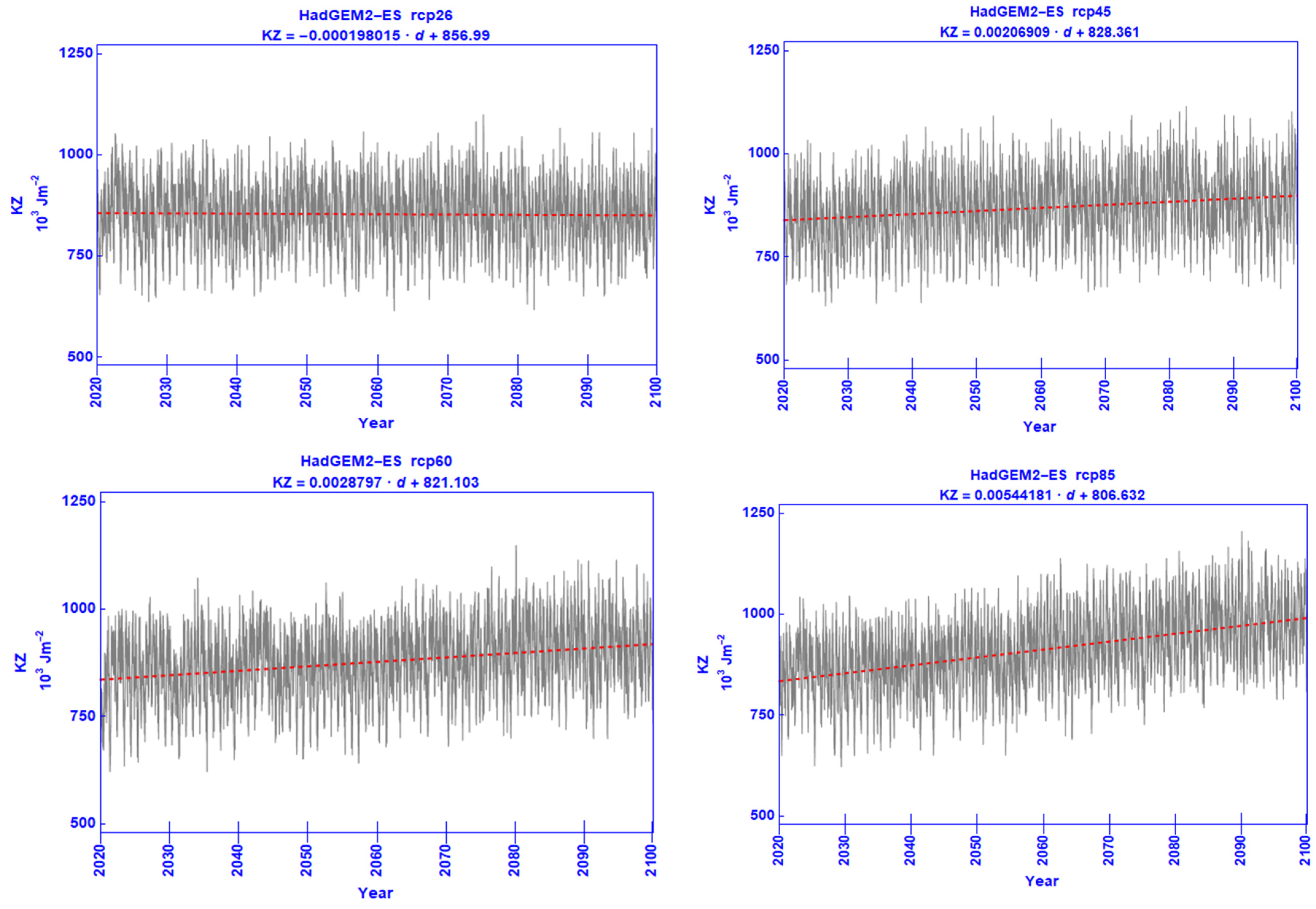
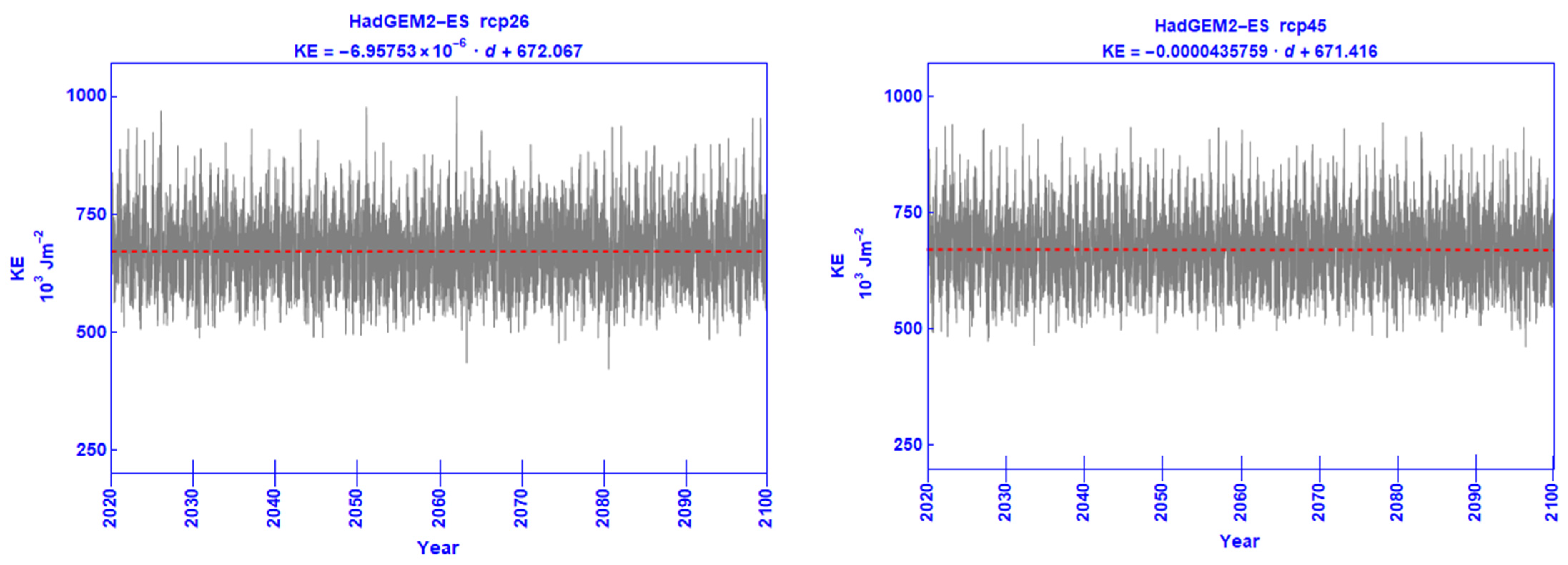
The time series for KZ is shown in Figure 5. The effect of different RCPs is easily identified: increasing forcing seems to enhance this zonal component of kinetic energy, with the rcp60 and rcp85 scenarios appearing to have the greatest effect on the increasing trend. This finding is in good agreement with the findings from the energy balance analysis in the previous section, which has led to the inference that the increase in gas concentrations could lead to an enhancement of the zonal winds as they are broadly manifested through the existence of atmospheric jet streams. The time series of the other kinetic energy component, namely KE, is shown in Figure 6. For this component, the trend appears to be negative with all the RCP scenarios, indicating a tendency for the weakening of the kinetic energy of the eddy motions.
The time series for <AZ→AE> exhibits a negative trend under all RCPs. This negative trend appears to be more pronounced under rcp85. The time series for the conversion of AZ into KZ, i.e., <AZ→KZ>, does not exhibit any appreciable change between different RCPs. Concerning the conversion term <AE→KE>, the extreme rcp85 scenario reveals a slightly decreasing trend with time. Lastly, in the time series of the conversion <KE→KZ> all scenarios but the one representing the lowest concentration (i.e., rcp26) show an increase in KZ at the expense of KE, albeit a small one.
It is interesting to note that the two conversions <AZ→AE> and <AE→KE> are always positive, irrespective of the level of radiative forcing, following the direction of energy flow of Lorenz energy cycle; with regard to the former, the horizontal and vertical transfer of sensible heat is at all times towards the lower temperature zones; with regard to the latter, there is a persistent rising of warmer air and sinking of colder air within latitude zones. However, the conversion rate <KE→KZ> appears to be negative in some rather rare cases, albeit at comparatively low rates (not below −400 × 10−3 Wm−2, see Table 2); this confirms that the prevailing eddy transport of angular momentum is towards areas of higher angular velocity thus feeding the zonal flow; nevertheless, in some cases, this process reverses its sign, thus feeding the kinetic energy of the eddies at the expense of the zonal flow. What is even more astounding is the behavior of the last conversion process, namely, <AZ→KZ> that, as explained above, is accomplished by the physical process of the sinking of colder air in colder latitude zones and rising of warmer air in warmer latitude zones. As can be seen from Figure 2, on average, this physical process indeed leads to a conversion in the direction of enhancing the zonal flow at the expense of the zonal available potential energy, as postulated by Lorenz [10,11,32,42]. However, the time series of this conversion suggests that the atmospheric engine can reverse its mode of operation, converting KZ into AZ and vice versa, and that the conversion in both directions can be of comparable magnitude (see also the minimum and maximum values of <AZ→KZ> in Table 2, −1043 × 10−3 Wm−2 and 1183 × 10−3 Wm−2, respectively).
The time series and the fitted linear regressions are in agreement with the general comments based on the mean values in Figure 2, regarding the generation of available potential energy and the dissipation of kinetic energy. Indeed, the trend for GZ decreases with increasing forcing and the reverse is noted regarding the trend for GE. Further, the trend in DZ is unaffected by the changing gas concentrations, whereas the trend in DE decreases with increasing forcing.
4. Discussion
As defined by Lorenz, the energy cycle of the atmosphere comprises a methodology that is exploited in the diagnosis of atmospheric dynamics; however, as the available potential energy concept in the Lorenz energy cycle is defined over the entire atmosphere, the application of the energetics approach to local or regional scales presents a number of limitations, as discussed by Marquet [43]. Muench [33,34] reformulated the energetics integrals to take into account the boundary transfers of energy in a limited area; in this respect, he considered the amount of available potential energy calculated over this area as the contribution of the limited area to the total available potential energy of the entire atmosphere (see also [35,36,37]).
Among the difficulties and limitations inherent in exploiting the Lorenz energy cycle concepts, one must take into consideration the necessary approximations and numerical solutions that are adopted in order to carry out the calculations with the available atmospheric data. In the present study, the data that comprise the basis for the calculations are those produced by the HadGEM2-ES model for fulfilling the needs of CMIP5. On the one hand, the results are presented in terms of the time series of the energetics components, and on the other hand, in the form of energy balances using long-term averages. The long-term averaging of the results are expected to yield a more representative picture of the energy cycle. The time variation in the energy components delineated in the time series diagrams does not comprise a means to directly interpret the results within the framework of the Lorenz energy cycle, but they have been used herein to determine possible trends.
The results of the present study show that different future climate scenarios have a different effect on the components of the energy cycle. The observed general tendency for a decrease in the available potential energy reservoirs with increasing gas concentrations (which is more pronounced for AZ rather than for AE, see Figure 2, Figure 3 and Figure 4) is ascribed to a previously noted effect of the warming of the atmosphere as a result of increased greenhouse gases. Indeed, the energetics response of the atmosphere to its warming due to increased amounts of CO2, was ascribed to the smoothing of the meridional temperature gradients (see [44,45]), which is expected to lead to a reduction of the availability of potential and internal energies for conversion into kinetic energy.
The observed increase in KZ as a result of increased radiative forcing, which is reflected in both the energy balances (Figure 2) and the trends in the respective time series (Figure 5), is ascribed primarily to an increased conversion from KE. This interpretation is dictated by the enhanced calculated conversion rate <KE→KZ>, which, together with the noted increase in KZ, yields a small increase in DZ. This finding has some important implications in the physical process that converts KE into KZ, namely, the transfer of angular momentum by the eddies towards areas of higher angular velocity, which subsequently enhances the zonal flow.
The conversion rates of available potential energy (both AZ and AE) into kinetic energy (both KZ and KE) decrease under enhanced forcing. This result is in general agreement with findings by Hernándex-Deckers and von Storch [27], who have performed calculations of the Lorenz energy cycle using simulations with the ECHAM5/MPI-OM model under different CO2 regimes. Earlier simulations with changing CO2 scenarios have also been performed by Boer [45], who had used the Canadian Climate Centre General Circulation Model to investigate the change in December–February climate for a doubling of CO2. Although his investigation was viewed from a Northern Hemisphere middle-latitude perspective, the findings are also supportive of the suppression of the intensity of atmospheric energetics with the increasing concentration of this greenhouse gas. Lucarini et al. [44] have also carried out a thermodynamically based theoretical investigation on how global warming impacts the thermodynamics of the climate system and they reached the conclusion that the climate system becomes less efficient and more irreversible, featuring higher entropy production as it becomes warmer. The above decrease in the efficiency of the atmospheric engine in converting available potential energy into kinetic energy is claimed to be due to the smoothing of the equator-to-pole temperature gradient as more greenhouse gases are accumulated into the atmosphere [27,45].
As mentioned above, Veiga and Ambrizzi [28] also studied the effect of different RCP’s on the Lorenz energy cycle by using CMIP5 model data; therefore, it is interesting to perform a brief comparative analysis of both studies, at least for the energy components that are common to both investigations.
Although the values for <AZ→KZ> estimated in the present study are less than those presented by Veiga and Ambrizzi [28] by one order of magnitude, there is a general agreement regarding the impact of increased gas concentrations on this conversion rate: in both studies, this conversion decreases with increasing greenhouse gases. The same decrease in <AZ→AE> with increasing concentrations is noted in both studies, but its corresponding values are less in the present study than in Veiga and Ambrizzi [28], albeit of the same order of magnitude. The tendency for <KE→KZ> to decrease with rising concentrations is noted in both studies, though at different rates: ranging from 644 to 669 × 10−3 Wm−2 in the present study and from 420 to 490 × 10−3 Wm−2 in the study by Veiga and Ambrizzi [28]. The conversion between the eddy components of available potential and kinetic energies, i.e., <AE→KE>, is in good agreement in both studies, both with regard to the impact of increased radiative forcing and its calculated values: indeed, herein, this rate varies from 1782 to 1801 × 10−3 Wm−2, and in Veiga and Ambrizzi [28] it varies from 2200 to 2240 × 10−3 Wm−2; also, this rate decreases slightly with increasing forcing.
Differences in the energy cycle calculated with different sets of CMIP5 are obviously expected, since differences in the climate models result in different projections (e.g., [46,47,48]) and this should be reflected in the results obtained in an energetics analysis. Further, differences in the horizontal and vertical resolution of the model projection data that are used as input in such an analysis can have an impact on the calculations. Finally, the time period represented in different energetics analyses is expected to have an impact on the results, as can be seen from the time series and trends presented in this paper (see Section 3.2).
Ideally, to objectively evaluate the Lorenz energy cycle calculated on model output data, the findings should be contrasted against an energetics analysis based on observational data referring to the same time period. Apparently, this is not feasible to accomplish in this study. Instead, an evaluation is performed, adopting an approach along similar lines to those previously discussed by Boer and Lambert [23], in which the atmospheric climate system is contemplated to operate as a heat engine.
In a conceptual atmospheric heat engine model, energy is generated (by diabatic heating processes at rates GZ and GE), converted (from one form into another at rates <AZ→AE>, <AE→KE>, <KE→KZ> and <AZ→KZ>) and finally is dissipated by frictional processes into heat (at rates DZ and DE). An appreciation of the changes in the “rate of working” of the climate system could be attained via the changes in the rates at which energy is generated (energy generation rate of working), converted (energy conversion rate of working) and dissipated (energy dissipation working rate).
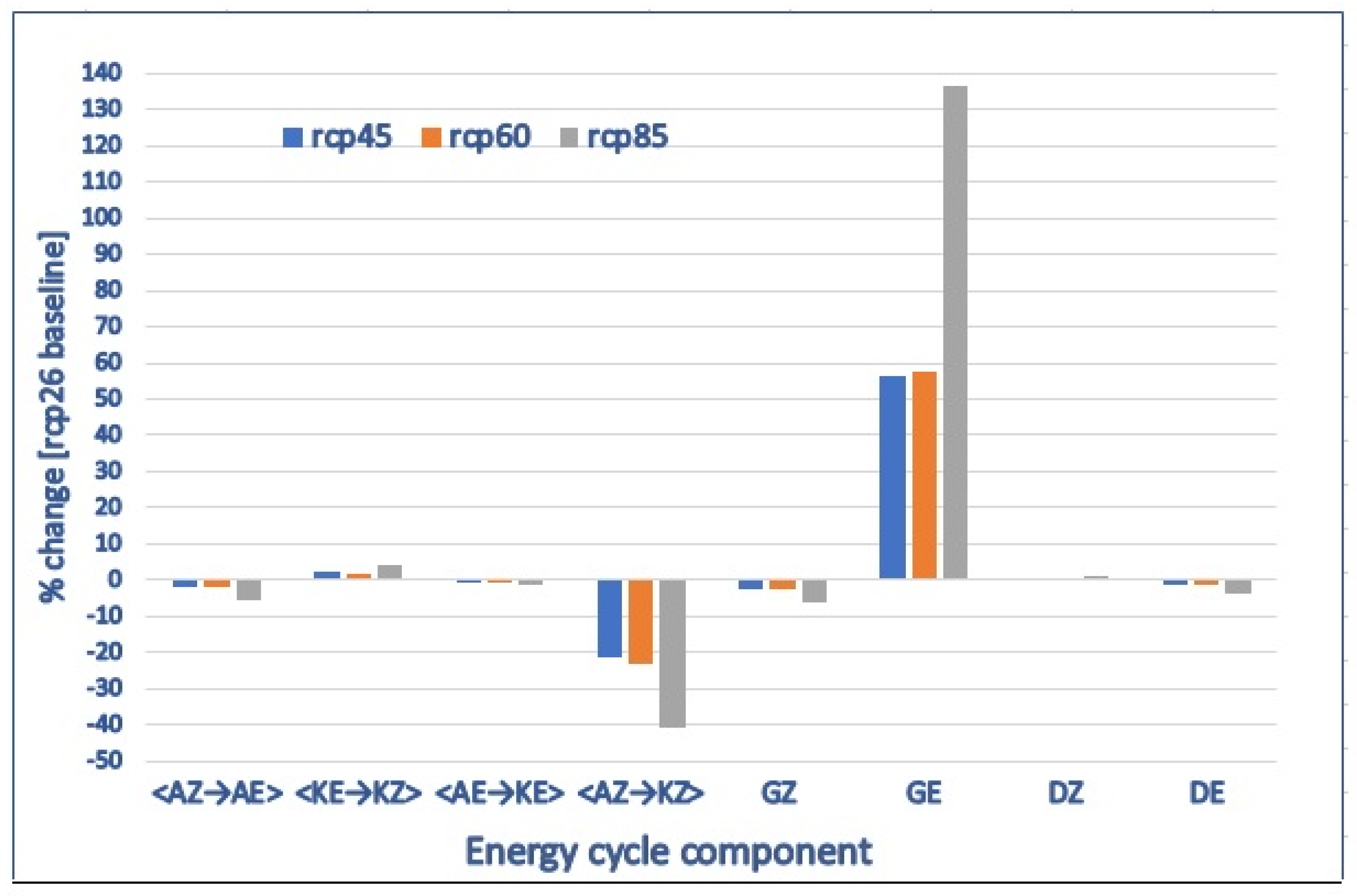
Due to the lack of results from an independent set of data that could constitute the baseline, the results of the present study are compared between them, considering the scenario with the least forcing, i.e., the rcp26, as the baseline. For the rcp45, rcp60 and rcp85 scenarios, the percentage changes in the energy conversion, generation and dissipation terms, with respect to the rcp26 baseline are displayed in Figure 7.
From this figure, it can be inferred that, with regard to the conversion rate of working, there is an overall decrease with increasing forcing, which is mostly due to an excessive rate of conversion between the zonal components of the available potential and kinetic energies. Overall, the conversion rate of working exhibits a decrease of around 5% for the rcp45 and rcp60 scenarios, but this is doubled to around 10% for the rcp85 scenario. The overall generation working rate increases by 27% for the rcp60 and rcp85, but this increase is more than doubled, reaching 65%, under the rcp85 scenario. Apparently, the increase is mostly due to the excessive increase in GE with increasing gas concentrations. Lastly, regarding the dissipation working rate, from a decrease of 0.5% under rcp45, it decreases to 0.7% under rcp60, with a further decrease reaching 1.5% under rcp85.
A related current effort by the author is underway, adopting a similar methodology for the scenarios employed in CMIP6 (Coupled Model Intercomparison Project, Phase 6) that combine different socio-economic reference assumptions with different future levels of climate forcing. The “set of SSP scenarios consists of a set of baselines, which provides a description of future developments in absence of new climate policies beyond those in place today, as well as mitigation scenarios which explore the implications of climate change mitigation policies” [49]. The combination of SSPs with RCPs yields a comprehensive application of the CMIP6 scenario matrix [50]. The major effort in this planned work is to perform an evaluation of the effect of the different CMIP6 scenarios on the Lorenz energy cycle. It should also be interesting to proceed with a comparison of the energetics of the atmosphere with projections from different models that have been used in the intercomparison project and check whether any differences are statistically significant.
Supplementary Materials
The following are available online at https://0-www-mdpi-com.brum.beds.ac.uk/article/10.3390/cli9120180/s1, Figure S1: Time series for all the energy cycle components corresponding to each Representative Concentration Pathway together with the fitted linear regression as a function of day.
Funding
This research received no external funding.
Institutional Review Board Statement
Not applicable.
Informed Consent Statement
Not applicable.
Data Availability Statement
The data that were used in this study were provided by the HadGEM2-ES Development Team, the World Climate Research Programme’s Working Group on Coupled Modelling, the Global Organization for Earth System Science Portals, the Earth System Grid Federation, the Centre for Environmental Data Analysis and the Deutsches Klimarechenzentrum GmbH.
Acknowledgments
This work was carried out within the EMME-CARE project that received funding from the European Union’s Horizon 2020 research and innovation programme under grant agreement No. 856612 and the Cyprus Government. The author wishes to thank the two anonymous reviewers for their constructive comments.
Conflicts of Interest
The author declares no conflict of interest.
Appendix A
For the numerical representation of the components of the energy cycle, a number of symbolic expressions for zonal, meridional, vertical and area averaging are introduced. In this respect, the position of a variable Xijk in the three-dimensional grid of the computational atmospheric volume is determined by the combination of three indices i, j, and k, representing its position with respect to south–north, east–west and the isobaric level numbered consecutively upwards, respectively (i = 1, 2, 3,…, 144; j = 1, 2, 3,…, 192; k = 1, 2, 3,…, 8).
In the original CMIP5 dataset generated by HadGEM2-ES model, some values of the variables in the lowest atmospheric levels are shown as NaN (Not a Number) because of the protrusion of elevated land into these levels. From an examination of the data, this land masking is not fixed but varies with time. Apparently, these NaN labels are non-numerical values that cannot propagate in the calculations and this fact was taken into consideration in the numerical computations by disregarding the grid points at which a variable is denoted as NaN.
The zonal mean of the variable that is a function of latitude and pressure level is defined by:
where δλ is the longitudinal grid distance (i.e., 1.875°) and the summation (m) in the denominator is taken over all grid points that are denoted as NaN in the raw data.
The departure from the above zonal average calculated at every grid point is defined by:
Bearing in mind the above, the numerical analog that was used herein in order to calculate the area average of a variable over the entire computational region at level k is defined as follows:
where is the latitude (in radians) at latitude zone i, δφ is the latitudinal grid distance (i.e., 1.25°) and the summation (m) in the denominator is taken over all grid points that are denoted as NaN in the raw data.
The following quantity, which is a function of latitude and pressure level, is needed in the formulation of some of the numerical analogs below and it is defined as the difference between Equations (A1) and (A3):
Within a pressure layer , the numerical analogs for the calculation of the energy quantities appearing in rates of change of Equations (1)–(4) are given by:
where the termpodynamic temperature is denoted by T and the longitudinal and latitudinal horizontal wind components are denoted by u and v, respectively. The acceleration of gravity is shown as g and
is an average value of a static stability parameter over the isobaric surface, where R is the gas constant for dry air and cp is the specific heat of air at constant pressure.
Bearing in mind that the energy quantities are defined over the entire atmosphere, the subscript k in the quantities on the left-hand side of Equations (A5)–(A8) indicates the contribution of the specified pressure layer to the total amount of the respective energy form hence integrals
Likewise, within a pressure layer , the numerical analogs for the calculation of the energy conversions are given by:
where r is the Earth’s mean radius and ω = dp/dt denotes the vertical velocity in the coordinate system used here, in which p is the vertical coordinate. As above, the subscript k on the left-hand side of Equations (A10)–(A13) indicates the contribution of the respective atmospheric layer to the total integral.
In Equations (A10)–(A13), the following symbolic representation of a finite-difference in the vertical sense has been adopted:
Similarly, the finite-difference symbol in the meridional sense is given by:
Finally, for the vertical integration of the right-hand side terms in Equations (A5)–(A8) and (A9)–(A13) and over the entire atmospheric volume considered in this study (i.e., from 1000 to 10 hPa), a trapezoidal rule is adopted.
References
- Oort, A.H. On estimates of the atmospheric energy cycle. Mon. Weather Rev. 1964, 92, 483–493. [Google Scholar] [CrossRef] [Green Version]
- Saltzman, B. Large-scale atmospheric energetics in the wave-number domain. Rev. Geophys. 1970, 8, 289–302. [Google Scholar] [CrossRef]
- Wiin-Nielsen, A. On the intensity of the general circulation of the atmosphere. Rev. Geophys. 1968, 6, 559–579. [Google Scholar] [CrossRef]
- Margules, M. Über die Energie der Stürme (On the energy of storms—Originally published by the Imperial Central Institute for Meteorology, Vienna, Austria, 1903; pp. 1–26). In The Mechanics of the Earth’s Atmosphere—A Collection of Translations; Abbe, C., Ed.; English translation by Smithsonian Institution: Washington, DC, USA, 1904; Volume 51, pp. 533–595. [Google Scholar]
- Lorenz, E.N. Energy and numerical weather prediction. Tellus 1960, 12, 364–373. [Google Scholar] [CrossRef] [Green Version]
- Van Mieghem, J. Atmospheric Energetics; Clarendon Press: Oxford, UK, 1973. [Google Scholar]
- Pearce, R.P. On the concept of available potential energy. Q. J. R. Meteorol. Soc. 1978, 104, 737–755. [Google Scholar] [CrossRef]
- Bannon, P.R. Atmospheric available energy. J. Atmos. Sci. 2012, 69, 3733–3744. [Google Scholar] [CrossRef]
- Aranha, A.F.; Veiga, J.A.P. An analysis of the spectral energetics for a planet experiencing rapid greenhouse gas emissions. Atmos. Clim. Sci. 2017, 7, 117–126. [Google Scholar] [CrossRef] [Green Version]
- Lorenz, E.N. The Nature and Theory of the General Circulation of the Atmosphere; World Meteorological Organization: Geneva, Switzerland, 1967. [Google Scholar]
- Lorenz, E.N. Available potential energy and the maintenance of the general circulation. Tellus 1955, 7, 157–167. [Google Scholar] [CrossRef] [Green Version]
- Krueger, A.F.; Winston, J.S.; Haines, D.A. Computations of atmospheric energy and its transformation for the Northern Hemisphere for a recent five-year period. Mon. Weather Rev. 1965, 93, 227–238. [Google Scholar] [CrossRef]
- Dutton, J.A.; Johnson, D.R. The theory of available potential energy and a variational approach to atmospheric energetics. Adv. Geophys. 1967, 12, 333–436. [Google Scholar]
- Wiin-Nielsen, A. On the annual variation and spectral distribution of atmospheric energy. Tellus 1967, 19, 540–559. [Google Scholar] [CrossRef]
- Oort, A.H.; Peixóto, J.P. The annual cycle of the energetics of the atmosphere on a planetary scale. J. Geophys. Res. 1974, 79, 2705–2719. [Google Scholar] [CrossRef]
- Oriol, E. Energy Budget Calculations at ECMWF—Part 1: Analyses 1980–81. Technical Report, 35; ECMWF: Reading, UK, 1982. [Google Scholar]
- Kung, E.C.; Tanaka, H. Energetics analysis of the global circulation during the special observation periods of FGGE. J. Atmos. Sci. 1983, 40, 2575–2592. [Google Scholar] [CrossRef] [Green Version]
- Ulbrich, U.; Speth, P. The global energy cycle of stationary and transient atmospheric waves: Results from ECMWF analyses. Meteorol. Atmos. Phys. 1991, 45, 125–138. [Google Scholar] [CrossRef]
- Hu, Q.; Tawaye, Y.; Feng, S. Variations of the northern hemisphere atmospheric energetics: 1948–2000. J. Clim. 2004, 17, 1975–1986. [Google Scholar] [CrossRef]
- Marques, C.A.F.; Castanheira, J.M. A detailed normal-mode energetics of the general circulation of the atmosphere. J. Atmos. Sci. 2012, 69, 2718–2732. [Google Scholar] [CrossRef]
- Kalnay, E.; Kanamitsu, M.; Kistler, R.; Collins, W.; Deaven, D.; Gandin, L.; Iredell, M.; Saha, S.; White, G.; Woollen, J.; et al. The NCEP/NCAR 40-year reanalysis project. Bull. Am. Meteorol. Soc. 1996, 77, 437–471. [Google Scholar] [CrossRef] [Green Version]
- Uppala, S.M.; Kållberg, P.W.; Simmons, A.J.; Andrae, U.; da Costa Bechtold, V.; Fiorino, M.; Gibson, J.K.; Haseler, J.; Hernandez, A.; Kelly, G.A.; et al. The ERA-40 re-analysis. Q. J. R. Meteorol. Soc. 2005, 131, 2961–3012. [Google Scholar] [CrossRef]
- Boer, G.J.; Lambert, S. The energy cycle in atmospheric models. Clim. Dyn. 2008, 30, 371–390. [Google Scholar] [CrossRef]
- Taylor, K.E.; Stouffer, R.J.; Meehl, G.A. An overview of CMIP5 and the experiment design. Bull. Am. Meteorol. Soc. 2012, 93, 485–498. [Google Scholar] [CrossRef] [Green Version]
- Moss, R.H.; Edmonds, J.A.; Hibbard, K.A.; Manning, M.R.; Rose, S.K.; Van Vuuren, D.P.; Carter, T.R.; Emori, S.; Kainuma, M.; Kram, T.; et al. The next generation of scenarios for climate change research and assessment. Nature 2010, 463, 747–756. [Google Scholar] [CrossRef]
- Gleckler, P. The AMIP Experience: Challenges and Opportunities. Available online: https://digital.library.unt.edu/ark:/67531/metadc1406844/m1/1/ (accessed on 7 November 2021).
- Hernández-Deckers, D.; von Storch, J.S. Energetics responses to increases in greenhouse gas concentration. J. Clim. 2010, 23, 3874–3887. [Google Scholar] [CrossRef] [Green Version]
- Veiga, J.A.P.; Ambrizzi, T. A global and hemispherical analysis of the Lorenz energetics based on the representative concentration pathways used in CMIP5. Adv. Meteorol. 2013, 2013, 485047. [Google Scholar] [CrossRef] [Green Version]
- Jones, C.D.; Hughes, J.K.; Bellouin, N.; Hardiman, S.C.; Jones, G.S.; Knight, J.; Liddicoat, S.; O’Connor, F.M.; Andres, R.J.; Bell, C.; et al. The HadGEM2-ES implementation of CMIP5 centennial simulations. Geosci. Model Dev. 2011, 4, 543–570. [Google Scholar] [CrossRef] [Green Version]
- Collins, W.J.; Bellouin, N.; Doutriaux-Boucher, M.; Gedney, N.; Halloran, P.; Hinton, T.; Hughes, J.; Jones, C.D.; Joshi, M.; Liddicoat, S.; et al. Development and evaluation of an Earth-System model—HadGEM2. Geosci. Model Dev. 2011, 4, 1051–1075. [Google Scholar] [CrossRef] [Green Version]
- Martin, G.M.; Bellouin, N.; Collins, W.J.; Culverwell, I.D.; Halloran, P.R.; Hardiman, S.C.; Hinton, T.J.; Jones, C.D.; McDonald, R.E.; McLaren, A.J.; et al. The HadGEM2 family of Met Office Unified Model climate configurations. Geosci. Model Dev. 2011, 4, 723–757. [Google Scholar]
- Lorenz, E.N. Energetics of atmospheric circulation. Int. Dict. Geophys. 1965, 66, 1–9. [Google Scholar]
- Muench, H.S. On the dynamics of the wintertime stratosphere circulation. J. Atmos. Sci. 1965, 22, 349–360. [Google Scholar] [CrossRef] [Green Version]
- Muench, H.S. Stratospheric Energy Processes and Associated Atmospheric Long-Wave Structure in Winter; Office of Aerospace Research, United States Air Force: Cambridge, MA, USA, 1965. [Google Scholar]
- Reiter, E. Atmospheric Transport Processes—Part 1: Energy Transfers and Transformations; Available as TID-24868 from the Clearinghouse for Federal Scientific and Technical Information U. S. Department of Commerce; U.S. Atomic Energy Commission: Springfield, VA, USA, 1969; ISBN 9788578110796.
- Michaelides, S.C. Limited area energetics of Genoa cyclogenesis. Mon. Weather Rev. 1987, 115, 13–26. [Google Scholar] [CrossRef]
- Michaelides, S.C. A spatial and temporal energetics analysis of a baroclinic disturbance in the Mediterranean. Mon. Weather Rev. 1992, 120, 1224–1243. [Google Scholar] [CrossRef]
- Sverdrup, H.U. Der nordatlantische Passat; Geophysikalischen Instituts der Karl-Marx-Universität: Leipzig, Germany, 1917; Volume 2. [Google Scholar]
- Brunt, D. XLIII. Energy in the Earth’s atmosphere. Lond. Edinb. Dublin Philos. Mag. J. Sci. 1926, 1, 523–532. [Google Scholar] [CrossRef]
- Holopainen, E.O. On the dissipation of kinetic energy in the atmosphere. Tellus 1963, 15, 26–32. [Google Scholar] [CrossRef]
- Kung, E.C. Large-scale balance of kinetic energy in the atmosphere. Mon. Weather Rev. 1966, 94, 627–640. [Google Scholar] [CrossRef] [Green Version]
- Lorenz, E.N. Generation of available potential energy and the intensity of the general circulation. In Dynamics of Climate; Pfeffer, R.L., Ed.; Pergamon Press: Oxford, UK, 1960; pp. 86–92. [Google Scholar]
- Marquet, P. On the concept of exergy and available enthalpy: Application to atmospheric energetics. Q. J. R. Meteorol. Soc. 1991, 117, 449–475. [Google Scholar] [CrossRef]
- Lucarini, V.; Fraedrich, K.; Lunkeit, F. Thermodynamics of climate change: Generalized sensitivities. Atmos. Chem. Phys. 2010, 10, 9729–9737. [Google Scholar] [CrossRef] [Green Version]
- Boer, G.J. Some dynamical consequences of greenhouse gas warming. Atmos. Ocean 1995, 33, 731–751. [Google Scholar] [CrossRef]
- Miao, C.; Duan, Q.; Sun, Q.; Huang, Y.; Kong, D.; Yang, T.; Ye, A.; Di, Z.; Gong, W. Assessment of CMIP5 climate models and projected temperature changes over Northern Eurasia. Environ. Res. Lett. 2014, 9, 055007. [Google Scholar] [CrossRef]
- Díaz-Esteban, Y.; Raga, G.B.; Rodríguez, O.O.D. A weather-pattern-based evaluation of the performance of CMIP5 models over Mexico. Climate 2020, 8, 5. [Google Scholar] [CrossRef] [Green Version]
- Kravtsov, S. Pronounced differences between observed and CMIP5-simulated multidecadal climate variability in the twentieth century. Geophys. Res. Lett. 2017, 44, 5749–5757. [Google Scholar] [CrossRef]
- Riahi, K.; van Vuuren, D.P.; Kriegler, E.; Edmonds, J.; O’Neill, B.C.; Fujimori, S.; Bauer, N.; Calvin, K.; Dellink, R.; Fricko, O.; et al. The Shared Socioeconomic Pathways and their energy, land use, and greenhouse gas emissions implications: An overview. Glob. Environ. Chang. 2017, 42, 153–168. [Google Scholar] [CrossRef] [Green Version]
- van Vuuren, D.P.; Kriegler, E.; O’Neill, B.C.; Ebi, K.L.; Riahi, K.; Carter, T.R.; Edmonds, J.; Hallegatte, S.; Kram, T.; Mathur, R.; et al. A new scenario framework for Climate Change Research: Scenario matrix architecture. Clim. Chang. 2014, 122, 373–386. [Google Scholar] [CrossRef] [Green Version]
Figure 1.
Lorenz energy cycle in the atmosphere. Zonal and eddy available potential energies are denoted by AZ and AE, respectively, while zonal and eddy kinetic energies are denoted by KZ and KE, respectively; rates of change of these energy forms are shown in the boxes as local derivatives with respect to time (t). For any two forms of energy, e.g., X and Y, the conversion of the former into the latter is shown as <X→Y>. The diabatic generation of AZ and AE is denoted by GZ and GE, respectively, and the dissipation of KZ and KE is denoted by DZ and DE, respectively.

Figure 2.
Mean Lorenz energy cycle for the four RCPs shown on the top left of each diagram. Units are in 10−3 Wm−2.
Figure 2.
Mean Lorenz energy cycle for the four RCPs shown on the top left of each diagram. Units are in 10−3 Wm−2.


Figure 3.
Time series for AZ corresponding to each Representative Concentration Pathway: rcp26 (top left), rcp45 (top right), rcp60 (bottom left, and rcp85 (bottom right). The fitted linear regression for this energy content is given at the top of each diagram as a function of day (d).
Figure 3.
Time series for AZ corresponding to each Representative Concentration Pathway: rcp26 (top left), rcp45 (top right), rcp60 (bottom left, and rcp85 (bottom right). The fitted linear regression for this energy content is given at the top of each diagram as a function of day (d).


Figure 4.
Same as Figure 3 but for AE.
Figure 4.
Same as Figure 3 but for AE.

Figure 5.
Same as Figure 3 but for KZ.
Figure 5.
Same as Figure 3 but for KZ.

Figure 6.
Same as Figure 3 but for KΕ.
Figure 6.
Same as Figure 3 but for KΕ.


Figure 7.
Percent change of Lorenz energy cycle components, considering the rcp26 as a baseline.


Table 1.
Energy forms and their rates of change. Units: energies in 103 Jm−2, rates of change in 10−3 Wm−2.
Table 1.
Energy forms and their rates of change. Units: energies in 103 Jm−2, rates of change in 10−3 Wm−2.
| RCP | Statistic | AZ | AE | KZ | KE | ∂AZ/∂t | ∂AE/∂t | ∂KZ/∂t | ∂KE/∂t |
|---|---|---|---|---|---|---|---|---|---|
| rcp26 | Max | 5702.00 | 892.00 | 1099.00 | 1001.00 | 5983.80 | 1076.39 | 694.44 | 1296.30 |
| Min | 3430.00 | 345.00 | 614.00 | 422.00 | −4317.13 | −1134.26 | −740.74 | −1273.15 | |
| StDev | 345.54 | 78.95 | 74.12 | 67.88 | 747.05 | 234.60 | 151.07 | 271.63 | |
| rcp45 | Max | 5560.00 | 843.00 | 1115.00 | 944.00 | 4317.13 | 1134.26 | 659.72 | 1168.98 |
| Min | 3603.00 | 328.00 | 631.00 | 462.00 | −3738.43 | −1250.00 | −648.15 | −1250.00 | |
| StDev | 334.20 | 78.24 | 77.16 | 68.52 | 746.70 | 231.63 | 149.75 | 271.66 | |
| rcp60 | Max | 5665.00 | 861.00 | 1148.00 | 980.00 | 4722.22 | 949.07 | 729.17 | 1076.39 |
| Min | 3528.00 | 322.00 | 621.00 | 426.00 | −3761.57 | −1111.11 | −717.59 | −1238.43 | |
| StDev | 346.83 | 79.24 | 79.35 | 69.81 | 754.14 | 235.13 | 152.78 | 277.14 | |
| rcp85 | Max | 5584.00 | 840.00 | 1205.00 | 970.00 | 4861.11 | 879.63 | 833.33 | 1354.17 |
| Min | 3571.00 | 319.00 | 622.00 | 464.00 | −3969.91 | −1145.83 | −694.44 | −1134.26 | |
| StDev | 323.40 | 75.93 | 89.24 | 68.17 | 737.18 | 227.13 | 155.40 | 275.54 |
Table 2.
Energy conversion, generation and dissipation terms. Units are in 10−3 Wm−2.
| RCP | Statistic | <AZ→AE> | <AE→KE> | <KE→KZ> | <AZ→KZ> | GZ | GE | DZ | DE |
|---|---|---|---|---|---|---|---|---|---|
| rcp26 | Max | 3781.00 | 3605.00 | 2226.00 | 1183.00 | 7062.30 | 908.13 | 1448.91 | 1940.83 |
| Min | 456.00 | 633.00 | −400.00 | −1043.00 | −2183.24 | −806.80 | 144.91 | 544.94 | |
| StDev | 412.11 | 338.09 | 284.60 | 277.55 | 615.99 | 217.52 | 156.14 | 180.83 | |
| rcp45 | Max | 3707.00 | 3493.00 | 2102.00 | 1130.00 | 5819.13 | 1025.31 | 1499.94 | 2043.61 |
| Min | 231.00 | 646.00 | −612.00 | −1229.00 | −1235.26 | −829.76 | 115.82 | 465.44 | |
| StDev | 410.42 | 342.51 | 290.34 | 280.47 | 620.38 | 221.72 | 158.90 | 178.64 | |
| rcp60 | Max | 3838.00 | 3356.00 | 2050.00 | 1350.00 | 6000.91 | 943.24 | 1459.37 | 1955.83 |
| Min | 268.00 | 602.00 | −791.00 | −1081.00 | −1730.57 | −879.61 | 176.59 | 451.69 | |
| StDev | 416.45 | 344.25 | 291.76 | 281.11 | 627.65 | 222.37 | 159.345 | 181.46 | |
| rcp85 | Max | 3570.00 | 3568.00 | 2102.00 | 1255.00 | 6139.11 | 1072.39 | 1488.61 | 2001.39 |
| Min | 252.00 | 521.00 | −331.00 | −1168. | −1906.41 | −751.89 | 93.70 | 441.89 | |
| StDev | 409.87 | 345.54 | 295.75 | 291.448 | 621.44 | 228.30 | 166.437 | 182.39 |
Table 3.
The numerical values of the constants in the regression equation X = a d + b, where X denotes an energy component and d is number of the day in the 2020–2110 period.
Table 3.
The numerical values of the constants in the regression equation X = a d + b, where X denotes an energy component and d is number of the day in the 2020–2110 period.
| Energy Component | rcp26 | rcp45 | rcp60 | rcp85 | ||||
|---|---|---|---|---|---|---|---|---|
| a | b | a | b | a | b | a | b | |
| AZ | 0.000180877 | 4548.19 | −0.000174318 | 4538.37 | −0.000775617 | 4555.86 | −0.00137938 | 4563.26 |
| AE | −0.000173414 | 520.886 | −0.000855808 | 528.035 | −0.00112469 | 532.671 | −0.0139 | 530.562 |
| KZ | −0.000198015 | 856.99 | 0.00206909 | 828.361 | 0.0028797 | 821.103 | 0.00544181 | 806.632 |
| KE | −0.000006957 | 672.067 | −0.0000435769 | 671.416 | −0.000377872 | 677.118 | −0.000157505 | 673.102 |
| <AZ→AE> | −0.000727695 | 1761.81 | −0.00406241 | 1793.51 | −0.00526606 | 1813.36 | −0.0091761 | 1834.56 |
| <AE→KE> | 0.0000681611 | 1799.87 | −0.000578684 | 1809.23 | −0.000711477 | 1809.16 | −0.00188323 | 1819.13 |
| <KE→KZ> | −0.0000463435 | 645.031 | 0.0010757 | 636.46 | 0.00151958 | 626.78 | 0.00222846 | 625.985 |
| <AZ→KZ> | 0.00012192 | 44.8891 | −0.000619308 | 49.3058 | −0.00095322 | 54.9834 | −0.00134682 | 54.287 |
| GZ | −0.000603186 | 1806.53 | −0.00464604 | 1841.96 | −0.00619399 | 1867.8 | −0.0104915 | 1888.16 |
| GE | 0.000814931 | 37.6362 | 0.00350392 | 15.3122 | 0.00457072 | −4.51968 | 0.00730985 | −15.8114 |
| DZ | 0.0000805303 | 689.841 | 0.000446787 | 685.912 | 0.000579014 | 681.446 | 0.000885082 | 680.156 |
| DE | 0.000103154 | 1155.08 | −0.00166409 | 1173.02 | −0.00224273 | 1182.61 | −0.00413184 | 1193.6 |
| ∂AZ/∂t | 0.00000617363 | −0.234767 | 0.0000359286 | −0.861479 | 0.0000229027 | −0.506591 | 0.0000364437 | −0.771435 |
| ∂AE/∂t | 0.0000213124 | −0.453647 | 0.0000184446 | −0.360312 | 0.0000132693 | −0.276031 | 0.0000111378 | −0.296424 |
| ∂KZ/∂t | −0.00000413516 | 0.0599288 | 0.0000111867 | −0.194471 | −0.000013008 | 0.317168 | 0.000000572 | 0.0563835 |
| ∂KE/∂t | 0.00000907443 | −0.192631 | 0.0000100373 | −0.252894 | 0.0000121827 | −0.231162 | 0.0000181658 | −0.414366 |
Publisher’s Note: MDPI stays neutral with regard to jurisdictional claims in published maps and institutional affiliations. |
© 2021 by the author. Licensee MDPI, Basel, Switzerland. This article is an open access article distributed under the terms and conditions of the Creative Commons Attribution (CC BY) license (https://creativecommons.org/licenses/by/4.0/).
Share and Cite
MDPI and ACS Style
Michaelides, S. Lorenz Atmospheric Energy Cycle in Climatic Projections. Climate 2021, 9, 180. https://0-doi-org.brum.beds.ac.uk/10.3390/cli9120180
AMA Style
Michaelides S. Lorenz Atmospheric Energy Cycle in Climatic Projections. Climate. 2021; 9(12):180. https://0-doi-org.brum.beds.ac.uk/10.3390/cli9120180
Chicago/Turabian StyleMichaelides, Silas. 2021. "Lorenz Atmospheric Energy Cycle in Climatic Projections" Climate 9, no. 12: 180. https://0-doi-org.brum.beds.ac.uk/10.3390/cli9120180
Note that from the first issue of 2016, this journal uses article numbers instead of page numbers. See further details here.