
Long-Term Changes of Aquatic Invasive Plants and Implications for Future Distribution: A Case Study Using a Tank Cascade System in Sri Lanka

 , , and
Abstract
:1. Introduction
2. Materials and Methods
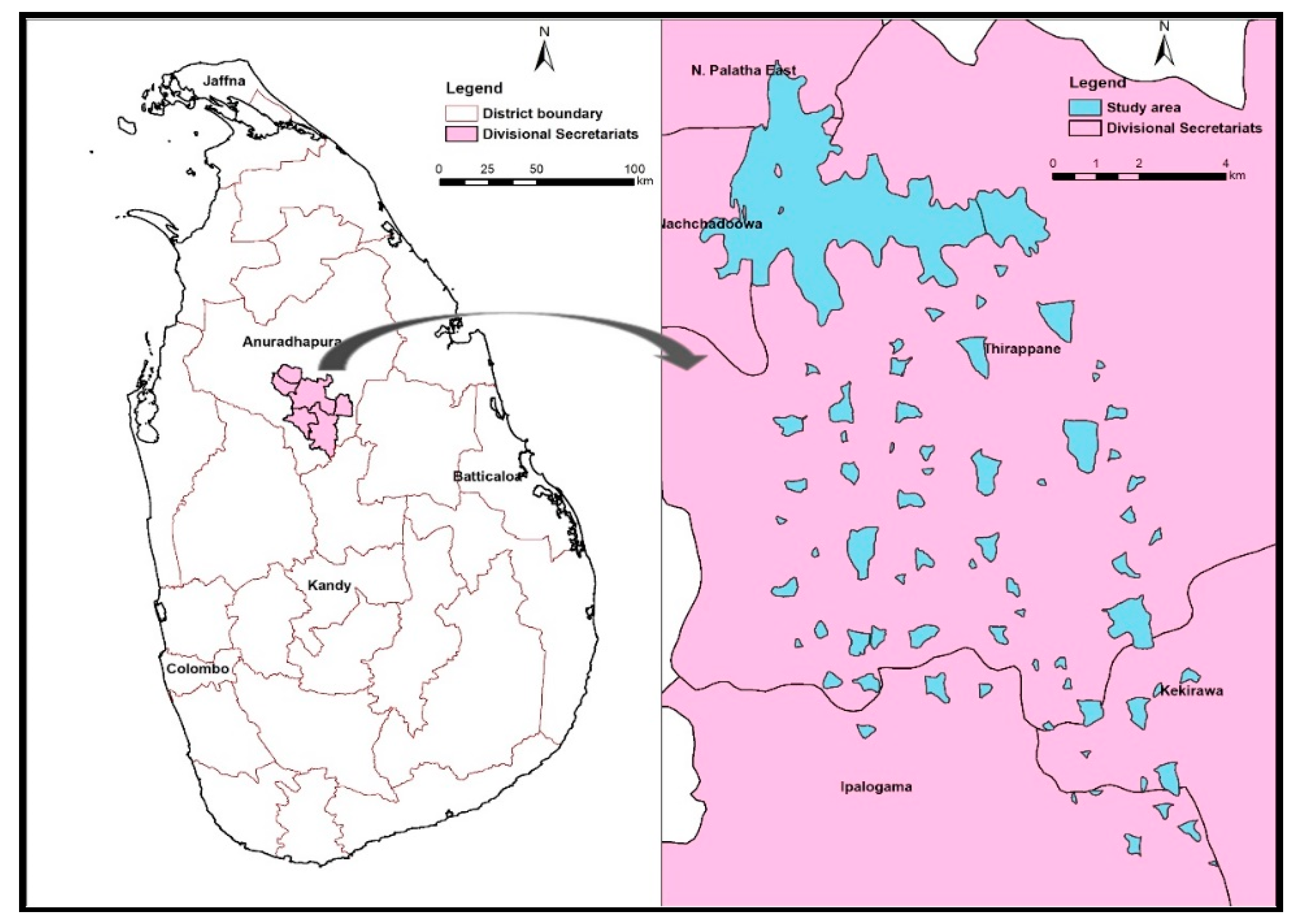
2.1. Study Area
2.2. Analysis of Satellite Images to Assess AIAPs Distribution
2.2.1. Landsat Data
2.2.2. Image Processing
2.2.3. Accuracy Assessment
2.3. Long-Term Trend Analysis of Climate Variables
3. Results
3.1. Accuracy Assessment and Land Use
3.2. Long-Term Trend Analysis of Climate Variables
4. Discussion
5. Limitations and Challenges of the Study
6. Conclusions
Author Contributions
Funding
Data Availability Statement
Acknowledgments
Conflicts of Interest
References
- Havel, J.E.; Kovalenko, K.E.; Thomaz, S.M.; Amalfitano, S.; Kats, L.B. Aquatic invasive species: Challenges for the future. Hydrobiologia 2015, 750, 147–170. [Google Scholar] [CrossRef]
- Dudgeon, D.; Arthington, A.H.; Gessner, M.O.; Kawabata, Z.-I.; Knowler, D.J.; Lévêque, C.; Naiman, R.J.; Prieur-Richard, A.-H.; Soto, D.; Stiassny, M.L. Freshwater biodiversity: Importance, threats, status and conservation challenges. Biol. Rev. 2006, 81, 163–182. [Google Scholar] [CrossRef]
- Millennium Ecosystem Assessment. Ecosystems and Human Well-Being: Synthesis; Island Press: Washington, DC, USA, 2005. [Google Scholar]
- Abell, R. Conservation biology for the biodiversity crisis: A freshwater follow-up. Conserv. Biol. 2002, 16, 1435–1437. [Google Scholar] [CrossRef] [Green Version]
- Secretariat of the Convention on Biological Diversity. Global Biodiversity Outlook 4; Secretariat of the Convention on Biological Diversity: Montréal, QC, Canada, 2014; p. 155. [Google Scholar]
- Stiers, I.; Crohain, N.; Josens, G.; Triest, L. Impact of three aquatic invasive species on native plants and macroinvertebrates in temperate ponds. Biol. Invasions 2011, 13, 2715–2726. [Google Scholar] [CrossRef]
- Gallardo, B.; Clavero, M.; Sánchez, M.I.; Vilà, M. Global ecological impacts of invasive species in aquatic ecosystems. Glob. Chang. Biol. 2016, 22, 151–163. [Google Scholar] [CrossRef]
- Boylen, C.W.; Eichler, L.W.; Madsen, J.D. Loss of native aquatic plant species in a community dominated by Eurasian watermilfoil. Hydrobiologia 1999, 415, 207–211. [Google Scholar] [CrossRef]
- McCormick, F.H.; Contreras, G.C.; Johnson, S.L. Effects of nonindigenous invasive species on water quality and quantity. A Dyn. Invasive Species Res. Vis. Oppor. Priorities 2009, 29, 111–120. [Google Scholar]
- Mironga, J.M.; Mathooko, J.; Onywere, S. The effect of water hyacinth (Eichhornia crassipes) infestation on phytoplankton productivity in Lake Naivasha and the status of control. J. Environ. Sci. Eng. 2011, 5, 1252–1260. [Google Scholar]
- Room, P.; Fernando, I. Weed invasions countered by biological control: Salvinia molesta and Eichhornia crassipes in Sri Lanka. Aquat. Bot. 1992, 42, 99–107. [Google Scholar] [CrossRef]
- Villamagna, A.; Murphy, B. Ecological and socio-economic impacts of invasive water hyacinth (Eichhornia crassipes): A review. Freshw. Biol. 2010, 55, 282–298. [Google Scholar] [CrossRef]
- Giller, P.S.; Hillebrand, H.; Berninger, U.G.; Gessner, O.M.; Hawkins, S.; Inchausti, P.; Inglis, C.; Leslie, H.; Malmqvist, B.; T. Monaghan, T.M. Biodiversity effects on ecosystem functioning: Emerging issues and their experimental test in aquatic environments. Oikos 2004, 104, 423–436. [Google Scholar] [CrossRef]
- Tilman, D.; Lehman, C. Human-caused environmental change: Impacts on plant diversity and evolution. Proc. Natl. Acad. Sci. USA 2001, 98, 5433–5440. [Google Scholar] [CrossRef] [Green Version]
- Holm, L.G.; Weldon, L.W.; Blackburn, R.D. Aquatic Weeds. Sci. New Ser. 1969, 166, 699–709. [Google Scholar] [CrossRef]
- Weiss, J.; Dugdale, T. Part 2-Impacts of priority wetland weeds. In Knowledge Document of the Impact of Priority Wetland Weeds; Department of Environment, Land, Water and Planning (DELWP): Victoria, Australia, 2017; p. 81. [Google Scholar]
- Holm, L.; Weldon, L.; Blackburn, R. Aquatic weeds. Science 1969, 166, 699–709. [Google Scholar] [CrossRef]
- Cubasch, U.; Wuebbles, D.; Chen, D.; Facchini, M.C.; Frame, D.; Mahowald, N.; Winther, J.-G. Introduction. In Climate Change 2013: The Physical Science Basis. Contribution of Working Group I to the Fifth Assessment Report of the Intergovernmental Panel on Climate Change; Stocker, T.F., Qin, D., Plattner, G.-K.M., Tignor, S.K.A., Boschung, J., Nauels, A.Y., Xia, V.B., Midgley, P.M., Eds.; Cambridge University Press: Cambridge, UK; New York, NY, USA, 2013. [Google Scholar]
- Rahel, F.J.; Olden, J.D. Assessing the effects of climate change on aquatic invasive species. Conserv. Biol. 2008, 22, 521–533. [Google Scholar] [CrossRef] [PubMed]
- Bellard, C.; Jeschke, J.M.; Leroy, B.; Mace, G.M. Insights from modeling studies on how climate change affects invasive alien species geography. Ecol. Evol. 2018, 8, 5688–5700. [Google Scholar] [CrossRef] [PubMed]
- Pratchett, M.S.; Bay, L.K.; Gehrke, P.C.; Koehn, J.D.; Osborne, K.; Pressey, R.L.; Sweatman, H.P.; Wachenfeld, D. Contribution of climate change to degradation and loss of critical fish habitats in Australian marine and freshwater environments. Mar. Freshw. Res. 2011, 62, 1062–1081. [Google Scholar] [CrossRef] [Green Version]
- Burgmer, T.; Hillebrand, H.; Pfenninger, M. Effects of climate-driven temperature changes on the diversity of freshwater macroinvertebrates. Oecologia 2007, 151, 93–103. [Google Scholar] [CrossRef]
- Hellmann, J.J.; Byers, J.E.; Bierwagen, B.G.; Dukes, J.S. Five potential consequences of climate change for invasive species. Conserv. Biol. 2008, 22, 534–543. [Google Scholar] [CrossRef]
- Kariyawasam, C.S.; Kumar, L.; Ratnayake, S.S. Invasive Plant Species Establishment and Range Dynamics in Sri Lanka under Climate Change. Entropy 2019, 21, 571. [Google Scholar] [CrossRef] [Green Version]
- Jeschke, J.M.; Bacher, S.; Blackburn, T.M.; Dick, J.T.; Essl, F.; Evans, T.; Gaertner, M.; Hulme, P.E.; Kühn, I.; Mrugała, A. Defining the impact of non-native species. Conserv. Biol. 2014, 28, 1188–1194. [Google Scholar] [CrossRef]
- Anderson, J.R. Land use and land cover changes. A framework for monitoring. J. Res. By Geol. Surv. 1977, 5, 143–153. [Google Scholar]
- Leuven, R.; Boggero, A.; Bakker, E.S.; Elgin, A.K.; Verreycken, H. Invasive species in inland waters: From early detection to innovative management approaches. Aquat. Invasions 2017, 12, 269–273. [Google Scholar] [CrossRef]
- Maldonado, M.; Maldonado-Ocampo, J.A.; Ortega, H.; Encalada, A.C.; Carvajal-Vallejos, F.M.; Rivadeneira, J.F.; Acosta, F.; Jacobsen, D.; Crespo, Á.; Rivera-Rondón, C.A. Biodiversity in Aquatic Systems of the Tropical Andes. Inter-American Institute for Global Change Research (IAI) and Scientific Committee on Problems of the Environment (SCOPE): 2011. 348. Available online: http://www.iai.int (accessed on 4 December 2020).
- Kariyawasam, C.S.; Kumar, L.; Ratnayake, S.S. Invasive Plants Distribution Modeling: A Tool for Tropical Biodiversity Conservation with Special Reference to Sri Lanka. Trop. Conserv. Sci. 2019, 12, 1–12. [Google Scholar] [CrossRef] [Green Version]
- Cayuela, L.; Golicher, D.; Newton, A.; Kolb, M.; de Alburquerque, F.; Arets, E.; Alkemade, J.; Pérez, A. Species distribution modeling in the tropics: Problems, potentialities, and the role of biological data for effective species conservation. Trop. Conserv. Sci. 2009, 2, 319–352. [Google Scholar] [CrossRef] [Green Version]
- Deb, P.; Tarafdar, S. Land Use Land Cover Change and Trend Analysis of Rainfall and Temperature Patterns in Mid-Himalayan Catchment Using Remote Sensing Data. In Advancement in Basic and Applied Sciences; Ancient Publishing House: Delhi, India, 2019. [Google Scholar]
- Turner, W.; Rondinini, C.; Pettorelli, N.; Mora, B.; Leidner, A.K.; Szantoi, Z.; Buchanan, G.; Dech, S.; Dwyer, J.; Herold, M. Free and open-access satellite data are key to biodiversity conservation. Biol. Conserv. 2015, 182, 173–176. [Google Scholar] [CrossRef] [Green Version]
- Kogo, B.K.; Kumar, L.; Koech, R. Analysis of spatio-temporal dynamics of land use and cover changes in Western Kenya. Geocarto Int. 2019, 1–16. [Google Scholar] [CrossRef]
- Song, C.; Woodcock, C.E.; Seto, K.C.; Lenney, M.P.; Macomber, S.A. Classification and change detection using Landsat TM data: When and how to correct atmospheric effects? Remote Sens. Environ. 2001, 75, 230–244. [Google Scholar] [CrossRef]
- Cohen, W.B.; Goward, S.N. Landsat’s role in ecological applications of remote sensing. Bioscience 2004, 54, 535–545. [Google Scholar] [CrossRef]
- Thomaz, S.M.; Kovalenko, K.E.; Havel, J.E.; Kats, L.B. Aquatic invasive species: General trends in the literature and introduction to the special issue. Hydrobiologia 2015, 746, 1–12. [Google Scholar] [CrossRef] [Green Version]
- Sala, O.E. Global Biodiversity Scenarios for the Year 2100. Science 2000, 287, 1770–1774. [Google Scholar] [CrossRef] [PubMed]
- Bebermeier, W.; Meister, J.; Withanachchi, C.R.; Middelhaufe, I.; Schütt, B. Tank cascade systems as a sustainable measure of watershed management in South Asia. Water 2017, 9, 231. [Google Scholar] [CrossRef] [Green Version]
- Dharmasena, P.B. Water balance of a tank cascade system in the dry zone. In Proceedings of the 54th Annual Session of SLAAS, Colombo, Sri Lanka, 14–19 December 1998. [Google Scholar]
- Madduma Bandara, C.M. Catchment ecosystems and village TankCascades in the dry zone of Sri Lanka a time-tested system of land and water resource management. In Strategies for River Basin Management; Springer: Dordrecht, The Netherlands, 1985; pp. 99–113. [Google Scholar]
- MMD&E. Invasive Alien Species in Sri Lanka: Training Manual for Managers and Policymakers; Biodiversity Secretariat, Ministry of Mahaweli Development & Environment: Colombo, Sri Lanka, 2015.
- Room, P.; Gunatilaka, G.; Shivanathan, P.; Fernando, I. Control of Salvinia molesta in Sri Lanka by Cyrtobagous salviniae. In Proceedings of the VII International Symposium on Biological Control of Weeds, Rome, Italy, 6–11 March 1988. [Google Scholar]
- Jensen, J.R. Introductory Digital Image Processing: A Remote Sensing Perspective, 3rd ed.; Prentice-Hall: Upper Saddle River, NJ, USA, 2005. [Google Scholar]
- Lu, D.; Mausel, P.; Brondizio, E.; Moran, E. Change detection techniques. Int. J. Remote Sens. 2004, 25, 2365–2401. [Google Scholar] [CrossRef]
- Phiri, D.; Morgenroth, J. Developments in Landsat land cover classification methods: A review. Remote Sens. 2017, 9, 967. [Google Scholar] [CrossRef] [Green Version]
- Sonka, M.; Hlavac, V.; Boyle, R. Image pre-processing. In Image Processing, Analysis and Machine Vision; Springer: Boston, MA, USA, 1993. [Google Scholar]
- Young, N.E.; Anderson, R.S.; Chignell, S.M.; Vorster, A.G.; Lawrence, R.; Evangelista, P.H. A survival guide to Landsat preprocessing. Ecology 2017, 98, 920–932. [Google Scholar] [CrossRef] [Green Version]
- Padró, J.-C.; Muñoz, F.-J.; Ávila, L.Á.; Pesquer, L.; Pons, X. Radiometric correction of Landsat-8 and Sentinel-2A scenes using drone imagery in synergy with field spectroradiometry. Remote Sens. 2018, 10, 1687. [Google Scholar] [CrossRef] [Green Version]
- Gilmore, S.; Saleem, A.; Dewan, A. Effectiveness of DOS (Dark-Object Subtraction) method and water index techniques to map wetlands in a rapidly urbanising megacity with Landsat 8 data. In Proceedings of the Research@Locate ’15 2015, Brisbane, Australia, 10–12 March 2015; pp. 100–108. Available online: https://espace.curtin.edu.au/handle/20.500.11937/43918 (accessed on 6 November 2020).
- Vanjare, A.; Omkar, S.; Senthilnath, J. Satellite Image Processing for Land Use and Land Cover Mapping. Int. J. Image Graph Signal Process 2014, 6, 18. [Google Scholar] [CrossRef]
- Ko, B.C.; Kim, H.H.; Nam, J.Y. Classification of potential water bodies using Landsat 8 OLI and a combination of two boosted random forest classifiers. Sensors 2015, 15, 13763–13777. [Google Scholar] [CrossRef] [Green Version]
- Haque, M.I.; Basak, R. Land cover change detection using GIS and remote sensing techniques: A spatio-temporal study on Tanguar Haor, Sunamganj, Bangladesh. Egypt. J. Remote Sens. Space Sci. 2017, 20, 251–263. [Google Scholar] [CrossRef]
- Ismail, M.H.; Jusoff, K. Satellite data classification accuracy assessment based from reference dataset. Int. J. Comput. Inf. Sci. Eng. 2008, 2, 96–102. [Google Scholar]
- Owojori, A.; Xie, H. Landsat image-based LULC changes of San Antonio, Texas using advanced atmospheric correction and object-oriented image analysis approaches. In Proceedings of the 5th International Symposium on Remote Sensing of Urban Areas, Tempe, AZ, USA, 14–16 March 2005. [Google Scholar]
- Fitzgerald, R.; Lees, B. Assessing the classification accuracy of multisource remote sensing data. Remote Sens. Environ. 1994, 47, 362–368. [Google Scholar] [CrossRef]
- Mann, H.B. Nonparametric tests against trend. J. Econom. Soc. 1945, 245–259. [Google Scholar] [CrossRef]
- Kendall, M.G. Rank Correlation Methods; Griffin: London, UK, 1975. [Google Scholar]
- Sen, P.K. Estimates of the regression coefficient based on Kendall’s tau. J. Am. Stat. Assoc. 1968, 63, 1379–1389. [Google Scholar] [CrossRef]
- Tadese, M.T.; Kumar, L.; Koech, R.; Zemadim, B. Hydro-Climatic Variability: A Characterisation and Trend Study of the Awash River Basin, Ethiopia. Hydrology 2019, 6, 35. [Google Scholar] [CrossRef] [Green Version]
- Gocic, M.; Trajkovic, S. Analysis of changes in meteorological variables using Mann-Kendall and Sen’s slope estimator statistical tests in Serbia. Glob. Planet. Chang. 2013, 100, 172–182. [Google Scholar] [CrossRef]
- Lea, C.; Curtis, A.C. Thematic Accuracy Assessment Procedures: National Park Service Vegetation Inventory, Version 2.0. Natural Resource Report NPS/2010/NRR—2010/204; National Park Service: Fort Collins, CO, USA, 2010.
- Mahmood, R.; Jia, S.; Zhu, W. Analysis of climate variability, trends, and prediction in the most active parts of the Lake Chad basin, Africa. Sci. Rep. 2019, 9, 6317. [Google Scholar] [CrossRef] [Green Version]
- IPCC (Intergovernmental Panel on Climate Change). Climate Change 2007: The Physical Science Basis: Summary for Policymakers. Contribution of Working Group I to the Fourth Assessment Report of the Intergovernmental Panel on Climate Change; IPCC: Geneva, Switzerland, 2007. [Google Scholar]
- Thomas, R.; Kane, A.; Environmental Law Institute; Bierwagen, B.G. Effects of Climate Change for Aquatic Invasive Species and Implications for Management and Research; U.S. Environmental Protection Agency: Washington, DC, USA, 2008. Available online: https://digitalcommons.unl.edu/usepapapers/51/ (accessed on 20 December 2020).
- Stephens, K.L.; Dantzler-Kyer, M.E.; Patten, M.A.; Souza, L. Differential responses to global change of aquatic and terrestrial invasive species: Evidences from a meta-analysis. Ecosphere 2019, 10, e02680. [Google Scholar] [CrossRef] [Green Version]
- Chen, D.-X.; Coughenour, M.; Eberts, D.; Thullen, J.S. Interactive effects of CO2 enrichment and temperature on the growth of dioecious Hydrilla verticillata. Environ. Exp. Bot. 1994, 34, 345–353. [Google Scholar] [CrossRef]
- Idso, S.; Kimball, B.; Anderson, M.; Mauney, J. Effects of atmospheric CO2 enrichment on plant growth: The interactive role of air temperature. Agric. Ecosyst. Environ. 1987, 20, 1–10. [Google Scholar] [CrossRef]
- Ojala, A.; Kankaala, P.; Tulonen, T. Growth response of Equisetum fluviatile to elevated CO2 and temperature. Environ. Exp. Bot. 2002, 47, 157–171. [Google Scholar] [CrossRef]
- Tulloss, E.M.; Cadenasso, M.L. The effect of nitrogen deposition on plant performance and community structure: Is it life stage specific? PLoS ONE 2016, 11, e0156685. [Google Scholar] [CrossRef]
- Mahatantila, K.; Chandrajith, R.; Jayasena, H.; Ranawana, K. Spatial and temporal changes of hydrogeochemistry in ancient tank cascade systems in Sri Lanka: Evidence for a constructed wetland. Water Environ. J. 2008, 22, 17–24. [Google Scholar] [CrossRef]
- IPCC. Climate Change 2014: Synthesis Report. Contribution of Working Groups I, II and III to the Fifth Assessment Report of the Intergovernmental Panel on Climate Change; IPCC: Geneva, Switzerland, 2014. [Google Scholar]
- Woodward, F.I. Climate and Plant Distribution; Cambridge University Press: New York, NY, USA, 1987. [Google Scholar]
- Liu, X.; Guo, Z.; Ke, Z.; Wang, S.; Li, Y. Increasing potential risk of a global aquatic invader in Europe in contrast to other continents under future climate change. PLoS ONE 2011, 6, e18429. [Google Scholar] [CrossRef]
- Peterson, A.T.; Stewart, A.; Mohamed, K.I.; Araújo, M.B. Shifting global invasive potential of European plants with climate change. PLoS ONE 2008, 3, e2441. [Google Scholar] [CrossRef] [Green Version]
- Ghosh, M.K.; Kumar, L.; Roy, C. Climate variability and mangrove cover dynamics at species level in the Sundarbans, Bangladesh. Sustainability 2017, 9, 805. [Google Scholar] [CrossRef]
- Adepoju, K.; Adelabu, S.; Fashae, O. Vegetation Response to Recent Trends in Climate and Landuse Dynamics in a Typical Humid and Dry Tropical Region under Global Change. Adv. Meteorol. 2019, 2019. [Google Scholar] [CrossRef] [Green Version]
- Gillard, M.; Thiébaut, G.; Deleu, C.; Leroy, B. Present and future distribution of three aquatic plants taxa across the world: Decrease in native and increase in invasive ranges. Biol. Invasions 2017, 19, 2159–2170. [Google Scholar] [CrossRef]
- Arp, R.; Fraser, G.; Hill, M. Quantifying the economic water savings benefit of water hyacinth (Eichhornia crassipes) control in the Vaalharts Irrigation Scheme. Water SA 2017, 43, 58–66. [Google Scholar] [CrossRef] [Green Version]
- Foody, G. Monitoring the magnitude of land-cover change around the southern limits of the Sahara. Photogramm. Eng. Remote Sens. 2001, 67, 841–848. [Google Scholar]
- Mills, E.L.; Leach, J.H.; Carlton, J.T.; Secor, C.L. Exotic species in the Great Lakes: A history of biotic crises and anthropogenic introductions. J. Great Lakes Res. 1993, 19, 1–54. [Google Scholar] [CrossRef]
- Rai, P.K.; Singh, J. Invasive alien plant species: Their impact on environment, ecosystem services and human health. Ecol. Indic. 2020, 111, 106020. [Google Scholar]
- Parepa, M.; Fischer, M.; Bossdorf, O. Environmental variability promotes plant invasion. Nat. Commun. 2013, 4, 1604. [Google Scholar] [CrossRef] [PubMed]


| Date of Acquisition | Mission | WRS Path/Row | Landsat Sensor | Band Descriptions | Spatial Resolution (meters) |
|---|---|---|---|---|---|
| 25-01-1992 | Landsat 4-5 | 141/54 | TM | Bands 1~7 | 30 |
| 08-03-1996 | Landsat 4-5 | 141/54 | TM | Bands 1~7 | 30 |
| 23-01-2000 | Landsat 7 | 141/54 | ETM+ | Bands 1~8 | 30 |
| 31-01-2003 | Landsat 7 | 141/54 | ETM+ | Bands 1~8 | 30 |
| 07-03-2007 | Landsat 4-5 | 141/54 | TM | Bands 1~7 | 30 |
| 27-02-2010 | Landsat 4-5 | 141/54 | TM | Bands 1~7 | 30 |
| 21-03-2013 | Landsat 8 | 142/54 | OLI, TIRS | Bands 1~9/10~11 | 30 |
| 27-01-2016 | Landsat 8 | 141/54 | OLI, TIRS | Bands 1~9/10~11 | 30 |
| 13-01-2017 | Landsat 8 | 141/54 | OLI, TIRS | Bands 1~9/10~11 | 30 |
| 03-01-2019 | Landsat 8 | 141/54 | OLI, TIRS | Bands 1~9/10~11 | 30 |
| Land Use Type | Description |
|---|---|
| Non-aquatic plants | Areas covered by non-aquatic plants (i.e., dense forests, sparse forests, agricultural plants, plantations) inside tank cascade system |
| AIAPs | Aquatic plants covering the water surface in the tank system |
| Open areas | Sedimented areas/barren lands, paddy cultivations and built up areas (i.e., footpaths) |
| Water | Deep and shallow water in tanks and streams, which includes both pure and sedimented water |
| |||||||
| Ground Truth (Pixels) | |||||||
| Class | Non-Aquatic plants | AIAPs | Open Areas | Water | Total | Producer’s Accuracy | User’s Accuracy |
| Non-aquatic plants | 26 | 0 | 0 | 0 | 26 | 95.8% | 100% |
| AIAPs | 1 | 29 | 0 | 0 | 30 | 100.0% | 96% |
| Open areas | 0 | 0 | 31 | 0 | 31 | 100.0% | 100% |
| Water | 0 | 0 | 0 | 30 | 30 | 100.0% | 100% |
| Total | 27 | 29 | 31 | 30 | 117 | - | - |
| Overall Accuracy = 99.04%; Kappa Coefficient = 0.9872 | |||||||
| |||||||
| Ground Truth (Pixels) | |||||||
| Class | Non-Aquatic Plants | AIAPs | Open Areas | Water | Total | Producer’s Accuracy | User’s Accuracy |
| Non-aquatic plants | 26 | 0 | 0 | 0 | 26 | 96.0% | 100% |
| AIAPs | 0 | 27 | 0 | 4 | 31 | 79.4% | 87% |
| Open areas | 1 | 0 | 28 | 0 | 29 | 77.8% | 96% |
| Water | 0 | 7 | 8 | 62 | 77 | 93.9% | 81% |
| Total | 27 | 34 | 36 | 66 | 163 | - | - |
| Overall Accuracy = 87.68%; Kappa Coefficient = 0.8248 | |||||||
| |||||||
| Ground Truth (Pixels) | |||||||
| Class | Non-Aquatic Plants | AIAPs | Open Areas | Water | Total | Producer’s Accuracy | User’s Accuracy |
| Non-aquatic plants | 34 | 0 | 2 | 0 | 36 | 87.50% | 94.79% |
| AIAP | 0 | 27 | 2 | 4 | 33 | 100.00% | 81.82% |
| Open areas | 5 | 0 | 27 | 0 | 32 | 77.14% | 84.38% |
| Water | 0 | 0 | 4 | 39 | 43 | 90.70% | 90.70% |
| Total | 39 | 27 | 35 | 43 | 144 | - | - |
| Overall Accuracy = 88.28%; Kappa Coefficient = 0.8429 | |||||||
| |||||||
| Ground Truth (Pixels) | |||||||
| Class | Non-Aquatic Plants | AIAPs | Open Areas | Water | Total | Producer’s Accuracy | User’s Accuracy |
| Non-aquatic plants | 34 | 0 | 5 | 0 | 39 | 94.1% | 87% |
| AIAPs | 0 | 36 | 0 | 0 | 36 | 100.0% | 100% |
| Open areas | 0 | 0 | 33 | 4 | 37 | 86.8% | 89% |
| Water | 2 | 0 | 0 | 59 | 61 | 93.7% | 97% |
| Total | 36 | 36 | 38 | 63 | 173 | - | - |
| Overall Accuracy = 93.57%; Kappa Coefficient = 0.9125 | |||||||
| |||||||
| Ground Truth (Pixels) | |||||||
| Class | Non-Aquatic Plants | AIAPs | Open Areas | Water | Total | Producer’s Accuracy | User’s Accuracy |
| Non-aquatic plants | 59 | 0 | 1 | 0 | 60 | 92.0% | 98% |
| AIAPs | 0 | 48 | 0 | 0 | 48 | 85.7% | 100% |
| Open areas | 4 | 0 | 32 | 0 | 36 | 97.0% | 89% |
| Water | 1 | 8 | 0 | 53 | 62 | 100.0% | 85% |
| Total | 64 | 56 | 33 | 53 | 206 | - | - |
| Overall Accuracy = 93.15%; Kappa Coefficient = 0.9075 | |||||||
| |||||||
| Ground Truth (Pixels) | |||||||
| Class | Non-Aquatic Plants | AIAPs | Open Areas | Water | Total | Producer’s Accuracy | User’s Accuracy |
| Non-aquatic plants | 30 | 4 | 2 | 0 | 36 | 100.0% | 83% |
| AIAPs | 0 | 41 | 0 | 0 | 41 | 80.4% | 100% |
| Open areas | 0 | 2 | 39 | 0 | 41 | 95.1% | 95% |
| Water | 0 | 4 | 0 | 33 | 37 | 100.0% | 89% |
| Total | 30 | 51 | 41 | 33 | 155 | - | - |
| Overall Accuracy = 92.26%; Kappa Coefficient = 0.8964 | |||||||
| |||||||
| Ground Truth (Pixels) | |||||||
| Class | Non-Aquatic Plants | AIAPs | Open areas | Water | Total | Producer’s Accuracy | User’s Accuracy |
| Non-aquatic plants | 29 | 0 | 0 | 0 | 29 | 86.7% | 100% |
| AIAPs | 1 | 62 | 0 | 0 | 63 | 92.4% | 98% |
| Open areas | 3 | 5 | 44 | 0 | 52 | 100% | 84% |
| Water | 0 | 0 | 0 | 85 | 85 | 100% | 100% |
| Total | 33 | 67 | 44 | 85 | 229 | - | - |
| Overall Accuracy = 95.86%; Kappa Coefficient = 0.9425 | |||||||
| |||||||
| Ground Truth (Pixels) | |||||||
| Class | Non-Aquatic Plants | AIAPs | Open Areas | Water | Total | Producer’s Accuracy | User’s Accuracy |
| Non-aquatic plants | 81 | 4 | 1 | 0 | 86 | 95.5% | 94% |
| AIAPs | 3 | 50 | 7 | 0 | 60 | 83.3% | 84% |
| Open areas | 0 | 0 | 64 | 0 | 64 | 82.1% | 100% |
| Water | 1 | 6 | 6 | 57 | 70 | 100.0% | 81% |
| Total | 85 | 60 | 78 | 57 | 280 | - | - |
| Overall Accuracy = 90.05%; Kappa Coefficient = 0.8666 | |||||||
| |||||||
| Ground Truth (Pixels) | |||||||
| Class | Non-Aquatic Plants | AIAPs | Open Areas | Water | Total | Producer’s Accuracy | User’s Accuracy |
| Non-aquatic plants | 27 | 0 | 0 | 0 | 27 | 95.0% | 100% |
| AIAPs | 0 | 32 | 0 | 0 | 32 | 86.5% | 100% |
| Open areas | 1 | 0 | 21 | 0 | 22 | 100.0% | 94% |
| Water | 0 | 5 | 0 | 39 | 44 | 100.0% | 89% |
| Total | 28 | 37 | 21 | 39 | 125 | - | - |
| Overall Accuracy = 94.88%; Kappa Coefficient = 0.9305 | |||||||
| |||||||
| Ground Truth (Pixels) | |||||||
| Class | Non-Aquatic Plants | AIAPs | Open Areas | Water | Total | Producer’s Accuracy | User’s Accuracy |
| Non-aquatic plants | 68 | 0 | 0 | 0 | 68 | 94.5% | 100% |
| AIAPs | 1 | 32 | 7 | 0 | 40 | 100.0% | 79% |
| Open areas | 3 | 0 | 24 | 0 | 27 | 77.4% | 90% |
| Water | 0 | 0 | 0 | 52 | 52 | 100.0% | 100% |
| Total | 72 | 32 | 31 | 52 | 187 | - | - |
| Overall Accuracy = 94.16%; Kappa Coefficient = 0.9191 | |||||||
| Land Use Class | Area km2 | |||||||||
|---|---|---|---|---|---|---|---|---|---|---|
| 1992 | 1996 | 2000 | 2003 | 2007 | 2010 | 2013 | 2016 | 2017 | 2019 | |
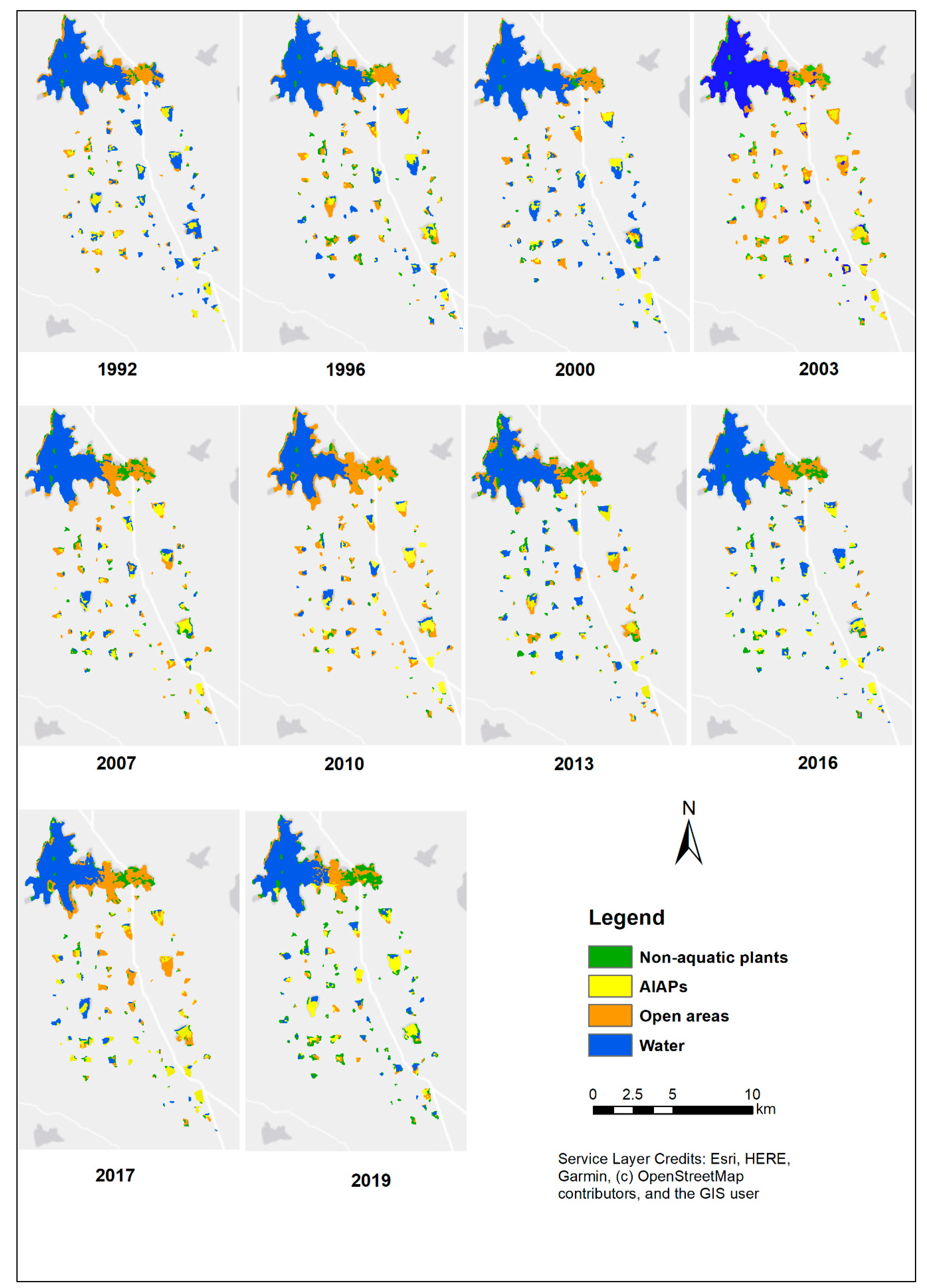
| Non-aquatic plants | 1.060 | 2.388 | 1.277 | 2.522 | 2.995 | 1.379 | 3.387 | 3.279 | 2.477 | 5.575 |
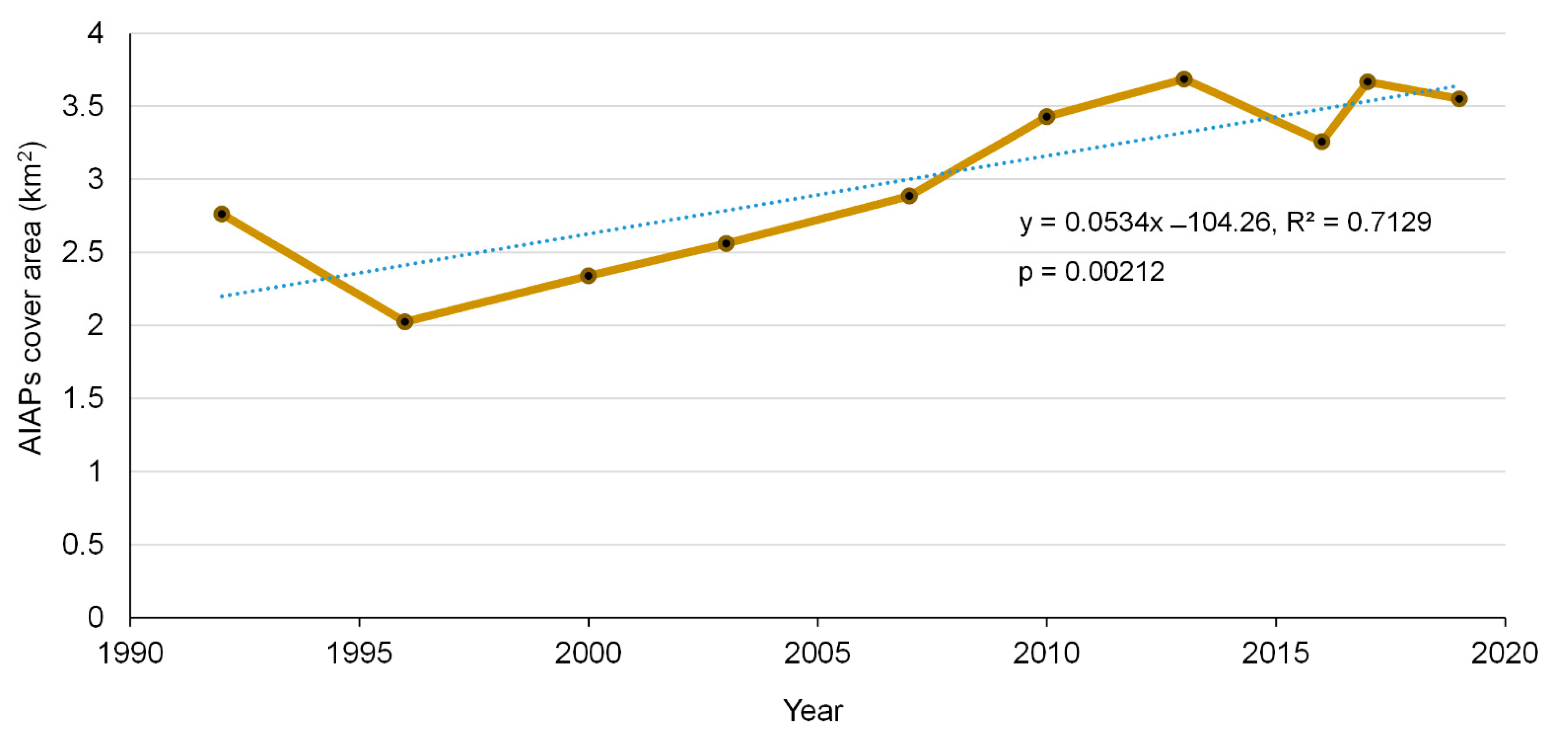
| AIAPs | 2.762 | 2.023 | 2.339 | 2.561 | 2.887 | 3.429 | 3.687 | 3.258 | 3.670 | 3.551 |
| Open areas | 5.340 | 6.303 | 4.812 | 8.100 | 7.351 | 10.323 | 4.190 | 4.967 | 8.571 | 4.751 |
| Water | 17.190 | 15.639 | 17.925 | 13.170 | 13.119 | 11.223 | 15.089 | 14.850 | 11.635 | 12.476 |
| Total | 26.353 | 26.353 | 26.353 | 26.353 | 26.352 | 26.353 | 26.353 | 26.354 | 26.353 | 26.353 |
| Period | Change in AIAPs Area (km2) | Rate of Change (% change per year) |
|---|---|---|
| 1992–1996 | −0.74 | −0.18 |
| 1996–2000 | 0.32 | 0.08 |
| 2000–2003 | 0.22 | 0.07 |
| 2003–2007 | 0.33 | 0.08 |
| 2007–2010 | 0.54 | 0.18 |
| 2010–2013 | 0.26 | 0.09 |
| 2013–2016 | −0.43 | −0.14 |
| 2016–2017 | 0.41 | 0.41 |
| 2017–2019 | −0.12 | −0.06 |
| 1992–2019 (overall) | 0.79 (28.6% increase) | 0.03 |
| Series/Test | Kendall’s Tau | p-Value | Sen’s Slope |
|---|---|---|---|
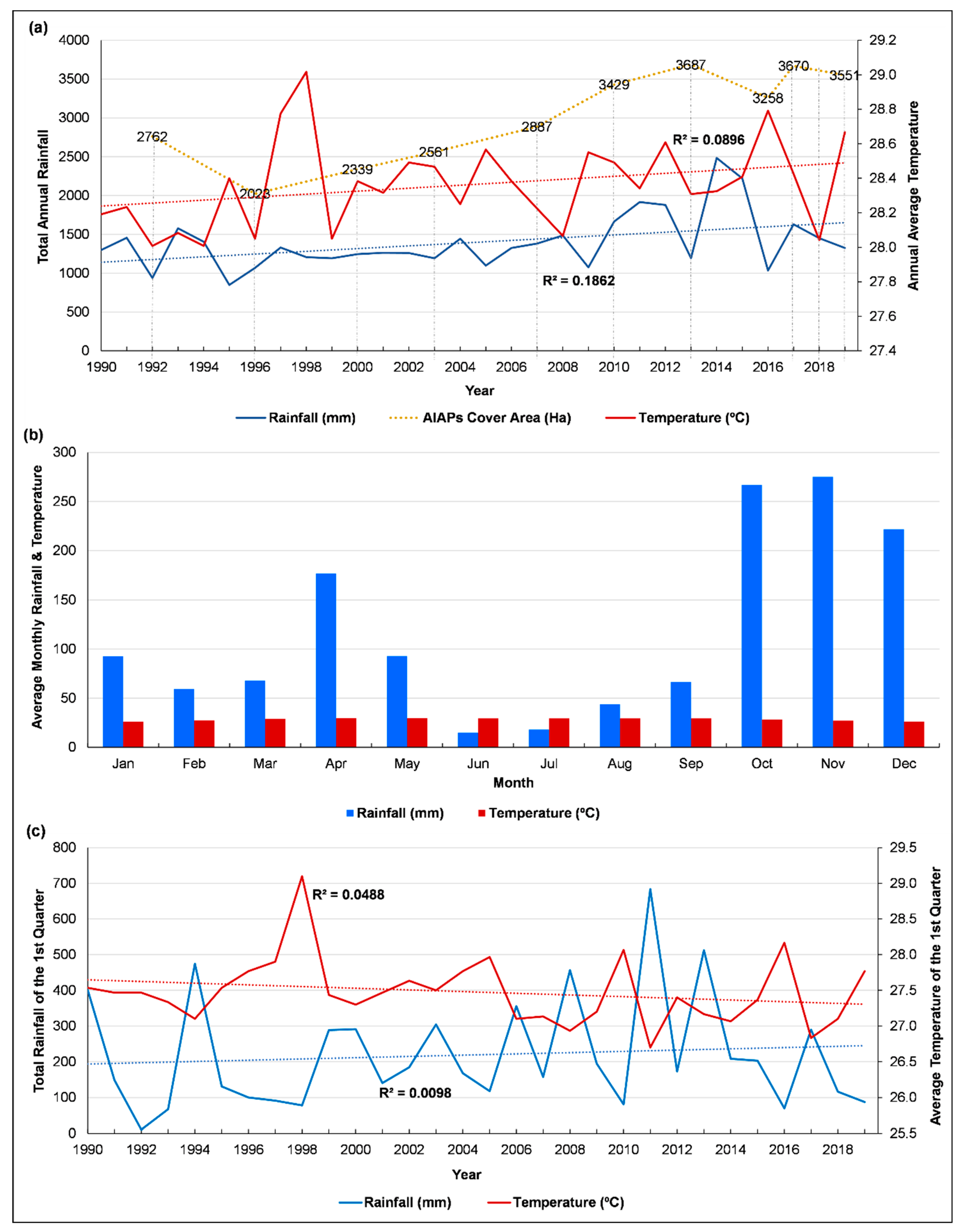
| Annual Average Temperature | 0.253 | 0.050 | 0.012 |
| Total Annual Rainfall | 0.246 | 0.056 | 14.725 |
Publisher’s Note: MDPI stays neutral with regard to jurisdictional claims in published maps and institutional affiliations. |
© 2021 by the authors. Licensee MDPI, Basel, Switzerland. This article is an open access article distributed under the terms and conditions of the Creative Commons Attribution (CC BY) license (http://creativecommons.org/licenses/by/4.0/).
Share and Cite
Kariyawasam, C.S.; Kumar, L.; Kogo, B.K.; Ratnayake, S.S. Long-Term Changes of Aquatic Invasive Plants and Implications for Future Distribution: A Case Study Using a Tank Cascade System in Sri Lanka. Climate 2021, 9, 31. https://0-doi-org.brum.beds.ac.uk/10.3390/cli9020031
Kariyawasam CS, Kumar L, Kogo BK, Ratnayake SS. Long-Term Changes of Aquatic Invasive Plants and Implications for Future Distribution: A Case Study Using a Tank Cascade System in Sri Lanka. Climate. 2021; 9(2):31. https://0-doi-org.brum.beds.ac.uk/10.3390/cli9020031
Chicago/Turabian StyleKariyawasam, Champika S., Lalit Kumar, Benjamin Kipkemboi Kogo, and Sujith S. Ratnayake. 2021. "Long-Term Changes of Aquatic Invasive Plants and Implications for Future Distribution: A Case Study Using a Tank Cascade System in Sri Lanka" Climate 9, no. 2: 31. https://0-doi-org.brum.beds.ac.uk/10.3390/cli9020031