Sensitivity of Simulations of Zambian Heavy Rainfall Events to the Atmospheric Boundary Layer Schemes

 ,
,  , , ,
, , ,
Abstract
:1. Introduction
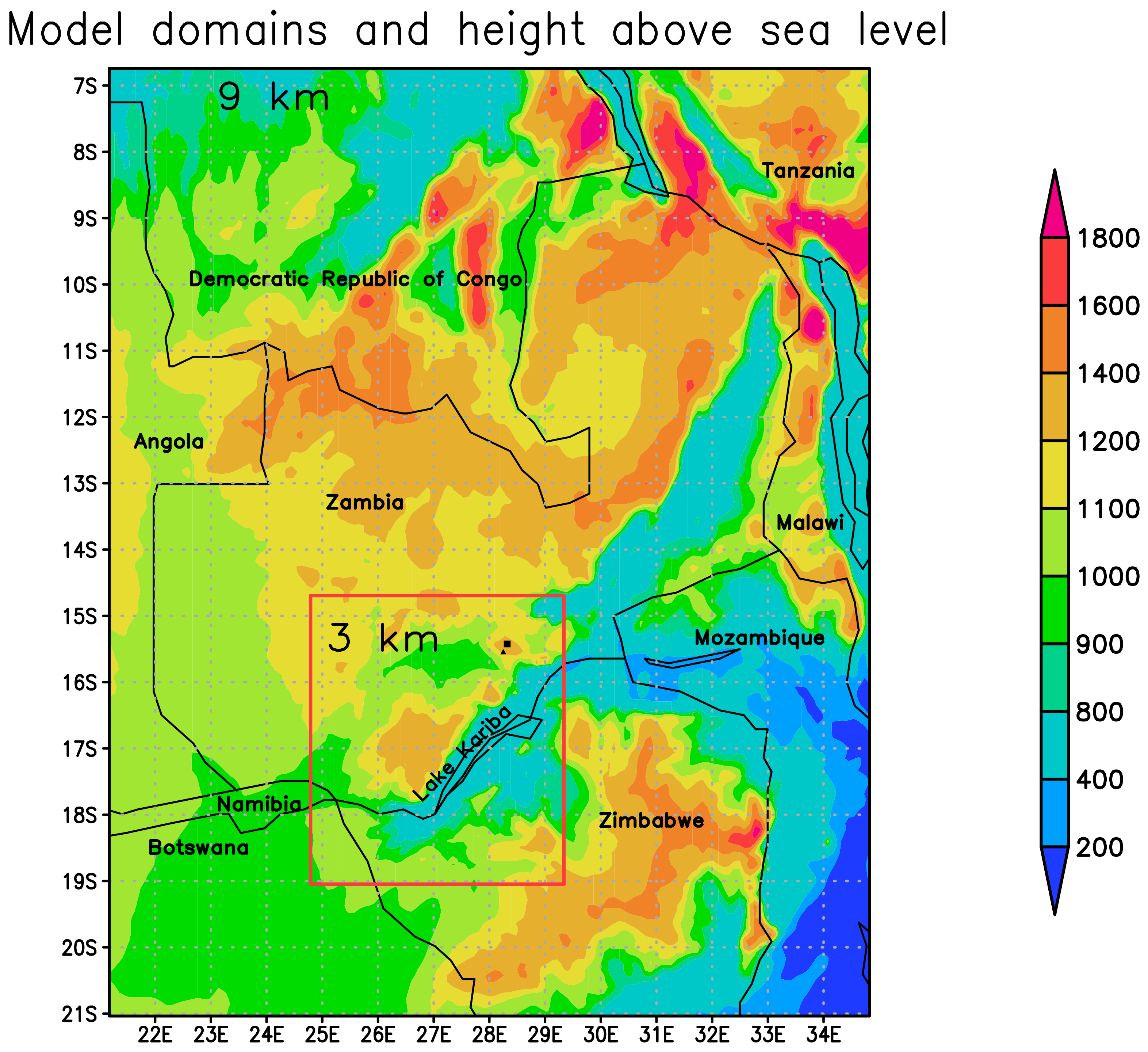
2. Study Area
3. Model, Data and Simulations
3.1. Boundary Layer Schemes
- The Mellor–Yamada–Nakanishi–Niino (MYNN) PBL scheme [26]: this scheme is the improved Mellor–Yamada scheme based on TKE.
- The Community Atmosphere Model (CAM) University of Washington (UW) Moist Turbulence scheme [50]: this scheme is TKE based and also considers shallow convection.
- The Medium Range Forecast (MRF) Model PBL scheme [51]: this scheme includes a non-local term.
- The Yonsei University (YSU) PBL scheme [25]: this scheme includes a diagnostic non-local term, and considers shallow convection, along with a top-down turbulence contribution associated with cloud-top radiative cooling.
3.2. Simulation Design
3.3. Datasets
3.4. Verification Scores
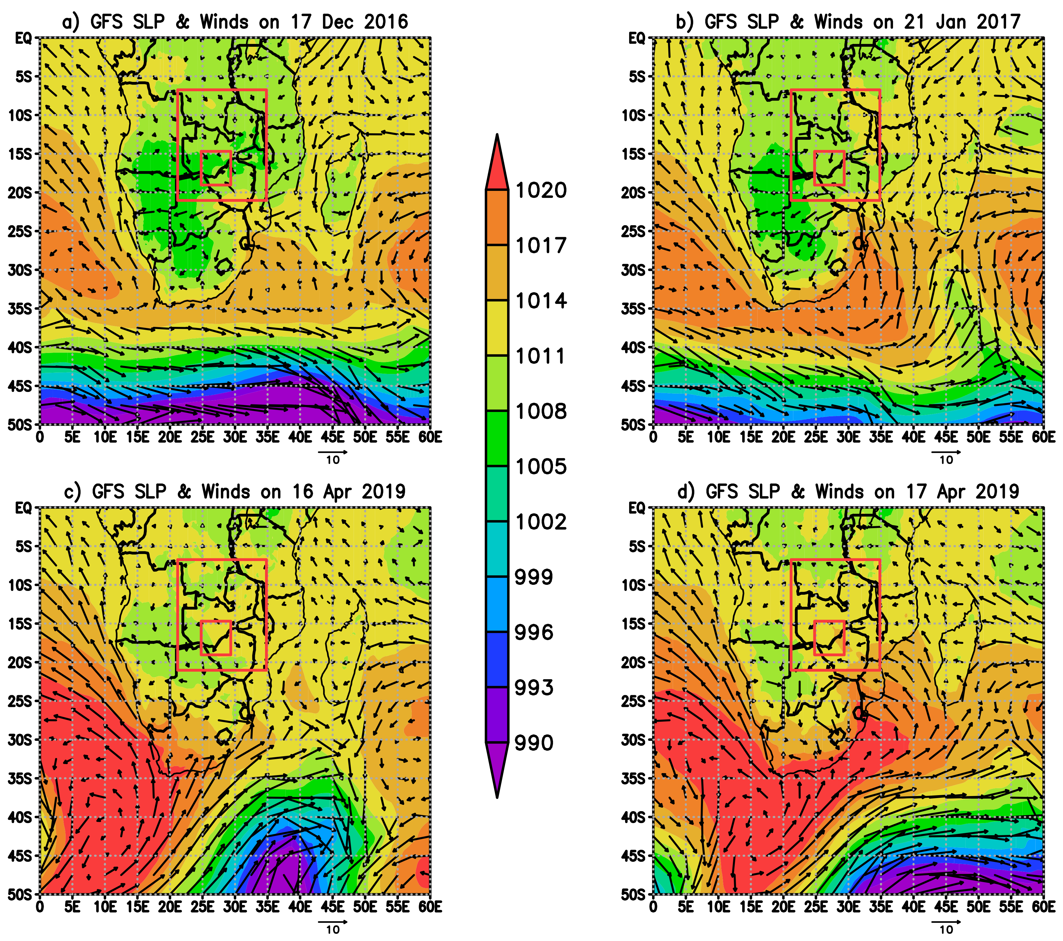
4. Event Descriptions
5. Comparison of Simulations
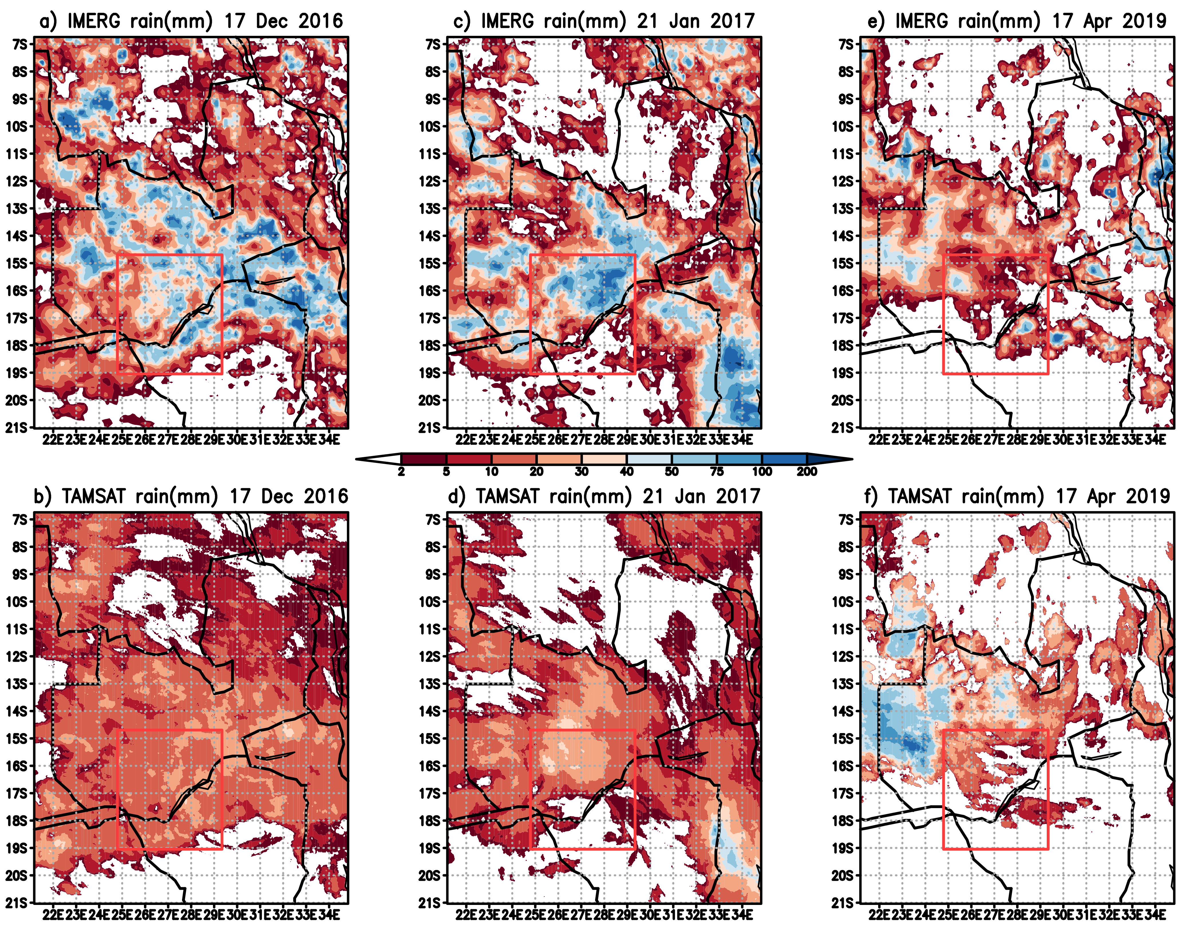
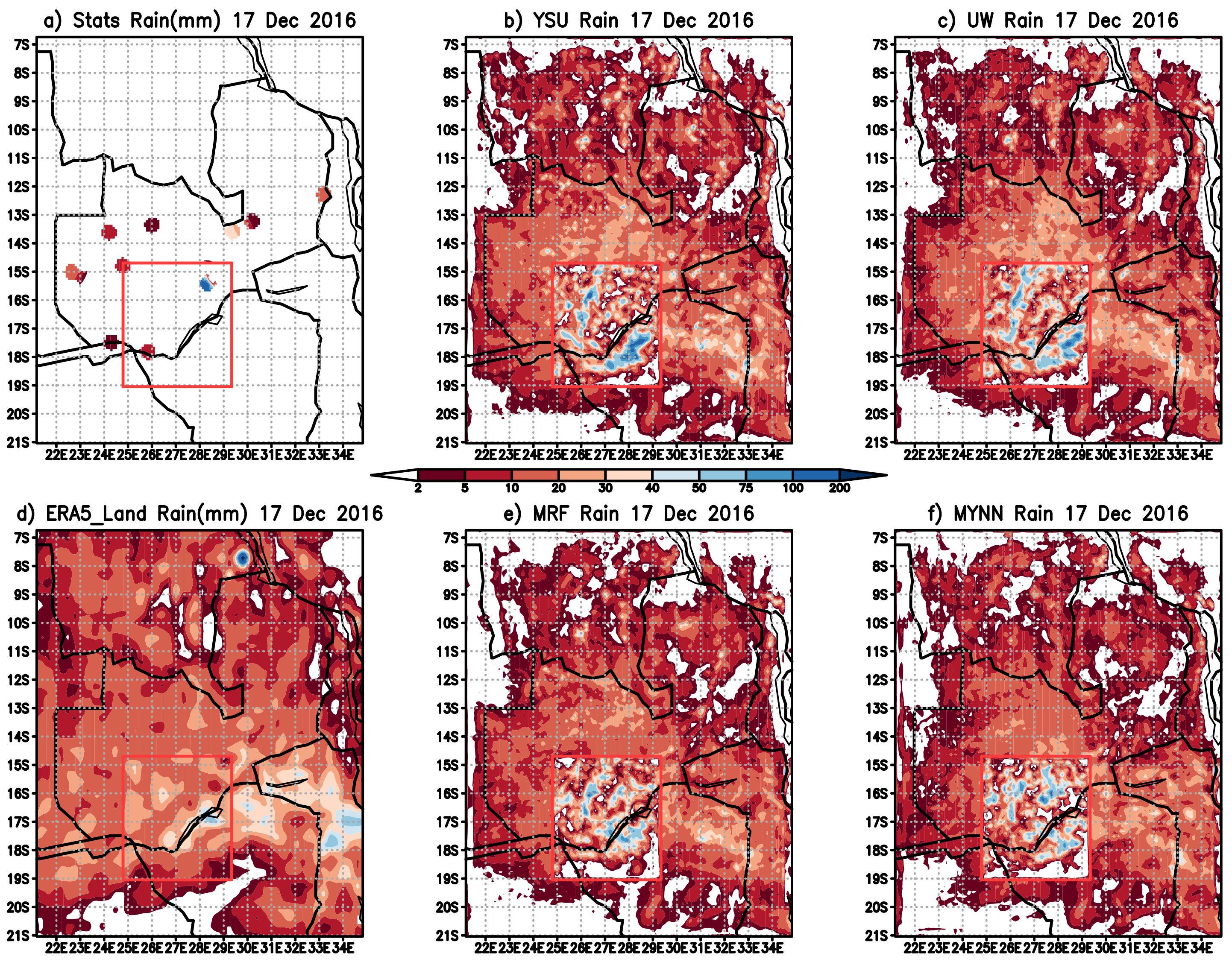
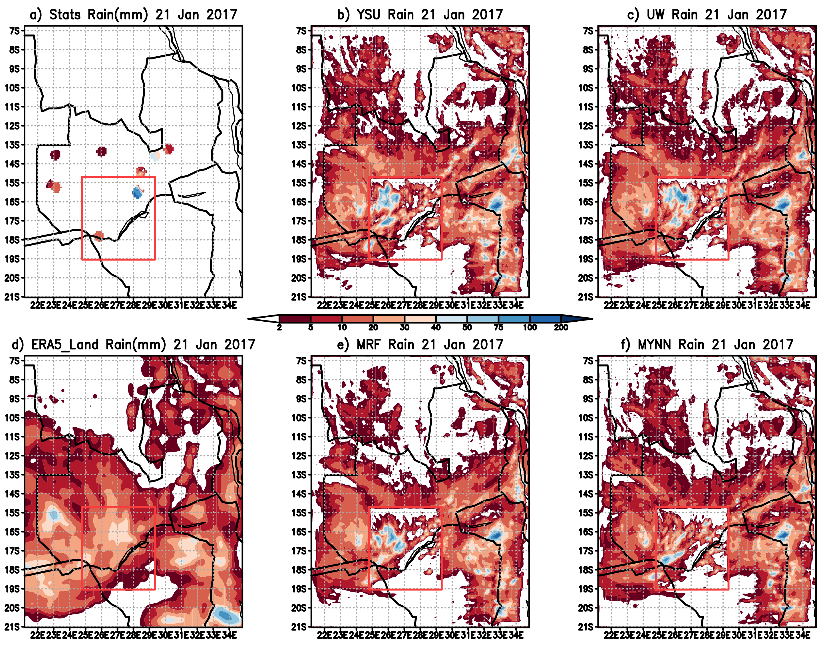
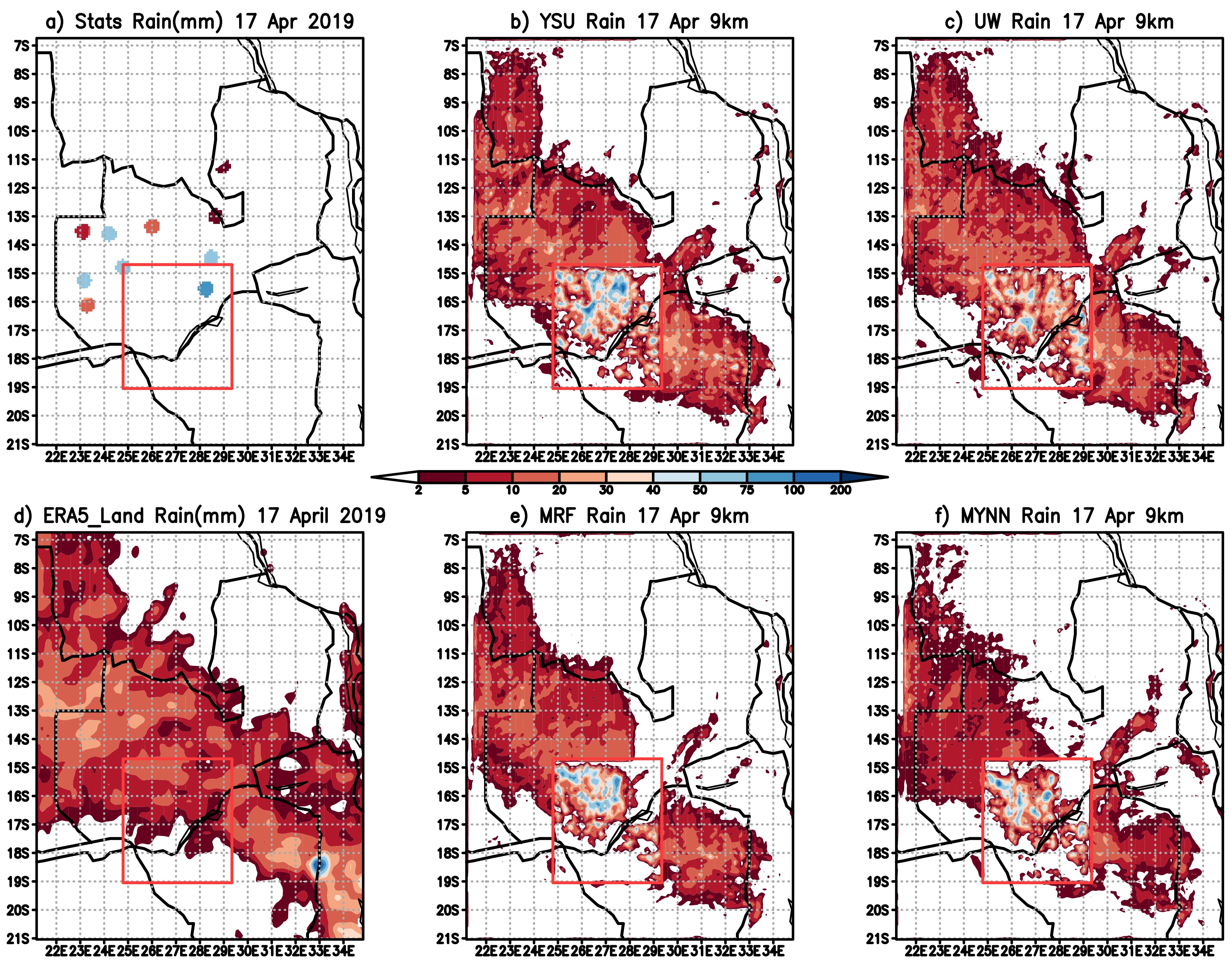
5.1. Twenty-Four Rainfall Eyeball Comparisons
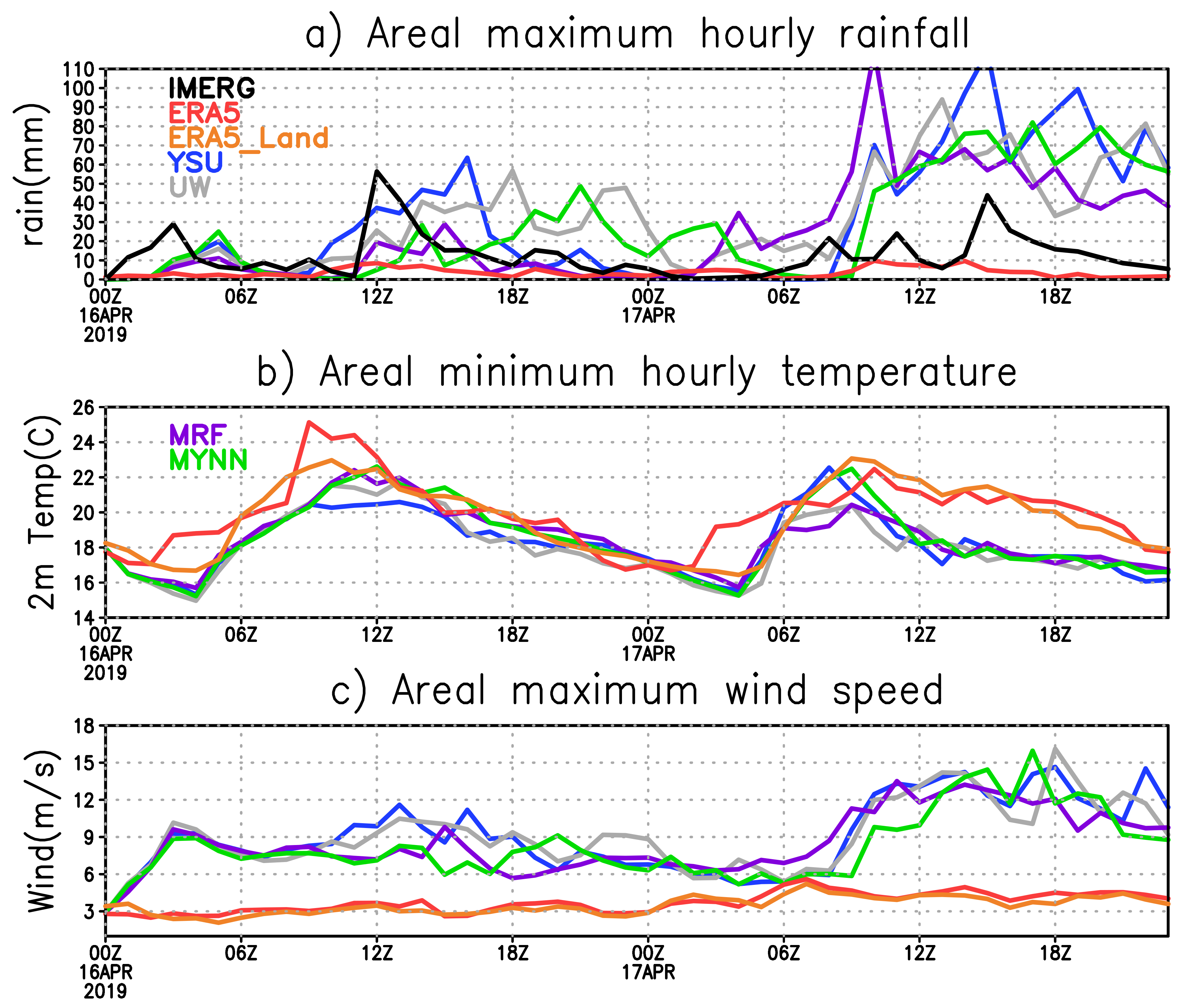
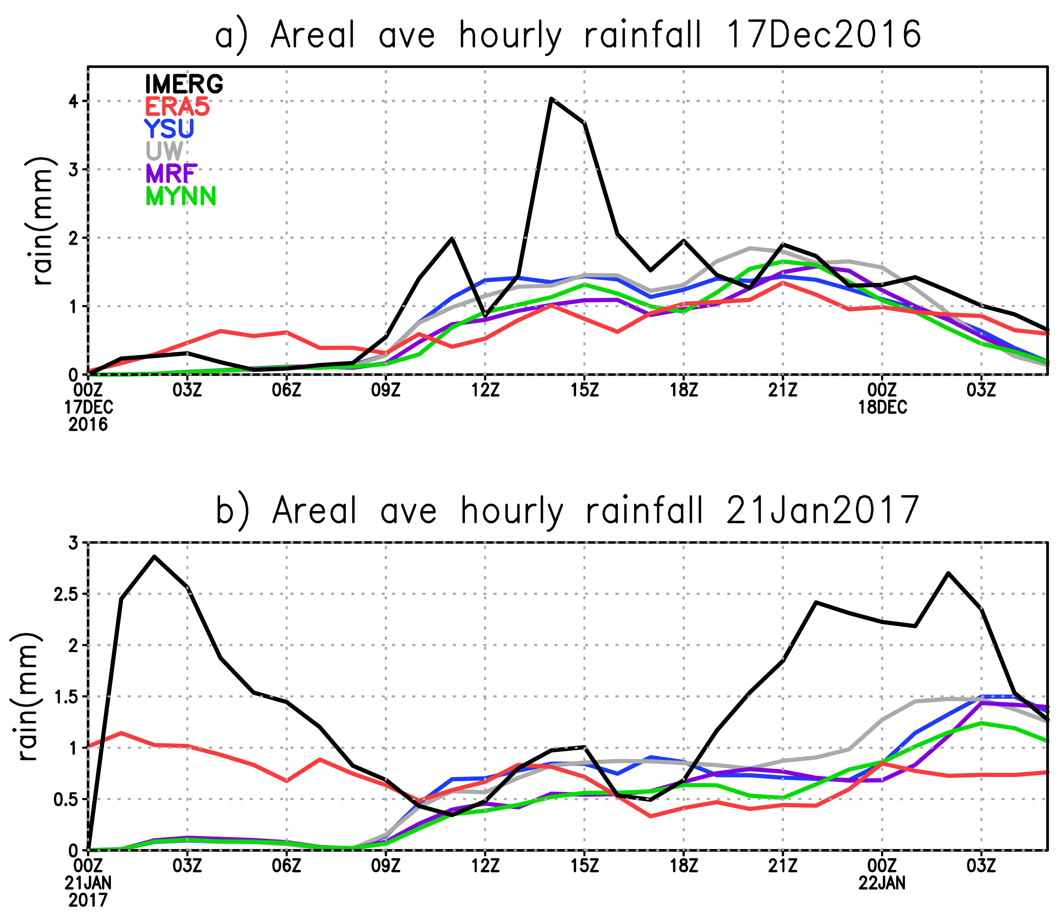
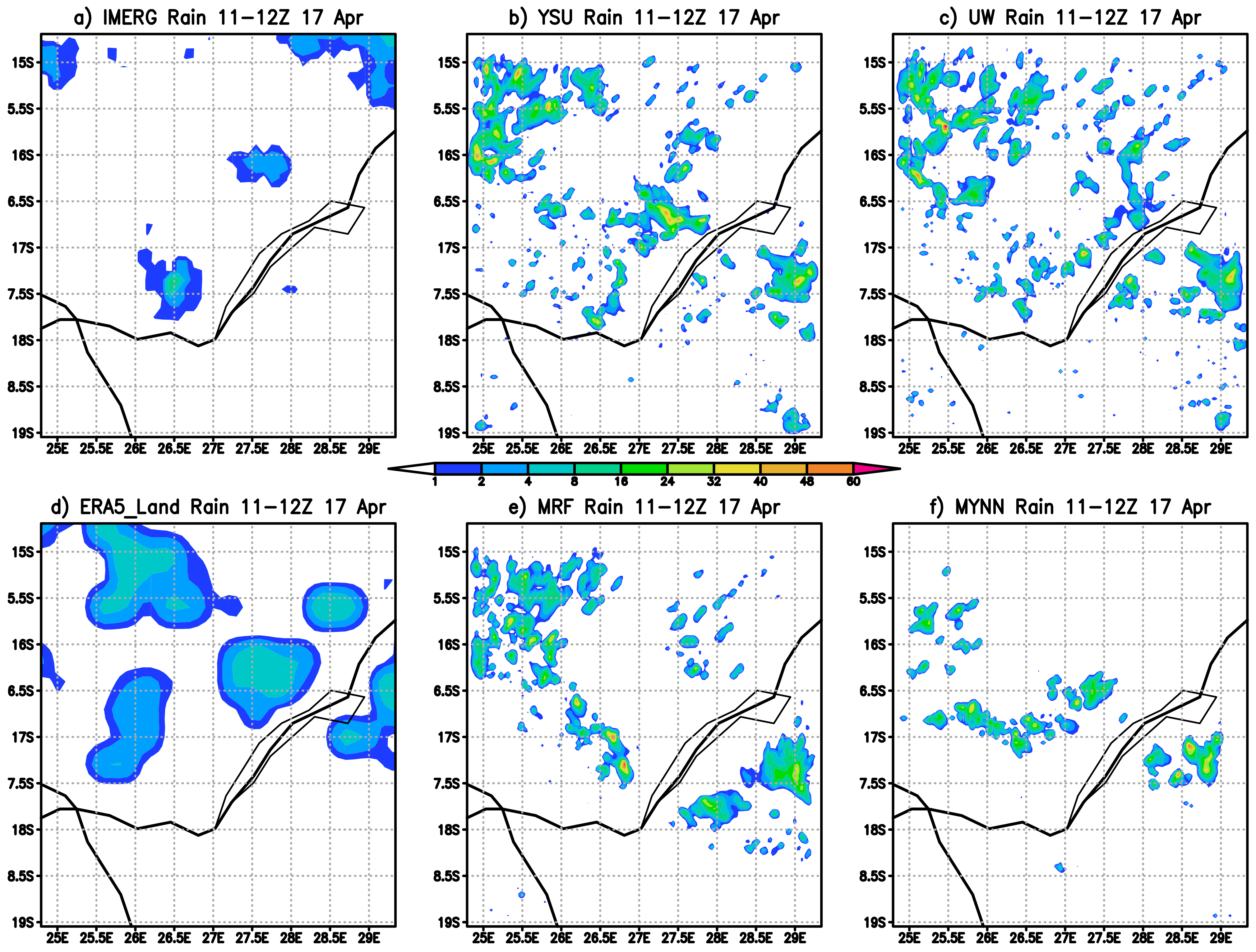
5.2. Hourly Rainfall Eyeball Comparisons
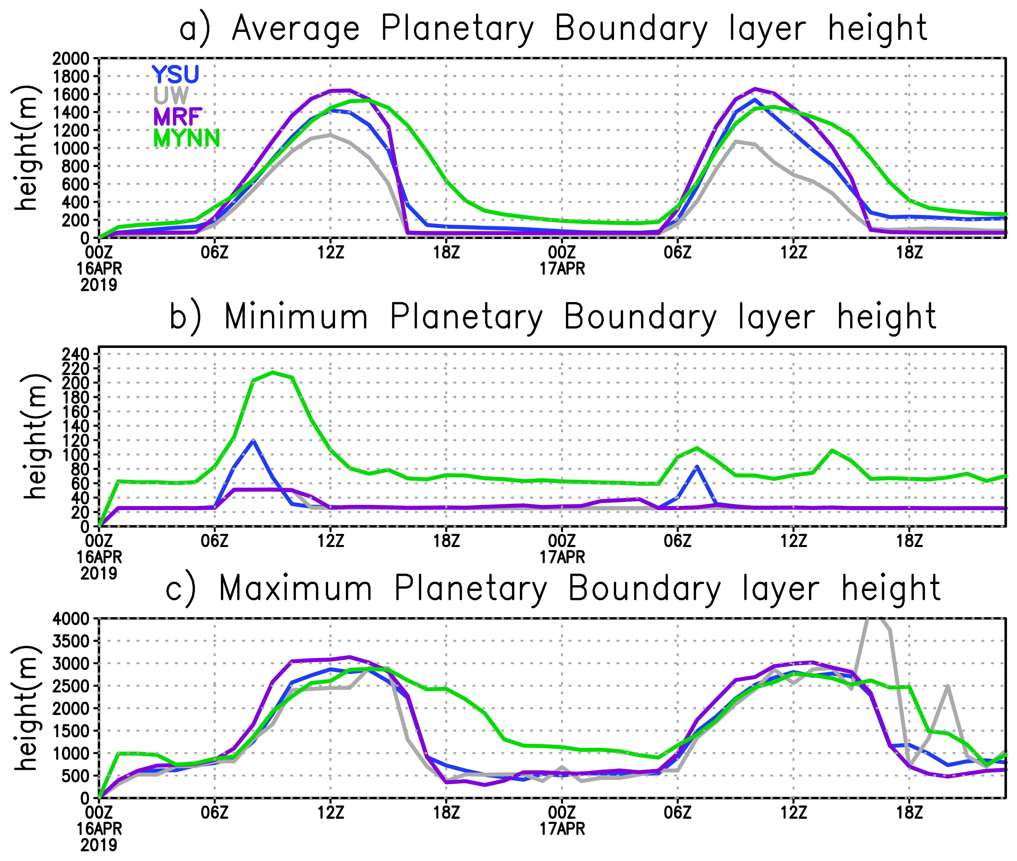
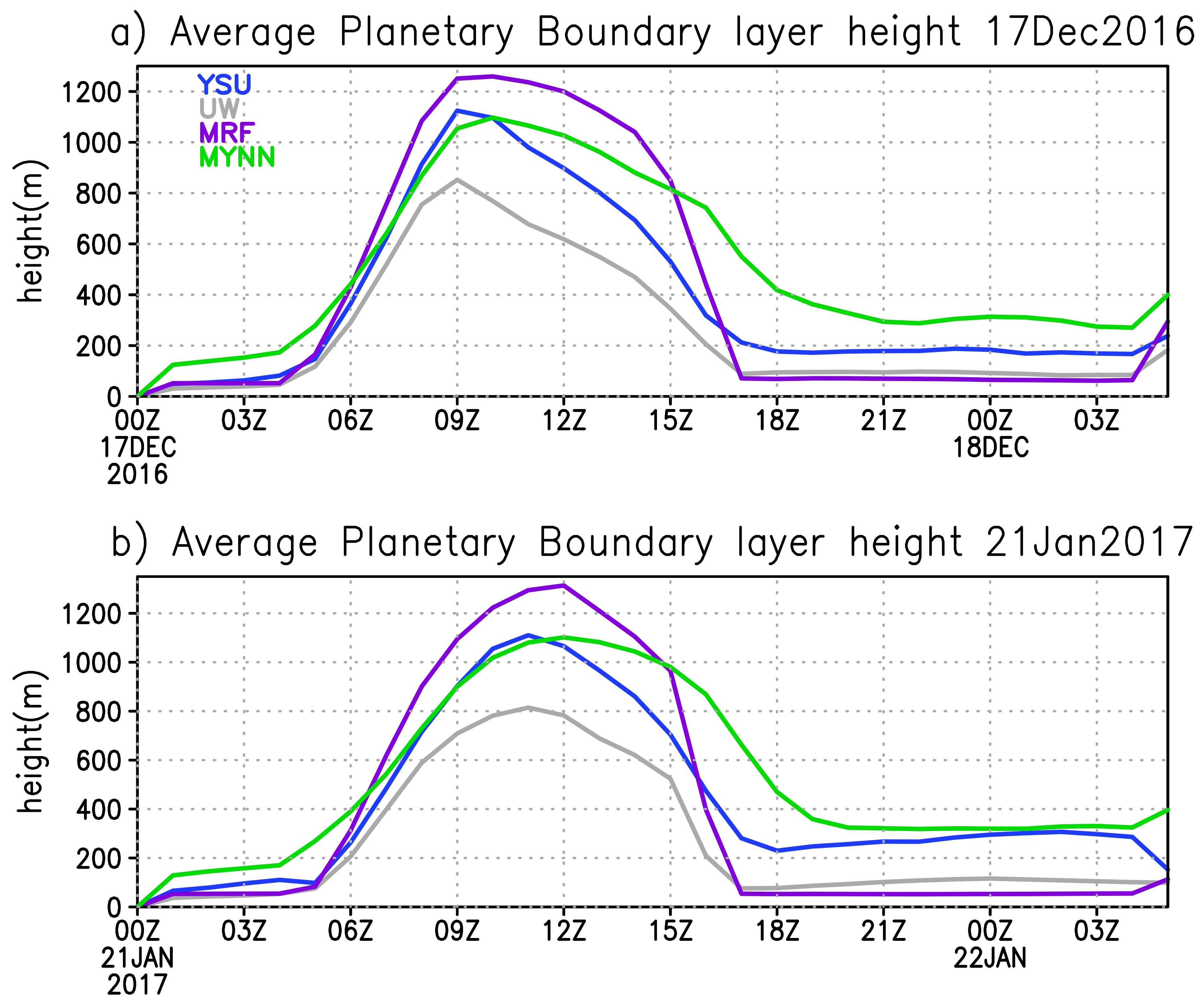
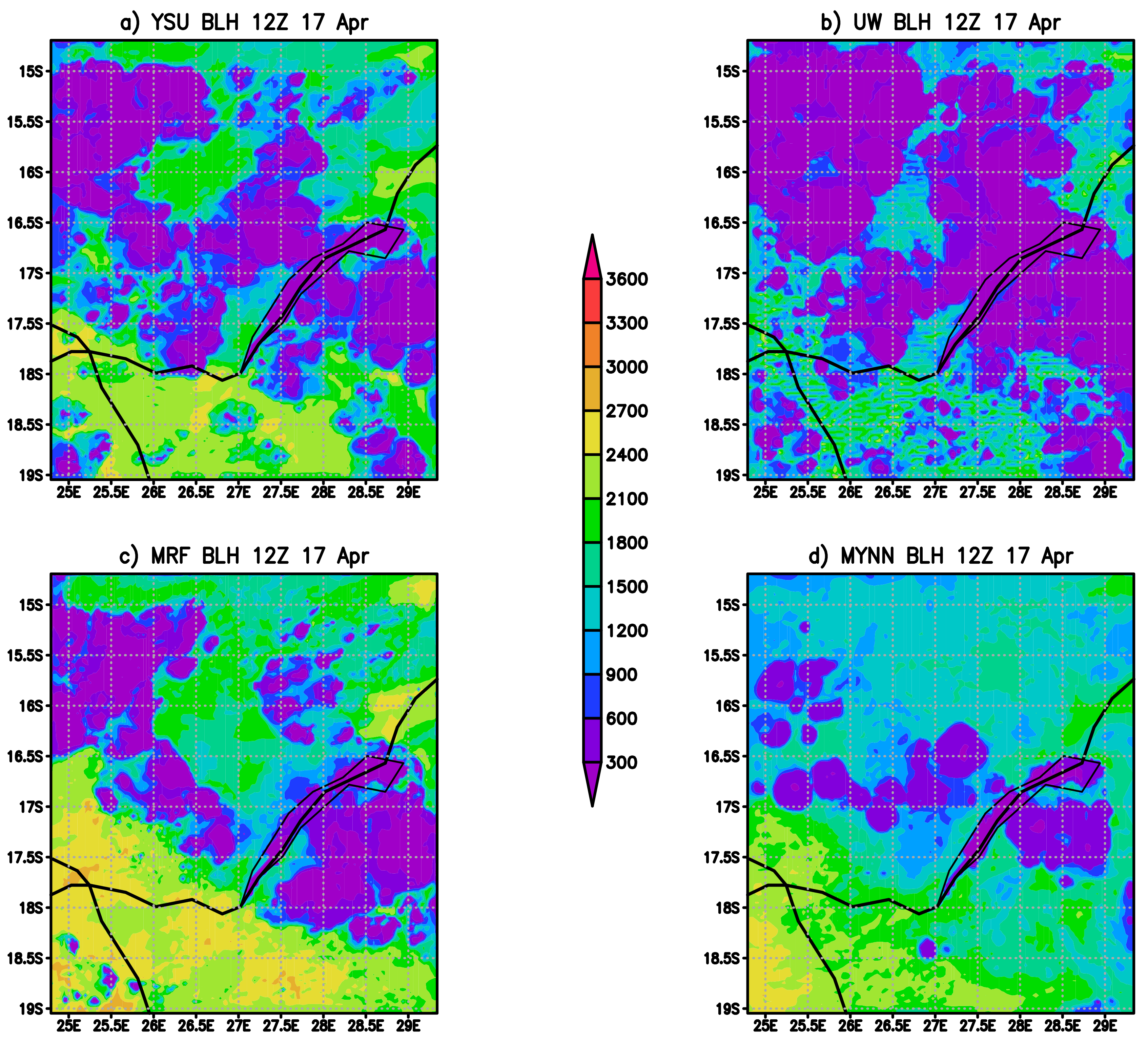
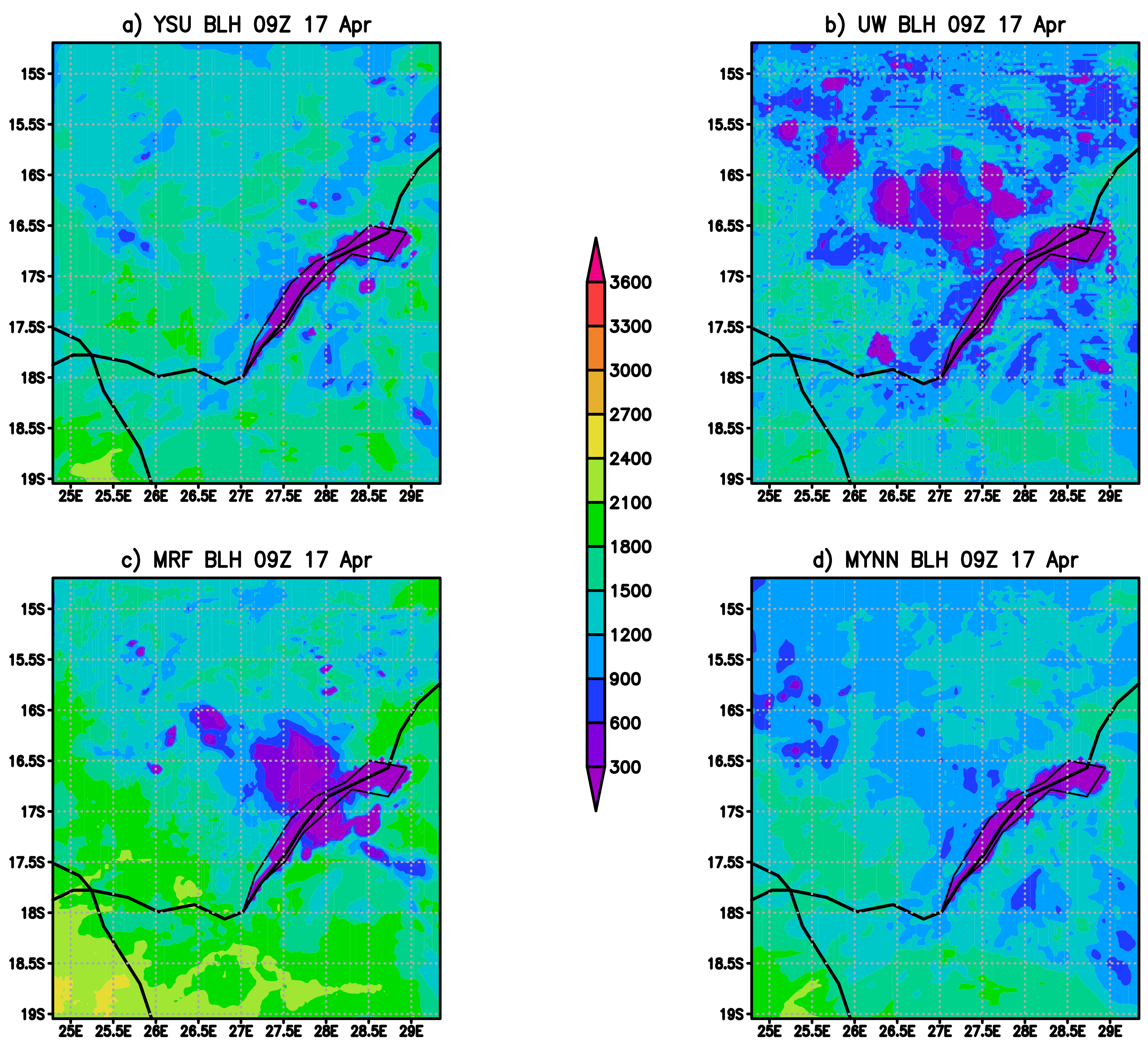
5.3. The Planetary Boundary Layer Height
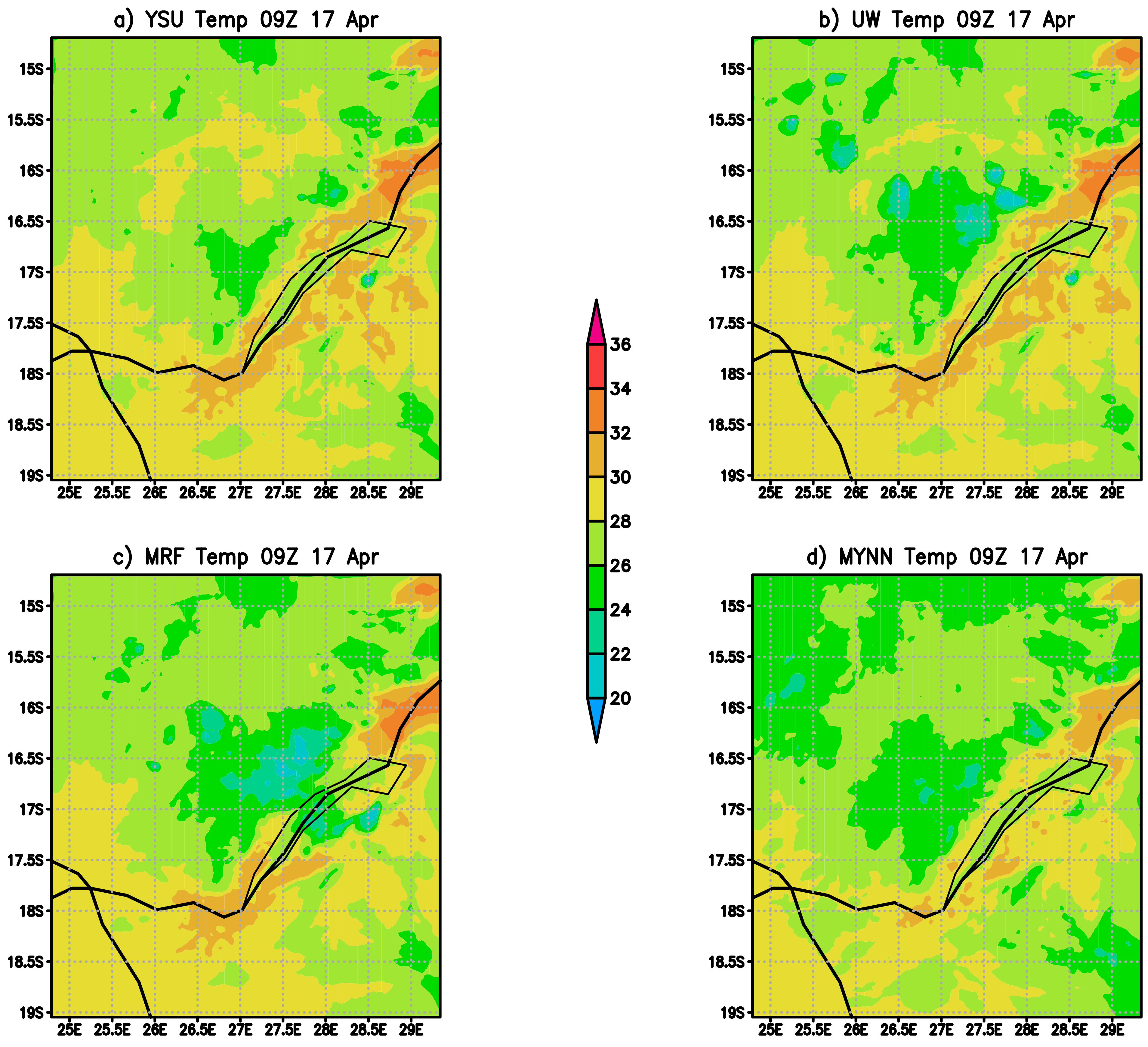
5.4. Near-Surface Temperatures
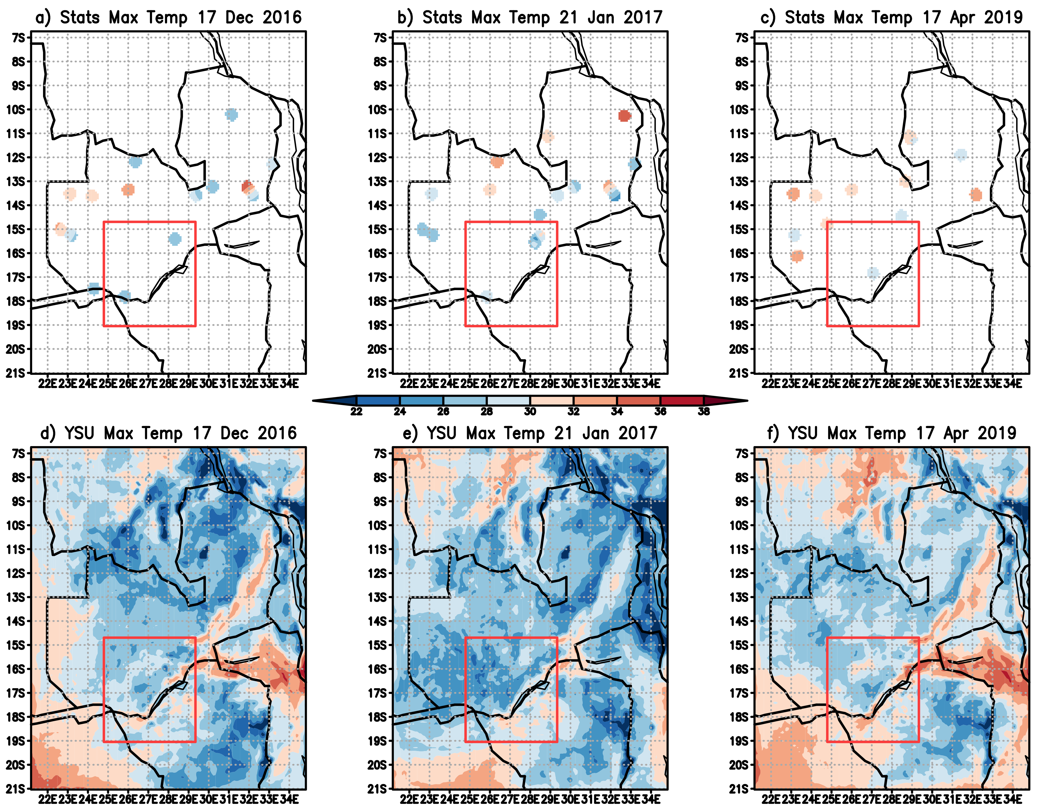
5.5. Verification Statistics
6. Summary and Conclusions
Author Contributions
Funding
Institutional Review Board Statement
Informed Consent Statement
Data Availability Statement
Acknowledgments
Conflicts of Interest
References
- Centre for Research on the Epidemiology of Disasters. The Human Cost of Weather Related Disasters 1995–2015; The United Nations Office for Disaster Risk Reduction, United Nations: Geneva, Switzerland, 2015; pp. 1–27. [Google Scholar]
- World Meteorological Organization (WMO). State of the Climate in Africa 2019; WMO: Geneva, Switzerland, 2020; Volume 1253, pp. 1–35. [Google Scholar]
- United States Agency International Development (USAID). Climate Change Adaptation in Zambia; USAID: Washington, DC, USA, 2020; pp. 1–4.
- Venäläinen, A.; Pilli-Sihvola, K.; Tuomenvirta, H.; Ruuhela, R.; Kululanga, E.; Mtilatila, L.; Kanyanga, J.K.; Nkomoki, J. Analysis of the meteorological capacity for early warnings in Malawi and Zambia. Clim. Dev. 2015, 8, 1–7. [Google Scholar] [CrossRef]
- Skamarock, W.C.; Klemp, J.B.; Dudhia, J.; Gill, D.O.; Liu, Z.; Berner, J.; Wang, W.; Powers, J.G.; Duda, M.G.; Barker, D.M.; et al. A Description of the Advanced Research WRF Version 4; Technical Report; NCAR; NCAR Tech. Note NCAR/TN-556+STR; National Center for Atmospheric Research: Boulder, CO, USA, 2019; p. 145. [CrossRef]
- Courtier, P.; Geleyn, J.F. A global numerical weather prediction model with variable resolution: Application to the shallow model equations. Q. J. R. Meteorol. Soc. 1988, 114, 1321–1346. [Google Scholar] [CrossRef]
- Walters, D.; Baran, A.J.; Boutle, I.; Brooks, M.; Earnshaw, P.; Edwards, J.; Furtado, K.; Hill, P.; Lock, A.; Manners, J.; et al. The Met Office Unified Model Global Atmosphere 7.0/7.1 and JULES Global Land 7.0 configurations. Geosci. Model Devel. 2019, 12, 1909–1963. [Google Scholar] [CrossRef] [Green Version]
- Sela, J. Implementation of the sigma pressure hybrid coordinate into GFS. NCEP Off. Note 2009, 461, 1–25. [Google Scholar]
- ECMWF. IFS Documentation CY47R1; Technical Report; ECMWF: Reading, UK, 2020. [Google Scholar]
- Maidment, R.I.; Grimes, D.I.F.; Black, E.; Tarnavsky, E.; Young, M.; Greatrex, H.; Allan, R.P.; Stein, T.H.M.; Nkonde, E.; Senkunda, S.; et al. A new, long-term daily satellite-based rainfall dataset for operational monitoring in Africa. Nat. Sci. Data 2017, 4, 170063. [Google Scholar] [CrossRef] [PubMed]
- World Meteorological Organization (WMO). Commission for Basic Systems Severe Weather Forecasting Demonstration Project (SWFDP): The Overall Project Plan; Technical Report; WMO: Geneva, Switzerland, 2010. [Google Scholar]
- World Meteorological Organization (WMO). World Weather Information Service: Official Forecasts; WMO: Geneva, Switzerland, 2020; Volume 49, pp. 59–71. [Google Scholar]
- Bauer, P.; Thorpe, A.; Brunet, G. The quiet revolution of numerical weather prediction. Nature 2015, 525, 47–55. [Google Scholar] [CrossRef]
- Carr, H. Atos Supercomputer to Enhance Weather Prediction Capabilities for Leading European Numerical Weather Centre ECMWF; ECMWF: Reading, UK, 2020; pp. 1–3. [Google Scholar]
- Met Office Press Office. Up to £1.2 Billion for Weather and Climate Supercomputer; Met Office: Devon, UK, 2020. [Google Scholar]
- Motshegwa, T.; Wright, C.; Sithole, H.; Ngolwe, C.; Morgan, A. Developing a Cyber-infrastructure for Enhancing Regional Collaboration on Education, Research, Science, Technology and Innovation. In Proceedings of the 2018 IST-Africa Week Conference (IST-Africa), Gaborone, Botswana, 9–11 May 2018; pp. 1–9. [Google Scholar]
- Bopape, M.M.; Sithole, H.; Motshegwa, T.; Rakate, E.; Engelbrecht, F.; Morgan, A.; Ndimeni, L.; Botai, O.J. A Regional Project in Support of the SADC Cyber-Infrastructure Framework Implementation: Weather and Climate. Data Sci. J. 2019, 18, 34. [Google Scholar] [CrossRef] [Green Version]
- Kanno, H.; Sakurai, T.; Shinjo, H.; Miyazaki, H.; Ishimoto, Y.; Saeki, T.; UMETSU, C. Analysis of Meteorological Measurements made over Three Rainy Seasons and Rainfall Simulations in Sinazongwe District, Southern Province, Zambia. Jpn. Agric. Res. Q. 2015, 49, 59–71. [Google Scholar] [CrossRef] [Green Version]
- Stensrud, D. Parameterization Schemes: Keys to Understanding Numerical Weather Prediction Models; Reprint of the 2007 hardback ed.; Cambridge University Press: Cambridge, UK, 2007; p. 480. [Google Scholar] [CrossRef]
- Stull, R.B. An Introduction to Boundary Layer Meteorology; Kluwer Academic Publishers: Dordrecht, The Netherlands, 1988; p. 666. [Google Scholar]
- Houze, R.A.J. Cloud Dynamics; Academic Press: San Diego, CA, USA, 1994; p. 573. [Google Scholar]
- Deardorff, J.W. Parameterization of the planetary boundary layer for use in general circulation models. Mon. Weather. Rev. 1974, 100, 93–106. [Google Scholar] [CrossRef] [Green Version]
- Qian, Y.; Yan, H.; Berg, L.K.; Hagos, S.; Feng, Z.; Yang, B.; Huang, M. Assessing Impacts of PBL and Surface Layer Schemes in Simulating the Surface-Atmosphere Interactions and Precipitation over the Tropical Ocean Using Observations from AMIE/DYNAMO. J. Clim. 2016, 29, 8191–8210. [Google Scholar] [CrossRef]
- Jahn, D.; Gallus, W. Impacts of Modifications to a Local Planetary Boundary Layer Scheme on Forecasts of the Great Plains Low-Level Jet Environment. Weather. Forecast. 2018, 33, 1109–1120. [Google Scholar] [CrossRef]
- Hong, S.Y.; Noh, Y.; Dudhia, J. A New Vertical Diffusion Package with an Explicit Treatment of Entrainment Processes. Mon. Weather. Rev. 2006, 134, 2318–2341. [Google Scholar] [CrossRef] [Green Version]
- Nakanishi, M.; Niino, H. Development of an Improved Turbulence Closure Model for the Atmospheric Boundary Layer. J. Meteorol. Soc. Jpn. 2009, 87, 895–912. [Google Scholar] [CrossRef] [Green Version]
- Bélair, S.; Mailhot, J.; Strapp, J.W.; MacPherson, J.I. An Examination of Local versus Nonlocal Aspects of a TKE-Based Boundary Layer Scheme in Clear Convective Conditions. J. Appl. Meteorol. 1999, 38, 1499–1518. [Google Scholar] [CrossRef]
- Cohen, A.E.; Cavallo, S.M.; Coniglio, M.C.; Brooks, H.E.; Jirak, I.L. Evaluation of Multiple Planetary Boundary Layer Parameterization Schemes in Southeast U.S. Cold Season Severe Thunderstorm Environments. Weather. Forecast. 2017, 32, 1857–1884. [Google Scholar] [CrossRef]
- Comin, A.; Justino, F.; Pezzi, L.; Gurjão, C.; Schumacher, V.; Fernández, A.; Sutil, U. Extreme rainfall event in the Northeast coast of Brazil: A numerical sensitivity study. Meteorol. Atmos. Phys. 2020. [Google Scholar] [CrossRef]
- Hu, X.M.; Nielsen-Gammon, J.W.; Zhang, F. Evaluation of Three Planetary Boundary Layer Schemes in the WRF Model. J. Appl. Meteorol. Climatol. 2010, 49, 1831–1844. [Google Scholar] [CrossRef] [Green Version]
- De Lange, A.; Naidoo, M.; Garland, R.; Dyson, L. Sensitivity of meteorological variables on planetary boundary layer parameterization schemes in the WRF-ARW model. Atmos. Res. 2021, 247, 105214. [Google Scholar] [CrossRef]
- Libanda, B.; Ogwang, B.; Ongoma, V.; Ngonga, C.; Nyasa, L. Diagnosis of the 2010 DJF flood over Zambia. Nat. Hazards 2016, 81, 189–2016. [Google Scholar] [CrossRef]
- Hachigonta, S.; Reason, C. Interannual variability in dry and wet spell characteristics over Zambia. Clim. Res. 2006, 32, 49–62. [Google Scholar] [CrossRef] [Green Version]
- Thurlow, J.; Zhu, T.; Diao, X. The Impact of Climate Variability and Change on Economic Growth and Poverty in Zambia; IFPRI Discussion Papers; International Food Policy Research Institute (IFPRI): Washington, DC, USA, 2009. [Google Scholar]
- Nyambe, S.; Gomes, C.; Lubasi, F.; Gomes, A. Analysis of Lightning Occurence in Zambia. In Proceedings of the 2014 International Conference on Lightning Protection (ICLP), Shanghai, China, 11–18 October 2014; pp. 1919–1925. [Google Scholar] [CrossRef]
- Libanda, B.; Nkolola, N.; Bathsheba, M. Rainfall Variability over Northern Zambia. J. Sci. Res. Rep. 2015, 6, 416–425. [Google Scholar] [CrossRef]
- del Ninno, C.; Marini, A. Household’s vulnerability to shocks in Zambia. Soc. Prot. Discuss. Pap. World Bank 2005, 526, 43. [Google Scholar]
- Luque-Fernandez, M.; Bauernfeind, A.; Díaz, J.; Linares, C.; Omeiri, N.; Guibert, D. Influence of temperature and rainfall on the evolution of cholera epidemics in Lusaka, Zambia, 2003–2006: Analysis of a time series. Trans. R. Soc. Trop. Med. Hyg. 2008, 103, 137–143. [Google Scholar] [CrossRef] [PubMed] [Green Version]
- Chinowsky, P.; Schweikert, A.; Strzepek, N.; Strzepek, K. Infrastructure and climate change: A study of impacts and adaptations in Malawi, Mozambique, and Zambia. Clim. Chang. 2015, 130, 49–62. [Google Scholar] [CrossRef] [Green Version]
- Thurlow, J.; Diao, X. Current Climate Variability and Future Climate Change: Estimated Growth and Poverty Impacts for Zambia. Rev. Dev. Econ. 2012, 16, 394–411. [Google Scholar] [CrossRef] [Green Version]
- Clark, P.; Roberts, N.; Lean, H.; Ballard, S.; Charlton-Perez, C. Convection-permitting models: A step-change in rainfall forecasting. Meteorol. Appl. 2016, 23, 165–181. [Google Scholar] [CrossRef] [Green Version]
- Wang, W. WRF: More Runtime Options. In WRF Tutorial; UNSW: Sydney, NSW, Australia, 2017; p. 46. [Google Scholar]
- Sun, B.Y.; Bi, X. Validation for a tropical belt version of WRF: Sensitivity tests on radiation and cumulus convection parameterizations. Atmos. Ocean. Sci. Lett. 2019, 12, 192–200. [Google Scholar] [CrossRef] [Green Version]
- Iacono, M.; Delamere, J.; Mlawer, E.; Shepard, M.; Clough, S.; Collins, W. Radiative Forcing by Long-Lived Greenhouse Gases: Calculations with the AER Radiative Transfer Models. J. Geophys. Res. 2008, 113. [Google Scholar] [CrossRef]
- Hong, S.Y.; Kim, J.H.; Lim, J.O.; Dudhia, J. The WRF single moment microphysics scheme (WSM). J. Korean Meteorol. Soc. 2006, 42, 129–151. [Google Scholar]
- Tiedtke, M.A. A Comprehensive Mass Flux Scheme For Cumulus Parameterization In Large-Scale Models. Mon. Weather. Rev. 1989, 117, 1779–1800. [Google Scholar] [CrossRef] [Green Version]
- Zhang, C.; Wang, Y.; Hamilton, K. Improved Representation of Boundary Layer Clouds over the Southeast Pacific in ARW-WRF Using a Modified Tiedtke Cumulus Parameterization Scheme. Mon. Weather Rev. 2011, 139, 3489–3513. [Google Scholar] [CrossRef] [Green Version]
- Zhang, S.; Matsui, T.; Cheung, S.; Zupanski, M.; Peters-Lidard, C. Impact of Assimilated Precipitation-Sensitive Radiances on the NU-WRF Simulation of the West African Monsoon. Mon. Weather Rev. 2017, 145, 3881–3900. [Google Scholar] [CrossRef]
- Holtslag, A.A.M.; Boville, B.A. Local Versus Nonlocal Boundary-Layer Diffusion in a Global Climate Model. J. Clim. 1993, 6, 1825–1842. [Google Scholar] [CrossRef] [Green Version]
- Bretherton, C.S.; Park, S. A New Moist Turbulence Parameterization in the Community Atmosphere Model. J. Clim. 2009, 22, 3422–3448. [Google Scholar] [CrossRef]
- Hong, S.Y.; Pan, H.L. Nonlocal Boundary Layer Vertical Diffusion in a Medium-Range Forecast Model. Mon. Weather Rev. 1996, 124, 2322–2339. [Google Scholar] [CrossRef] [Green Version]
- Lean, H.W.; Clark, P.A.; Dixon, M.; Roberts, N.M.; Fitch, A.; Forbes, R.; Halliwell, C. Characteristics of High-Resolution Versions of the Met Office Unified Model for Forecasting Convection over the United Kingdom. Mon. Weather Rev. 2008, 136, 3408–3424. [Google Scholar] [CrossRef]
- Kain, J.S.; Weiss, S.J.; Levit, J.J.; Baldwin, M.E.; Bright, D.R. Examination of convection-allowing configurations of the WRF model for the prediction of severe convective weather: The SPC/NSSL Spring Program 2004. Wea. Forecast. 2006, 21, 167–181. [Google Scholar] [CrossRef] [Green Version]
- Crook, J.; Klein, C.; Folwell, S.; Taylor, C.M.; Parker, D.J.; Stratton, R.; Stein, T. Assessment of the Representation of West African Storm Lifecycles in Convection-Permitting Simulations. Earth Space Sci. 2019, 6, 818–835. [Google Scholar] [CrossRef] [Green Version]
- Tarnavsky, E.; Grimes, D.; Maidment, R.; Black, E.; Allan, R.; Stringer, M.; Chadwick, R.; Kayitakire, F. Extension of the TAMSAT Satellite-Based Rainfall Monitoring over Africa and from 1983 to Present. J. Appl. Meteorol. Clim. 2014, 53, 2805–2822. [Google Scholar] [CrossRef] [Green Version]
- Huffman, G.; Bolvin, D.; Braithwaite, D.; Hsu, K.; Joyce, R.; Xie, P. NASA Global Precipitation Measurement Integrated Multi-Satellite Retrievals for GPM (IMERG); Algorithm Theoretical Basis Doc., Version 4.4; NASA’s Precipitation Processing Center; NASA: Washington, DC, USA, 2014; Volume 5, 30p.
- Hersbach, H.; Dee, D. ERA5 Reanalysis Is in Production; ECMWF: Reading, UK, 2016; p. 147. [Google Scholar]
- Davis, C.; Brown, B.; Bullock, R. Object-Based Verification of Precipitation Forecasts. Part I: Methodology and Application to Mesoscale Rain Areas. Mon. Weather. Rev. 2006, 134, 1772–1784. [Google Scholar] [CrossRef] [Green Version]
- Davis, C.; Brown, B.; Bullock, R. Object-Based Verification of Precipitation Forecasts. Part II: Application to Convective Rain Systems. Mon. Weather. Rev. 2006, 134, 1785–1795. [Google Scholar] [CrossRef] [Green Version]
- Brown, B.; Bullock, R.; Gotway, J.; Ahijevch, D.; Davis, C.; Gilleland, E.; Holland, L. Application of the MODE object-based verification tool for the evaluation of model precipitation fields. In Proceedings of the 22nd Conference on Weather Analysis and Forecasting/18th Conference on Numerical Weather Prediction, Park City, UT, USA, 25 June 2007. [Google Scholar]
- Beusch, L.; Foresti, L.; Gabella, M.; Hamann, U. Satellite-Based Rainfall Retrieval: From Generalized Linear Models to Artificial Neural Networks. Remote. Sens. 2018, 10, 939. [Google Scholar] [CrossRef] [Green Version]
- Kerns, B.; Chen, S. ECMWF and GFS model forecast verification during DYNAMO: Multiscale variability in MJO initiation over the equatorial Indian Ocean. J. Geophys. Res. Atmos. 2014, 119, 3736–3755. [Google Scholar] [CrossRef]
- Dias, J.; Gehne, M.; Kiladis, G.; Sakaeda, N.; Bechtold, P.; Haiden, T. Equatorial Waves and the Skill of NCEP and ECMWF Numerical Weather Prediction Systems. Mon. Weather. Rev. 2018, 146, 1763–1784. [Google Scholar] [CrossRef]
- Molongwane, C.; Bopape, M.J.; Fridlind, A.; Motshegwa, T.; Matsui, T.; Phaduli, E.; Sehurutshi, B.; Maisha, R. Sensitivity of Botswana Ex-Tropical Cyclone Dineo rainfall simulations to cloud microphysics scheme. AAS Open Res. 2020, 3, 30. [Google Scholar] [CrossRef]
- Ndarana, T.; Rammopo Tsholanang, S.; Chikoore, H.; Barnes, M.A.; Bopape, M.J. A quasi-geostrophic diagnosis of the zonal flow associated with cut-off lows over South Africa and surrounding oceans. Clim. Dyn. 2020, 55, 2631–2644. [Google Scholar] [CrossRef]
- Somses, S.; Bopape, M.J.M.; Ndarana, T.; Fridlind, A.; Matsui, T.; Phaduli, E.; Limbo, A.; Maikhudumu, S.; Maisha, R.; Rakate, E. Convection parametrization and multi-nesting dependence of a heavy rainfall event over Namibia with Weather Research and Forecasting (WRF) model. Climate 2020, 8, 112. [Google Scholar] [CrossRef]
- Thorne, V.; Coakeley, P.; Grimes, D.; Dugdale, G. Comparison of TAMSAT and CPC Rainfall Estimates with rainfall, for southern Africa. Int. J. Remote Sens. 2001, 22, 1951–1974. [Google Scholar] [CrossRef]
- Syama, S.; Masocha, M.; Dube, T. Evaluation of TAMSAT satellite rainfall estimates for southern Africa: An inter-product comparison study. Phys. Chem. Earth Parts A/B/C 2019, 112, 141–153. [Google Scholar] [CrossRef]
- Beck, H.; Pan, M.; Roy, T.; Weedon, G.; Pappenberger, F.; van Dijk, A.; Huffman, G.; Adler, R.; Wood, E. Daily evaluation of 26 precipitation datasets using Stage-IV gauge-radar data for the CONUS. Hydrol. Earth Syst. Sci. 2019, 23, 207–224. [Google Scholar] [CrossRef] [Green Version]
- Bopape, M.J.; Engelbrecht, F.; Randall, D.; Landman, W. Simulations of an isolated two-dimensional thunderstorm: Sensitivity to cloud droplet size and the presence of graupel. Asia-Pac. J. Atmos. Sci. 2014, 50, 139–151. [Google Scholar] [CrossRef] [Green Version]
- Champion, A.; Hodges, K. Importance of resolution and model configuration when downscaling extreme precipitation. Tellus A 2014, 66. [Google Scholar] [CrossRef] [Green Version]
- Medeiros, B.; Hall, A.; Stevens, B. What controls the mean depth of the PBL? Earth Space Sci. 2005, 18, 3157–3172. [Google Scholar] [CrossRef] [Green Version]
- Efstathiou, G.A.; Plant, R.S.; Bopape, M.J.M. Simulation of an Evolving Convective Boundary Layer Using a Scale-Dependent Dynamic Smagorinsky Model at Near-Gray-Zone Resolutions. J. Appl. Meteorol. Clim. 2018, 57, 2197–2214. [Google Scholar] [CrossRef]
- Bopape, M.J.; Plant, R.; Coceal, O.; Efstathiou, G.; Valdivieso, M. Effects of stability functions in a dynamic model convective boundary layer simulation. Atmos. Sci. Lett. 2021, 22, e1008. [Google Scholar] [CrossRef]
- Steeneveld, G.J.; Peerlings, E. Mesoscale Model Simulation of a Severe Summer Thunderstorm in The Netherlands: Performance and Uncertainty Assessment for Parameterised and Resolved Convection. Atmosphere 2020, 11, 811. [Google Scholar] [CrossRef]
- Cintineo, R.; Otkin, J.A.; Xue, M.; Kong, F. Evaluating the Performance of Planetary Boundary Layer and Cloud Microphysical Parameterization Schemes in Convection-Permitting Ensemble Forecasts Using Synthetic GOES-13 Satellite Observations. Mon. Weather. Rev. 2014, 142, 163–182. [Google Scholar] [CrossRef] [Green Version]


| Scheme | Non-Local | TKE-Based | Shallow Convection |
|---|---|---|---|
| YSU | Yes | No | Yes |
| UW | No | Yes | Yes |
| MRF | Yes | No | No |
| MYNN | No | Yes | No |
| Observations | |||
|---|---|---|---|
| Yes | No | ||
| Forecast | Yes | hits (H) | false alarms (F) |
| No | misses (M) | correct rejects (R) | |
| 17 December 2016 | |||||
|---|---|---|---|---|---|
| YSU | MRF | MYNN | UW | ||
| Tmax | Bias | −1.32012749 | −1.38775444 | −2.77817154 | −1.38088036 |
| RMSE | 0.486743391 | 0.493839473 | 0.977323115 | 0.588211000 | |
| Tmin | Bias | 1.46163368 | 1.44644737 | 1.04733276 | 1.35207367 |
| RMSE | 0.352237523 | 0.259509355 | 0.141910866 | 0.322271198 | |
| 21 January 2017 | |||||
| YSU | MRF | MYNN | UW | ||
| Tmax | Bias | −2.41129112 | −2.37238693 | −3.80073738 | −2.59328842 |
| RMSE | 1.05125797 | 0.493839473 | 1.18280017 | 1.01926601 | |
| Tmin | Bias | 0.257066727 | −0.03591537 | −0.09047127 | 0.197696686 |
| RMSE | 0.765877962 | 0.259509355 | 0.620617151 | 0.802365541 | |
| 17 April 2019 | |||||
| YSU | MRF | MYNN | UW | ||
| Tmax | Bias | −2.97936249 | −2.92316628 | −4.44790268 | −2.87375450 |
| RMSE | 1.00955522 | 1.01955235 | 1.48482561 | 0.488890052 | |
| Tmin | Bias | 0.302921295 | 0.432020187 | 0.01034927 | 0.177062988 |
| RMSE | 0.603425622 | 0.444622010 | 0.662797749 | 0.645322680 | |
Publisher’s Note: MDPI stays neutral with regard to jurisdictional claims in published maps and institutional affiliations. |
© 2021 by the authors. Licensee MDPI, Basel, Switzerland. This article is an open access article distributed under the terms and conditions of the Creative Commons Attribution (CC BY) license (http://creativecommons.org/licenses/by/4.0/).
Share and Cite
Bopape, M.-J.M.; Waitolo, D.; Plant, R.S.; Phaduli, E.; Nkonde, E.; Simfukwe, H.; Mkandawire, S.; Rakate, E.; Maisha, R. Sensitivity of Simulations of Zambian Heavy Rainfall Events to the Atmospheric Boundary Layer Schemes. Climate 2021, 9, 38. https://0-doi-org.brum.beds.ac.uk/10.3390/cli9020038
Bopape M-JM, Waitolo D, Plant RS, Phaduli E, Nkonde E, Simfukwe H, Mkandawire S, Rakate E, Maisha R. Sensitivity of Simulations of Zambian Heavy Rainfall Events to the Atmospheric Boundary Layer Schemes. Climate. 2021; 9(2):38. https://0-doi-org.brum.beds.ac.uk/10.3390/cli9020038
Chicago/Turabian StyleBopape, Mary-Jane M., David Waitolo, Robert S. Plant, Elelwani Phaduli, Edson Nkonde, Henry Simfukwe, Stein Mkandawire, Edward Rakate, and Robert Maisha. 2021. "Sensitivity of Simulations of Zambian Heavy Rainfall Events to the Atmospheric Boundary Layer Schemes" Climate 9, no. 2: 38. https://0-doi-org.brum.beds.ac.uk/10.3390/cli9020038