The Stationary Concentrated Vortex Model
by
 and
and
Oleg Onishchenko
1,2, 
Viktor Fedun
3,*,
Wendell Horton
4,
Oleg Pokhotelov
1,
Natalia Astafieva
2,
Samuel J. Skirvin
3 and
and
Gary Verth
5 1
Institute of Physics of the Earth, 10 B. Gruzinskaya, 123242 Moscow, Russia
2
Space Research Institute, 84/32 Profsouznaya Str., 117997 Moscow, Russia
3
Plasma Dynamics Group, Department of Automatic Control and Systems Engineering, University of Sheffield, Mappin 6 Str., Sheffield S1 3JD, UK
4
Space and Geophysical Laboratory, Applied Research Laboratory at the University of Texas (ARLUT), Austin, TX 78705, USA
5
Plasma Dynamics Group, School of Mathematics and Statistics, University of Sheffield, Hicks Building, Sheffield S3 7RH, UK
*
Author to whom correspondence should be addressed.
Climate 2021, 9(3), 39; https://0-doi-org.brum.beds.ac.uk/10.3390/cli9030039
Submission received: 25 January 2021
/
Revised: 10 February 2021
/
Accepted: 20 February 2021
/
Published: 26 February 2021
Abstract
:A new model of an axially-symmetric stationary concentrated vortex for an inviscid incompressible flow is presented as an exact solution of the Euler equations. In this new model, the vortex is exponentially localised, not only in the radial direction, but also in height. This new model of stationary concentrated vortex arises when the radial flow, which concentrates vorticity in a narrow column around the axis of symmetry, is balanced by vortex advection along the symmetry axis. Unlike previous models, vortex velocity, vorticity and pressure are characterised not only by a characteristic vortex radius, but also by a characteristic vortex height. The vortex structure in the radial direction has two distinct regions defined by the internal and external parts: in the inner part the vortex flow is directed upward, and in the outer part it is downward. The vortex structure in the vertical direction can be divided into the bottom and top regions. At the bottom of the vortex the flow is centripetal and at the top it is centrifugal. Furthermore, at the top of the vortex the previously ascending fluid starts to descend. It is shown that this new model of a vortex is in good agreement with the results of field observations of dust vortices in the Earth’s atmosphere.
1. Introduction
The ubiquity of vortex motion in the Earth’s atmosphere stimulates a lot of interest from both a fundamental research and a practical point of view. Vortices at various scales are regularly observed in the turbulent near-surface environment. Studying their structure and dynamics to determine what governs their mass and heat transport is fundamental for weather and climate forecasting. Of the great variety of types of vortex motion in the atmosphere, concentrated vortices, as they are relatively well-defined vortex structures, have been a particular focus of study. For an ideal fluid, a concentrated vortex is defined to be bounded by a potential flow, has a non-zero vorticity and is exponentially localised in space. Unlike vortices at planetary scales, concentrated vortices such as dust devils and tornadoes, correspond to mesoscale vortices in which Coriolis force can be disregarded. Even with this restriction, there are still a wide class of observed concentrated vortices and they have attracted the attention of numerous researchers [1,2,3,4,5,6,7,8,9,10,11,12]. Despite the fact that concentrated vortices occur in many different environments, they actually have much in common, e.g., they have the general property of having a spiral like upward movement of mass. Regarding the radial structure of concentrated vortices, the toroidal velocity reaches a maximum value on the characteristic radius and tends to zero at the vortex centre and on the periphery of the vortex approach. Modelling dust devils is of interest as they are the most numerous and regularly observed concentrated vortices in the atmospheres of the Earth and Mars. In the framework of Martian Atmosphere And Dust in the Optical and Radio (MATADOR) project (NASA), the extensive studies were devoted to the understanding of the role of hydrodynamic and electromagnetic forces in dust devils formation [13,14,15]. Similar studies have been carried out in a number of laboratory experiments [16,17,18,19]. It was shown that in the first approximation the influence of the electric field on the vortex dynamics and trajectory of dust particles can be neglected in comparison to the hydrodynamic effects. The influence of electric forces on the formation of nonlinear structures in dusty plasmas was studied recently in [20,21,22,23,24]. The interplay between chaos and concentrated vortex structures was discussed previously in [25,26]. The typical structure of dust devils [27] was conventionally divided into the lower part in the form of a “skirt”, the central part in the form of a vertical column of rapidly rotating dust and the upper part where the rotation dies and the vertical flow decreases. As well as understanding dust devils, detailed knowledge of the internal properties of the structure of concentrated vortices can also be applied to the study of tornadoes and tropical cyclones. In this regard, there is much motivation to search for new and physically accurate solutions of the hydrodynamic equations describing concentrated vortex fluid flow.
In general, the dynamics of all vortex development can be divided into three stages: generation, quasi-stationary state, and decaying. Generation of vortices usually proceeds rapidly in time. A large number of papers have been devoted to the study of generating vortices [4,28,29,30,31,32,33]. The damping of vortices can be due to the viscous dissipation of vorticity and surface friction. Usually the longest lasting stage during the lifetime of a vortex is when it is in a quasi-steady state.
Only a small number of exact solutions of the Navier–Stokes equations describing the structure of vortices are known. Among them are models of Burgers, Sullivan, and Hill. Ring-shaped Hills vortices [34,35,36] with uniform vorticity can only be used during the initial stage of development of concentrated vortices. For the interpretation of observations of concentrated vortices representing structures stretched along their axis with a significantly inhomogeneous axial flow, Rankin, Burgers, and Sullivan vortex models are often used. However, the main drawback these models is that they are not localised in space. Furthermore, the viscosity of the medium is an essential element necessary for the existence of Burgers and Sullivan vortices and as the viscosity decreases these types of vortices approach an non-physical line vortex. Two obvious questions therefore arise: (i) Can stationary vortices exist in an inviscid fluid? (ii) Can there exist localised vortices? In this regard, the search for more physical solutions of the hydrodynamic equations describing vortex flows fluid is an urgent task. The simplest model of a stationary concentrated vortex in an ideal incompressible fluid was studied previously by [37]. In this model, the vortex, as well as the Burgers and Sullivan vortex models, is localised in the radial direction, but not vertically localised. The preliminary results on the description of vortex models were obtained in works [38,39,40]. The aim of this paper is therefore to develop an axially symmetric vortex model describing fluid motion that is localised both in the radial and axial directions.
In Section 2, we review the most important elementary analytical models of steady vortices frequently used for the description of both space and laboratory observations. In Section 3, we develop a new analytical vortex model describing inviscid fluid motion localised in both radial and vertical directions. We show that the vortex flow structure in new model is exponentially localised in the radial and vertical directions. The main results are outlined in Section 4.
2. Vortex Models
To start, let us use the Navier–Stokes equation for an incompressible () viscous fluid, i.e.,
where is the Lagrangian (convective) time derivative; and p are the density and pressure, respectively; and is the kinematic viscosity. Finally, is the gravitational acceleration with being the unit vector which is aligned with the axis of the vortex. Let us investigate the case of stationary structures by assuming that . For convenience, the cylindrical coordinates will be used. Here, r, and z are the radial, toroidal direction and axial directions, respectively. Note that this model is focused on the interpretation of vertical vortices in the atmosphere so that the the axial and vertical directions coincide. The only axially symmetric flows, i.e., will be considered. With both these assumptions, from Equation (1) it follows that
and
The equation of continuity takes the following form,
In the unperturbed atmosphere equation, (4) reduces to the hydrostatic condition with solution where is the atmospheric scale height. It is also assumed that the flow is weakly compressible, i.e., speeds are much smaller than the sound speed and the pressure perturbations are significantly smaller than the ambient atmospheric pressure.
2.1. Rankine Vortex
Rankine [41] described a stationary vortex motion neglecting the radial and vertical velocity components, i.e., . This vortex is often called a combined vortex for the reason that it has two separate flow fields. In the interior region flow possesses solid body rotation and in the outer region the velocity decays in inverse proportion with radial distance, i.e.,
and
where is the characteristic velocity and is the radius of the vortex core. Rankine vortex has the vertical vorticity component in the internal region and in the external region . In the interpretation of observations and the results of laboratory and numerical modelling the Rankine vortex model is often used [2]. Despite the fact that this model with piecewise-continuous toroidal velocity or azimuthal velocity is not an exact solution of the Navier–Stokes equations, a satisfactory agreement with the analytical vortex solution of Rankine was obtained from a comparison of the observations of dust devils [6,42,43,44,45,46] and also from a comparison with the results of numerical simulation [47]. The modification of the Rankine vortex model, when the characteristic radius of the vortex is a function of the vertical coordinate, was investigated in [48,49].
2.2. Burgers Vortex
One of the exact analytic solutions of the 3D Navier–Stokes equations of a viscous fluid describing a stationary vortex flow with three non-zero velocity components is the so-called Burgers or Burgers–Rott vortex [50,51]. The radial velocity component is directed towards the centre and is proportional to the radial distance r and the vertical component is proportional to z,
where is the strength of suction. By assuming that the toroidal velocity depends only on the radial distance and the vertical velocity is a linear function of z, from (3) it follows that
The term on the left-hand side of (9) is the vortex stretching term which tends to amplify the vorticity. The term on the right in Equation (9) is related to the viscous diffusion that tends to spread the vorticity. The stationary Burgers vortex arises when these two effects balance each other. Substituting from Equation (8) into Equation (9), one obtains
where is the circulation, is the characteristic vortex radius. The toroidal velocity reaches a maximum value at the radial distance . In the inner region of the vortex, at and far from the periphery, at , the radial dependence of the toroidal velocity in the Burgers and Rankine vortices coincide. The vertical vorticity component in this vortex equals to
where is a characteristic vertical vorticity. Making use of expressions for the radial, toroidal and vertical velocity components one can obtain from Navier–Stokes Equations (2) and (4) the expression for the pressure
As in the Rankine vortex, the fluid rotates around the axis; however, in the Burgers vortex, along with the finite toroidal velocity, the radial and vertical velocity components are non-zero. The fluid in the vortex moves in a spiral, approaching the centre of rotation, and accelerates upwards. Unlike the Rankine vortex, there is a mechanism of vertical vorticity amplification. In concentrated vortices, such as dust devils or typhoons, in addition to rotation along a certain vertical axis, there is also suction into the vortex and transport of matter upward. However, this model, which has advantages when compared to the Rankine model, still has a number of drawbacks. For instance, the vertical velocity has no radial dependence and is only a function of z, which means that it is the same everywhere for a given height. Physically, this cannot be justified. Furthermore, in the Burgers model, the radial and vertical velocities grow without bound, respectively, with increasing distance from the centre of the vortex and with increasing height in the atmosphere. For these reasons, this model is not realistic at high altitude and at large radial distances.
2.3. The Sullivan Vortex
The Sullivan vortex [52] is also an exact solution to Navier–Stokes equations. It has some similarity to the Burgers vortex but it possesses more complicated structure than the Burgers vortex. The velocity components of the Sullivan vortex are
Here
and
Using the expressions for velocity components (13)–(15) one can obtain from the Navier–Stokes equations an explicit expression for the pressure,
Away from the vortex centre, in this two-cell vortex, the flow is predominantly in the negative radial direction (toward the centre) with the upward flow. Near the centre, the flow is outward with the down-welling motion. The Sullivan vortex is probably the simplest two-cell dissipative vortex that can describe the flow in an intense dust devils or tornado vortices [8,10,53]. It is, certainly, recognised that a tornado is too complex a phenomenon to be completely described by a simple explicit stationary solution of the hydrodynamic equations. However, explicit solutions provide important information about the structure of possible vortex flows. Similar to the Burgers vortex, the vertical velocity in the Sullivan vortex increases without bound with increasing altitude. The principal mechanism underlying steady state dissipative Burgers and Sullivan vortices is the balance between the viscous diffusion and radial flow. This naturally raises the question: Can stationary vortices exist in a non-dissipative medium? This will be addressed in the following section.
3. Vortex Model for an Incompressible and Inviscid Fluid
The most general divergence-free flow velocity can be decomposed into its poloidal and toroidal parts, where is the unit vector in the toroidal direction, i.e., . As the vortex is axisymmetric, the poloidal velocity is expressed in terms of the stream function using the relation defined as
If one neglects the effects due to viscosity, Equation (3) can be rewritten in the form of the law of conservation of angular momentum per unit mass around the vortex axis, , i.e.,
The first term in Equation (20) corresponds to the nonlinear effect of angular momentum amplification during radial compression of vortex filaments in a stream converging to the centre of the vortex, while the second term describes the vertical advection of angular momentum responsible for its weakening. In such a vortex, fluid in the vortex moves in a spiral, approaching the centre of rotation and then rushes upwards. The condition for the existence of stationary vortices is the balance of the effects of increasing the angular momentum in the flow of matter flowing to the centre and its weakening as a result of vertical advection. From Equations (19), the poloidal velocity components can be expressed through the stream function and it is possible to reduce Equation (20) to the following form,
where is the Jacobian. The solution of this equation is , where f is an arbitrary function. As a particular solution of Equation (20) it is convenient to use , where . Thus, the toroidal velocity is given by
Equations (19) and (22) describe the velocity field in the vortex for arbitrary stream function . To physically constrain the stream function let us modify Morton’s boundary conditions (see Equation (5) in [54]) for , , and pressure p as follows:
- (a)
- in the vortex centre, for, and p are finite values;
- (b)
- at the bottom boundary, for, and p are finite values; and
- (c)
- at the vortex periphery, when and , where and L are characteristic vortex scales in the radial and vertical directions, respectively,and .
The following stream function may be used to satisfy the conditions (a), (b) and (c),
where is the characteristic poloidal vortex velocity. From Equations (19), (22) and (23) it follows that
and
Here, is the characteristic toroidal velocity. It follows from Equation (26) that both directions of rotation are equally probable.
Taking into account Equations (2) and (4), one can obtain an expression for the pressure
At the investigation of thin vortices stretched along the axial axis, when , the last term on the right side of the Equation (27) can be ignored in comparison with the penultimate term. Equations (24)–(27) correspond to the exact solution of the Euler equations for incompressible fluid. Making use of Equations (24)–(26), one can obtain the expression for the toroidal and axial vorticities
and
When describing the spiral motion, which is characterised by the axial and radial velocity components, the Burgers and Sullivan vortices have significant drawbacks that limit their applicability to the description of motion in concentrated vortices.
Our model allows us to calculate the vertical and radial mass flows. The vertical mass flux consists of an upward flow in the inner part of the vortex
and downward flow in the whirlwind tail
which balance each other. The radial flow consists of a vortex that converges to the centre of the flow in the lower part
and outward flow at the top
It follows that in our model, where the vertical and radial mass flows are equal to zero, and , the condition of mass conservation is fulfilled. This also means that the particle trajectories are closed. The model in contrast to the Burgers and Sullivan models, where and , does not require a non-physical assumption about the source of mass in the vortex.
The term is proportional on the right side of the Equation (34) is due to the contribution of the radial velocity to the kinetic energy. In thin vortex structures this contribution can be ignored.
According to the Rayleigh criterion [55,56], the vortex is stable, when , where is the epicyclic frequency and is the angular velocity. Taking into account that and using Equations (24)–(26) one can obtain
One can see that vortex is stable in the internal vortex region, , and unstable in the vortex tail, at . In this new model, vortices are exponentially localised not only in the radial direction, but also in height. Unlike previous models, vortex velocity, vorticity and pressure are characterised not only by a characteristic vortex radius , but also by a characteristic vortex height L. The vortex structure in new model in the radial direction has two distinct regions defined by the internal and external parts, i.e., and , respectively. In the inner part of the vortex the flow is directed upward, and in the outer part it is downward.
With increasing altitude in the central region, the vertical and toroidal velocities increase. The vortex structure in the z direction can be conditionally divided into the bottom when and top, when , regions. In the bottom part, the flow is directed towards the axis of symmetry, and in the top part it is outwards.
To illustrate the applicability of the proposed model quantitatively let us use the results of field observations of dust devils [6,27,44]. The typical characteristic dust devil radius ranges from a few meters to several tens of meters, and the characteristic vortex height L reach a height of several hundred or even thousands of meters. Typically, toroidal wind speeds within dust devils are , and vertical wind speed . From Equation (25) it follows that the vertical velocity reaches the maximum value in the centre of the vortex at at the height . By using this, the maximum value of vertical velocity can be estimated as . Similarly, from Equation (26), one can see that the toroidal velocity reaches its maximum value at and at , and therefore the maximum value of can be estimated as . By using these relations, it is easy to obtain that and , and therefore . At the is approximately equal to and .
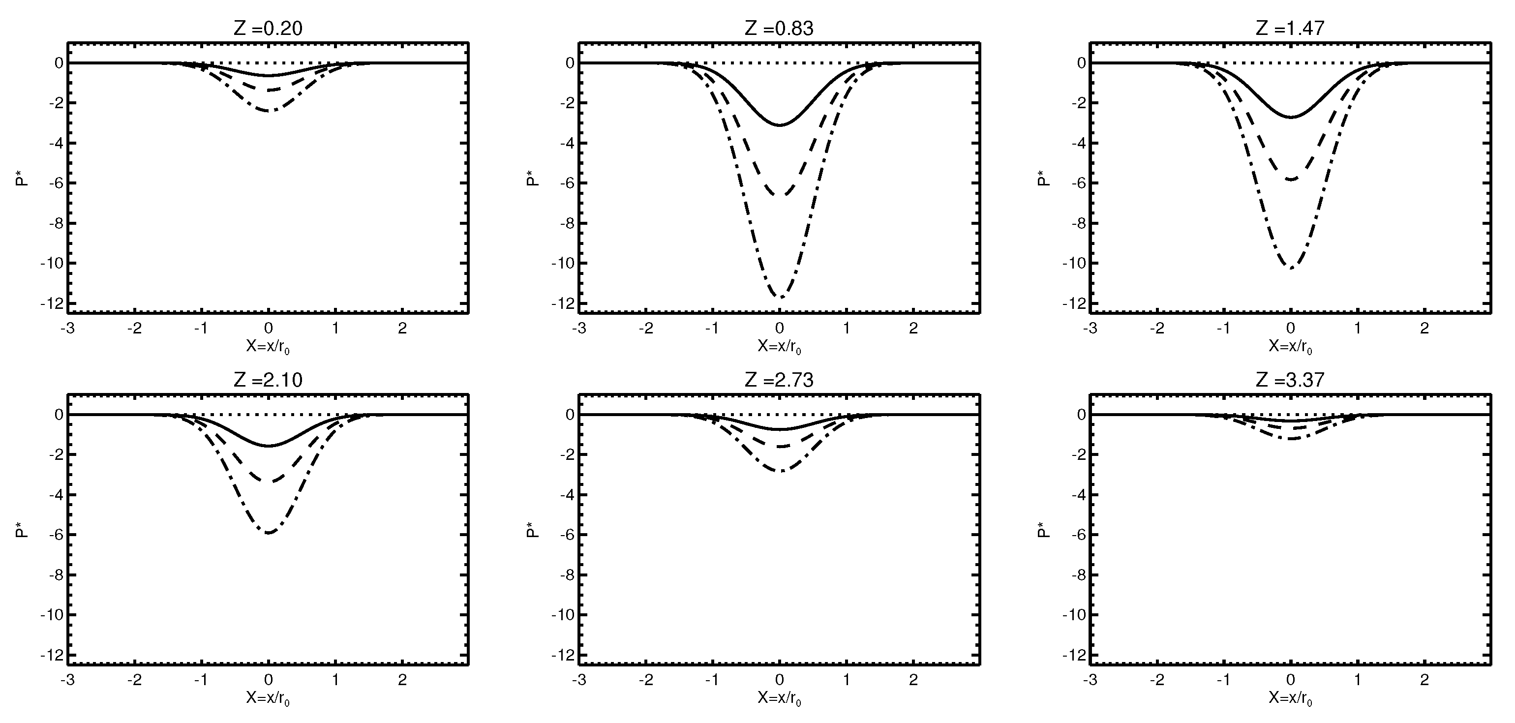
In the calculations of the particle trajectories it was assumed that at the initial radial position of the particles was . Figure 2 shows the radial distribution of dimensionless pressure at different heights for . The deep well of the lowered (negative) pressure in the central region of the vortex is due to the significant poloidal velocity components. The fluid in the region with negative pressure is sucked into the centre of the vortex.
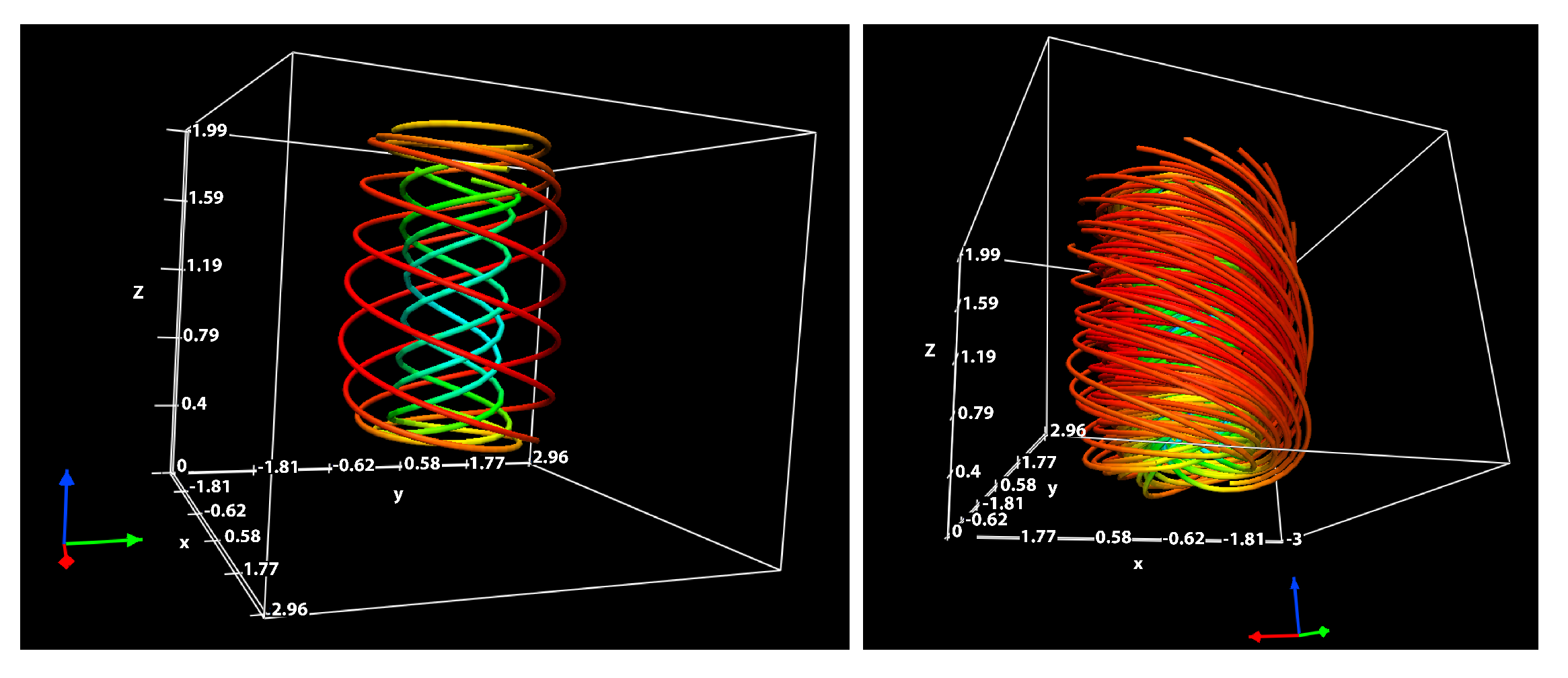
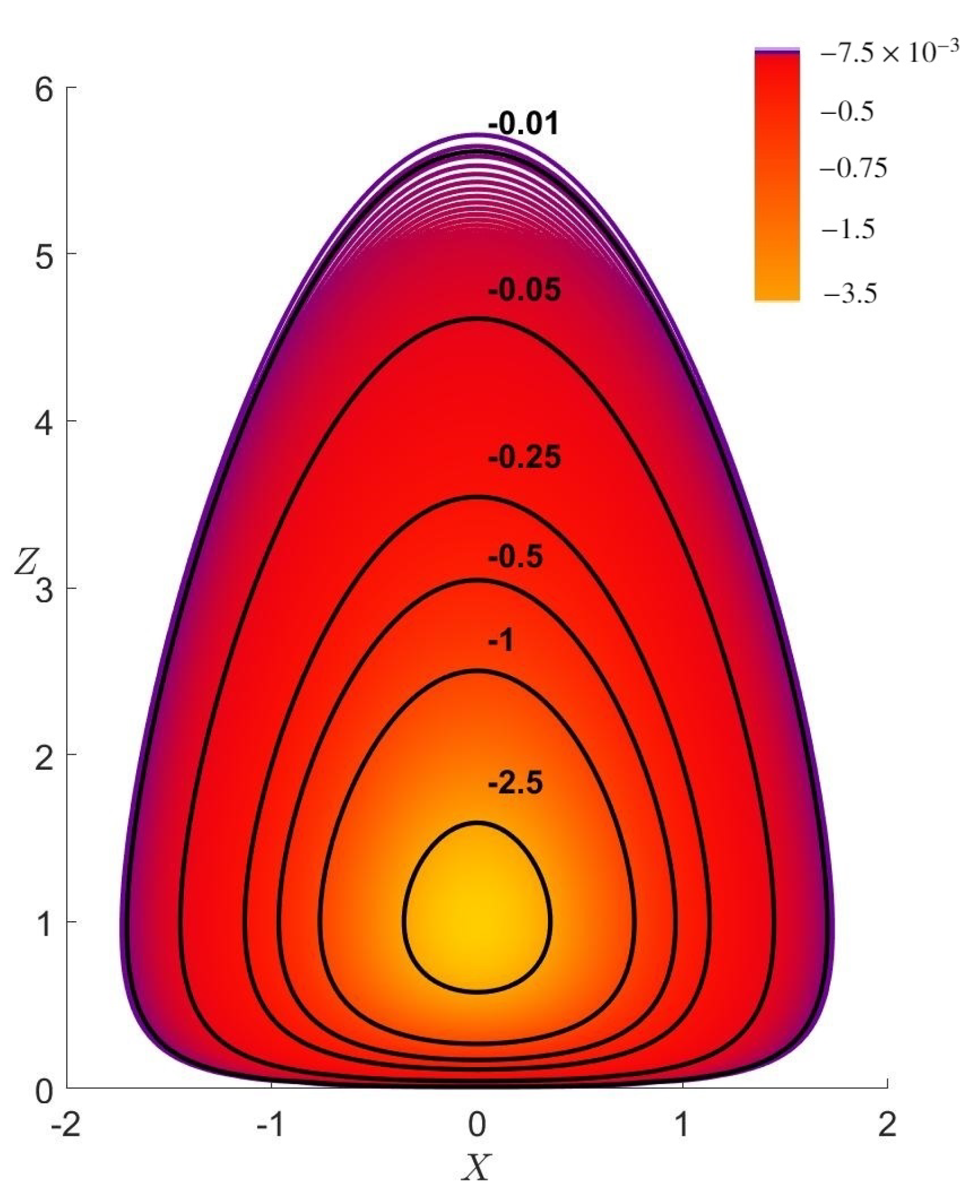
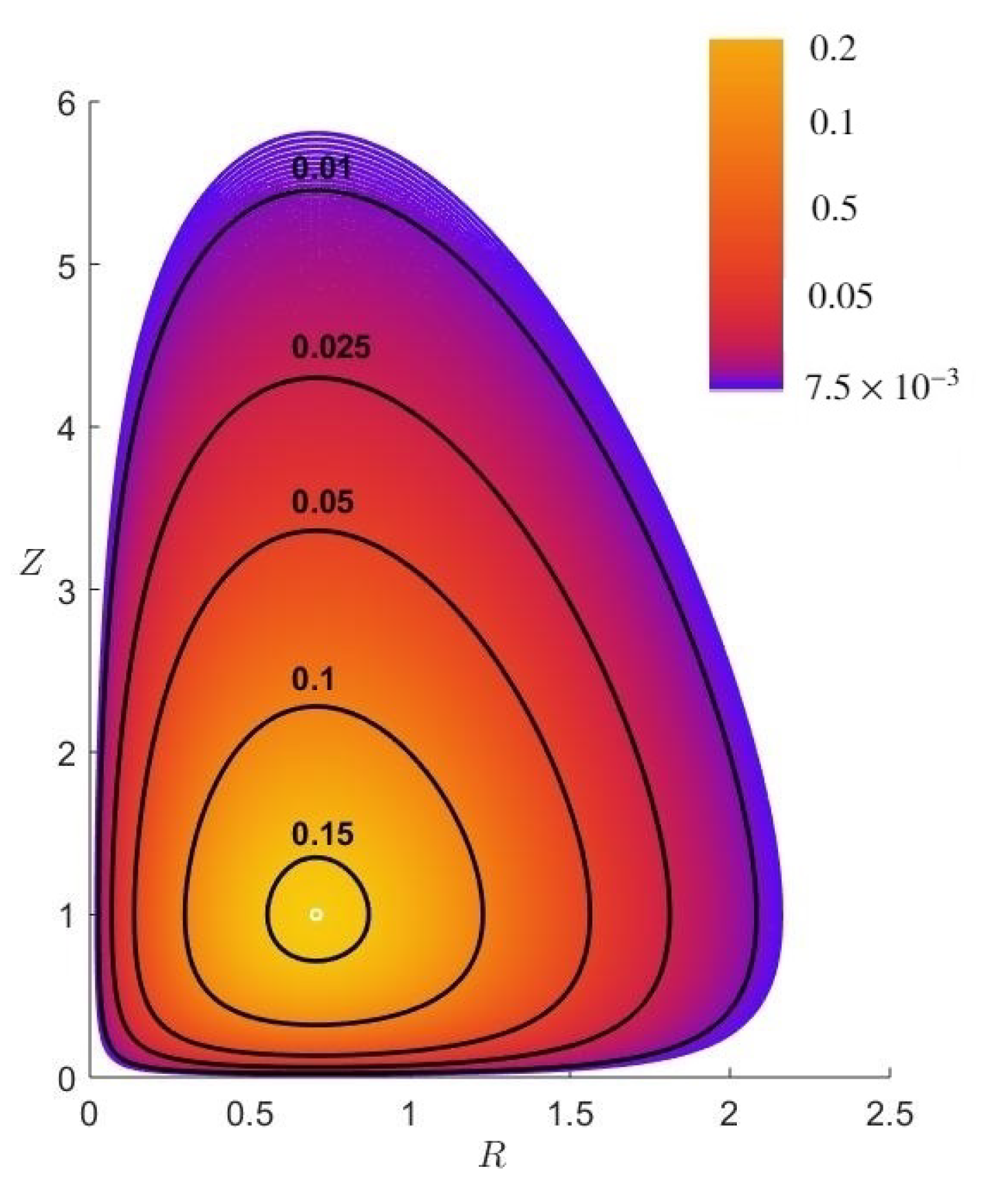
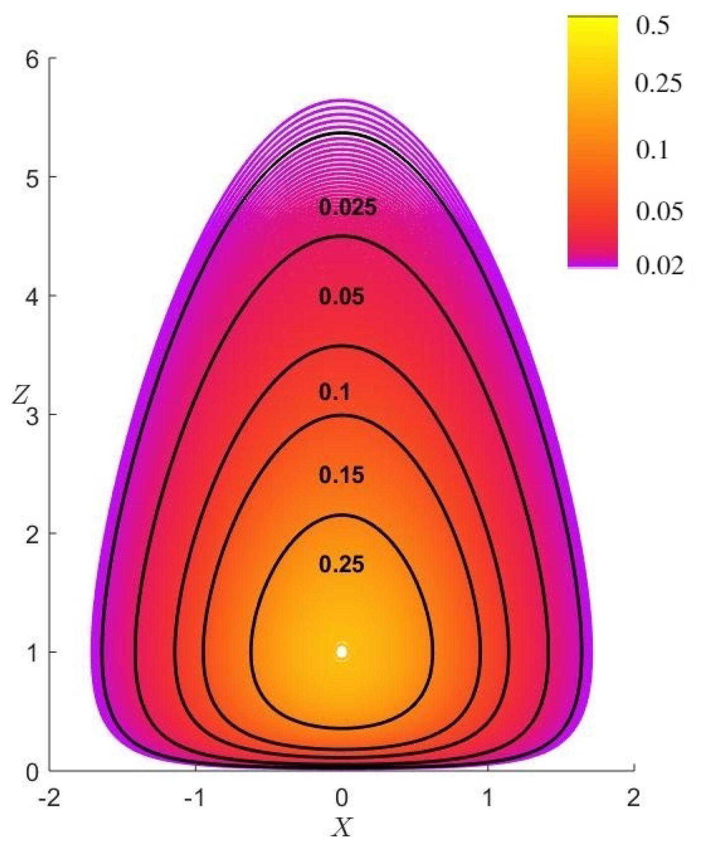
The illustration of the vortex model plotted for the the typical velocity ratio is shown in Figure 1, using VAPOR [57,58,59]. The normalised pressure for the values equal to 9.34, 14.0 and 18.7 are shown in Figure 2. Note that for other finite values of velocity ratios, these plots do not change qualitatively. Figure 3 shows radius–height plot of isobars. Figure 4 and Figure 5 illustrate the radius–height contour plots of dimensionless magnitude of the toroidal velocity, and stream function (angular momentum M surfaces) .
4. Conclusions
In this paper, the new axially-symmetric model of a steady state vortex localised in the radial and vertical directions vortices with incompressible and inviscid flow which is a solution to the Euler equations has been proposed. In the framework of the model, the vortex is exponentially localised, not only in the radial direction, but also in height. Unlike previous theoretical models, the vortex velocity, vorticity and pressure are characterised not only by a characteristic vortex radius , but also by a characteristic vortex height L.
According to observations [2,6] and numerical simulations [5,60], the behaviour of the toroidal velocity of vortices is similar to that in a stationary Rankine or Burgers vortices. However, for the description of poloidal motion in vortices, the models Burgers and Sullivan have a number of essential shortcomings that limit their applicability to concentrated vortices. In the Burgers and Sullivan models, the vertical velocity and pressure increase without bound with increasing altitude. The vertical velocity in the Burgers model is only a linear function of z, which means that the vertical velocity is not confined to any region, but is the same everywhere, i.e., it is not a concentrated vortex. The new low-parametrical model presented here, as well as having characteristic radial and vertical scales, also has characteristic poloidal and toroidal speeds. Furthermore, the pressure can be compared with observation and experiment, not only in the inner part of the vortex at , but also in the outer region at , and at heights comparable to the height of the vortex L. In this new model, when the vertical and radial mass flows are equal to zero, and , the condition of mass conservation is not required in contrast to Burgers and Sullivan models where there is an non-physical assumption about the source of mass. Recently, the new similarity criteria for the terrestrial and Martian convective structures were introduced in [61]. These criteria are fully applicable to the model developed in the present paper and can be used for obtaining the relationship between characteristic values of poloidal velocities and the spatial scales of vortex structures in the atmospheres of the Earth and Mars.
The vortex model developed here, as with the Burgers and Sullivan models, only satisfies inviscid boundary conditions and so falls far short of an adequate vortex description at a boundary. In fact, at a rigid boundary, the balanced centrifugal pressure field of the vortex core is disrupted in a thin terminating boundary layer in which a large radial inflow is driven by the unbalanced pressure field. These models are strictly only applicable above the frictional boundary layer, where the flow evolves approximately via balance dynamics effects [54,62]. It has been shown that the proposed new analytical model of concentrated vortices is in good agreement with field observations of typical dust vortices in the Earth’s atmosphere. This model can be also expanded on the magnetised plasma. This modification may be useful for interpretation of vortex behaviour in the solar atmosphere, but this is subject of future studies.
Author Contributions
Conceptualisation, O.O., V.F. and O.P.; methodology, O.O.; software, V.F., O.O. and S.J.S.; validation, O.O., V.F., O.P., W.H. and G.V.; formal analysis, V.F., O.O., O.P., W.H. and G.V.; investigation, O.O., V.F., O.P., W.H. and G.V.; resources, V.F.; writing—original draft preparation, O.O., V.F. and O.P.; writing—review and editing, O.O., V.F., S.J.S., O.P., W.H. and G.V.; visualisation, V.F. and S.J.S.; project administration, O.O. Formal analysis, W.H., O.P., N.A., S.J.S. and G.V.; Methodology, O.O.; Project administration, V.F.; Visualization, S.J.S. All authors have read and agreed to the published version of the manuscript.
Funding
We have provided this info in the acknowledgments.
Data Availability Statement
This is theoretical work, therefore there is no data associated with this research.
Acknowledgments
O.O. is thankful to the Program of Prezidium of the Russian Academy of Sciences No. 19-270 the state task of IPE RAS and the Russian Foundation for Basic research 18-29-21021 for the partial financial support. V.F. and G.V. give thanks to The Royal Society, International Exchanges Scheme, collaboration with Chile (IE170301) and Brazil (IES/R1/191114). V.F. and G.V. are grateful to the Science and Technology Facilities Council (STFC) grant ST/M000826/1 for support provided. This research is also partially funded by the European Unions Horizon 2020 research and innovation program under grant agreement No. 824135 (SOLARNET). W.H. thanks for partial support of the US Department of Energy under grant DE-FG02-04ER54742 and the Space and Geophysics Laboratory at The University of Texas at Austin. S.J.S. would like to thank the STFC studentship. This work also greatly benefited from the discussions at the ISSI workshops “Towards Dynamic Solar Atmospheric Magneto-Seismology with New Generation Instrumentation” and “The nature and physics of vortex flows in solar plasmas”. Finally, the authors are grateful to R. K. Smith whose insightful remarks helped us to improve the manuscript.
Conflicts of Interest
The authors declare no conflict of interest.
References
- Maxworthy, T. A Vorticity Source for Large-Scale Dust Devils and Other Comments on Naturally Occurring Columnar Vortices. J. Atmos. Sci. 1973, 30, 1717–1722. [Google Scholar] [CrossRef] [Green Version]
- Mullen, J.B.; Maxworthy, T. A laboratory model of dust devil vortices. Dyn. Atmos. Ocean. 1977, 1, 181–214. [Google Scholar] [CrossRef]
- Trapp, R.J.; Fiedler, B.H. Tornado-like Vortexgenesis in a Simplified Numerical Model. J. Atmos. Sci. 1995, 52, 3757–3778. [Google Scholar] [CrossRef] [Green Version]
- Kanak, K.M.; Lilly, D.K.; Snow, J.T. The formation of vertical Vortices in the convective boundary layer. Q. J. R. Meteorol. Soc. 2000, 126, 2789–2810. [Google Scholar] [CrossRef]
- Kanak, K.M. Numerical simulation of dust devil-scale vortices. Q. J. R. Meteorol. Soc. 2005, 131, 1271–1292. [Google Scholar] [CrossRef]
- Balme, M.; Greeley, R. Dust devils on Earth and Mars. Rev. Geophys. 2006, 44, RG3003. [Google Scholar] [CrossRef]
- Gu, Z.; Qiu, J.; Zhao, Y.; Li, Y. Simulation of terrestrial dust devil patterns. Adv. Atmos. Sci. 2008, 25, 31–42. [Google Scholar] [CrossRef]
- Zhao, Y.Z.; Gu, Z.L.; Yu, Y.Z.; Ge, Y.; Li, Y.; Feng, X. Mechanism and large eddy simulation of dust devils. Atmos. Ocean 2010, 61–84. [Google Scholar] [CrossRef] [Green Version]
- Raasch, S.; Franke, T. Structure and formation of dust devil-like vortices in the atmospheric boundary layer: A high-resolution numerical study. J. Geophys. Res. Atmos. 2011, 116, D16120. [Google Scholar] [CrossRef]
- Davies-Jones, R. A review of supercell and tornado dynamics. Atmos. Res. 2015, 158, 274–291. [Google Scholar] [CrossRef]
- Horton, W.; Miura, H.; Onishchenko, O.; Couedel, L.; Arnas, C.; Escarguel, A.; Benkadda, S.; Fedun, V. Dust devil dynamics. J. Geophys. Res. Atmos. 2016, 121, 7197–7214. [Google Scholar] [CrossRef] [Green Version]
- Neves, T.; Fisch, G.; Raasch, S. Local Convection and Turbulence in the Amazonia Using Large Eddy Simulation Model. Atmosphere 2018, 9, 399. [Google Scholar] [CrossRef] [Green Version]
- Farrell, W.M.; Delory, G.T.; Cummer, S.A.; Marshall, J.R. A simple electrodynamic model of a dust devil. Geophys. Res. Lett. 2003, 30, 2050. [Google Scholar] [CrossRef] [Green Version]
- Farrell, W.M.; Smith, P.H.; Delory, G.T.; Hillard, G.B.; Marshall, J.R.; Catling, D.; Hecht, M.; Tratt, D.M.; Renno, N.; Desch, M.D.; et al. Electric and magnetic signatures of dust devils from the 2000–2001 MATADOR desert tests. J. Geophys. Res. Planets 2004, 109, E03004. [Google Scholar] [CrossRef]
- Farrell, W.M.; Renno, N.; Delory, G.T.; Cummer, S.A.; Marshall, J.R. Integration of electrostatic and fluid dynamics within a dust devil. J. Geophys. Res. Planets 2006, 111, E01006. [Google Scholar] [CrossRef] [Green Version]
- Melnik, O.; Parrot, M. Electrostatic discharge in Martian dust storms. J. Geophys. Res. 1998, 103, 29107–29118. [Google Scholar] [CrossRef]
- Zhou, Y.H.; Guo, X.; Zheng, X.J. Experimental measurement of wind-sand flux and sand transport for naturally mixed sands. Phys. Rev. E 2002, 66, 021305. [Google Scholar] [CrossRef] [PubMed]
- Zheng, X.J.; Huang, N.; Zhou, Y.H. Laboratory measurement of electrification of wind-blown sands and simulation of its effect on sand saltation movement. J. Geophys. Res. Atmos. 2003, 108, 4322. [Google Scholar] [CrossRef]
- Xie, L.; Ling, Y.; Zheng, X. Laboratory measurement of saltating sand particles’ angular velocities and simulation of its effect on saltation trajectory. J. Geophys. Res. Atmos. 2007, 112, D12116. [Google Scholar] [CrossRef]
- Harrison, R.G.; Barth, E.; Esposito, F.; Merrison, J.; Montmessin, F.; Aplin, K.L.; Borlina, C.; Berthelier, J.J.; Déprez, G.; Farrell, W.M.; et al. Applications of Electrified Dust and Dust Devil Electrodynamics to Martian Atmospheric Electricity. Space Sci. Rev. 2016, 203, 299–345. [Google Scholar] [CrossRef] [Green Version]
- Izvekova, Y.N.; Popel, S.I. Charged Dust Motion in Dust Devils on Earth and Mars. Contrib. Plasma Phys. 2016, 56, 263–269. [Google Scholar] [CrossRef]
- Izvekova, Y.N.; Popel, S.I. Plasma Effects in Dust Devils near the Martian Surface. Plasma Phys. Rep. 2017, 43, 1172–1178. [Google Scholar] [CrossRef]
- Izvekova, Y.N.; Popel, S.I.; Izvekov, O.Y. On the Possibility of Excitation of Oscillations in a Schumann Resonator on Mars. Plasma Phys. Rep. 2020, 46, 65–70. [Google Scholar] [CrossRef]
- Izvekova, Y.N.; Reznichenko, Y.S.; Popel, S.I. On the Possibility of Dust Acoustic Perturbations in Martian Ionosphere. Plasma Phys. Rep. 2020, 46, 1205–1209. [Google Scholar] [CrossRef]
- Stenflo, L. Nonlinear equations for acoustic gravity waves. Phys. Lett. A 1996, 222, 378–380. [Google Scholar] [CrossRef]
- Shukla, P.K.; Stenflo, L. Acoustic gravity tornadoes in the atmosphere. Phys. Scr. 2012, 86, 065403. [Google Scholar] [CrossRef]
- Sinclair, P.C. General Characteristics of Dust Devils. J. Appl. Meteorol. 1969, 8, 32–45. [Google Scholar] [CrossRef] [Green Version]
- Onishchenko, O.; Pokhotelov, O.; Fedun, V. Convective cells of internal gravity waves in the earth’s atmosphere with finite temperature gradient. Ann. Geophys. 2013, 31, 459–462. [Google Scholar] [CrossRef] [Green Version]
- Onishchenko, O.; Pokhotelov, O.; Horton, W.; Fedun, V. Dust devil vortex generation from convective cells. Ann. Geophys. 2015, 33, 1343–1347. [Google Scholar] [CrossRef] [Green Version]
- Onishchenko, O.G.; Horton, W.; Pokhotelov, O.A.; Fedun, V. “Explosively growing” vortices of unstably stratified atmosphere. J. Geophys. Res. Atmos. 2016, 121, 11. [Google Scholar] [CrossRef]
- Rafkin, S.; Jemmett-Smith, B.; Fenton, L.; Lorenz, R.; Takemi, T.; Ito, J.; Tyler, D. Dust Devil Formation. Space Sci. Rev. 2016, 203, 183–207. [Google Scholar] [CrossRef]
- Rennó, N.O.; Burkett, M.L.; Larkin, M.P. A Simple Thermodynamical Theory for Dust Devils. J. Atmos. Sci. 1998, 55, 3244–3252. [Google Scholar] [CrossRef]
- Smith, R.K.; Leslie, L.M. Thermally driven vortices: A numerical study with application to dust-devil dynamics. Q. J. R. Meteorol. Soc. 1976, 102, 791–804. [Google Scholar] [CrossRef]
- Hicks, W.M. Researches in Vortex Motion. Part III: On Spiral or Gyrostatic Vortex Aggregates. Philos. Trans. R. Soc. Lond. Ser. A 1899, 192, 33–99. [Google Scholar] [CrossRef] [Green Version]
- Moffatt, H.K. The degree of knottedness of tangled vortex lines. J. Fluid Mech. 1969, 35, 117–129. [Google Scholar] [CrossRef]
- Wu, J.Z.; Ma, H.Y.; Zhou, M.D. Vorticity and Vortex Dynamics. 2006. Available online: https://0-www-springer-com.brum.beds.ac.uk/gp/book/9783540290278 (accessed on 5 January 2021).
- Onishchenko, O.G.; Pokhotelov, O.A.; Astafieva, N.M. A Novel Model of Quasi-Stationary Vortices in the Earth’s Atmosphere. Izv. Atmos. Ocean. Phys. 2018, 54, 906–910. [Google Scholar] [CrossRef]
- Onishchenko, O.; Pokhotelov, O.; Horton, W.; Smolyakov, A.; Kaladze, T.; Fedun, V. Rolls of the internal gravity waves in the Earth’s atmosphere. Ann. Geophys. 2014, 32, 181–186. [Google Scholar] [CrossRef] [Green Version]
- Onishchenko, O.G.; Fedun, V.; Horton, W.; Pokhotelov, O.; Verth, G. Dust devils: Structural features, dynamics and climate impact. Climate 2019, 7, 12. [Google Scholar] [CrossRef] [Green Version]
- Onishchenko, O.G.; Pokhotelov, O.; Astafieva, N.M.; Horton, W.; Fedun, V. Structure and dynamics of concentrated mesoscale vortices in the atmospheres of planets. Phys. Usp. 2020. [Google Scholar] [CrossRef]
- Rankine, W.J.M. A Manual of Applied Mechanics; Charles Griffin and Company Limited: London, UK, 1901. [Google Scholar]
- Battan, L.J. Energy of a Dust Devil. J. Atmos. Sci. 1958, 15, 235–236. [Google Scholar] [CrossRef] [Green Version]
- Sinclair, P.C. on the rotation of dust devils. Bull. Am. Meteorol. Soc. 1965, 46, 388–391. [Google Scholar] [CrossRef]
- Sinclair, P.C. The Lower Structure of Dust Devils. J. Atmos. Sci. 1973, 30, 1599–1619. [Google Scholar] [CrossRef]
- Williams, N.R. Development of Dust Whirls and Similar Small-Scale Vortices. Bull. Am. Meteorol. Soc. 1948, 29, 106–117. [Google Scholar] [CrossRef] [Green Version]
- Bluestein, H.B.; Weiss, C.C.; Pazmany, A.L. Doppler Radar Observations of Dust Devils in Texas. Mon. Weather Rev. 2004, 132, 209. [Google Scholar] [CrossRef]
- Toigo, A.D.; Richardson, M.I.; Ewald, S.P.; Gierasch, P.J. Numerical simulation of Martian dust devils. J. Geophys. Res. Planets 2003, 108, 5047. [Google Scholar] [CrossRef] [Green Version]
- Kurgansky, M.V. A simple model of dry convective helical vortices (with applications to the atmospheric dust devil). Dyn. Atmos. Ocean. 2005, 40, 151–162. [Google Scholar] [CrossRef]
- Kurgansky, M.V.; Lorenz, R.D.; Renno, N.O.; Takemi, T.; Gu, Z.; Wei, W. Dust Devil Steady-State Structure from a Fluid Dynamics Perspective. Space Sci. Rev. 2016, 203, 209–244. [Google Scholar] [CrossRef]
- Burgers, J.M. A mathematical model illustrating the theory of turbulence. Adv. Appl. Mech. 1948, 1, 171–199. [Google Scholar] [CrossRef]
- Rott, N. On the viscous core of a line vortex. Z. Angew. Math. Und Phys. 1958, 9, 543–553. [Google Scholar] [CrossRef]
- Sullivan, R.D. A Two-Cell Vortex Solution of the Navier-Stokes Equations. J. Aerosp. Sci. 1959, 26, 767–768. [Google Scholar] [CrossRef]
- Michaels, I.T.; Rafkin Scot, C.R. Large-eddy simulation of atmospheric convection on Mars. Q. J. R. Meteorol. Soc. 2004, 130, 1251–1274. [Google Scholar] [CrossRef] [Green Version]
- Morton, B.R. The strength of vortex and swirling core flows. J. Fluid Mech. 1969, 38, 315–333. [Google Scholar] [CrossRef]
- Velikhov, E.P. Stability of an ideally conducting liquid flowing between cylinders rotating in a magnetic field. JETP 1959, 36, 1398–1404. [Google Scholar]
- Chandrasekhar, S. Hydrodynamic and Hydromagnetic Stability; Courier Corporation: Chelmsford, MA, USA, 1961. [Google Scholar]
- Clyne, J.; Mininni, P.; Norton, A.; Rast, M. Interactive desktop analysis of high resolution simulations: Application to turbulent plume dynamics and current sheet formation. New J. Phys. 2007, 9, 301. [Google Scholar] [CrossRef] [Green Version]
- Clyne, J.; Rast, M. Visualization and Data Analysis 2005. In A Prototype Discovery Environment for Analyzing and Visualizing Terascale Turbulent Fluid Flow Simulations; Erbacher, R.F., Roberts, J.C., Gröhn, M.T., Börner, K., Eds.; International Society for Optics and Photonics: Bellingham, WA, USA, 2005; Volume 5669, pp. 284–294. [Google Scholar] [CrossRef]
- Li, S.; Jaroszynski, S.; Pearse, S.; Orf, L.; Clyne, J. VAPOR: A Visualization Package Tailored to Analyze Simulation Data in Earth System Science. Atmosphere 2019, 10, 488. [Google Scholar] [CrossRef] [Green Version]
- Spiga, A.; Barth, E.; Gu, Z.; Hoffmann, F.; Ito, J.; Jemmett-Smith, B.; Klose, M.; Nishizawa, S.; Raasch, S.; Rafkin, S.; et al. Large-Eddy Simulations of Dust Devils and Convective Vortices. Space Sci. Rev. 2016, 203, 245–275. [Google Scholar] [CrossRef] [Green Version]
- Izvekova, Y.N.; Popel’, S.I.; Izvekov, O.Y. On the Question of Calculating the Parameters of Vortices in the Near-Surface Atmosphere of Mars. Sol. Syst. Res. 2020, 53, 423–430. [Google Scholar] [CrossRef]
- Smith, R.K.; Montgomery, M.T.; Persing, J. On steady-state tropical cyclones. Q. J. R. Meteorol. Soc. 2014, 140, 2638–2649. [Google Scholar] [CrossRef]
Figure 1.
The normalised three-dimensional stream lines of the vortex velocity field. On the left panel only four stream lines are shown. The light blue and green colours of the stream lines correspond to the internal structure of the vortex. The red and amber colours correspond to the external part of the vortex. On the right panel more than forty velocity stream lines are shown. The red, green and blue orthogonal vectors colours indicate the x, y and z axis, correspondingly. The visualisation was computed for and .

Figure 2.
The behaviour of the normalised pressure across the vortex at different heights for the values of equal to 9.34, 14.0 and 18.7 (solid, dash and dash-dot plots, correspondingly).
Figure 2.
The behaviour of the normalised pressure across the vortex at different heights for the values of equal to 9.34, 14.0 and 18.7 (solid, dash and dash-dot plots, correspondingly).

Figure 3.
The radius–height plot of dimensionless isobars for . Axis labels given by and , where .

Figure 4.
The radius–height contour plots of dimensionless toroidal velocity, . Axis labels given by and .
Figure 4.
The radius–height contour plots of dimensionless toroidal velocity, . Axis labels given by and .

Figure 5.
The dimensionless stream functions (or angular momentum surfaces) . Axis labels given by and , where .
Figure 5.
The dimensionless stream functions (or angular momentum surfaces) . Axis labels given by and , where .

Publisher’s Note: MDPI stays neutral with regard to jurisdictional claims in published maps and institutional affiliations. |
© 2021 by the authors. Licensee MDPI, Basel, Switzerland. This article is an open access article distributed under the terms and conditions of the Creative Commons Attribution (CC BY) license (http://creativecommons.org/licenses/by/4.0/).
Share and Cite
MDPI and ACS Style
Onishchenko, O.; Fedun, V.; Horton, W.; Pokhotelov, O.; Astafieva, N.; Skirvin, S.J.; Verth, G. The Stationary Concentrated Vortex Model. Climate 2021, 9, 39. https://0-doi-org.brum.beds.ac.uk/10.3390/cli9030039
AMA Style
Onishchenko O, Fedun V, Horton W, Pokhotelov O, Astafieva N, Skirvin SJ, Verth G. The Stationary Concentrated Vortex Model. Climate. 2021; 9(3):39. https://0-doi-org.brum.beds.ac.uk/10.3390/cli9030039
Chicago/Turabian StyleOnishchenko, Oleg, Viktor Fedun, Wendell Horton, Oleg Pokhotelov, Natalia Astafieva, Samuel J. Skirvin, and Gary Verth. 2021. "The Stationary Concentrated Vortex Model" Climate 9, no. 3: 39. https://0-doi-org.brum.beds.ac.uk/10.3390/cli9030039
Note that from the first issue of 2016, this journal uses article numbers instead of page numbers. See further details here.