
Evolution of the Arabian Sea Upwelling from the Last Millennium to the Future as Simulated by Earth System Models


Institute of Coastal Systems Analysis and Modeling, Helmholtz-Zentrum Hereon, Max-Planck-Str.1, 21502 Geesthacht, Germany
*
Author to whom correspondence should be addressed.
Climate 2021, 9(5), 72; https://0-doi-org.brum.beds.ac.uk/10.3390/cli9050072
Submission received: 18 March 2021
/
Revised: 26 April 2021
/
Accepted: 27 April 2021
/
Published: 29 April 2021
Abstract
:Arabian Sea upwelling in the past has been generally studied based on the sediment records. We apply two earth system models and analyze the simulated water vertical velocity to investigate coastal upwelling in the western Arabian Sea over the last millennium. In addition, two models with slightly different configurations are also employed to study the upwelling in the 21st century under the strongest and the weakest greenhouse gas emission scenarios. With a negative long-term trend caused by the orbital forcing of the models, the upwelling over the last millennium is found to be closely correlated with the sea surface temperature, the Indian summer Monsoon and the sediment records. The future upwelling under the Representative Concentration Pathway (RCP) 8.5 scenario reveals a negative trend, in contrast with the positive trend displayed by the upwelling favorable along-shore winds. Therefore, it is likely that other factors, like water stratification in the upper ocean layers caused by the stronger surface warming, overrides the effect from the upwelling favorable wind. No significant trend is found for the upwelling under the RCP2.6 scenario, which is likely due to a compensation between the opposing effects of the increase in upwelling favorable winds and the water stratification.
1. Introduction
Upwelling lifts the cold nutrient-rich water from deeper ocean layers to the surface, which cools the surface water and provides the biologically active layers with nutrients. It has a great impact on human activities. For instance, about 20% of the total marine fish catches originate from upwelling regions that cover only 2% of the entire ocean area [1]. Upwelling also affects the climate by cooling the sea surface temperature (SST) and by influencing the air–sea interactions associated with the variation of SST [2]. It has been suggested that as one of the climatic effects, under the global warming scenario, coastal upwelling at global scale would be intensified as the upwelling favorable wind-stress would be strengthened due to the enhanced air–sea temperature gradient [3]. Numerous studies have provided insights into the upwelling variations over the last few decades. Most of these studies focus on the four major eastern boundary upwelling systems (EBUSs), namely, the California [4], Canary [5], Humboldt [6] and Benguela [7] upwelling systems. In support of the upwelling intensification hypothesis by Bakun [3], Narayan et al. [8] found positive trends over the late 20th century in all these four coastal upwelling regions and Sydeman et al. [9] also reported upwelling intensification in the major EBUSs after synthesizing the results from previous studies.
In addition to the major EBUSs, the Arabian Sea is one of the most productive regions in the world [10]. The coastal upwelling in the western Arabian Sea is mainly driven by the southwest (SW) wind-stress, which is induced by the Indian summer Monsoon (ISM) [11]. Since the link between the ISM and the upwelling is very pronounced, many studies have used the ISM as an indicator of the upwelling, and vice versa [12,13,14]. However, direct observations of upwelling in terms of water mass vertical velocity over a long time period are rare, thus, alternative upwelling proxies such as SST, surface wind-stress and sediment records have been generally applied. An alternative tool to analyze upwelling variability is provided by model simulations.
The knowledge of upwelling evolution in the past is crucial to understand and model the upwelling variations at present and to predict them in the future. A widespread approach to study upwelling in the past is through sediment records where the abundance of G. bulloides is stored. G. bulloides belongs to the phylum foraminifera and is very sensitive to upwelling variations so it is generally used as an upwelling proxy. Over the last millennium, the Arabian Sea upwelling is reported to exhibit a slight decrease until approximately 1600 and an abrupt increase afterwards [15,16,17]. As for the future, whereas a study focused on the Arabian Sea upwelling is not yet available, Wang et al. [18] used the Coupled Model Intercomparison Project Phase 5 (CMIP5) [19] model outputs to conduct an analysis on the 21st century upwelling under the future scenario of Representative Concentration Pathway (RCP) 8.5. They indicated that the upwelling intensity and duration are both increased at high latitudes in most of the major EBUSs except California. The RCP8.5, along with the RCP6.0, RCP4.5 and RCP2.6 are labeled by the aimed radiative forcing in the year 2100, namely 8.5, 6.0, 4.5, and 2.6 W·m−2 [20]. The RCP scenarios imply several variables for the next centuries such as concentration of greenhouse gases, coverage of land use and chemically active gases. It is known that the external climate forcings are different over the last millennium and in the future. The responses to these forcings are also different among the major EBUSs [21]. Therefore, in the present study we analyze the impact of the external climate forcings on the Arabian Sea upwelling system and whether its response to the past can be linked with that to the future.
We investigate here the Arabian Sea upwelling variation over the last millennium by analyzing model simulations of water vertical velocity and by comparing the model results with the observational sediment records to determine the existence of the long-term trends. The evolution of future upwelling in the Arabian Sea is also investigated by using models with slightly different configurations from the last millennium simulations. We compare the future upwelling modeled under the RCP8.5 and RCP2.6 scenarios to gain the information on how the greenhouse gas emission level could affect the variation of upwelling.
2. Model and Data
Earth system models, in a way similarly to weather prediction models, include a numerical representation of the Earth’s atmosphere, ocean, land, sea-ice, and their physical and geochemical interactions. This numerical representation is to a large extent based on the known physical and chemical laws of momentum, energy and matter transfer, but also includes heuristic representations of small-scale processes (such as turbulence) that cannot be realistically resolved due to the still coarse spatial resolution of these models of about 100 km. The interested reader is referred to Edwards [22].
In this study, we selected four earth system models from the CMIP5 model pool, which have the highest horizontal resolution to study the Arabian Sea upwelling. The outputs from two of these models are used for the last millennium study and the other two, which are similar to the previous ones but with slightly different configurations, were applied for the future scenarios. For the analysis over the last millennium, we used the paleo configuration of the Earth System Model of Max-Planck Institute for Meteorology (MPI-ESM-P) [23] and the Last Millennium Ensemble (LME) project [24] of the Community Atmosphere Model Version 5 from CESM (CESM-CAM5) [25]. To estimate the upwelling variabilities in the future, we applied the low resolution configuration of the MPI-ESM (MPI-ESM-LR) and the Community Climate System Model (CCSM4), which is the predecessor of the CESM. Note that the CCSM4 uses a different version of atmosphere model (CAM4) than the CESM (CAM5).
The MPI-ESM-P and the MPI-ESM-LR share the same horizontal resolutions of about 2 degrees for the atmosphere (192 × 96) and about 1 degree for the ocean (256 × 220). Their vertical resolutions are the same as well with 47 levels for the atmosphere and 40 levels for the ocean. In spite of this, the MPI-ESM-P is available for the last millennium (850–1849) and the MPI-ESM-LR covers the future period (2006–2100) simulated under the greenhouse gas emission scenarios. The CESM-CAM5 and the CCSM4 also have identical horizontal resolutions for the ocean, which is about 1 degree on the longitude and 0.5 degrees on the latitude (320 × 384). For the atmosphere, the CESM-CAM5 has a horizontal resolution of 2.5 degrees on the longitude and 1.875 degrees on the latitude (144 × 96), which is four times coarser than the CCSM4 (288 × 192). On the vertical, they share the same resolutions with 60 levels in the ocean and 30 levels in the atmosphere. The CESM-CAM5 covers the last millennium period (850–1849) and the CCSM4 covers the 21st century (2005–2100). In the last millennium models, the external forcings are prescribed by a CMIP5 project defined standard protocol [26], which consists of solar irradiance variability [27], orbital forcing [28], volcanic activity [29,30], land-use changes [31] and greenhouse gases concentration [32,33,34]. For the future simulations, only the anthropogenic forcing is changed based on the RCP scenarios. The MPI-ESM-P and the MPI-ESM-LR each have an ensemble of three simulations while the CESM-CAM5 and the CCSM4 have ensembles of 13 simulations. Thus, we selected the first three simulations from each of them to compare with the MPI-ESM models. The differences between simulations within each ensemble provide an estimation of the amplitude of the effect of internal climate variability, whereas the signal shared by all simulations will approximate the response to the imposed external forcing [21].
We investigated several variables that are modeled by the simulations, including upwelling velocity, sea surface temperature (SST), surface wind-stress, zonal wind speed, and sea level pressure (SLP). The upwelling velocity is the “vertical velocity” in the CESM ensembles but has to be calculated from the “vertical water mass transport” for the MPI-ESM ensembles. Since coastal upwelling in the western Arabian Sea occurs from 200 m below the ocean surface [35], we averaged the upper 200 m of the data. We used the monthly data from the models and because the upwelling season starts in May and ends in September [36], only the summer months June, July and August (JJA) were selected. One exception is that for the SST we chose July, August and September (JAS) due to the lag in the response of SST to the upwelling [37]. In addition to the modeled data, we also applied the sediment records used by Anderson et al. [15] to compare with our results.
3. Results
3.1. Arabian Sea Upwelling in the Last Millennium
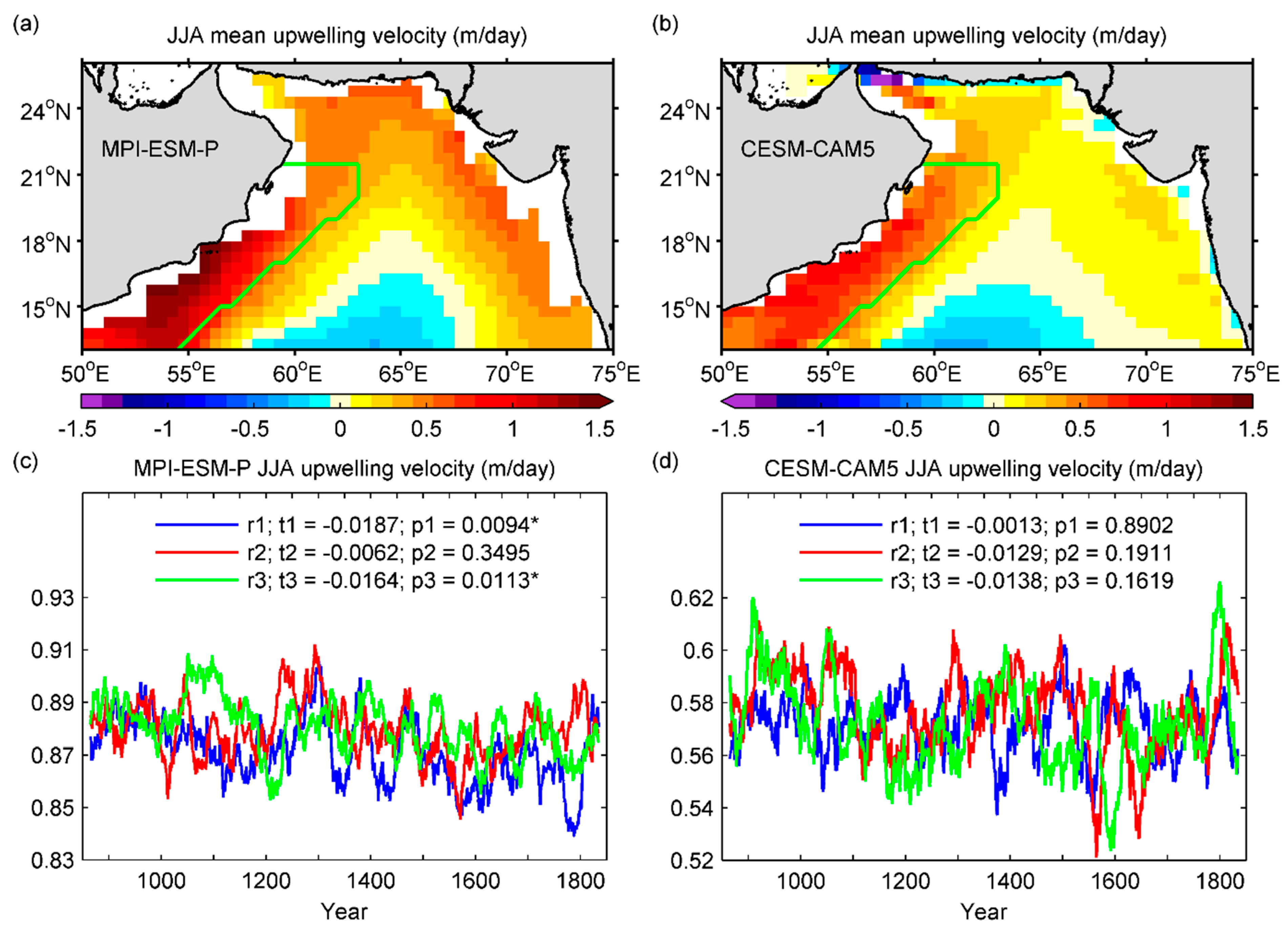
The mean summer upwelling velocities in the Arabian Sea modeled by MPI-ESM-P and CESM-CAM5 for the last millennium are presented in Figure 1. To avoid duplication, we only show the results of one simulation from each of these two simulation ensembles since the three simulations in each ensemble share very similar spatial patterns. The models present similar patterns of the summer upwelling in the Arabian Sea where strong upwelling occurs along the coast especially in the western Arabian Sea, induced by the southwest wind-stress (Figure 1a,b). Coastal upwelling in the western Arabian Sea is more intense in the MPI-ESM-P simulation, where the velocity can reach 1.5 m/day, than in CESM-CAM5 where the maximum velocity is around 1 m/day. The magnitude of these velocities is reasonable as it matches the estimated order of magnitude suggested from studies focused on present time period [37,38,39]. In addition, weak downwelling in the central Arabian Sea is found in both models. Downwelling here results from the convergence zone generated by the wind-stress curl [10,40]. Thus, the spatial distribution of the vertical velocity is consistent with the Ekman pumping effect [41].
We averaged the upwelling along the coast and calculate the upwelling velocity time series of this area (Figure 1c,d). This selected area spans about 5 degrees (500 km) from the coastline to the open ocean (shown within the green line in Figure 1a,b). Although the coastal upwelling in this region is reported to extend about 100 km from the coast towards offshore [37], such a narrow selection is not possible in our case due to the coarse resolutions of the models. In our selected study area, the upward vertical velocity actually presents upwelling induced by the combination of the SW wind-stress and the wind-stress curl. Therefore, when using the simulated upwelling velocity in the study area, the effects of Ekman transport and Ekman suction are not separated. This is also reasonable because the along-shore SW wind-stress is highly correlated with the off-shore wind-stress curl since they are both driven by the land–sea pressure gradient. In general, the time series show that on average, the mean upwelling velocity modeled by MPI-ESM-P is larger than the one simulated by CESM-CAM5 by around 0.3 m/day. The multidecadal variation is, however, larger in CESM-CAM5. All six simulations by the two models reveal negative trends of the upwelling velocity. A detailed interpretation of these trends and their significance level will be presented in Section 3.3.
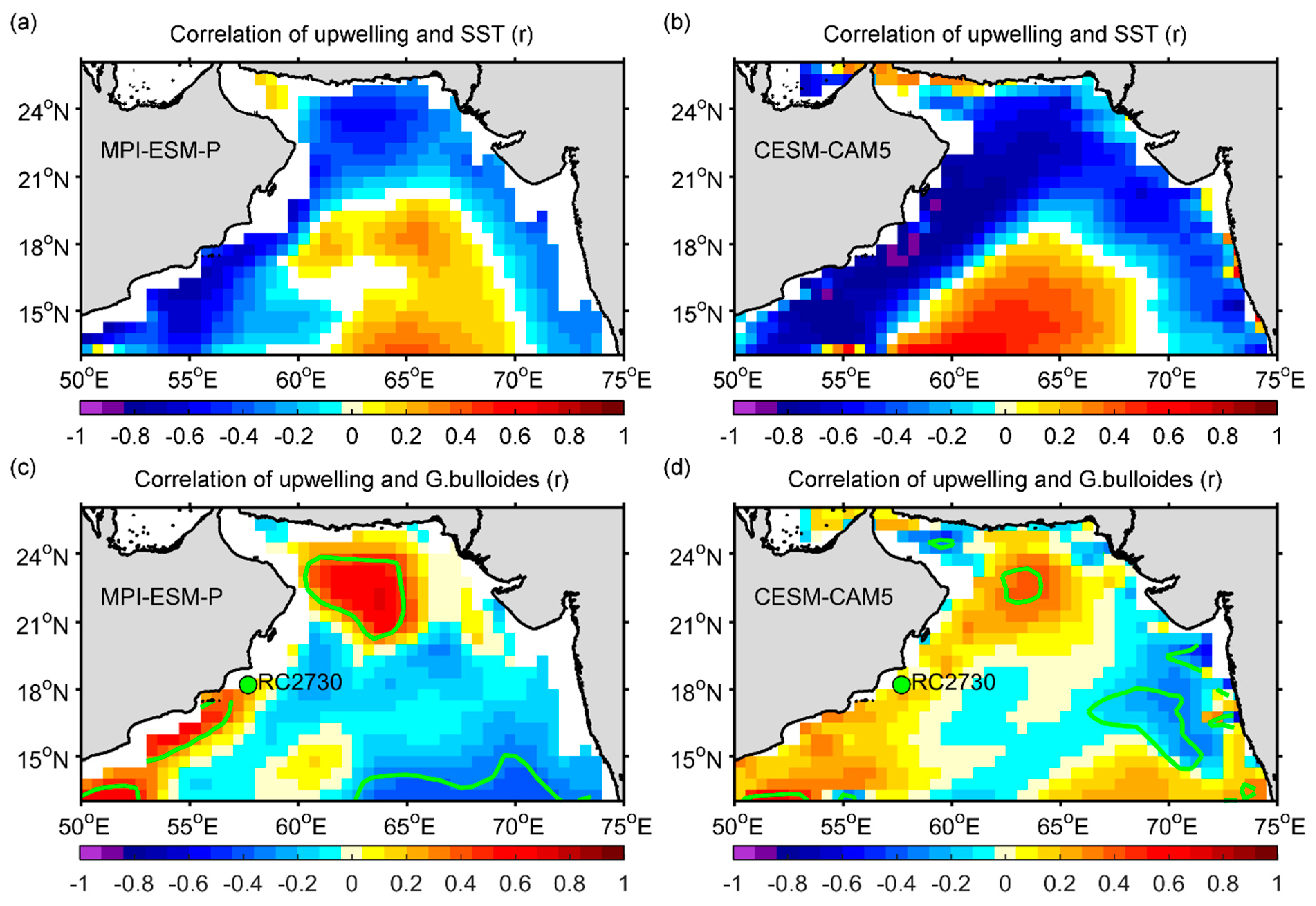
Since upwelling lifts the cold water from the deeper layers to the ocean surface during the upwelling season, the SST is often anticorrelated with upwelling in the upwelling region. This relationship is well captured in both of the models (Figure 2a,b). Strong negative correlations are shown along the coastal upwelling regions and even greater (r < −0.8) values are found at some locations in the western Arabian Sea in the CESM-CAM5 model. We also notice the positive correlation areas in the central Arabian Sea where weak downwelling is revealed as shown in Figure 1a,b. Downwelling is normally associated with convergence zones at the surface and weaker (stronger) downwelling is related to cooler (warmer) surface water in the same region. In terms of vertical velocity as it is in our case, downwelling is represented by the negative values of vertical velocities, thus, larger (smaller) velocities indicate weaker (stronger) downwelling. In principle, the SST should be negatively correlated with the vertical velocities in both upwelling and downwelling regions. However, Figure 2a,b shows positive correlations between SST and vertical velocity in the downwelling region of central Arabian Sea. This is likely due to the effect of horizontal advection [42,43], which transports the cold water mass raised by the coastal upwelling from the western to the central Arabian Sea. This cold water mass dominates the SST variability in the central Arabian Sea because the influence of the weak downwelling on the local SST is very small.
As a comparison with the sediment records, which is considered as the observational data, Figure 2c,d shows the correlations between Arabian Sea upwelling and the G. bulloides abundance retrieved from the sediment cores RC2730 and RC2735 [15]. This record has been interpreted as an indicator of upwelling in this region [44]. We only mark the location of RC2730 on the maps because these two cores are located very close to each other. The calculation of the correlation is performed on the 50-year averaged data during the overlapping years (1050–1849) of our modeled upwelling velocity and the G. bulloides abundance. To account for autocorrelation, we applied the nonparametric resampling method suggested by Ebisuzaki [45] to estimate the significance level of the correlations. These filtered series presumably reflect the variations in the external forcing, or at least the externally forced component of the variability should be large. Since the external forcing should be ideally the same in the observations and in the simulations, a positive correlation between both records should be expected. However, the records from only two cores located at very close positions might not represent the upwelling in a broader area. In spite of this, the maps present significant correlations along the coast all the way to the northern Arabian Sea, especially for the MPI-ESM-P model. Such correlations indicate that the models reasonably reproduce the variability of upwelling velocities at time scales that are presumably driven by the external climate forcing. The simulated records are thus comparable to the sediment records.
It has to be noted that the comparison between the modeled upwelling and the G. bulloides abundance does not aim to validate the model but to reveal the effect of external forcing. The correlations vary largely among the simulations as shown in Table 1 and are not significant everywhere in the study area (Figure 2), which raises uncertainty of the results. However, as mentioned before, the limitation of the G. bulloides abundance sample size and the sampling location exist. In spite of that, these results reflect the effects of external forcing on both the model outputs and the observation.
3.2. EOF Analysis of Upwelling
We performed an empirical orthogonal function (EOF) analysis [46] on the Arabian Sea upwelling to identify its main spatial variation patterns and the corresponding temporal evolutions. EOF analysis can identify the spatial patterns, which describe the data variance, by generating the EOF modes and their corresponding principal component (PC) time series, where each mode is ranked by its explained proportion of the total variance.
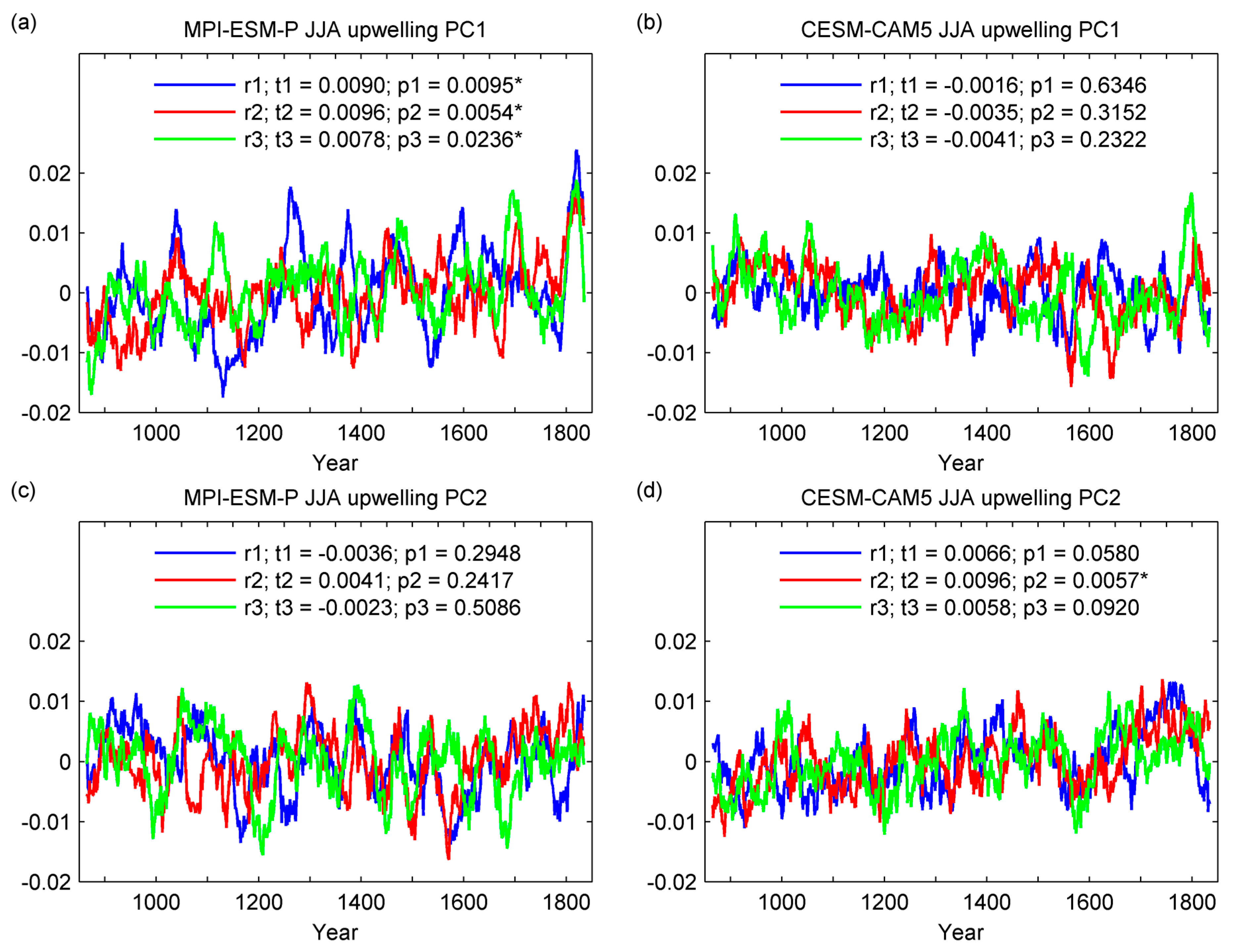
The leading two modes from the EOF analysis of the upwelling are given in Figure 3. The ranks of the first two modes are switched between MPI-ESM-P and CESM-CAM5. The first mode from CESM-CAM5 (Figure 3b) accounts for 41% of the total variance and reveals similar spatial patterns to the second mode of the MPI-ESM-P simulation (Figure 3c), which accounts for 24% of the total variance. We find that these EOF modes are related to the interannual variations as they capture the spatial patterns of the mean state of the upwelling (Figure 1a,b) where the different signs between coastal and central Arabian Seas show the contrast between these regions. Their PC time series (Figure 4b,c) also have a strong positive correlation with the time series averaged from the coastal upwelling in the western Arabian Sea (Figure 1c,d) for all the simulations, respectively (Table 1).
Thus, the intensity of the coastal upwelling in the western Arabian Sea is in phase with the intensity of the upwelling in the rest of the coastal areas and also with the intensity of the downwelling in the central Arabian Sea. This result is supported by the correlation between upwelling and the Indian Monsoon Index (IMI). We calculated the IMI from the model derived U850 wind data based on the definition of Wang and Fan [47]. The IMI is significantly correlated to our upwelling time series in all the simulations (Table 1).
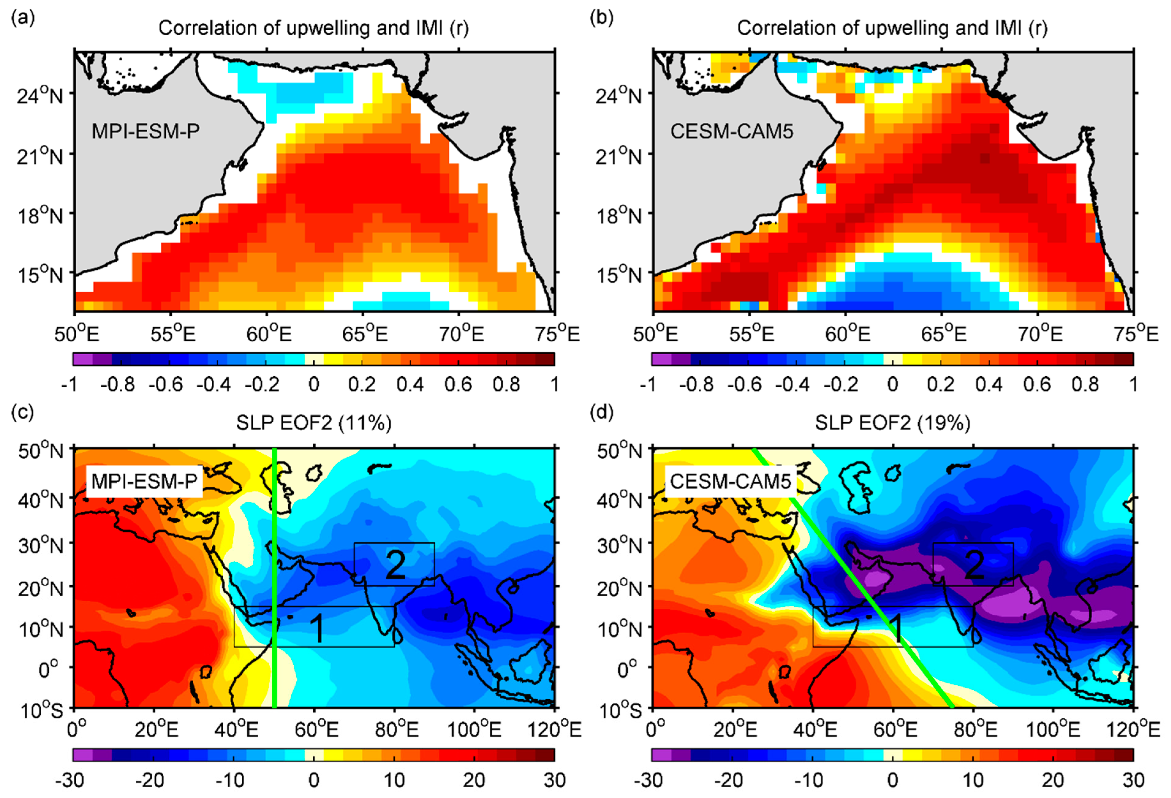
It is shown in Figure 5a,b that the IMI is also correlated to the upwelling velocity in the rest of the coastal areas in the Arabian Sea and the negative correlation in the central downwelling region indicates that the IMI contributes to the intensification of the downwelling as well. Since the IMI is calculated based on the wind field, which is caused by the sea level pressure (SLP) gradient, we also applied the EOF analysis to the SLP field. We find that the time series of the coastal upwelling in the western Arabian Sea from both of the models are also significantly correlated with the PC time series of the second mode from the EOF analysis of the SLP (Table 1).
This EOF mode of SLP displays a clear spatial pattern representing the contrast between Africa and Indo-Asia (Figure 5c,d). In general, the patterns revealed from the two models are very similar. However, the boundary line, which separates the positive and negative EOF phases, rotates anticlockwise in CESM-CAM5 comparing to that in MPI-ESM-P. This tilt might be responsible for the 8% more variance captured by the second EOF mode of SLP from CESM-CAM5 than that from MPI-ESM-P as well as the higher correlation between the SLP PC2 and the coastal upwelling time series derived from CESM-CAM5 than that from MPI-ESM-P (Table 1). An explanation might be that, with this tilt, the second EOF mode revealed from CESM-CAM5 captures a contrast of the spatial patterns in the southern Arabian Sea that contributes to the variance representing the SW wind-stress, which highly correlates with the time series of the coastal upwelling in the western Arabian Sea.
3.3. Upwelling Trends
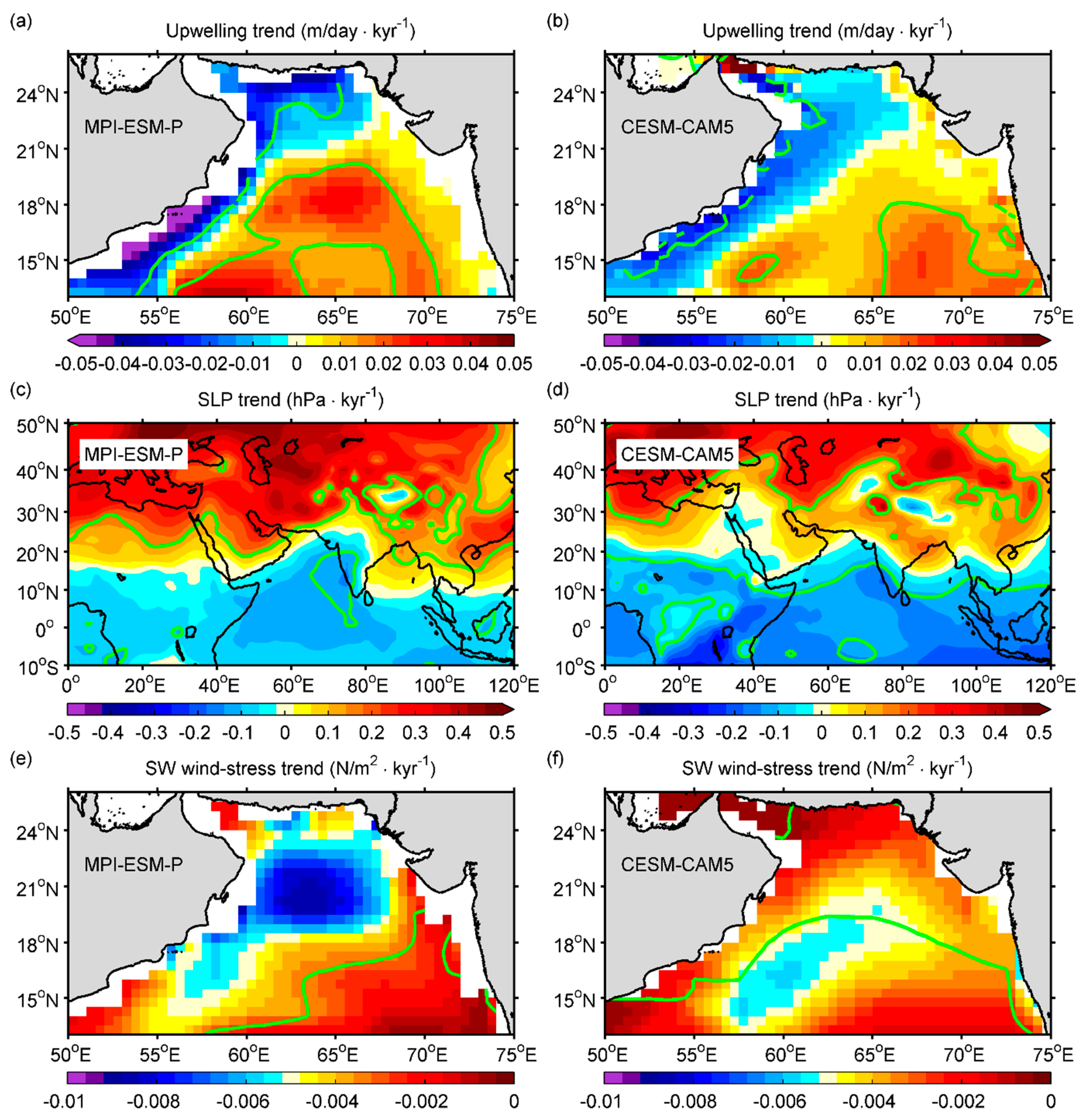
In order to understand the millennial scale variability of the Arabian Sea upwelling, we calculated the long-term linear trends of the vertical velocity and determined their significance level using the Mann–Kendall test. Figure 6a,b shows the upwelling trends derived from the two simulations. Both models reveal negative trends in the northern Arabian Sea and along the coast where the intense upwelling occurs. On the contrary, the central and eastern Arabian Seas display positive trends. Note that the central Arabian Sea is dominated by downwelling, and so the positive trends in this region actually indicate a weakening of downwelling, whereas in the eastern Arabian Sea the upwelling is slightly strengthened. However, in the western Arabian Sea, the region of our main focus, the upwelling velocity decreased over the last millennium, whereby the MPI-ESM-P model displays a more significant reduction than the CESM-CAM5 model. The upwelling velocity trends share very similar spatial patterns with the first mode of MPI-ESM-P (Figure 3a) and the second mode of CESM-CAM5 (Figure 3d) from the EOF analysis. In addition, their PC time series (Figure 4a,d) also confirm the trends revealed in the upwelling velocity time series (Figure 1c,d). The different signs in the EOF spatial patterns and the trends in the PC time series indicate the weakening of the western Arabian Sea coastal upwelling. The trends revealed from the time series are small in terms of their amplitudes over a thousand years compared to the mean upwelling velocity. However, negative trends of western Arabian Sea upwelling are shown consistently in all the six simulations by the two models despite the different internal conditions used for the simulations. Thus, the overall picture of these trends is highly statistically significant, which is determined by applying a classical sign test [46]. The sign test is usually applied in statistical climatology, for instance, Tebaldi et al. [48] employed this method to test the significance level of the precipitation trends simulated in an ensemble of climate simulations. In our case, the fact that all the six simulations reveal negative trends leads to a strong overall significance, not to mention that the trends are not only all negative, but some are also statistically significant at the individual p = 0.05 level. Therefore, the weakening of upwelling in this region is very likely a robust feature in the simulations.
These trends are likely induced by the external forcing used to drive the models. Among all the external forcings, only the orbital forcing displays the long-term millennial scale trend, so that the identified upwelling trends can presumably be attributed to the orbital forcing. The change in orbital forcing is a significant cause of the SST trends revealed in the tropical and subtropical regions [49]. It contributes to the increased land–sea thermal contrast, which enhances the SLP gradient between land and ocean. As a result, the monsoon was strengthened during the Mid-Holocene [50]. More recently, Gill et al. [51] have shown negative trends of the Arabian Sea upwelling and the Indian Monsoon from past to present, which is also linked to the orbital forcing.
To confirm the effect of the orbital forcing, we calculated the trends of the SLP (Figure 6c,d) and the SW wind-stress (Figure 6e,f) since the upwelling is mainly forced by the SW wind-stress, which is generated from the SLP gradient. The spatial patterns of the SLP trends show clearly that in mid latitudes the SLP tends to increase and in low latitudes the SLP tends to decrease. These patterns are quite likely resulting from the effect of orbital forcing, as similar long-term changes are also derived from the differences between equilibrium mid-Holocene and present climate simulations [52]. For the last millennium, Lücke et al. [53] have recently found that the trends in the climate models can be attributed to the orbital forcing.
Moreover, we also compared our results with those from the individual forcing experiments (orbital-forcing-only and solar-forcing-only) of the CESM-CAM5 model. It is found that both upwelling and SLP in the orbital-forcing-only simulations present similar trend patterns as what is shown in Figure 6 but they are not revealed from the solar-forcing-only simulations. This further ascertains the impact of the orbital forcing. With positive trends in the mid latitudes and negative trends in the low latitudes, the SLP contrast between these areas is reduced, which further affects the wind in the Arabian Sea. During the summer upwelling season, this SLP contrast drives the SW wind so when the SLP contrast is reduced, the SW wind is also weakened. Figure 6e,f presents the negative trends of SW wind-stress as expected. In general, the trend from MPI-ESM-P is larger than that from CESM-CAM5. Since the western Arabian Sea coastal upwelling is significantly linked to the SW wind-stress in the Arabian Sea, the negative trends of SW wind-stress can cause the decrease in the upwelling velocity (Figure 6a,b). A larger trend of SW wind-stress in the case of the MPI-ESM-P model than in the CESM-CAM5 model also results in stronger trend of upwelling. Therefore, the weakening of the coastal upwelling in the western Arabian Sea is induced by the reduction of the SW wind-stress, which results from the long-term change of the SLP contrast between mid and low latitudes due to the orbital forcing.
3.4. Future Scenarios
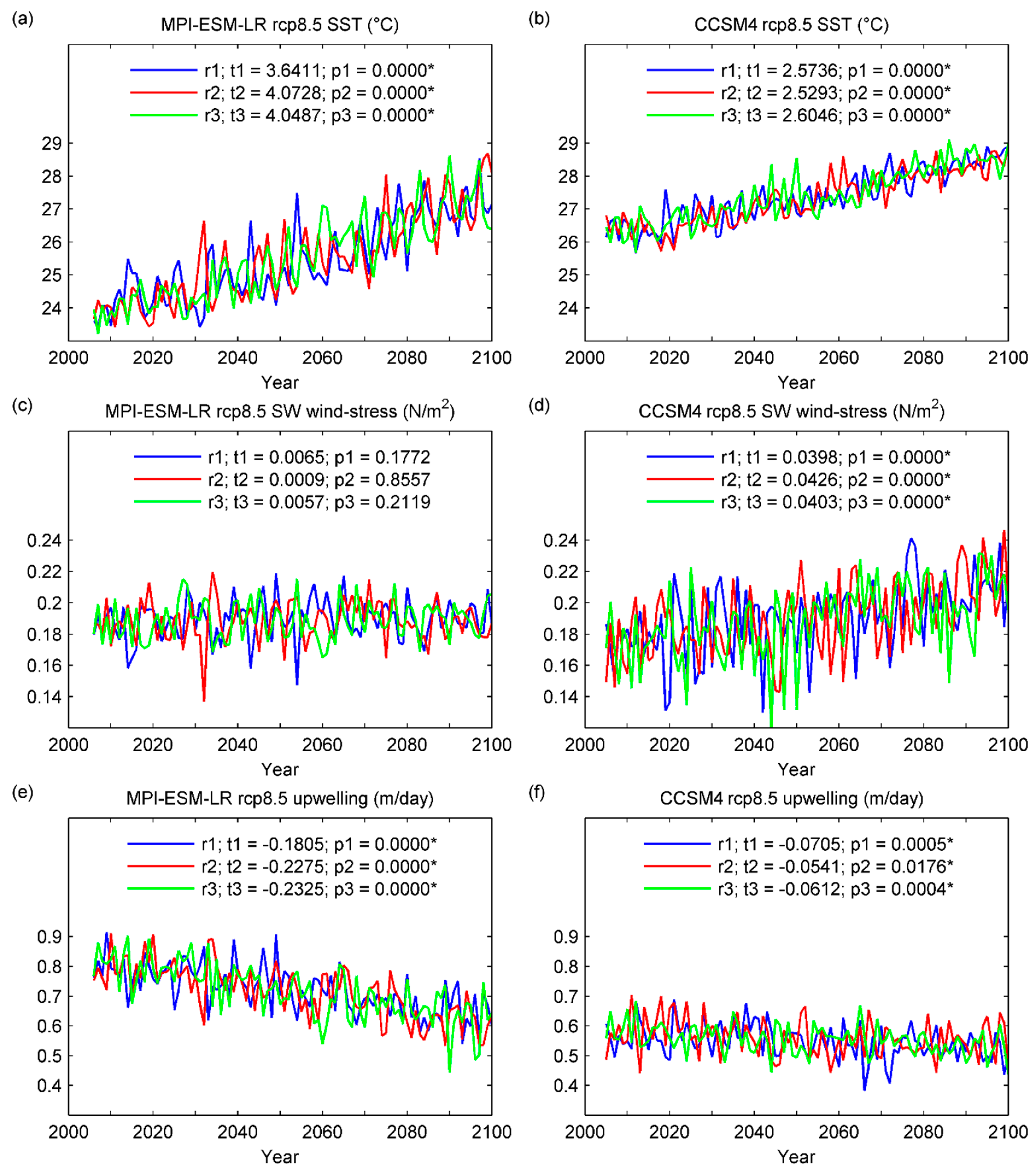
In addition to the analyses of the last millennium simulations, we studied the trends in the future scenarios as well. Figure 7 presents the time series of the SST, the SW wind-stress and the upwelling velocity modeled by MPI-ESM-LR and CCSM4 under the scenario RCP8.5. In order to be consistent with the last millennium study, these time series were calculated from the same selected area shown in Figure 1.
All the simulations by the two models are quite consistent regarding the results for the RCP8.5 scenario by showing positive trends in SST and SW wind-stress but negative trends in upwelling velocity. The SST (Figure 7a,b) increases significantly under the effect of the greenhouse gas emission. In the MPI-ESM-LR model (Figure 7a) the SST begins with lower values than that in the CCSM4 model (Figure 7b) but they rise to similar values by the end of the simulations, so the SST modeled by the MPI-ESM-LR has a larger trend than the CCSM4. The SW wind-stress (Figure 7c,d) is also strengthened due to the enhanced contrast between the surface heating over the land and the sea. This finding of enhanced upwelling favorable winds is consistent with the result of Menon et al. [54]. They presented that the simulated changes in the Monsoon circulation are quite robust across the CMIP model ensemble and consistent with the changes simulated by the MPI-ESM and CESM models, including the strengthening of the upwelling favorable winds in the future under RCP8.5 scenario. Although all the simulations by both models show positive trends, the CCSM4 simulations (Figure 7d) reveal more distinct and significant trends than the MPI-ESM-LR (Figure 7c). As a result of the intensification of the wind-stress, the upwelling velocity is expected to increase as well. However, negative trends of upwelling velocity are found in all the simulations (Figure 7e,f) especially for the MPI-ESM-LR (Figure 7e). In addition, we also examined the simulated upwelling in the CESM model under the RCP8.5 scenario in the 21st century and it shows similar results as in the CCSM4 model with significant trends at the same order, despite the differences between two models. Therefore, an interesting question arises as to what is causing the negative trend in upwelling velocity given that the upwelling favorable wind-stress is projected to increase. Figure 7 indicates that with stronger trends in SST and weaker trends in SW wind-stress, the MPI-ESM-LR simulations present a stronger decrease in upwelling whereas the CCSM4 simulated upwelling decreases less as the SST reveals weaker trends and the SW wind-stress shows stronger trends in CCSM4. Thus, it is likely that the increase in surface water stratification caused by warming of the upper ocean layers in the RCP8.5 scenario could override the effect of the upwelling favorable wind. The upwelling weakens more when the warming is stronger or the wind is less intensified, and vice versa.
This hypothesis is confirmed by the results simulated under the RCP2.6 scenario where both models show weaker warming of surface water than the RCP8.5 simulations but no consistent trend in the SW wind-stress or the upwelling. That is, without the strong increase in SST the water stratification in the upper layers is less intense so the decrease in upwelling is weaker and is compromised by the effect of the SW wind-stress. Note that the correlations between the upwelling and the SW wind-stress are similar in RCP8.5 and RCP2.6 scenarios (Table 2) so the influences of the wind on the upwelling are at the same level.
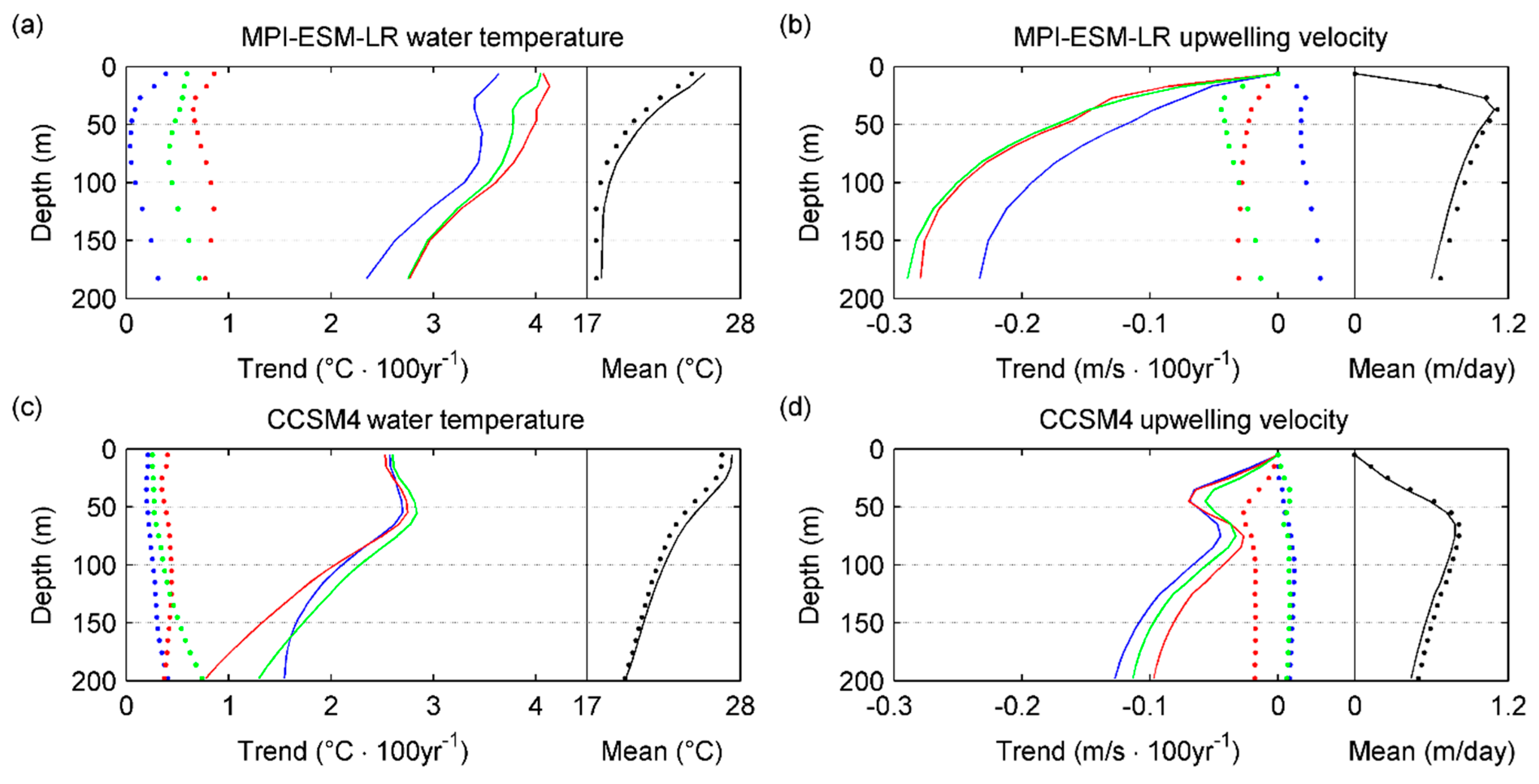
In addition, Figure 8 presents the trends of upwelling velocity and water temperature at all levels in the upper 200 m, which further supports that the upwelling reduction under RCP8.5 scenario is caused by the surface water stratification due to the strong warming. It is very clear, especially in the CCSM4 plots (Figure 8c,d), that in the upper 50–100 m the upwelling velocity shows larger negative trends when the trends of the water temperature increase. At around 50 m depth, the temperature trends reach their peaks and the upwelling trends also get to the lowest values (in the surface layer above 100 m). The upwelling is actually most intense at this layer, but it is most reduced as well, which causes the drop in the upwelling time series shown in Figure 7. Therefore, in spite of the positive correlation between the SW wind-stress and the upwelling, the warming of the upper ocean layers under the RCP8.5 scenario reduces the upwelling velocity more efficiently.
4. Discussion
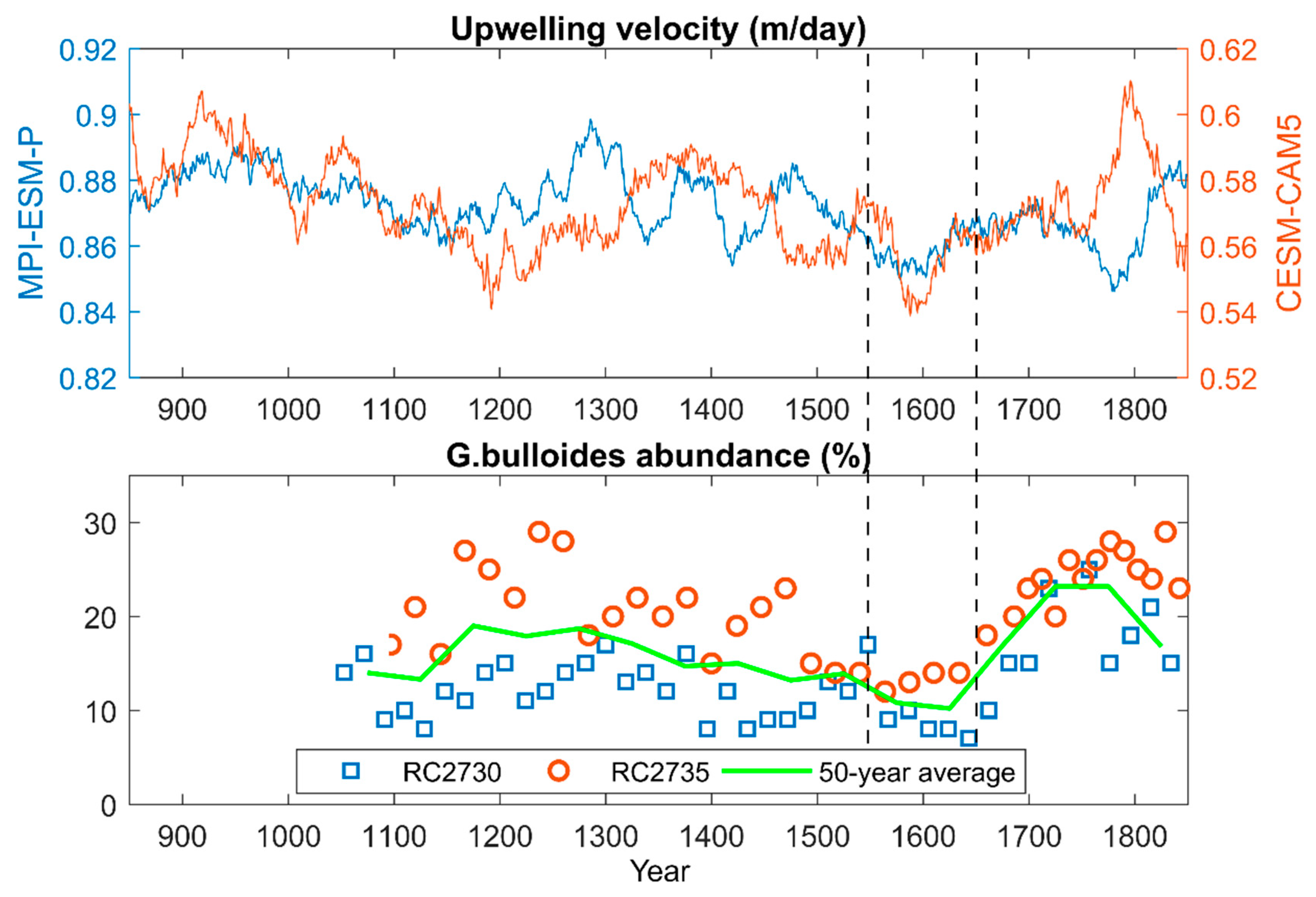
One limitation of this study is that it relies to a great extent on the realism of the models employed, which makes it very difficult to validate the results as there are no available direct observations on upwelling over the time span. However, we do find a connection between our modeled upwelling velocity and the observational sediment records. They present a significant correlation (Figure 2), which indicates the effect of the external forcing. In addition, they also have similar patterns in the time series in terms of the trends. It can be noticed that the long-term trend revealed from the upwelling time series (Figure 1) tends to flip, especially in the CESM-CAM5 model, at around the year 1550. This flip was reported by Anderson et al. [15] where they reconstructed the upwelling index (monsoon winds) from the sediment records over the last millennium. They found a slightly negative trend from 1000 to 1500 and a positive trend thereafter, which is very similar to our finding. Thus, we divided our upwelling time series into two periods based on the flip and calculated the trends separately (Table 3).
It is very clear that five out of six of the simulations indicate a flip in the long-term trend at 1550 as the signs of the trends change from negative to positive after this point (except for the CESM-CAM5 r1), which is at about the same time as the G. bulloides records. This is also shown when comparing the upwelling time series with the replot of the data from Anderson et al. [15] presented in Figure 9.
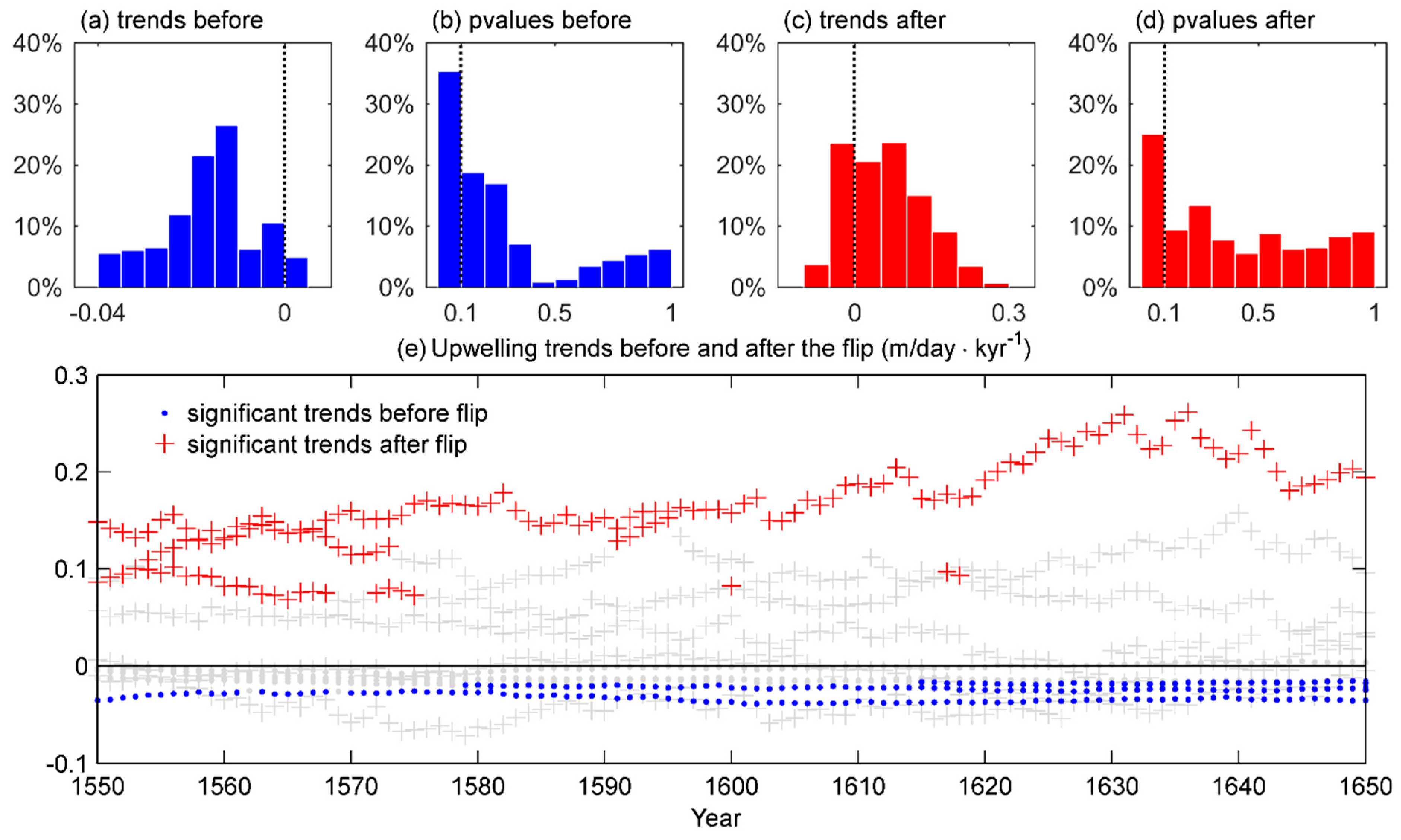
To explore the flip in the modeled upwelling time series, we selected a range of years from 1550 to 1650 when the flip might happen. We considered each of the years within this range as a flip point and calculated the trends before and after this point, that is, the trend from 850 to the selected year and the trend from the selected year to 1850. We applied this to all the six simulations of the MPI-ESM-P and the CESM-CAM5 models and combined the results. The histograms in Figure 10 show that 95% of the trends before the flip point are negative and 73% of the trends after the flip point are positive. Among all the trends before and after the flip point, the percentage of the significant (p-value < 0.1) ones are 35% and 25%, respectively. More importantly, the significant trends are consistent on the signs in both cases (negative before flip and positive after flip). Therefore, the models produce realistic upwelling time series that agree with the observational sediment records. However, uncertainties remain as the exact time when the trends change signs varies from simulation to simulation, which might be caused by the different initial conditions applied for each simulation.
Model resolution also has an impact on the realism of the results [55,56]. However, it is still unclear what resolution is most suitable to model the Arabian Sea coastal upwelling system. In our study, the MPI-ESM uses a coarser horizontal resolution (256 × 220) than the CESM (320 × 384) and produces the upwelling velocity with larger means but less variability, as well as larger trends. The upwelling velocity simulated by the CESM, however, has stronger correlation with the wind and the wind based IMI. Whether these differences are caused by the different resolutions is uncertain, but this comparison might shed light on how the modeled Arabian Sea upwelling responds to the change in the model resolutions.
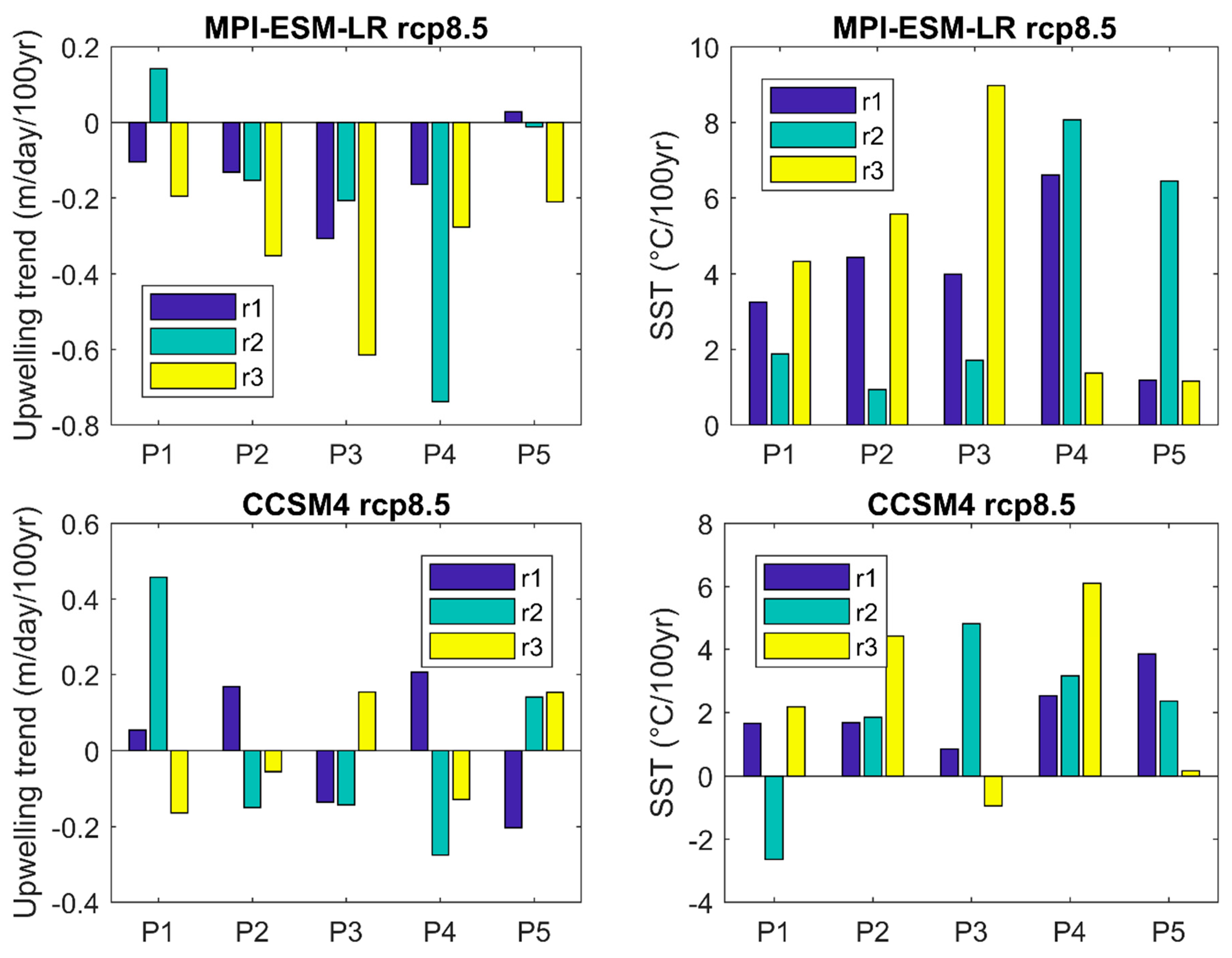
A recent study found a reduction in the future upwelling at low latitudes in most of the four EBUSs [18]. In our analysis for the future scenario RCP8.5, the upwelling velocity also reveals a negative trend whereas the SW wind-stress presents a positive trend. Thus, the reduction of the upwelling is not caused by the wind-stress, although they are still significantly correlated. The analysis for the RCP2.6 scenario does not show a trend in either the upwelling or the SW wind-stress, but it shows strong correlation between upwelling and the wind-stress as well as the RCP8.5 scenario. Wang et al. [18] suggested several mechanisms that could lead to a reduction in the upwelling at low latitudes such as strengthened downwelling favorable winds, weakened upwelling favorable winds, and enhanced water stratification due to the greenhouse warming. More specifically, Roxy et al. [57] looked into the simulated chlorophyll concentrations and found out a drop of marine phytoplankton during the last 60 years due to the enhanced ocean stratification, which shows a similar mechanism to our case. The stratified water under the RCP8.5 scenario reduces the upwelling, however, this is not shown in the RCP2.6 scenario. Although both models used in the present study show the overriding effect of the water stratification for the RCP8.5 scenario, their future decadal trends are not mutually consistent (Figure 11). Whereas this effect exists for all the simulations of the MPI-ESM-LR model since the beginning of the 21st century and reaches maxima during 2044 to 2081, the CCSM4 model does not show the same results. Therefore, it remains for further study to investigate at what level of future emissions between the strongest and the weakest warming scenarios the water stratification and the effect of wind-stress approximately balance.
5. Conclusions
The variability of the Arabian Sea upwelling over the last millennium and in the 21st century was investigated in this study. We statistically analyzed and compared the outputs of four earth system model simulation ensembles. Over the last millennium, the modeled upwelling velocity has a strong correlation with the SST and the IMI as well as the observed G.bulloides abundance. This indicates a close connection among the Arabian Sea upwelling, the Indian summer Monsoon and the sediment records. A negative long-term trend is found in the upwelling velocity over the last millennium, which is resulting from the orbital forcing of the models. In the last 300 years, however, the upwelling reveals a positive trend that matches the observations in the sediment records. As for the future scenarios, the correlation between upwelling and the SW wind-stress remains at the same level under the RCP8.5 and RCP2.6 scenarios but the stronger greenhouse gas emission scenario leads to opposite trends in the SW wind-stress and the upwelling velocity. The positive trend in the SW wind-stress is caused by the intensified SLP gradient between land and ocean due to the warming effect. The upwelling velocity shows a negative trend because under the stronger scenario, the warming of the sea water tends to stabilize the surface layer, which overrides the effect of the SW wind-stress and interrupts the upwelling.
Author Contributions
Conceptualization, X.Y., B.H. and E.Z.; methodology, X.Y. and E.Z.; validation, X.Y. and B.H.; formal analysis, X.Y.; investigation, X.Y.; writing—original draft preparation, X.Y.; writing—review and editing, X.Y., B.H. and E.Z.; visualization, X.Y.; supervision, B.H. and E.Z. All authors have read and agreed to the published version of the manuscript.
Funding
This research received no external funding.
Data Availability Statement
The model outputs are within the CMIP5 model pool and are available from https://pcmdi.llnl.gov/mips/cmip5/data-portal.html (accessed on 17 March 2021). The G. bulloides records from Anderson et al. [15] can be accessed at ftp://ftp.ncdc.noaa.gov/pub/data/paleo/contributions_by_author/anderson2002/anderson2002.txt (accessed on 17 March 2021).
Acknowledgments
This paper is a contribution to the Cluster of Excellence “Climate, Climatic Change, and Society” (CLICCS). We thank the Max-Planck-Institute for Meteorology for providing the MPI-ESM model data. All the other publicly available data used in this study are gratefully acknowledged.
Conflicts of Interest
The authors declare no conflict of interest.
References
- Pauly, D.; Christensen, V. Primary production required to sustain global fisheries. Nature 1995, 374, 255–257. [Google Scholar] [CrossRef]
- Izumo, T.; Montégut, C.B.; Luo, J.-J.; Behera, S.K.; Masson, S.; Yamagata, T. The Role of the Western Arabian Sea Upwelling in Indian Monsoon Rainfall Variability. J. Clim. 2008, 21, 5603–5623. [Google Scholar] [CrossRef] [Green Version]
- Bakun, A. Global Climate Change and Intensification of Coastal Ocean Upwelling. Science 1990, 247, 198–201. [Google Scholar] [CrossRef] [PubMed] [Green Version]
- Schwing, F.B.; Mendelssohn, R. Increased coastal upwelling in the California Current System. J. Geophys. Res. Oceans 1997, 102, 3421–3438. [Google Scholar] [CrossRef]
- McGregor, H.V.; Dima, M.; Fischer, H.W.; Mulitza, S. Rapid 20th-Century Increase in Coastal Upwelling off Northwest Africa. Science 2007, 315, 637–639. [Google Scholar] [CrossRef] [PubMed]
- Gutiérrez, D.; Bouloubassi, I.; Sifeddine, A.; Purca, S.; Goubanova, K.; Graco, M.; Field, D.; Méjanelle, L.; Velazco, F.; Lorre, A.; et al. Coastal cooling and increased productivity in the main upwelling zone off Peru since the mid-twentieth century. Geophys. Res. Lett. 2011, 38, L07603. [Google Scholar] [CrossRef] [Green Version]
- Santos, F.; Gomez-Gesteira, M.; deCastro, M.; Alvarez, I. Differences in coastal and oceanic SST trends due to the strengthening of coastal upwelling along the Benguela current system. Cont. Shelf Res. 2012, 34, 79–86. [Google Scholar] [CrossRef]
- Narayan, N.; Paul, A.; Mulitza, S.; Schulz, M. Trends in coastal upwelling intensity during the late 20th century. Ocean Sci. 2010, 6, 815–823. [Google Scholar] [CrossRef] [Green Version]
- Sydeman, W.J.; García-Reyes, M.; Schoeman, D.S.; Rykaczewski, R.R.; Thompson, S.A.; Black, B.A.; Bograd, S.J. Climate change and wind intensification in coastal upwelling ecosystems. Science 2014, 345, 77–80. [Google Scholar] [CrossRef]
- Bauer, S.; Hitchcock, G.L.; Olson, D.B. Influence of monsoonally-forced Ekman dynamics upon surface layer depth and plankton biomass distribution in the Arabian Sea. Deep Sea Res. Part A Oceanogr. Res. Pap. 1991, 38, 531–553. [Google Scholar] [CrossRef]
- Anderson, D.M.; Prell, W.L. A 300 KYR Record of Upwelling Off Oman during the Late Quaternary: Evidence of the Asian Southwest Monsoon. Paleoceanography 1993, 8, 193–208. [Google Scholar] [CrossRef]
- Sirocko, F.; Sarnthein, M.; Lange, H.; Erlenkeuser, H. Atmospheric summer circulation and coastal upwelling in the Arabian Sea during the Holocene and the last glaciation. Quat. Res. 1991, 36, 72–93. [Google Scholar] [CrossRef]
- Leuschner, D.C.; Sirocko, F. Orbital insolation forcing of the Indian Monsoon—A motor for global climate changes? Palaeogeogr. Palaeoclimatol. Palaeoecol. 2003, 197, 83–95. [Google Scholar] [CrossRef]
- Anderson, D.M.; Baulcomb, C.K.; Duvivier, A.K.; Gupta, A.K. Indian summer monsoon during the last two millennia. J. Quat. Sci. 2010, 25, 911–917. [Google Scholar] [CrossRef]
- Anderson, D.M.; Overpeck, J.T.; Gupta, A.K. Increase in the Asian Southwest Monsoon During the Past Four Centuries. Science 2002, 297, 596–599. [Google Scholar] [CrossRef] [PubMed]
- Feng, S.; Hu, Q. Regulation of Tibetan Plateau heating on variation of Indian summer monsoon in the last two millennia. Geophys. Res. Lett. 2005, 32. [Google Scholar] [CrossRef]
- Sinha, A.; Berkelhammer, M.; Stott, L.; Mudelsee, M.; Cheng, H.; Biswas, J. The leading mode of Indian Summer Monsoon precipitation variability during the last millennium. Geophys. Res. Lett. 2011, 38, L15703. [Google Scholar] [CrossRef] [Green Version]
- Wang, D.; Gouhier, T.C.; Menge, B.A.; Ganguly, A.R. Intensification and spatial homogenization of coastal upwelling under climate change. Nature 2015, 518, 390–394. [Google Scholar] [CrossRef]
- Taylor, K.E.; Stouffer, R.J.; Meehl, G.A. An Overview of CMIP5 and the Experiment Design. Bull. Am. Meteorol. Soc. 2012, 93, 485–498. [Google Scholar] [CrossRef] [Green Version]
- Moss, R.H.; Edmonds, J.A.; Hibbard, K.A.; Manning, M.R.; Rose, S.K.; van Vuuren, D.P.; Carter, T.R.; Emori, S.; Kainuma, M.; Kram, T.; et al. The next generation of scenarios for climate change research and assessment. Nature 2010, 463, 747–756. [Google Scholar] [CrossRef]
- Tim, N.; Zorita, E.; Hünicke, B.; Yi, X.; Emeis, K.C. The importance of external climate forcing for the variability and trends of coastal upwelling in past and future climate. Ocean Sci. 2016, 12, 807–823. [Google Scholar] [CrossRef] [Green Version]
- Edwards, P.N. A Vast Machine: Computer Models, Climate Data, and the Politics of Global Warming; MIT Press: Cambridge, MA, USA, 2010. [Google Scholar]
- Giorgetta, M.A.; Jungclaus, J.; Reick, C.H.; Legutke, S.; Bader, J.; Böttinger, M.; Brovkin, V.; Crueger, T.; Esch, M.; Fieg, K.; et al. Climate and carbon cycle changes from 1850 to 2100 in MPI-ESM simulations for the Coupled Model Intercomparison Project phase 5. J. Adv. Model. Earth Syst. 2013, 5, 572–597. [Google Scholar] [CrossRef]
- Otto-Bliesner, B.L.; Brady, E.C.; Fasullo, J.; Jahn, A.; Landrum, L.; Stevenson, S.; Rosenbloom, N.; Mai, A.; Strand, G. Climate Variability and Change since 850 CE: An Ensemble Approach with the Community Earth System Model. Bull. Am. Meteorol. Soc. 2016, 97, 735–754. [Google Scholar] [CrossRef]
- Hurrell, J.W.; Holland, M.M.; Gent, P.R.; Ghan, S.; Kay, J.E.; Kushner, P.J.; Lamarque, J.-F.; Large, W.G.; Lawrence, D.; Lindsay, K.; et al. The Community Earth System Model: A Framework for Collaborative Research. Bull. Am. Meteorol. Soc. 2013, 94, 1339–1360. [Google Scholar] [CrossRef]
- Masson-Delmotte, V.; Schulz, M.; Abe-Ouchi, A.; Beer, J.; Ganopolski, A.; González Rouco, J.F.; Jansen, E.; Lambeck, K.; Luterbacher, J.; Naish, T.; et al. Information from paleoclimate archives. In Climate Change 2013: The Physical Science Basis. Contribution of Working Group I to the Fifth Assessment Report of the Intergovernmental Panel on Climate Change; Stocker, T.F., Qin, D., Plattner, G.-K., Tignor, M., Allen, S.K., Boschung, J., Nauels, A., Xia, Y., Bex, V., Midgley, P.M., Eds.; Cambridge University Press: Cambridge, UK; New York, NY, USA, 2013; pp. 383–464. [Google Scholar]
- Vieira, L.E.A.; Solanki, S.K. Evolution of the solar magnetic flux on time scales of years to millenia. Astron. Astrophys. 2010, 509, A100. [Google Scholar] [CrossRef]
- Berger, A. Long-Term Variations of Daily Insolation and Quaternary Climatic Changes. J. Atmos. Sci. 1978, 35, 2362–2367. [Google Scholar] [CrossRef]
- Gao, C.; Robock, A.; Ammann, C. Volcanic forcing of climate over the past 1500 years: An improved ice core-based index for climate models. J. Geophys. Res. Atmos. 2008, 113, D23111. [Google Scholar] [CrossRef] [Green Version]
- Crowley, T.J.; Unterman, M.B. Technical details concerning development of a 1200 yr proxy index for global volcanism. Earth Syst. Sci. Data 2013, 5, 187–197. [Google Scholar] [CrossRef] [Green Version]
- Pongratz, J.; Raddatz, T.; Reick, C.H.; Esch, M.; Claussen, M. Radiative forcing from anthropogenic land cover change since A.D. 800. Geophys. Res. Lett. 2009, 36, L02709. [Google Scholar] [CrossRef] [Green Version]
- Flückiger, J.; Monnin, E.; Stauffer, B.; Schwander, J.; Stocker, T.F.; Chappellaz, J.; Raynaud, D.; Barnola, J.-M. High-resolution Holocene N2O ice core record and its relationship with CH4 and CO2. Glob. Biogeochem. Cycles 2002, 16. [Google Scholar] [CrossRef]
- Hansen, J.; Sato, M. Greenhouse gas growth rates. Proc. Natl. Acad. Sci. USA 2004, 101, 16109–16114. [Google Scholar] [CrossRef] [Green Version]
- MacFarling Meure, C.; Etheridge, D.; Trudinger, C.; Steele, P.; Langenfelds, R.; van Ommen, T.; Smith, A.; Elkins, J. Law Dome CO2, CH4 and N2O ice core records extended to 2000 years BP. Geophys. Res. Lett. 2006, 33, L14810. [Google Scholar] [CrossRef]
- Brock, J.C.; McClain, C.R. Interannual variability in phytoplankton blooms observed in the northwestern Arabian Sea during the southwest monsoon. J. Geophys. Res. Oceans 1992, 97, 733–750. [Google Scholar] [CrossRef]
- Brock, J.C.; McClain, C.R.; Luther, M.E.; Hay, W.W. The phytoplankton bloom in the northwestern Arabian Sea during the southwest monsoon of 1979. J. Geophys. Res. Oceans 1991, 96, 20623–20642. [Google Scholar] [CrossRef]
- Rixen, T.; Haake, B.; Ittekkot, V. Sedimentation in the western Arabian Sea the role of coastal and open-ocean upwelling. Deep Sea Res. Part II Top. Stud. Oceanogr. 2000, 47, 2155–2178. [Google Scholar] [CrossRef]
- Shi, W.; Morrison, J.M.; Böhm, E.; Manghnani, V. The Oman upwelling zone during 1993, 1994 and 1995. Deep Sea Res. Part II Top. Stud. Oceanogr. 2000, 47, 1227–1247. [Google Scholar] [CrossRef]
- Yi, X.; Hünicke, B.; Tim, N.; Zorita, E. The relationship between Arabian Sea upwelling and Indian Monsoon revisited in a high resolution ocean simulation. Clim. Dyn. 2018, 50, 201–213. [Google Scholar] [CrossRef] [Green Version]
- Thadathil, P.; Thoppil, P.; Rao, R.R.; Muraleedharan, P.M.; Somayajulu, Y.K.; Gopalakrishna, V.V.; Murtugudde, R.; Reddy, G.V.; Revichandran, C. Seasonal Variability of the Observed Barrier Layer in the Arabian Sea. J. Phys. Oceanogr. 2008, 38, 624–638. [Google Scholar] [CrossRef] [Green Version]
- Lee, C.M.; Jones, B.H.; Brink, K.H.; Fischer, A.S. The upper-ocean response to monsoonal forcing in the Arabian Sea: Seasonal and spatial variability. Deep Sea Res. Part II Top. Stud. Oceanogr. 2000, 47, 1177–1226. [Google Scholar] [CrossRef]
- Turner, A.G.; Joshi, M.; Robertson, E.S.; Woolnough, S.J. The effect of Arabian Sea optical properties on SST biases and the South Asian summer monsoon in a coupled GCM. Clim. Dyn. 2012, 39, 811–826. [Google Scholar] [CrossRef]
- Lévy, M.; Shankar, D.; André, J.M.; Shenoi, S.S.C.; Durand, F.; de Boyer Montégut, C. Basin-wide seasonal evolution of the Indian Ocean’s phytoplankton blooms. J. Geophys. Res. Oceans 2007, 112, C12014. [Google Scholar] [CrossRef] [Green Version]
- Peeters, F.J.C.; Brummer, G.-J.A.; Ganssen, G. The effect of upwelling on the distribution and stable isotope composition of Globigerina bulloides and Globigerinoides ruber (planktic foraminifera) in modern surface waters of the NW Arabian Sea. Glob. Planet. Chang. 2002, 34, 269–291. [Google Scholar] [CrossRef]
- Ebisuzaki, W. A Method to Estimate the Statistical Significance of a Correlation When the Data Are Serially Correlated. J. Clim. 1997, 10, 2147–2153. [Google Scholar] [CrossRef]
- von Storch, H.; Zwiers, F.W. Statistical Analysis in Climate Research; Cambridge University Press: Cambridge, UK, 2001. [Google Scholar]
- Wang, B.; Fan, Z. Choice of South Asian Summer Monsoon Indices. Bull. Am. Meteorol. Soc. 1999, 80, 629–638. [Google Scholar] [CrossRef] [Green Version]
- Tebaldi, C.; Arblaster, J.M.; Knutti, R. Mapping model agreement on future climate projections. Geophys. Res. Lett. 2011, 38, L23701. [Google Scholar] [CrossRef]
- Lorenz, S.J.; Kim, J.-H.; Rimbu, N.; Schneider, R.R.; Lohmann, G. Orbitally driven insolation forcing on Holocene climate trends: Evidence from alkenone data and climate modeling. Paleoceanography 2006, 21, PA1002. [Google Scholar] [CrossRef]
- Jiang, D.; Lang, X.; Tian, Z.; Ju, L. Mid-Holocene East Asian summer monsoon strengthening: Insights from Paleoclimate Modeling Intercomparison Project (PMIP) simulations. Palaeogeogr. Palaeoclimatol. Palaeoecol. 2013, 369, 422–429. [Google Scholar] [CrossRef]
- Gill, E.C.; Rajagopalan, B.; Molnar, P.H.; Kushnir, Y.; Marchitto, T.M. Reconstruction of Indian summer monsoon winds and precipitation over the past 10,000 years using equatorial pacific SST proxy records. Paleoceanography 2017, 32, 195–216. [Google Scholar] [CrossRef]
- Braconnot, P.; Loutre, M.; Dong, B.; Joussaume, S.; Valdes, P. How the simulated change in monsoon at 6 ka BP is related to the simulation of the modern climate: Results from the Paleoclimate Modeling Intercomparison Project. Clim. Dyn. 2002, 19, 107–121. [Google Scholar] [CrossRef]
- Lücke, L.J.; Schurer, A.P.; Wilson, R.; Hegerl, G.C. Orbital Forcing Strongly Influences Seasonal Temperature Trends During the Last Millennium. Geophys. Res. Lett. 2021, 48, e2020GL088776. [Google Scholar] [CrossRef]
- Menon, A.; Levermann, A.; Schewe, J.; Lehmann, J.; Frieler, K. Consistent increase in Indian monsoon rainfall and its variability across CMIP-5 models. Earth Syst. Dynam. 2013, 4, 287–300. [Google Scholar] [CrossRef] [Green Version]
- Small, R.J.; Curchitser, E.; Hedstrom, K.; Kauffman, B.; Large, W.G. The Benguela Upwelling System: Quantifying the Sensitivity to Resolution and Coastal Wind Representation in a Global Climate Model. J. Clim. 2015, 28, 9409–9432. [Google Scholar] [CrossRef]
- Ranjha, R.; Tjernström, M.; Svensson, G.; Semedo, A. Modelling coastal low-level wind-jets: Does horizontal resolution matter? Meteorol. Atmos. Phys. 2016, 128, 263–278. [Google Scholar] [CrossRef]
- Roxy, M.K.; Modi, A.; Murtugudde, R.; Valsala, V.; Panickal, S.; Prasanna Kumar, S.; Ravichandran, M.; Vichi, M.; Lévy, M. A reduction in marine primary productivity driven by rapid warming over the tropical Indian Ocean. Geophys. Res. Lett. 2016, 43, 826–833. [Google Scholar] [CrossRef] [Green Version]
Figure 1.
Spatial patterns of JJA mean Arabian Sea upwelling velocity modeled by (a) MPI-ESM-P and (b) CESM-CAM5. Time series of JJA coastal upwelling velocity in the western Arabian Sea modeled by (c) MPI-ESM-P and (d) CESM-CAM5. The area selected for calculating the variable time series is shown in (a,b) within the green line. The plotted time series are smoothed by a 31-year moving mean window and r1, r2, r3 represent the three simulations. t1, t2, t3 are the trends (per 1000 years) of each simulation with p1, p2 and p3 indicating their p-values, respectively, and the star symbols mark the simulations that pass the significance test at the 95% level.

Figure 2.
Correlation coefficient between the SST and the upwelling velocity modeled by (a) MPI-ESM-P and (b) CESM-CAM5 with significance level greater than 95% (p-value < 0.05). Correlation coefficient between the G. bulloides abundance and the upwelling velocity simulated by (c) MPI-ESM-P and (d) CESM-CAM5. The green point marks the location of the sediment core where the G. bulloides abundance is recorded. The regions surrounded by the green contour lines present significant correlations that are at a higher level than 90% (p-value < 0.1). All the correlation coefficients are calculated from the detrended time series.

Figure 3.
First EOF mode of JJA Arabian Sea upwelling velocity modeled by (a) MPI-ESM-P and (b) CESM-CAM5 and second EOF mode from (c) MPI-ESM-P and (d) CESM-CAM5 with their explained variance in brackets.
Figure 3.
First EOF mode of JJA Arabian Sea upwelling velocity modeled by (a) MPI-ESM-P and (b) CESM-CAM5 and second EOF mode from (c) MPI-ESM-P and (d) CESM-CAM5 with their explained variance in brackets.

Figure 4.
First principal component (PC) time series corresponding to the first EOF mode for all the simulation in (a) MPI-ESM-P and (b) CESM-CAM5 and second PC time series of (c) MPI-ESM-P and (d) CESM-CAM5. The plotted PCs are smoothed by a 31-year moving mean window and r1, r2, r3 represent the three simulations. t1, t2, t3 are the trends (per 1000 years) of each simulation with p1, p2 and p3 indicating their p-values, respectively, and the star symbols mark the simulations that pass the significance test at the 95% level.

Figure 5.
Correlation coefficient between the upwelling velocity and the IMI modeled by (a) MPI-ESM-P and (b) CESM-CAM5. The IMI is calculated by subtracting the U850 wind averaged in box2 from that in box1 (boxes shown in c,d). All the correlation coefficients are calculated from the detrended time series and are significant at the 95% significance level. The second EOF mode of JJA SLP modeled by (c) MPI-ESM-P and (d) CESM-CAM5 with their explained variance in brackets. The green lines demonstrate approximately the simplified boundaries that divide the positive and negative EOF phases.

Figure 6.
Long-term trends of JJA upwelling velocity modeled by (a) MPI-ESM-P and (b) CESM-CAM5. Long-term trends of JJA SLP modeled by (c) MPI-ESM-P and (d) CESM-CAM5. Long-term trends of JJA SW wind-stress in the Arabian Sea modeled by (e) MPI-ESM-P and (f) CESM-CAM5. The regions surrounded by the green contour lines present significant trends that are at a higher level than 90% (p-value < 0.1).

Figure 7.
Time series of (a) SST, (c) SW wind-stress and (e) upwelling velocity modeled by MPI-ESM-LR under the scenario of RCP8.5 for the 21st century. (b,d,f) are the same variables respectively modeled by CCSM4. r1, r2, r3 represent the three simulations of each model. t1, t2, t3 are the trends (per 100 years) of each simulation with p1, p2 and p3 indicating their p-values, respectively, and the star symbols mark the simulations that pass the significance test at the 95% level.

Figure 8.
Vertical trends of (a) water temperature and (b) upwelling velocity in the upper 200 m modeled by MPI-ESM-LR. (c,d) are the same but by CCSM4. Solid lines are the results for the RCP8.5 scenario and dotted lines are for the RCP2.6 scenario. The colored lines show the trends of r1 (blue), r2 (red), and r3 (green) in each model. The black lines on the right of each panel present the mean value of the current variable.

Figure 9.
Upwelling velocity modeled by MPI-ESM-P (blue) and CESM-CAM5 (red) for the last millennium (upper) and replotted using data of Anderson et al. (2002) for the G. bulloides abundance (lower). The blue and red markers show the data from two sediment records located very closely in the western Arabian Sea, RC2730 and RC2735, respectively. The green line is the average of all the records in a block of 50 years. The dashed black lines show the period where the “flip” is detected.

Figure 10.
Histograms of (a) trends and (b) p-values for the period before the selected flip point. Histograms of (c) trends and (d) p-values for the period after the selected flip point. (e) Trends before (dot) and after (plus) each flip point from 1550 to 1650. The colored markers show significant trends with p-value < 0.1.

Figure 11.
Decadal trends for the future RCP 8.5 scenario in the MPI-ESM-LR (upper) and CCSM4 (lower) models for upwelling (left) and SST (right). P1 to P5 represent the 19-year periods from 2006 to 2100.
Figure 11.
Decadal trends for the future RCP 8.5 scenario in the MPI-ESM-LR (upper) and CCSM4 (lower) models for upwelling (left) and SST (right). P1 to P5 represent the 19-year periods from 2006 to 2100.


Table 1.
Correlation coefficient between the coastal upwelling velocity in the western Arabian Sea and the Indian Monsoon Index (IMI), the upwelling PCs *, the SLP PC2, and the G. bulloides abundance for all the six simulations from the two models. All the correlation coefficients are calculated from the detrended time series and are significant at the 95% significance level except for the G. bulloides where only the second simulation of MPI-ESM-P presents the significant correlation.
| MPI-ESM-P Upwelling TS | CESM-CAM5 Upwelling TS | |||||
|---|---|---|---|---|---|---|
| r1 | r2 | r3 | r1 | r2 | r3 | |
| IMI | 0.64 | 0.61 | 0.60 | 0.64 | 0.66 | 0.65 |
| Upwelling PCs * | 0.79 | 0.85 | 0.83 | 0.92 | 0.93 | 0.93 |
| SLP PC2 | 0.61 | 0.50 | 0.55 | 0.84 | 0.87 | 0.83 |
| G. bulloides | 0.14 | 0.66 | −0.06 | −0.27 | 0.07 | 0.21 |
* Upwelling PC2 is used for correlations within the MPI-ESM-P simulations but upwelling PC1 is used for CESM-CAM5.
Table 2.
Correlation coefficient between the upwelling velocity and the SW wind-stress modeled by MPI-ESM-LR and CCSM4 for the RCP8.5 and RCP2.6 scenarios. All the correlation coefficients are calculated from the detrended time series and are significant at the 95% significance level.
Table 2.
Correlation coefficient between the upwelling velocity and the SW wind-stress modeled by MPI-ESM-LR and CCSM4 for the RCP8.5 and RCP2.6 scenarios. All the correlation coefficients are calculated from the detrended time series and are significant at the 95% significance level.
| MPI-ESM-LR | CCSM4 | |||||
|---|---|---|---|---|---|---|
| r1 | r2 | r3 | r1 | r2 | r3 | |
| RCP8.5 | 0.5457 | 0.4787 | 0.5420 | 0.4844 | 0.5500 | 0.5321 |
| RCP2.6 | 0.4270 | 0.4259 | 0.4752 | 0.7569 | 0.6391 | 0.6879 |
Table 3.
Upwelling trends (m/day per 1000 years) calculated from the two models for different time periods: the entire time period (850–1849), the first 700 years (850–1549), and the last 300 years (1550–1849).
Table 3.
Upwelling trends (m/day per 1000 years) calculated from the two models for different time periods: the entire time period (850–1849), the first 700 years (850–1549), and the last 300 years (1550–1849).
| MPI-ESM-P Upwelling Trend | CESM-CAM5 Upwelling Trend | |||||
|---|---|---|---|---|---|---|
| r1 | r2 | r3 | r1 | r2 | r3 | |
| 850–1849 | −0.0187 * | −0.0062 | −0.0164 * | −0.0013 | −0.0129 | −0.0138 |
| 850–1549 | −0.0120 | −0.0052 | −0.0105 | −0.0005 | −0.0028 | −0.0343 * |
| 1550–1849 | 0.0567 | 0.0862 * | 0.0062 | −0.0100 | 0.1484 * | 0.0905 |
* Trends that are significant at the 95% level.
Publisher’s Note: MDPI stays neutral with regard to jurisdictional claims in published maps and institutional affiliations. |
© 2021 by the authors. Licensee MDPI, Basel, Switzerland. This article is an open access article distributed under the terms and conditions of the Creative Commons Attribution (CC BY) license (https://creativecommons.org/licenses/by/4.0/).
Share and Cite
MDPI and ACS Style
Yi, X.; Hünicke, B.; Zorita, E. Evolution of the Arabian Sea Upwelling from the Last Millennium to the Future as Simulated by Earth System Models. Climate 2021, 9, 72. https://0-doi-org.brum.beds.ac.uk/10.3390/cli9050072
AMA Style
Yi X, Hünicke B, Zorita E. Evolution of the Arabian Sea Upwelling from the Last Millennium to the Future as Simulated by Earth System Models. Climate. 2021; 9(5):72. https://0-doi-org.brum.beds.ac.uk/10.3390/cli9050072
Chicago/Turabian StyleYi, Xing, Birgit Hünicke, and Eduardo Zorita. 2021. "Evolution of the Arabian Sea Upwelling from the Last Millennium to the Future as Simulated by Earth System Models" Climate 9, no. 5: 72. https://0-doi-org.brum.beds.ac.uk/10.3390/cli9050072
Note that from the first issue of 2016, this journal uses article numbers instead of page numbers. See further details here.