Global Surface Temperature: A New Insight


1
Department of Civil and Environmental Engineering and Water Resources Research Center, University of Hawaii at Manoa, Honolulu, HI 96822, USA
2
Department of Civil and Environmental Engineering, College of Engineering, Chung-Ang University, Seoul 06974, Korea
*
Author to whom correspondence should be addressed.
Climate 2021, 9(5), 81; https://0-doi-org.brum.beds.ac.uk/10.3390/cli9050081
Submission received: 27 April 2021
/
Accepted: 7 May 2021
/
Published: 12 May 2021
(This article belongs to the Special Issue Application of Climatic Data in Hydrologic Models)
This paper belongs to our Special Issue “Application of Climate Data in Hydrologic Models”. Here, we represent an example of the importance of climate data in terms of global surface temperature. This paper investigates the changes of 20-year (2000–2019) mean surface temperature (ST), wind speed (WS), and albedo (AL) data from the Global Land Data Assimilation System (GLDAS) over the globe with respect to those in 1961–1990. Moreover, we assess if the alterations in ST are affected by the changes in WS and AL. We also discuss the main reasons for the variations observed in ST, WS, and AL on global and hemispheric scales.
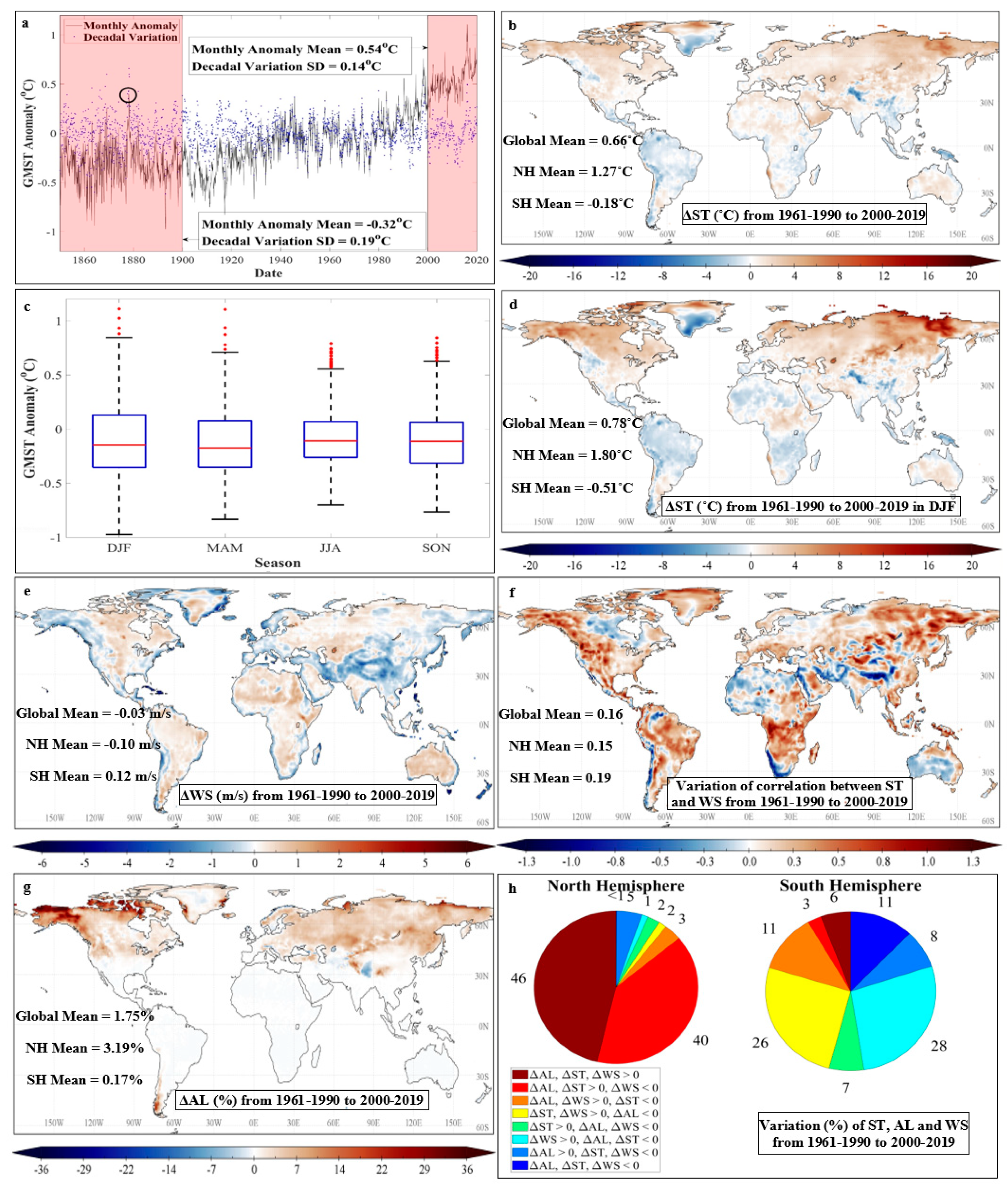
Our planet is within ~1 °C of its highest surface temperature in the past million years [1]. The most important indicator of global warming and climate change is the global mean surface temperature (GMST) [2]. Figure 1a shows the time series of monthly GMST anomalies from the Hadly Center/Climate Research Unit (HadCRUT) [2,3]. The mean of monthly GMST anomalies in 2000–2019 is 0.54 °C higher than that in 1961–1990 (Figure 1a) (see also [1,4]). The standard deviation (SD) of the decadal variation of GMST anomalies is reduced by 0.05 °C in 2000–2019 compared to 1850–1899 (Figure 1a). This is due to the climate sensitivity to oscillation indices, particularly El Niño/Southern Oscillation (ENSO) [5]. Indeed, there were more ENSO events in 1850–1900 than in 2000–2020, which affected the GMST anomalies. For example, the high positive GMST anomaly in 1878 (shown by the black circle) is caused by the late 1870s El Niño (Figure 1a) [1].
Figure 1b shows the variation of Global Land Data Assimilation System (GLDAS) ST data (ΔST) from 1961–1990 to 2000–2019 over the globe. The results show the GMST increase of 0.66 °C from 1961–1990 to 2000–2019. Analogously, Hansen et al. [1] reported the GMST growth of ~0.2 °C per decade during the last three decades. As indicated in Figure 1b, in general, the Northern Hemisphere (NH) has a higher variation of ST (ΔST) than the Southern Hemisphere (SH) [4]. The averages of ΔST in the NH and SH are 1.27 °C and −0.18 °C, respectively. Increasing greenhouse gas (GHG) emissions and variations of the North Atlantic Oscillation (NAO) are the main causes of increasing ST across the globe and particularly in the NH [1,6]. Effective policies must focus on using clean energies to reduce the GHG emissions. Such policies can facilitate achieving the 2015 Paris COP21 Agreement to maintain the GMST below 1.5–2 °C above pre-industrial levels. The decreasing ST in the SH is associated with the variations of the SH Annular Mode (SAM) and intensification of the South Pacific Anticyclone [7,8]. Fogt and Marshall [7] showed that adiabatic cooling over the Antarctica due to the variations of SAM aids in decreasing ST in the SH.
Figure 1c indicates the boxplot of GMST anomalies in each season. The horizontal line within the box indicates the median. The upper and lower edges of the box represent the 75% and 25% percentiles, respectively. The upper and lower ends of the whiskers show the maximum and minimum values, respectively. Outliers are observations beyond the end of the whiskers. As shown, the variation of the GMST anomaly during December–February (DJF) is more than that of other seasons. Vose et al. [9] also observed the highest upward decadal trend of ST in the NH (particularly high latitudes) in DJF when the minimum ST often occurs. In addition, the global minimum ST has increased approximately twice as fast as the global maximum ST since 1950 [9]. Hence, a larger variation in the GMST anomaly is seen in DJF (Figure 1c).
Comparison of Figure 1b,d illustrates a larger variation of ST during DJF in both hemispheres. During DJF, the mean of ΔST in the NH is 1.8 °C (Figure 1d). However, in some parts of Eastern Russia, it can reach up to 20 °C (Figure 1d). Hansen et al. [1] concluded that the global warming of more than ~1 °C could lead to a dangerous climate change and impacts the sea water level.
From 1961–1990 to 2000–2019, the GLDAS ST (WS) increased (decreased) in the northwest of North America (Alaska) and northeast of Asia (Russia) (Figure 1b,e). Both ST and WS increased in Canada (except in the western part), most regions of Australia and North Africa. In most regions of Africa and South America, WS enhanced, but ST reduced. Figure 1f shows the changes in the ST-WS correlation () from 1961–1990 to 2000–2019. High positive or negative values of (>1 or <−1) in Southern Africa, North Greenland, Western America, Eastern Russia, and Central and Eastern Asia denote the changes of vegetation cover [10].
As can be seen in Figure 1e, winds slow down in most of the coastal regions as well as in Central and Eastern of Asia due to an increase in the surface roughness. These findings are consistent with those of Vautard et al. [10] who reported the highest downward trend of WS in Central and Eastern Asia from 1979 to 2008 due to the land-use change and/or biomass increase. They demonstrated that increasing the Normalized Difference Vegetation Index (NDVI) in Eurasia could explain 25–60% of the NH atmospheric stilling.
The increase of AL plays an important role in future climate change [11]. Ghimire et al. [12] reported an increase of about 1% in the global albedo due to the land cover change during 1700–2005. That caused the global atmospheric radiation to vary by almost 0.15 W/m2. Figure 1g represents changes in the GLDAS AL from 1961–1999 to 2000–2019 over the globe. On average, AL increases by 3.19% in the NH. AL varies with changes in cloud fractional coverage, aerosol amount, and land cover type [13]. If the variation of AL is caused by changes in aerosols and land cover type, ST reduces by rising AL [13]. In the NH, AL increased from 1961–1999 to 2000–2019 (Figure 1g), while ST did not decrease (Figure 1b). Therefore, the increase of AL is indicative of climatologically significant cloud-induced variations in the Earth’s radiation budget, which is in line with the GMST growth in recent decades [11]. Another reason of AL growth may be the intensified wildfires in the NH boreal forests (due to droughts), especially in Canada and Alaska (see also [14,15]). In this region, the ST increase (Figure 1b,d) along with the precipitation reduction led to drought, which enhanced the wildfire severity [14].
Through changing ST, NDVI, AL and evapotranspiration, wildfire is the dominant driver of water, energy, and carbon cycles as well as vegetation dynamics in the North American boreal region [15,16]. The aforementioned region has the highest increase of AL that can reach up to 36% (Figure 1g). Likewise, Jin et al. [16] indicated that the increased severity of wildfires in the North American boreal forests during 2000–2009 enhanced AL by ~60%. Potter et al. [15] showed that climate change counteracts the cooling impact of postfire AL growth in the NH boreal forests. This justifies the increase of ST despite rising AL in the NH (Figure 1b,g).
Figure 1h compares the changes of ST, WS, and AL from 1961–1990 to 2000–2009 in the NH and SH. Both ST and AL increased in 86% of the NH and 9% of SH regions. Increase of ST in most regions on the NH leads to drought events, which intensify wildfires, ultimately rising AL. In addition, variations of ST are consistent with those of WS (i.e., both increase or decrease) in 53% and 51% of the areas of NH and SH, respectively. This happens because WS can affect ST through modifying evapotranspiration [17,18].
Regional studies are necessary to improve our understanding of the variations in ST, WS, and AL [4]. Some important regions for further investigations are the High Mountains of Asia, which demonstrate extreme values of ΔST (Figure 1b), ΔWS (Figure 1e), and ΔAL (Figure 1g) (see also [10,19]).
At the end, we would like to thank all the authors for their contributions to this Special Issue. We hope that the papers published in this Special Issue improve our knowledge in terms of application of climate data in hydrologic models.
Author Contributions
Conceptualization, M.V.; investigation, M.V., S.M.B., C.J.; writing—original draft preparation, M.V.; writing—review and editing, S.M.B., C.J., supervision, S.M.B., C.J. All authors have read and agreed to the published version of the manuscript.
Funding
This research received no external funding.
Institutional Review Board Statement
Not applicable.
Informed Consent Statement
Not applicable.
Data Availability Statement
The data that support the findings of this study are available from the corresponding authors upon reasonable request.
Conflicts of Interest
The authors declare no conflict of interest.
References
- Hansen, J.; Sato, M.; Ruedy, R.; Lo, K.; Lea, D.W.; Medina-Elizade, M. Global temperature change. Proc. Natl. Acad. Sci. USA 2006, 103, 14288–14293. [Google Scholar] [CrossRef] [PubMed] [Green Version]
- Foster, G.; Rahmstorf, S. Global temperature evolution 1979–2010. Environ. Res. Lett. 2011, 6, 044022. [Google Scholar] [CrossRef]
- Hawkins, E.; Ortega, P.; Suckling, E.; Schurer, A.; Hegerl, G.; Jones, P.; Joshi, M.; Osborn, T.J.; Masson-Delmotte, V.; Mignot, J.; et al. Estimating changes in global temperature since the preindustrial period. Bull. Am. Meteorol. Soc. 2017, 98, 1841–1856. [Google Scholar] [CrossRef]
- Huntingford, C.; Jones, P.D.; Livina, V.N.; Lenton, T.M.; Cox, P.M. No increase in global temperature variability despite changing regional patterns. Nature 2013, 500, 327–330. [Google Scholar] [CrossRef] [PubMed]
- Nijsse, F.J.; Cox, P.M.; Huntingford, C.; Williamson, M.S. Decadal global temperature variability increases strongly with climate sensitivity. Nat. Clim. Chang. 2019, 9, 598–601. [Google Scholar] [CrossRef]
- Wang, X.; Li, J.; Sun, C.; Liu, T. NAO and its relationship with the Northern Hemisphere mean surface temperature in CMIP5 simulations. J. Geophys. Res. Atmos. 2017, 122, 4202–4227. [Google Scholar] [CrossRef]
- Fogt, R.L.; Marshall, G.J. The Southern Annular Mode: Variability, trends, and climate impacts across the Southern Hemisphere. Wiley Interdiscip. Rev. Clim. Chang. 2020, 11, e652. [Google Scholar] [CrossRef]
- Falvey, M.; Garreaud, R.D. Regional cooling in a warming world: Recent temperature trends in the southeast Pacific and along the west coast of subtropical South America (1979–2006). J. Geophys. Res Atmos. 2009, 114, D04102. [Google Scholar] [CrossRef]
- Vose, R.S.; Easterling, D.R.; Gleason, B. Maximum and minimum temperature trends for the globe: An update through 2004. Geophysic. Res. Lett. 2005, 32, L23822. [Google Scholar] [CrossRef] [Green Version]
- Vautard, R.; Cattiaux, J.; Yiou, P.; Thépaut, J.N.; Ciais, P. Northern Hemisphere atmospheric stilling partly attributed to an increase in surface roughness. Nat. Geosci. 2010, 3, 756–761. [Google Scholar] [CrossRef]
- Pallé, E.; Goode, P.R.; Montanes-Rodriguez, P.; Koonin, S.E. Changes in Earth’s reflectance over the past two decades. Science 2004, 304, 1299–1301. [Google Scholar] [CrossRef] [PubMed] [Green Version]
- Ghimire, B.; Williams, C.A.; Masek, J.; Gao, F.; Wang, Z.; Schaaf, C.; He, T. Global albedo change and radiative cooling from anthropogenic land cover change, 1700 to 2005 based on MODIS, land use harmonization, radiative kernels, and reanalysis. Geophys. Res. Lett. 2014, 41, 9087–9096. [Google Scholar] [CrossRef]
- Wielicki, B.A.; Wong, T.; Loeb, N.; Minnis, P.; Priestley, K.; Kandel, R. Changes in Earth’s albedo measured by satellite. Science 2005, 308, 825. [Google Scholar] [CrossRef] [PubMed]
- Xiao, J.; Zhuang, Q. Drought effects on large fire activity in Canadian and Alaskan forests. Environ. Res. Lett. 2007, 2, 044003. [Google Scholar] [CrossRef]
- Potter, S.; Solvik, K.; Erb, A.; Goetz, S.J.; Johnstone, J.F.; Mack, M.C.; Randerson, J.T.; Roman, M.O.; Schaaf, C.L.; Turetsky, M.R.; et al. Climate change decreases the cooling effect from postfire albedo in boreal North America. Glob. Chang. Biol. 2020, 26, 1592–1607. [Google Scholar] [CrossRef] [PubMed]
- Jin, Y.; Randerson, J.T.; Goetz, S.J.; Beck, P.S.; Loranty, M.M.; Goulden, M.L. The influence of burn severity on postfire vegetation recovery and albedo change during early succession in North American boreal forests. J. Geophys. Res. Biogeosci. 2012, 117. [Google Scholar] [CrossRef]
- Sheffield, J.; Wood, E.F.; Roderick, M.L. Little change in global drought over the past 60 years. Nature 2012, 491, 435–438. [Google Scholar] [CrossRef] [PubMed]
- Valipour, M.; Bateni, S.M.; Gholami Sefidkouhi, M.A.; Raeini-Sarjaz, M.; Singh, V.P. Complexity of forces driving trend of reference evapotranspiration and signals of climate change. Atmosphere 2020, 11, 1081. [Google Scholar] [CrossRef]
- Kraaijenbrink, P.D.; Bierkens MF, P.; Lutz, A.F.; Immerzeel, W.W. Impact of a global temperature rise of 1.5 degrees Celsius on Asia’s glaciers. Nature 2017, 549, 257–260. [Google Scholar] [CrossRef]
- HadCRUT. 2021. Available online: https://crudata.uea.ac.uk/cru/data/temperature/ (accessed on 10 May 2021).
- GES DISC. 2021. Available online: https://disc.gsfc.nasa.gov/ (accessed on 10 May 2021).
Figure 1.
(a); Time series of monthly and decadal GMST anomalies. The 1850–1899 and 2000–2019 periods are shown by pink colors to compare the variations before the 20th century and after the 21st century, (b); variation of the GMST, (c); boxplots of the GMST anomalies. The horizontal line within the box indicates the median (50% percentile). The upper and lower edges of the box represent the 75% and 25% percentile, respectively. The upper and lower ends of the whiskers represent the maximum and minimum values. Outliers are observations beyond the end of the whiskers, (d); variation of the GMST in DJF, (e); variation of WS, (f); variation of the correlation between the GMST and WS, (g); variation of AL, (h); Hemispheric variation of the GMST, AL and WS. (a,c) are plotted based on the HadCRUT-version 4.6 product [20]. (b,d–h) are drawn based on the GLDAS (1° × 1° spatial resolution and monthly temporal resolution) dataset [21].

Publisher’s Note: MDPI stays neutral with regard to jurisdictional claims in published maps and institutional affiliations. |
© 2021 by the authors. Licensee MDPI, Basel, Switzerland. This article is an open access article distributed under the terms and conditions of the Creative Commons Attribution (CC BY) license (https://creativecommons.org/licenses/by/4.0/).
Share and Cite
MDPI and ACS Style
Valipour, M.; Bateni, S.M.; Jun, C. Global Surface Temperature: A New Insight. Climate 2021, 9, 81. https://0-doi-org.brum.beds.ac.uk/10.3390/cli9050081
AMA Style
Valipour M, Bateni SM, Jun C. Global Surface Temperature: A New Insight. Climate. 2021; 9(5):81. https://0-doi-org.brum.beds.ac.uk/10.3390/cli9050081
Chicago/Turabian StyleValipour, Mohammad, Sayed M. Bateni, and Changhyun Jun. 2021. "Global Surface Temperature: A New Insight" Climate 9, no. 5: 81. https://0-doi-org.brum.beds.ac.uk/10.3390/cli9050081
Note that from the first issue of 2016, this journal uses article numbers instead of page numbers. See further details here.