
Bottom-Up Drivers for Global Fish Catch Assessed with Reconstructed Ocean Biogeochemistry from an Earth System Model


1
Department of Environmental Engineering and Energy, Myongji University, Yongin-si 17058, Korea
2
Department of Earth and Environmental Sciences, Jeonbuk National University, Jeollabuk-do 54896, Korea
3
Department of Environment and Energy, Jeonbuk National University, Jeollabuk-do 54896, Korea
*
Author to whom correspondence should be addressed.
Climate 2021, 9(5), 83; https://0-doi-org.brum.beds.ac.uk/10.3390/cli9050083
Submission received: 11 March 2021
/
Revised: 6 May 2021
/
Accepted: 11 May 2021
/
Published: 14 May 2021
(This article belongs to the Special Issue The Resilience and Adaptation of Aquatic Ecosystem’s Structure and Function to Climate Change)
Abstract
:Identifying bottom-up (e.g., physical and biogeochemical) drivers for fish catch is essential for sustainable fishing and successful adaptation to climate change through reliable prediction of future fisheries. Previous studies have suggested the potential linkage of fish catch to bottom-up drivers such as ocean temperature or satellite-retrieved chlorophyll concentration across different global ecosystems. Robust estimation of bottom-up effects on global fisheries is, however, still challenging due to the lack of long-term observations of fisheries-relevant biotic variables on a global scale. Here, by using novel long-term biological and biogeochemical data reconstructed from a recently developed data assimilative Earth system model, we newly identified dominant drivers for fish catch in globally distributed coastal ecosystems. A machine learning analysis with the inclusion of reconstructed zooplankton production and dissolved oxygen concentration into the fish catch predictors provides an extended view of the links between environmental forcing and fish catch. Furthermore, the relative importance of each driver and their thresholds for high and low fish catch are analyzed, providing further insight into mechanistic principles of fish catch in individual coastal ecosystems. The results presented herein suggest the potential predictive use of their relationships and the need for continuous observational effort for global ocean biogeochemistry.
1. Introduction
Climate-driven changes in marine physical and biogeochemical states significantly impact life in the ocean [1,2,3]. Albeit with large uncertainty in regional patterns, state-of-the-art Earth system models (ESMs) project future warming, acidification, deoxygenation and reduced productivity [4], all of which are known to modify marine habitat distributions, phenologies, and consequently change the functioning of marine ecosystems [5,6,7,8]. These environmental changes inevitably affect fisheries production, and thus require adaptive fisheries management in response to climate-driven environmental changes. Given stagnating world fish catch even with expanding worldwide fishing effort and its socioeconomic impacts on human society, future changes in fisheries production and their potential predictability are of particular interest to many scientific communities, policy makers, and fishery industries.
Historical fish catch variation is known to be affected by both top-down and bottom-up factors or a combination of them. Top-down factors include fishing effort and harvest control. Pacific sardine fishery demise in the 1950s and the collapse of the Peruvian anchoveta fishery in the 1970s are examples of fisheries production affected by human factors, despite the high sensitivity of their production to changes in bottom-up drivers [9,10]. Bottom-up factors affecting fisheries production include ocean temperature, phytoplankton biomass, and dissolved oxygen concentration. Ocean temperature and chlorophyll, as a proxy for complex changes in recruitment variability, trophic dynamics, and spawning habitat availability, are acknowledged to be major bottom-up drivers explaining historical fisheries production in many large coastal areas of global oceans [11,12,13]. Particularly, globally observed sea surface temperature explains historical fisheries productions in many high latitude regions and can be utilized to predict fish catch and to set optimal harvest guidelines [11,14,15]. Previous studies also suggested that the relative strength of human and environmental factors varies in space and time and their interactions are important for historical fish catch variations [16].
Global observational data are an indispensable requirement to evaluate the relationship between bottom-up drivers and fisheries production on a basin or global scale. Physical variables such as ocean temperature and salinity are globally available due to well-established global observational platforms, thus their relationship to fisheries production across different marine ecosystems is well documented in the aforementioned studies. In contrast, climate-driven variability of marine biogeochemical and biological variables and its influence on fisheries production are less documented due to the lack of global observations of those variables. Satellited-retrieved chlorophyll-a estimates (a proxy for phytoplankton biomass) since the late 1970s are one of the most important global marine biogeochemistry observations and the only means of estimating phytoplankton chlorophyll concentrations on a global scale, enabling a series of attempts to explain and predict fisheries production [11,17,18,19]. However, the earlier satellite chlorophyll data are severely limited in tropical regions and there is a consistency issue when directly calibrating with contemporary data [20]. Therefore, a consistent chlorophyll data set spans ~20 years and using these data only may not be enough to elucidate a rigorous linkage between environmental drivers and fish catch. Moreover, there are other bottom-up drivers of fisheries, which are potentially better indicators for fish catch estimation but have not been observed on a global scale. For example, mesozooplankton production represents the food web process to sustain populations [12,21], and dissolved oxygen also modifies fish metabolic rates and viable habitats [3].
In this study, we used the reconstructed ocean states from a data assimilative Earth system model product, taking advantage of globally available ocean biological and biogeochemical variables such as mesozooplankton production and dissolved oxygen concentration. Using these 24-year-long data together with ocean temperature, we identified regions where the bottom-up drivers predominate historical fish catch variations in large coastal areas of the global ocean. We also examined the relative importance of those drivers for fish catch across different marine ecosystems.
2. Data and Methods
2.1. Reconstructed Ocean Physical-Biogeochemical Field
The historical ocean states (i.e., physical, biological, and biogeochemical variables) used in this study were generated following a previous work [22]. First, the ESM developed at GFDL (Geophysical Fluid Dynamics Laboratory) in the NOAA (National Oceanic and Atmospheric Administration) was coupled to GFDL’s ensemble coupled data assimilation (ECDA) system that has been used for GFDL’s operational seasonal forecasts [23]. Observed physical states in the atmosphere and ocean were then assimilated into the ESM and reproduced historical ocean state variables for the period 1991–2017, in which the first 24-year data are only used in this study to match with the fish catch data. Here, we assimilated 6 hourly winds and temperature from NCEP-DOE (National Centers for Environmental Prediction, Department of Energy) Reanalysis 2 product for the atmosphere [24], while for the ocean we assimilated NOAA optimum interpolation sea surface temperature v2 high-resolution data, oceanic profiles from the World Ocean Database (WOD), Argo, and global temperature-salinity profile program (GTSPP) data sets [25,26,27]. Note that biological and biogeochemical variables were not assimilated into the data assimilation system due to the lack of their global observations. Instead, those biotic variables were indirectly updated by the data assimilative physics within the ESM. That is, given that biological and biogeochemical variables in the ocean are, in general, sensitively controlled by physical states, improved physical ocean states by assimilating observed temperature and salinity provides a constraint that helps to reduce the bias of biotic variables simulated from the biogeochemical model. The ECDA system employed an ensemble Kalman filter with 12 ensemble members to estimate the probability distribution function of climate states.
One of the key elements to successfully estimate global biogeochemistry in the present study is the biogeochemical model incorporated into GFDL’s ESM, named as the Carbon, Ocean Biogeochemistry and Lower Trophics (COBALT) [28]. COBALT is the most complex biogeochemical model from a hierarchy of GFDL’s biogeochemical models and it considers 33 tracers, including phytoplankton, zooplankton, organic and inorganic matters, to resolve global-scale cycles of dissolved organic/inorganic matters and three phytoplankton and zooplankton groups. COBALT has been implemented in different versions of ESMs and tested against a diverse set of observations including nutrients and planktonic food web flux estimates. Simulated marine biogeochemistry by this model has been shown to capture the observed large-scale mean patterns as well as the site-by-site means, being ranked highly among Coupled Model Intercomparison Project (CMIP)-class Earth system models [29]. Previous studies also showed that GFDL’s ESM and its coupled version with the ECDA system successfully reproduced historical biogeochemical variables [22,30]. For example, as shown in Figure 1, the mean of ocean biological and biogeochemical variables (such as nitrate, dissolved oxygen, and chlorophyll concentration) simulated from our data assimilative model run shows good agreement with the long-term mean globally observed data from WOD (for nitrate and oxygen) and the satellite-based ocean color sensors (for chlorophyll), Sea-viewing Wide Field-of-view Sensor and Moderate Resolution Imaging Spectroradiometer [31,32]. The detailed performance of the assimilative model used in this study is documented in a previous work, including the comparison with a non-assimilative run in terms of the mean and variability of ocean biogeochemistry [22].
2.2. Fisheries Production Data
To analyze the relationship between bottom-up factors (i.e., temperature (°C), mesozooplankton production (mol m−2 s−1), and dissolved oxygen (mol kg−1)) and fish catch (tonnage), we obtained annual mean fisheries yield data provided by the Sea Around Us project [33]. The data consist of the aggregated fish catches that are from bottom trawl, purse seine, pelagic trawl, longline, gillnet and other unknown sources, and they provide reconstructed fisheries production in coastal Large Marine Ecosystems (LMEs; Table 1) that accounts for over 95% of global fish catch [34]. In this study, we used reported fish catch only by excluding unreported and unregulated fish catch, which is expected to be more consistent across different products of fisheries production. Given the uncertainty of fish catch data, we also excluded 12 LMEs that are very poorly resolved in coarse-grid global ocean models of the ESM (i.e., LME regions such as Baltic Sea, Black Sea, East China and Yellow Sea) and that are lightly fished polar systems (i.e., LME regions such as Chukchi Sea, Beaufort Sea, East Siberian Sea, Laptev Sea, Kara Sea, Antarctic, Hudson Bay Complex, and Central Arctic Ocean LMEs) following previous works, leaving 54 regions in total to be analyzed [17,21,35]. The significance test for the correlation analysis between bottom-up drivers and annual mean fish catch is based on the number of effective degrees of freedom defined by Bretherton et al. [36], which accounts for autocorrelation in each variable and eventually provides more proper significance testing compared to the conventional one. In this study, we only consider the concurrent relationship between catch and bottom-up factors, which indicates rapid catch responses such as immigration during favorable environmental conditions.
2.3. Decision Tree Analysis with Monte Carlo Samples
The purpose of this study is to examine the impact of three climate-driven bottom-up factors on fisheries production in different globally distributed ecosystems, thus a multivariate prediction model is required. In this study, a decision tree algorithm was used as a methodology to illuminate the multivariate and nonlinear relationship between bottom-up factors and fish catch [37,38,39]. The multivariate decision tree analysis used here creates subgroups of explanatory variables and identifies individual or multiple factors that are important for fish catch, providing a complex and wide variety of the relationship including linear and nonlinear features. In a total of 24 years (1991–2014) of the data for each LME region, we selected 19 training data, 80% of the total, and 5 verification data, 20% of the total. Note that the test data were not separately set in this study because the purpose of applying the decision tree analysis is not to predict, but to examine the relationship between bottom-up drivers and fish catch and the relative importance of individual drivers. Given the small amount of training data, the selection of training and verification data was randomly performed 1000 times while allowing duplication to ensure cross-validation.
To perform decision tree classification, the fish catch data at each LME were divided into three classes: high catch, neutral, and low catch. Each year’s fish catch that fell within the range of 0.5 standard deviation from the mean was classified as neutral. If it exceeds +0.5 standard deviation, it is classified as high catch, and if it is less than −0.5 standard deviation, it is classified as low catch. If high and low catch are correctly predicted in the verification data, prediction skill is counted as 1, and 0 if not. The skill score that represents how well bottom-up drivers explain historical fish catch variations is obtained by averaging prediction skill over the total number of bootstrapping validation samples. The decision tree model also provides the importance value of each variable from 1000 samples, enabling the estimation of the probability distribution of variable importance.
3. Results
3.1. LME-Scale Relationship between Environmental Drivers and Annual Fish Catch
We first identified the LME regions where historical annual fish catch variations are significantly correlated with reconstructed bottom-up factors during the period 1991–2014, in which both fish catch and reconstructed data are available. The bottom-up factors used here are ocean temperature, mesozooplankton production, and dissolved oxygen concentration. This selection of bottom-up factors is based on the rationale that fish catch can be controlled by temperature and oxygen due to their impacts on fish metabolic rates and viable habitats, and also that catch is related to the energy available from the plankton food web via the flux of mesozooplankton. Note that we used subsurface oxygen concentration instead of upper ocean oxygen because the upper ocean oxygen in general varies as a function of temperature, which leads to difficulties to ensure the independency of each variable used in our statistical analysis. Upper ocean oxygen is also generally saturated through strong air–sea gas exchange; thus, it may not be a limiting factor for fish catch variations. It is also noted that we performed the analysis with the raw and detrended (i.e., the raw data from which a linear regression has been subtracted) data to reduce the potential of an erroneous attribution of fishing effort trends onto bottom-up forcing factors. In more than 10 LMEs, both raw and detrended bottom-up drivers significantly impacted historical fish catch variations (Figure 2). For example, upper ocean mesozooplankton production is the key driver for the LMEs where the upwelling of nutrient-rich waters and the consequent high productivity appear, such as LME #2 (California Current), LME #30 (Agulhas Current), and LME #31 (Somali Coastal Current) systems. In these systems, plankton-feeding small pelagic fish such as sardine and anchovy are abundant, and climate-driven changes in temperature and phytoplankton biomass are responsible for historical fish catch variation [40]. Upper ocean temperature is also significantly correlated with historical catch variations in high latitude LMEs, such as LME #18 (Canadian Eastern Arctic), and LME #66 (Canadian High Arctic) regions, presumably due to variation in the thermal tolerance of fish species.
The added value of using globally reconstructed data over previous observation-based works is the inclusion of mesozooplankton production and dissolved oxygen into the bottom-up factors to determine fisheries in each LME. As seen in the significant blue marks in Figure 2 (i.e., with both raw and detrended), subsurface oxygen concentration turned out to be a key driver in a couple of LMEs, such as LME #2 (Gulf of Alaska), LME #4 (Gulf of California), and LME #52 (Sea of Okhotsk). Given that the global mean and regional variability of observed dissolved oxygen are well captured in the reconstructed data used in this study [17,22], the result obtained from this simple correlation analysis suggests the oxygen-driven forcing for fisheries and its potential utility for fish catch prediction in these LMEs.
3.2. Relative Importance of Environmental Drivers
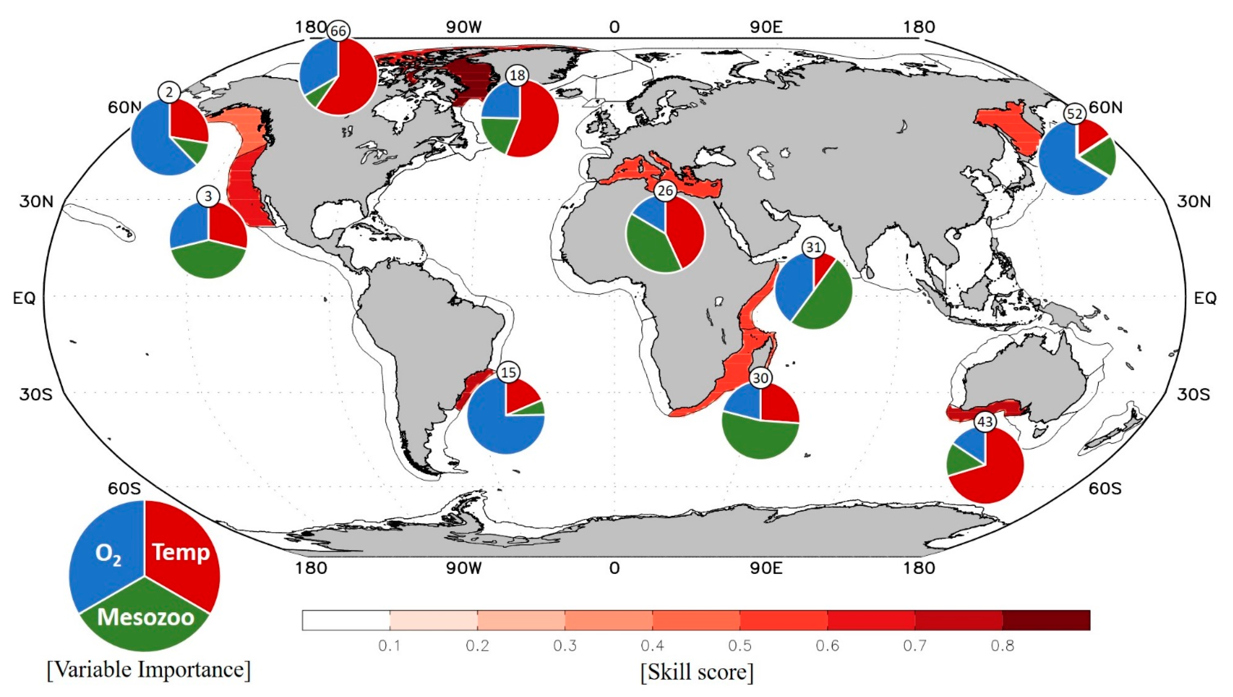
The correlation analysis assumes a linear relationship between the bottom-up factors and fisheries production, which is often limited to illuminate the nonlinear relationship between the factors and to examine the relative importance of each bottom-up driver. To supplement the linear approach, a nonlinear decision tree analysis was performed for the bottom-up driven LMEs identified from the correlation analysis above. There are 10 LMEs where a pronounced nonlinear relationship between the three environmental factors and fisheries production exists (shaded areas in Figure 3): LME #2 (Gulf of Alaska), LME #3 (California Current), LME #15 (South Brazil Shelf), LME #18 (Canadian Eastern Arctic), LME #26 (Mediterranean Sea), LME #30 (Agulhas Current), LME #31 (Somali Coastal Current), LME #43 (Southwest Australian Shelf), LME #52 (Sea of Okhotsk), and LME #66 (Canadian High Arctic). In these LMEs, the skill score that measures how well the environmental drivers explain fish catch variations from the bootstrapping decision tree analysis is in the range of 0.50–0.83 (see Methods; Figure 3).
The relative importance of each bottom-up driver for fish catch obtained from the nonlinear bootstrapping analysis is generally consistent with that from the linear correlation analysis (cf. Figure 2 and Figure 3). That is, the driver exhibiting the highest correlation coefficient with fish catch shown in Figure 2 matches with the variable with the highest importance. An exception exists: for example, LME #15 (South Brazil Shelf) was temperature-driven in the correlation analysis, while oxygen-driven in the decision tree analysis, indicating a potential nonlinear dynamic of fisheries to multiple bottom-up drivers.
The dominant drivers for fish catch at some LMEs are also largely consistent with previous works, showing that the plankton food web (represented by mesozooplankton production) dominates fish catch variations in LME #3 (California Current), LME #30 (Agulhas Current), and LME #31 (Somali Coastal Current) systems [11,17], as shown in Figure 3. However, LME #2 (Gulf of Alaska) was previously known as a temperature-driven region, while both linear and nonlinear analysis conducted here shows that oxygen better explains fish catch variations in this region than temperature. This may imply that the nonlinear analysis with the inclusion of oxygen further illuminates the relative dominance of different factors and also better isolates bottom-up driven signals in a certain LME.
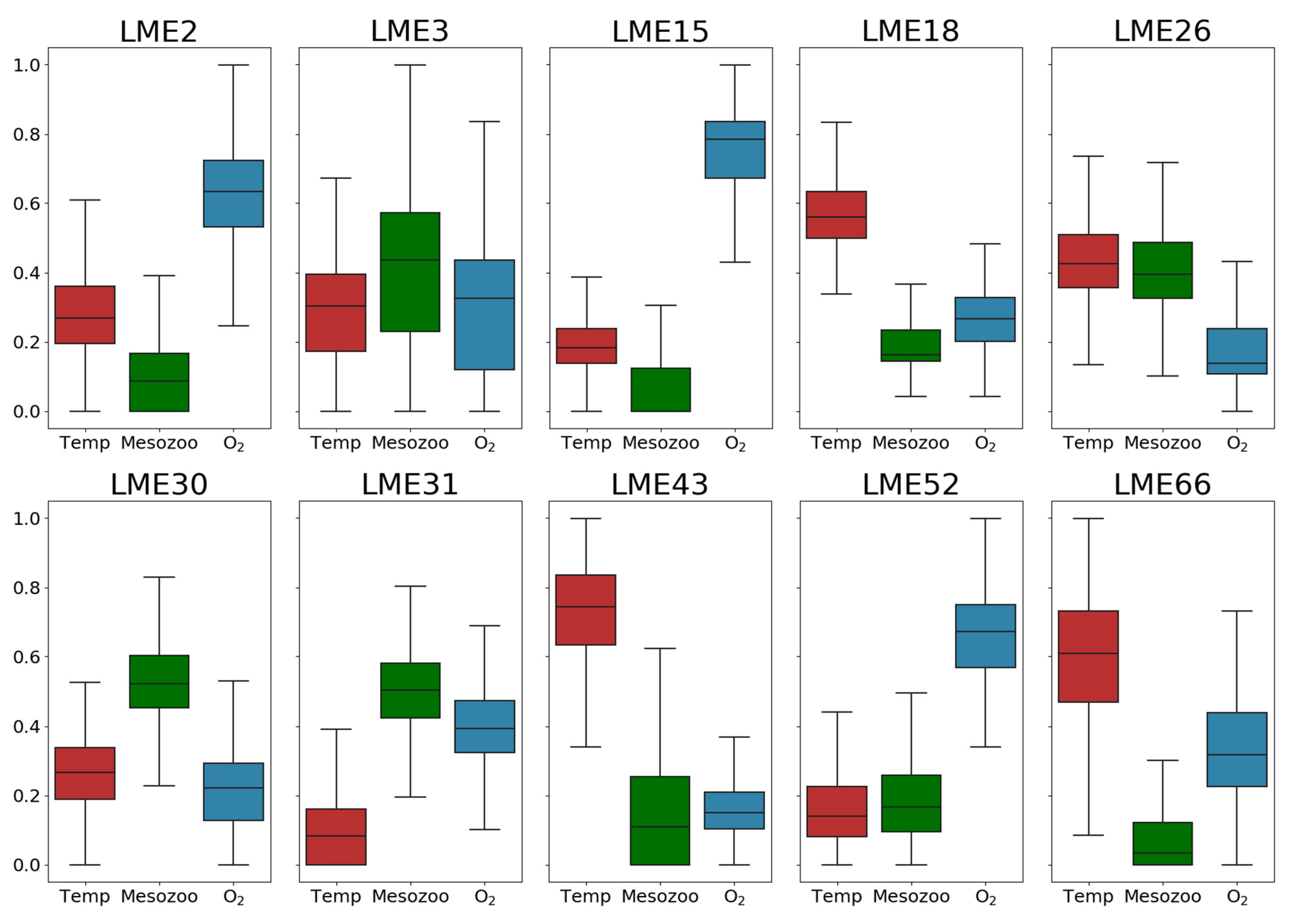
Although 7 out of 10 environmentally driven LMEs feature a single dominant driver for fish catch, the most dominant driver is not significantly separated from other drivers in LME #3 (California Current), LME #26 (Mediterranean Sea), and LME #31 (Somali Coastal Current), as shown in the probability distribution of variable importance (Figure 4). Previously, plankton production was known to be the key factor for fish catch in LME #3, the California Current system [11], but temperature and oxygen also turned out to be important drivers from the current analysis. Similarly, fish catch in LME #31, Somali Coastal Current, is dominated by two factors, plankton production and oxygen, although this region was previously identified as a plankton production driven region. These different results are presumably attributed to the relatively short data period of satellite chlorophyll used in the previous study or possible bias in aggregated catch statistics and the influence of other factors such as fishing efforts, which are not considered in the present study [41,42].
3.3. Thresholds of Multiple Environmental Forcing for High and Low Fish Catch
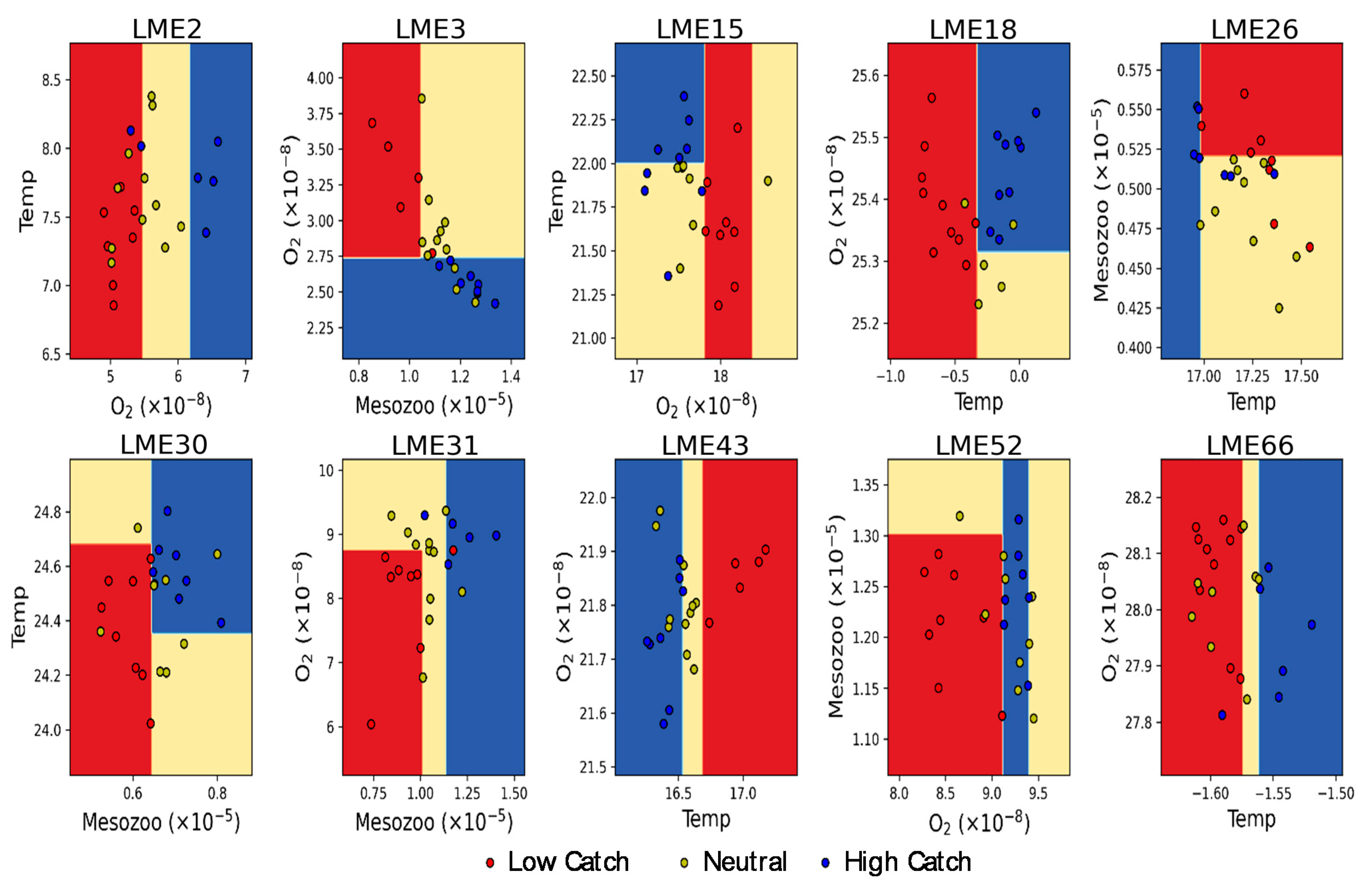
Quantitative thresholds of the three environmental factors determining high and low fish catch potentially provide guidance for marine resource management. Here, as a proof-of-concept study, a decision surface showing the boundaries of high and low fish catch is constructed by using two leading environmental drivers (Figure 5). The max depth of the tree was limited to two to avoid over fitting and to obtain straightforward thresholds for fish catch estimation. The high and low catch at each LME are well separated by conditional thresholds of multiple drivers. For example, in LME #30 (Agulhas Current) region, mesozooplankton production over 6.2 µmol m−2 s−1 and temperature over 24.35 °C provide high fish catch, while mesozooplankton production below 6.2 µmol m−2 s−1 and temperature below 24.68 °C provide low catch. The overlap in the temperature threshold for high and low catch implies nonlinear dynamics in the relationship with fisheries. In LME #3 (California Current), where all of three environmental drivers turned out to be important for fish catch estimation, the decision boundary for high catch is an oxygen level of 0.027 µmol kg−1, and that for low catch is mesozooplankton production of 12 µmol m−2 s−1 and oxygen level of 0.027 µmol kg−1. The negative relationship between oxygen concentration and fish catch may represent either the larger subsurface oxidation due to the larger surface primary production or the vertical contraction of metabolically viable habitats due to the upwelling of the oxygen minimum zone and the consequent high catch in the upper ocean layer [43].
4. Discussion
There are ten LMEs (out of 54 analyzed LMEs after excluding 12 regions due to data reliability issues) that meet the criteria for bottom-up forcing for fish catch variations, which resulted from a stringent test using both raw and detrended data. In other LME regions, fish catch variations are probably predominated by top-down drivers such as fishing effort and harvest control or are influenced by factors not considered in our study. Given that expanding fishing effort and subsequent effects of overfishing may create general trends over the time period analyzed here, LMEs where a significant relationship is evident only in the analysis with the raw (i.e., non-detrended) data may reflect top-down driven regions, which is one of the approaches used to disentangle the top-down impact on fisheries [11].
Although only a limited number of LMEs are identified in the present study, many significant relationships for individual climate-sensitive fish stocks may also underlie aggregate catch relationships. For example, pelagic and demersal species are quite different in life traits and catch variation scale, thus the similar analysis with species level can better isolate bottom-up signal in other LME regions. In fact, the bottom-up signals and the thresholds for high and low catches become much more useful when the information can be provided in a fishery- or species-dependent manner. Moreover, further applications of global-scale relationships to regional fisheries production are also possible if one uses other fish catch analysis models (e.g., Gordon–Schaefer model) [44,45]
Another limitation of the present study is that there are generally long-lag relationships in fisheries and other ecological systems given the cumulative integrations of environmental forcing and the consequent low frequency variability of large marine organisms. Previous studies already showed this in both observations and models [46,47]. Given that the significant relationship between bottom-up drivers and fish catch at longer time lags probably comes from long-lived large species, significant correspondence to individual species or functional types may be possible in other LMEs with an extended time lag correlation. Nevertheless, the main focus of the present study is to capture signals linked to contemporaneous signals for which the predictive use of them would be most useful for fisheries management and to show potential bottom-up driven linkage by using the long-term data assimilative model data.
5. Conclusions
Revisiting bottom-up forcing for fish catch with newly developed long-term reconstructed data reveals that historical fish catch variations in some large coastal areas are significantly explained by biotic and abiotic factors, including temperature, zooplankton production, and dissolved oxygen concentration, all of which are based on physiology and trophodynamics of marine biology. With the aid of a nonlinear and multivariate machine learning analysis and the inclusion of reconstructed oxygen and zooplankton production data, this study provides richer information on the potential relationship between bottom-up drivers and fisheries production across globally distributed ecosystems. Additional coastal ecosystems are identified as being driven by oxygen, which has not been investigated before due to the lack of globally available oxygen data. Moreover, the relative importance of each driver and thresholds for high and low fish catch can provide further insight into mechanistic principles of fish catch in individual coastal ecosystems.
Despite the complexity of marine ecological systems that is not fully considered in the present study, the results presented herein suggest the mechanistically consistent linkage between bottom-up forcing and fish catch and can be utilized to facilitate the ecosystem-based fisheries management strategies in a changing climate. Moreover, given that the most critical assessment in our study is the capacity of the data from the assimilative models to connect with fish catches across different global ecosystems, the result shown here provides a meaningful global assessment that will spur further refinements of research methods.
Author Contributions
J.-Y.P. and H.-J.S. contributed equally to conceptualizing the study and discussing the results. H.-J.S. led data analyzing work, and J.-Y.P. contributed substantially to writing the manuscript. All authors have read and agreed to the published version of the manuscript.
Funding
This research was funded by the National University Promotion Program in 2019 and by the National Research Foundation of Korea (NRF-2020R1C1C1008631). J.-Y.P. was supported by NOAA’s marine ecosystem tipping points initiative. H.-J.S. was supported by the National Research Foundation of Korea (NRF) grant funded by the Korea government (MSIT) (No. 2020R1F1A1072315).
Acknowledgments
The authors acknowledge the fish catch data provided by the Sea Around Us Project (http://www.seaaroundus.org).
Conflicts of Interest
The authors declare no conflict of interest.
References
- Ottersen, G.; Kim, S.; Huse, G.; Polovina, J.J.; Stenseth, N.C. Major Pathways by which Climate may Force Marine Fish Populations. J. Mar. Syst. 2010, 79, 343–360. [Google Scholar] [CrossRef]
- Finney, B.P.; Alheit, J.; Emeis, K.-C.; Field, D.B.; Gutiérrez, D.; Struck, U. Paleoecological Studies on Variability in Marine Fish Populations: A Long-Term Perspective on the Impacts of Climatic Change on Marine Ecosystems. J. Mar. Syst. 2010, 79, 316–326. [Google Scholar] [CrossRef]
- Deutsch, C.; Ferrel, A.; Seibel, B.; Pörtner, H.-O.; Huey, R.B. Climate Change Tightens a Metabolic Constraint on Marine Habitats. Science 2015, 348, 1132–1135. [Google Scholar] [CrossRef] [Green Version]
- Bopp, L.; Resplandy, L.; Orr, J.C.; Doney, S.C.; Dunne, J.P.; Gehlen, M.; Halloran, P.R.; Heinze, C.; Ilyina, T.; Seferian, R.; et al. Multiple Stressors of Ocean Ecosystems in the 21st Century: Projections with CMIP5 Models. Biogeosciences 2013, 10, 6225–6245. [Google Scholar] [CrossRef] [Green Version]
- Perry, A.L.; Low, P.J.; Ellis, J.R.; Reynolds, J.D. Climate Change and Distribution Shifts in Marine Fishes. Science 2005, 308, 1912–1915. [Google Scholar] [CrossRef]
- Doney, S.C.; Ruckelshaus, M.; Duffy, J.E.; Barry, J.P.; Chan, F.; English, C.A.; Galindo, H.M.; Grebmeier, J.M.; Hollowed, A.B.; Knowlton, N.; et al. Climate Change Impacts on Marine Ecosystems. Annu. Rev. Mar. Sci. 2012, 4, 11–37. [Google Scholar] [CrossRef] [Green Version]
- Cheung, W.W.L.; Sarmiento, J.L.; Dunne, J.P.; Frölicher, T.L.; Lam, V.W.Y.; Palomares, M.L.D.; Watson, R.; Pauly, D. Shrinking of Fishes Exacerbates Impacts of Global Ocean Changes on Marine Ecosystems. Nat. Clim. Chang. 2013, 3, 254–258. [Google Scholar] [CrossRef]
- Hare, J.A.; Alexander, M.A.; Fogarty, M.J.; Williams, E.H.; Scott, J.D. Forecasting the Dynamics of a Coastal Fishery Species using a Coupled Climate–Population Model. Ecol. Appl. 2010, 20, 452–464. [Google Scholar] [CrossRef]
- Essington, T.E.; Moriarty, P.E.; Froehlich, H.E.; Hodgson, E.E.; Koehn, L.E.; Oken, K.L.; Siple, M.C.; Stawitz, C.C. Fishing Amplifies Forage Fish Population Collapses. Proc. Natl. Acad. Sci. USA 2015, 112, 6648–6652. [Google Scholar] [CrossRef] [PubMed] [Green Version]
- Sharp, G.D. Climate and Fisheries: Cause and Effect or Managing the Long and Short of it All. S. Afr. J. Mar. Sci. 1987, 5, 811–838. [Google Scholar] [CrossRef]
- McOwen, C.J.; Cheung, W.W.L.; Rykaczewski, R.R.; Watson, A.R.; Wood, L.J. Is Fisheries Production within Large Marine Ecosystems Determined by Bottom-Up or Top-Down Forcing? Fish Fish. 2014, 16, 623–632. [Google Scholar] [CrossRef]
- Stock, C.A.; John, J.G.; Rykaczewski, R.R.; Asch, R.G.; Cheung, W.W.L.; Dunne, J.P.; Friedland, K.D.; Lam, V.W.Y.; Sarmiento, J.L.; Watson, R.A. Reconciling Fisheries Catch and Ocean Productivity. Proc. Natl. Acad. Sci. USA 2017, 114, E1441–E1449. [Google Scholar] [CrossRef] [Green Version]
- Nieto, K.; McClatchie, S.; Weber, E.D.; Lennert-Cody, C.E. Effect of Mesoscale Eddies and Streamers on Sardine Spawning Habitat and Recruitment Success off Southern and Central California. J. Geophys. Res. Oceans 2014, 119, 6330–6339. [Google Scholar] [CrossRef]
- Tommasi, D.; Stock, C.A.; Pegion, K.; Vecchi, G.A.; Methot, R.D.; Alexander, M.A.; Checkley, D.M. Improved Management of Small Pelagic Fisheries through Seasonal Climate Prediction. Ecol. Appl. 2017, 27, 378–388. [Google Scholar] [CrossRef] [PubMed]
- Lindegren, M.; Checkley, D.M. Temperature Dependence of Pacific Sardine (Sardinops Sagax) Recruitment in the California Current Ecosystem Revisited and Revised. Can. J. Fish. Aquat. Sci. 2013, 70, 245–252. [Google Scholar] [CrossRef] [Green Version]
- Fu, C.; Gaichas, S.; Link, J.S.; Bundy, A.; Boldt, J.L.; Cook, A.M.; Gamble, R.; Utne, K.R.; Liu, H.; Friedland, K.D. Relative Importance of Fisheries, Trophodynamic and Environmental Drivers in a Series of Marine Ecosystems. Mar. Ecol. Prog. Ser. 2012, 459, 169–184. [Google Scholar] [CrossRef] [Green Version]
- Park, J.-Y.; Stock, C.A.; Dunne, J.P.; Yang, X.; Rosati, A. Seasonal to Multiannual Marine Ecosystem Prediction with a Global Earth System Model. Science 2019, 365, 284–288. [Google Scholar] [CrossRef]
- Sachoemar, S. Variability of Sea Surface Chlorophyll-A, Temperature and Fish Catch within Indonesian Region Revealed by Satellite Data. Mar. Res. Indones. 2012, 37, 75–87. [Google Scholar] [CrossRef]
- Solanki, H.U.; Dwivedi, R.M.; Nayak, S.R. Synergistic Analysis of SeaWiFS Chlorophyll Concentration and NOAA-AVHRR SST Features for Exploring Marine Living Resources. Int. J. Remote Sens. 2001, 22, 3877–3882. [Google Scholar] [CrossRef]
- Antoine, D.; Morel, A.; Gordon, H.R.; Banzon, V.F.; Evans, R.H. Bridging Ocean Color Observations of the 1980s and 2000s in Search of Long-Term Trends. J. Geophys. Res. Space Phys. 2005, 110, 110. [Google Scholar] [CrossRef]
- Friedland, K.D.; Stock, C.; Drinkwater, K.F.; Link, J.S.; Leaf, R.T.; Shank, B.V.; Rose, J.M.; Pilskaln, C.H.; Fogarty, M.J. Pathways between Primary Production and Fisheries Yields of Large Marine Ecosystems. PLoS ONE 2012, 7, e28945. [Google Scholar] [CrossRef] [PubMed] [Green Version]
- Park, J.-Y.; Stock, C.A.; Yang, X.; Dunne, J.P.; Rosati, A.; John, J.; Zhang, S. Modeling Global Ocean Biogeochemistry With Physical Data Assimilation: A Pragmatic Solution to the Equatorial Instability. J. Adv. Model. Earth Syst. 2018, 10, 891–906. [Google Scholar] [CrossRef]
- Zhang, S.; Harrison, M.J.; Rosati, A.; Wittenberg, A. System Design and Evaluation of Coupled Ensemble Data Assimilation for Global Oceanic Climate Studies. Mon. Weather Rev. 2007, 135, 3541–3564. [Google Scholar] [CrossRef] [Green Version]
- Kanamitsu, M.; Ebisuzaki, W.; Woollen, J.; Yang, S.-K.; Hnilo, J.J.; Fiorino, M.; Potter, G.L. NCEP–DOE AMIP-II Reanalysis (R-2). Bull. Am. Meteorol. Soc. 2002, 83, 1631–1644. [Google Scholar] [CrossRef]
- Levitus, S.; Antonov, J.I.; Baranova, O.K.; Boyer, T.P.; Coleman, C.L.; Garcia, H.E.; Grodsky, A.I.; Johnson, D.R.; Locarnini, R.A.; Mishonov, A.V.; et al. The World Ocean Database. Data Sci. J. 2013, 12, WDS229–WDS234. [Google Scholar] [CrossRef] [Green Version]
- Reynolds, R.W.; Smith, T.M.; Liu, C.Y.; Chelton, D.B.; Casey, K.S.; Schlax, M.G. Daily High-Resolution-Blended Analyses for Sea Surface Temperature. J. Clim. 2007, 20, 5473–5496. [Google Scholar] [CrossRef]
- Roemmich, D.; Riser, S.; Davis, R.; Desaubies, Y. Autonomous Profiling Floats: Workhorse for Broad-Scale Ocean Observations. Mar. Technol. Soc. J. 2004, 38, 21–29. [Google Scholar] [CrossRef] [Green Version]
- Stock, C.A.; Dunne, J.P.; John, J.G. Global-Scale Carbon and Energy Flows through the Marine Planktonic Food Web: An Analysis with a Coupled Physical–Biological Model. Prog. Oceanogr. 2014, 120, 1–28. [Google Scholar] [CrossRef]
- Laufkötter, C.; Vogt, M.; Gruber, N.; Aita-Noguchi, M.; Aumont, O.; Bopp, L.; Buitenhuis, E.; Doney, S.C.; Dunne, J.; Hashioka, T.; et al. Drivers and Uncertainties of Future Global Marine Primary Production in Marine Ecosystem Models. Biogeosciences 2015, 12, 6955–6984. [Google Scholar] [CrossRef] [Green Version]
- Dunne, J.P.; John, J.G.; Shevliakova, E.; Stouffer, R.J.; Krasting, J.P.; Malyshev, S.L.; Milly, P.C.D.; Sentman, L.T.; Adcroft, A.J.; Cooke, W.; et al. GFDL’s ESM2 Global Coupled Climate–Carbon Earth System Models. Part II: Carbon System Formulation and Baseline Simulation Characteristics. J. Clim. 2013, 26, 2247–2267. [Google Scholar] [CrossRef] [Green Version]
- Esaias, W.; Abbott, M.; Barton, I.; Brown, O.; Campbell, J.; Carder, K.; Clark, D.; Evans, R.; Hoge, F.; Gordon, H.; et al. An Overview of MODIS Capabilities for Ocean Science Observations. IEEE Trans. Geosci. Remote Sens. 1998, 36, 1250–1265. [Google Scholar] [CrossRef] [Green Version]
- McClain, C.R.; Cleave, M.L.; Feldman, G.C.; Gregg, W.W.; Hooker, S.B.; Kuring, N. Science Quality SeaWiFS Data for Global Biosphere Research. Sea Technol. 1998, 39, 10–16. [Google Scholar]
- Pauly, D.; Zeller, D. Catch Reconstructions Reveal that Global Marine Fisheries Catches are Higher than Reported and Declining. Nat. Commun. 2016, 7, 10244. [Google Scholar] [CrossRef]
- Sherman, K. The Large Marine Ecosystem Approach for Assessment and Management of Ocean Coastal Waters. In Sustaining Large Marine Ecosystems: The Human Dimension; Hennessey, T.M., Sutinen, J.G., Eds.; Elsevier: Amsterdam, The Netherlands, 2005; Volume 13, pp. 3–16. [Google Scholar]
- Chassot, E.; Bonhommeau, S.; Dulvy, N.K.; Mélin, F.; Watson, R.; Gascuel, D.; Le Pape, O. Global Marine Primary Production Constrains Fisheries Catches. Ecol. Lett. 2010, 13, 495–505. [Google Scholar] [CrossRef]
- Bretherton, C.S.; Widmann, M.; Dymnikov, V.P.; Wallace, J.M.; Blade, I. The Effective Number of Spatial Degrees of Freedom of a Time-Varying Field. J. Clim. 1999, 12, 1990–2009. [Google Scholar] [CrossRef]
- Breiman, L.; Friedman, J.H.; Olshen, R.A.; Stone, C.J. Classification and Regression Trees; CRC Press: Boca Raton, FL, USA, 2017. [Google Scholar]
- Hastie, T.; Tibshirani, R.; Friedman, J. The Elements of Statistical Learning: Data Mining, Inference, and Prediction; Springer: Berlin/Heidelberg, Germany, 2009. [Google Scholar]
- McGovern, A.; Elmore, K.L.; Gagne, D.J.; Haupt, S.E.; Karstens, C.D.; Lagerquist, R.; Smith, T.; Williams, J.K. Using Artificial Intelligence to Improve Real-Time Decision-Making for High-Impact Weather. Bull. Am. Meteorol. Soc. 2017, 98, 2073–2090. [Google Scholar] [CrossRef]
- Chavez, F.P.; Ryan, J.; Lluch-Cota, S.E.; Ñiquen, M. From Anchovies to Sardines and Back: Multidecadal Change in the Pacific Ocean. Science 2003, 299, 217–221. [Google Scholar] [CrossRef] [Green Version]
- Chassot, E.; Melin, F.; Le Pape, O.; Gascuel, D. Bottom-Up Control Regulates Fisheries Production at the Scale of Eco-Regions in European Seas. Mar. Ecol. Prog. Ser. 2007, 343, 45–55. [Google Scholar] [CrossRef] [Green Version]
- Field, J.C.; MacCall, A.D.; Bradley, R.W.; Sydeman, W.J. Estimating the Impacts of Fishing on Dependent Predators: A Case Study in the California Current. Ecol. Appl. 2010, 20, 2223–2236. [Google Scholar] [CrossRef]
- Stramma, L.; Prince, E.D.; Schmidtko, S.; Luo, J.; Hoolihan, J.P.; Visbeck, M.; Wallace, D.W.R.; Brandt, P.; Körtzinger, A. Expansion of Oxygen Minimum Zones may Reduce Available Habitat for Tropical Pelagic Fishes. Nat. Clim. Chang. 2011, 2, 33–37. [Google Scholar] [CrossRef] [Green Version]
- Grønbæk, L.; Lindroos, M.; Munro, G.; Pintassilgo, P. Game Theory and Fisheries. Fish. Res. 2018, 203, 1–5. [Google Scholar] [CrossRef] [Green Version]
- Memarzadeh, M.; Britten, G.L.; Worm, B.; Boettiger, C. Rebuilding Global Fisheries under Uncertainty. Proc. Natl. Acad. Sci. USA 2019, 116, 15985–15990. [Google Scholar] [CrossRef] [PubMed] [Green Version]
- Di Lorenzo, E.; Ohman, M.D. A Double-Integration Hypothesis to Explain Ocean Ecosystem Response to Climate Forcing. Proc. Natl. Acad. Sci. USA 2013, 110, 2496–2499. [Google Scholar] [CrossRef] [PubMed] [Green Version]
- Le Mézo, P.; Lefort, S.; Séférian, R.; Aumont, O.; Maury, O.; Murtugudde, R.; Bopp, L. Natural Variability of Marine Ecosystems Inferred from a Coupled Climate to Ecosystem Simulation. J. Mar. Syst. 2016, 153, 55–66. [Google Scholar] [CrossRef]
Figure 1.
(Left panel from the top to the bottom) Observed annual mean surface nitrate, subsurface oxygen averaged in 200–500 m depth, and surface chlorophyll. (Right panel) Similar to left panel but for the simulated biogeochemical variables from the data assimilation run integrated with an ocean biogeochemical model.

Figure 2.
Correlation coefficients between reported annual fish catch and reconstructed environmental drivers in large marine ecosystems (LMEs) during 1991–2014. The correlation analysis is repeated with both raw (upper panel) and detrended (lower panel) data. The environmental drivers used here are annual means of ocean temperature averaged in the upper 100 m (red bars), mesozooplankton production integrated in the upper 200 m (green marks), and dissolved oxygen concentration averaged between 200 and 500 m depth (blue marks). Filled marks and bars represent significant (p < 0.10) correlation coefficients.

Figure 3.
Shaded regions represent LMEs where past fish catch variations are explained by three environmental factors: temperature, mesozooplankton production, and dissolved oxygen. Skill scores, defined from a bootstrapping decision tree method, are represented by the density of shading for each LME. Pie charts indicate the relative importance of environmental factors for historical fish catch variations in the 10 LMEs in which environmental forcing proved to be of considerable importance for fisheries (LME #2: Gulf of Alaska, LME #3: California Current, LME #15: South Brazil Shelf, LME #18: Canadian Eastern Arctic, LME #26: Mediterranean Sea, LME #30: Agulhas Current, LME #31: Somali Coastal Current, LME #43: Southwest Australian Shelf, LME #52: Sea of Okhotsk, and LME #66: Canadian High Arctic LMEs).

Figure 4.
The box-and-whisker plot of the importance of 3 environmental drivers for fish catch variation in the previously identified 10 LME regions. The importance of each variable and its uncertainty range are obtained by the statistics of 1000 importance values for each variable from the bootstrapping decision tree analysis.

Figure 5.
Decision-tree surface to show how high and low fish catches are classified at each LME region. Two leading drivers at each region are used in this analysis. The depth of the decision tree is fixed to 2 to provide a pragmatic view of potential application for fisheries management. The units for temperature, mesozooplankton production, and dissolved oxygen are °C, mol m−2 s−1, and mol kg−1, respectively.


Table 1.
The Large Marine Ecosystem (LME) name corresponding to each LME number.
| LME Number | LME Name | LME Number | LME Name | LME Number | LME Name | LME Number | LME Name |
|---|---|---|---|---|---|---|---|
| 1 | East Bering Sea | 18 | Canadian Eastern Arctic | 35 | Gulf of Thailand | 52 | Sea of Okhotsk |
| 2 | Gulf of Alaska | 19 | East Greenland Shelf | 36 | South China Sea | 53 | West Bering Sea |
| 3 | California Current | 20 | Barents Sea | 37 | Sulu-Celebes Sea | 54 | Chukchi Sea |
| 4 | Gulf of California | 21 | Norwegian Shelf | 38 | Indonesian Sea | 55 | Beaufort Sea |
| 5 | Gulf of Mexico | 22 | North Sea | 39 | North Australian Shelf | 56 | East Siberian Sea |
| 6 | Southeast U.S. Continental Shelf | 23 | Baltic Sea | 40 | Northeast Australian Shelf | 57 | Laptev Sea |
| 7 | Northeast U.S. Continental Shelf | 24 | Celtic-Biscay Shelf | 41 | East-Central Australian Shelf | 58 | Kara Sea |
| 8 | Scotian Shelf | 25 | Iberian Coastal | 42 | Southeast Australian Shelf | 59 | Iceland Shelf |
| 9 | Newfoundland-Labrador Shelf | 26 | Mediterranean Sea | 43 | Southwest Australian Shelf | 60 | Faroe Plateau |
| 10 | Insular Pacific-Hawaiian | 27 | Canary Current | 44 | West-Central Australian Shelf | 61 | Antarctica |
| 11 | Pacific Central-American | 28 | Guinea Current | 45 | Northwest Australian Shelf | 62 | Black Sea |
| 12 | Caribbean Sea | 29 | Benguela Current | 46 | New Zealand Shelf | 63 | Hudson Bay |
| 13 | Humboldt Current | 30 | Agulhas Current | 47 | East China Sea | 64 | Arctic Ocean |
| 14 | Patagonian Shelf | 31 | Somali Coastal Current | 48 | Yellow Sea | 65 | Aleutian Islands |
| 15 | South Brazil Shelf | 32 | Arabian Sea | 49 | Kuroshio Current | 66 | Canadian High Arctic |
| 16 | East Brazil Shelf | 33 | Red Sea | 50 | East Sea | ||
| 17 | North Brazil Shelf | 34 | Bay of Bengal | 51 | Oyashio Current |
Publisher’s Note: MDPI stays neutral with regard to jurisdictional claims in published maps and institutional affiliations. |
© 2021 by the authors. Licensee MDPI, Basel, Switzerland. This article is an open access article distributed under the terms and conditions of the Creative Commons Attribution (CC BY) license (https://creativecommons.org/licenses/by/4.0/).
Share and Cite
MDPI and ACS Style
Song, H.-J.; Park, J.-Y. Bottom-Up Drivers for Global Fish Catch Assessed with Reconstructed Ocean Biogeochemistry from an Earth System Model. Climate 2021, 9, 83. https://0-doi-org.brum.beds.ac.uk/10.3390/cli9050083
AMA Style
Song H-J, Park J-Y. Bottom-Up Drivers for Global Fish Catch Assessed with Reconstructed Ocean Biogeochemistry from an Earth System Model. Climate. 2021; 9(5):83. https://0-doi-org.brum.beds.ac.uk/10.3390/cli9050083
Chicago/Turabian StyleSong, Hyo-Jong, and Jong-Yeon Park. 2021. "Bottom-Up Drivers for Global Fish Catch Assessed with Reconstructed Ocean Biogeochemistry from an Earth System Model" Climate 9, no. 5: 83. https://0-doi-org.brum.beds.ac.uk/10.3390/cli9050083
Note that from the first issue of 2016, this journal uses article numbers instead of page numbers. See further details here.