
Costs and Distributional Effects of Climate Transformation of the Vehicle Fleet in the EU

1
Department of Economics, Swedish University of Agricultural Sciences, 75007 Uppsala, Sweden
2
School of Social Science, Södertörn University, 14189 Huddinge, Sweden
*
Author to whom correspondence should be addressed.
Climate 2021, 9(6), 88; https://0-doi-org.brum.beds.ac.uk/10.3390/cli9060088
Submission received: 12 April 2021
/
Revised: 16 May 2021
/
Accepted: 19 May 2021
/
Published: 21 May 2021
(This article belongs to the Special Issue Anthropogenic Climate Change: Social Science Perspectives)
Abstract
:This study estimates the minimum total cost and distributional effects among countries transforming the car fleet in the EU to reduce emissions of carbon dioxides by 2050 by switching from fossil fuel-driven passenger cars to hybrid and electric-driven cars. Minimum cost is estimated using a dynamic optimization model in which costs are calculated as decreases in consumer surplus in the demand for vehicles under given annual increases in travel demand, carbon efficiency and technological improvement of electric cars. Distributional effects are calculated for the cost-effective allocation of costs among the EU member states and UK. Calculations are made for different emission reductions, and the cost for achieving a 60% reduction from the 1990 emission level ranges between 0.13% and 0.61% of the EU’s GDP depending on assumptions about development of travel demand and carbon efficiency. The results indicate a slightly regressive allocation in most scenarios, where the cost share is relatively high for low income countries.
1. Introduction
The transport sector accounts for approximately 25% of the total greenhouse gas (GHG) emissions in the EU in 2018 [1] and light duty vehicles account for about 45% of the emissions from transport sector [2]. In order to reduce CO2 emissions from the transport sector, the EU has outlined a 20% reduction in emission below the 2008 level by 2030, and of at least 60% by 2050 compared to the 1990 levels and have introduced emission standards for new cars and vans [3]. As shown in several studies, demand for transports by car are likely to increase because of increase in income and wealth in many EU countries (e.g., [4]).
For unchanged or increasing demand for transport by cars, climate transformation, which is defined as reductions in CO2 emissions, can be made by increasing fuel efficiency in cars that run on fossil fuels, by switching from fossil fuel engines to hybrid and electric cars, and by changing transport mode to, e.g., train and public transports. The widely used types of passenger vehicles are gasoline and diesel-powered vehicles that emit more kg CO2/km travelled than emissions from hybrid and electric vehicles. Several studies have shown that the emission reduction potential of changed transport mode and carbon efficiency increase by fossil fuel cars is limited, which requires large transformation to hybrid and electric cars to reach considerable climate targets in 2050 (e.g., [5]). The share of hybrid and electric passenger cars is approximately 2% and 0.15% in Europe respectively in 2018 [6], and the predicted shares in 2050 are not sufficient for large emission reductions [4].
The EU policy for reducing emissions from transports and other sectors are guided by concern of cost-effectiveness and fairness in distributional effects [3]. Cost-effectiveness of different measures and policies has been examined in several studies, but in different ways. One is by calculating and comparing cost per unit emission reduction for different measures, such as speed reduction or cost of switching from fossil fuel to electric vehicle (see Kok et al. [7] for a review). These studies do not provide information on total costs for given emission reductions or allocation of costs among different groups. Minimum total cost for emission reductions has been calculated by studies using numerical partial equilibrium models at the regional or global scale that simulate the costs of climate targets for the transport and energy sectors (see review in Bosetti and Longden [8]). These studies show that hybrid and electric light-duty vehicles have the potential to decrease emissions and reduce the cost of achieving emission targets.
Concern about distributional effects of transport policies is revealed by policy making in practice, e.g., the EU criteria for effort sharing schemes in the 2030 targets [3]. It has been shown in the literature that regressive income distributional effects (i.e., proportionally large welfare loss for low income actors) of climate and other policies influence the acceptance and thereby the implementation of climate and environmental policies (e.g., [9,10]). Several studies have defined and measured distributional effects of carbon policies on fuel (see review in Sterner [11]). A common result is that transport fuel polices can be costly and regressive, i.e., that relatively low income groups pay proportionally large shares of the policy cost. Regressive incidences are likely to impede implementation and enforcement of policies in general, which has been demonstrated by citizens’ protests against increased fuel taxes in, e.g., France and Sweden.
The purpose of this study is twofold, to calculate cost-effective solutions to different emission reductions from passenger cars in the EU and UK by 2050 and to assess distributional effects of the cost allocations on the EU member states and the UK. To this end, we apply an alternative approach compared with the studies on unit costs and policy analysis where a dynamic optimization model is developed to minimize costs for future emissions reductions from passenger cars by changes in the allocation of vehicles. Similar dynamic optimization models have been applied to other sectors, such as cost-effective provision of carbon sequestration by forests (e.g., [12,13]). The numeral model accounts for annual exogenous chances in travel demand, carbon efficiency and prices of new vehicles. Distributional effects of the cost-effective allocation of cost among countries are measured in two ways. One is the calculation of the Suits index, which shows the existence and magnitude of regressive or progressive outcomes and is much used in the literature (e.g., [11,14,15]). The other is a ranking of cost burdens in relation to a country’s total income, which indicates whether the shares are proportionally high for low income countries.
In our view, the contribution of the present study is the calculation of minimum cost solutions for CO2 reductions from passenger cars in the EU and UK with a dynamic optimization model and assessment of distributional effects. To the best of the author’s knowledge there has been no study using dynamic optimization to calculate the minimum costs of achieving the EU’s 2050 emission reductions for the transport sector. The studies on unit cost estimates of different vehicles do not calculate minimum costs for given emission reductions [7]. The spatial division of the models calculating minimum costs is on large country levels and an aggregation of small countries, and they do not generate information on costs for countries within the EU. Further, they do not allow for the cost-effective allocation of vehicles and other measures over time and have not been used to assess distributional effects of cost allocations. Costs and distributional effects have been assessed by simulations of models of transport demand systems in different EU countries, but without calculations of cost-effective solutions for achievement of common emission reduction targets (e.g., [11,16]). Minimum costs and distributional effects of reductions in emissions from transport fuel have been calculated for single countries (e.g., [15]), but not in a dynamic perspective.
Simplifications are made by using the marginal abatement cost approach, which is applied in several other studies (e.g., [17,18]). This approach considers only costs for the sectors or actors directly affected by the emission reduction, such as decreases in profits from reduction in the use of fossil fuel in the industry and energy producing sectors. In the present study, car owners are directly affected by the switch from fossil fuel cars to cars with lower emissions. Costs are then calculated as associated decreases in the car owners’ welfare, which is measured by decreases in consumer surplus. The advantage of the simplicity in the cost measurement is that it allows for a dynamic optimization, which accounts for changes in travel demand, carbon efficiency and vehicle prices over time.
The study is organized as follows. Section 2 develops the dynamic optimization model underlying the calculations, with the data described in Section 3. Scenarios regarding assumptions on future development of travel demand and carbon efficiency for costs are minimized are described in Section 4, and the results are presented in Section 5. The model and results are discussed in Section 6, which also contains concluding remarks.
2. Conceptual Approach
The analysis consists of two main parts; minimization of cost for achieving given emission reductions and assessment of associated distributional effects among the countries. The structure of the dynamic optimization model is described in this section together with the chosen measurements of distributional effects. Unless otherwise stated, all proofs are found in Appendix A.
2.1. Dynamic Optimization Model
The minimum cost of CO2 reduction in emissions from light-duty vehicles by changing the allocation of carbon intensive vehicles is calculated within a discrete time non-linear dynamic programming model. The change is made from fossil fuel vehicles, F, that run on either gasoline or diesel to hybrid, H, and electric, E, vehicles. There are a variety of hybrid vehicles that utilize more than one form of energy. The most widely used are hybrid gasoline and hybrid diesel that run on a combination of fossil fuel and electricity. They mostly derive electricity either through an internal generation system, such as regenerative braking, or through a plug-in charging system. Other types that could be considered hybrid include semi-biofuel-driven vehicles. A simplification in this study is that all these varieties of hybrid cars, defined as vehicles that run on a mix of fossil fuel and more than 5% biofuel, semi-electric and semi-biofuel or semi-fossil fuel are classified as hybrid vehicles. Electric vehicles are defined as battery-powered fully electric-driven vehicles. Vehicles that run solely on electricity have zero exhaust emissions, but emission is dependent on the source of electricity.
The stock of vehicles in each country , in the EU and UK for vehicle type , at time is determined by a constant depreciation rate , which differs among the countries and vehicle types, and the purchase of new vehicles , which is written as:
where for .
The demand for travel , is exogenous to the model and measured in the number of kilometers traveled. The demand is expected to increase over time at different rates in the EU countries and UK (EC, 2016), which is written as a country specific constant annual rate of increase, . It is assumed that the travel intensity measured as kilometers travelled per vehicle, fi, differs among countries but is the same for vehicle types, i.e., . The restriction on the travel demand for each country and time period is then written as:
Emissions of CO2 from travel in each country and period of time is measured as the product of consumption of fuel type per kilometer , kilometers travelled per vehicle , and the number of vehicles per engine energy type, . A technological improvement in fuel efficiency in each country, i.e., in , is assumed where the emission per kilometer is decreasing at an annual rate of , where . This assumption is in line with the observed fuel efficiency increase of passenger cars in the EU in the last few decades [19]. A simplification is made by assuming exogenous increases in fuel efficiency. This is in contrast to the relatively large body of literature on endogenous development of the transport vehicles technology development occurs as a response to, among other things, investment, demand generated by income growth and environmental regulatory pressures (e.g., [20,21]), learning by research (e.g., [8]) and learning by doing (e.g., [22]). The justification for this simplification is the calculation of costs only for car owners in different EU countries to reach the CO2 emission targets, which are assumed to perceive technological development as given. Total emission at time t, , is then the sum of emission from the stock of vehicle type in EU-27 member states (MS) and UK:
where shows the emission per km in period t at the annual rate of carbon efficiency αj by vehicle type j from period 0.
Within the EU, there are no targets for reductions in emissions specifically from light-duty vehicles but only from the transport sector by 2050. Therefore, successive changes in emission targets, , where T is the target year 2050, are made in order to derive an EU-UK cost function for 2050. The emission constraint is written as:
The cost of reducing emission from fossil fuel vehicles through changes in the allocation of vehicles is denoted , which is calculated as decreases in consumer surplus from the demand of in the business-as-usual case. By assumption, the prices in the BAU show consumers willingness to pay for each car type, which includes perceived costs of driving the car, depreciation, etc. The cost from deviation from these prices and quantities then reflects consumer losses from paying a higher price than willingness to pay for hybrid and electric cars and from lost values in excess of the price for fossil fuel cars. Changes in consumer surplus are estimated by assumption of linear demand functions, which are derived from data on price elasticities, price and demand for in the reference year . It is then assumed that the prices are given and that the demand function in each country and for each vehicle type shifts according to changes in travel demand in the business as usual.
The costs of new cars may change over time because of, among other things, the fall in the price of electric cars due to improved batteries. Similar to technological change in fuel efficiency, we assign an exogenous and monotonic change in costs, which is written as:
where is the annual rate of change in the costs of passenger car. The cost function is assumed to be continuous, decreasing and convex in its arguments. This is to ensure that the second-order conditions of minimization are satisfied.
The decision problem is formulated as minimizing total cost in present terms, TC, under restriction on travel demand and maximum emission, Equations (3) and (4) respectively, which is written as:
Subject to Equations (1)–(5), where is the discount factor with the social discount rate , which is assumed to be the same for all countries. The properties of the cost-effective solution are derived from the first-order condition:
where . The parameter denotes the marginal cost of achieving the emission target in year 2050, and is the marginal cost of travel demand in each country and time period. According to Equation (7), a cost-effective solution requires that marginal cost of an emission reduction in the target year is equal for all countries and vehicles and amounts to θ. This implies that, ceteris paribus, car switches are targeted towards reductions in vehicles with relatively large impacts on emission reductions, i.e., large carbon emission per kilometer, as shown by the denominator at the left hand side of Equation (7). When considering optimal timing of vehicle changes there are two counter acting forces. The discount factor and the exogenous changes in carbon efficiency and prices of non-fossil fuel cars favor delays of cars shifts since the cost of and emissions from new cars decrease over time. On the other hand, the increasing travel demand over time requires sufficiently early switches in order to obtain the emission constraint, shown by the second term within brackets on the left hand side of Equation (7).
2.2. Distributional Effects
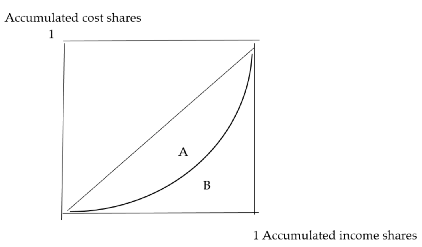
The cost-effective solutions will give rise to allocation of costs among countries, the effects of which can be of concern for policy makers. For example, the allocation of emission reductions in the effort sharing scheme for meeting the 2030 EU climate target accounts for fairness [23]. The targets to be achieved are then divided among the countries according to their GDP/capita where the emission target is relatively low for low income countries, and vice versa. Several studies have shown that environmental taxation of cars and/or fuel is in general progressive although some studies show regressive effects (see review in [11]). It is common to measure existence and magnitude of regressivity/progressivity by the Suits index, which relates the proportion of accumulated costs to proportions of accumulated income for different groups [24]. The index is zero when costs are proportional to income, it is negative when low income groups face proportionally large share of total cost, and positive when the proportion of costs is relatively large for high income countries.
The calculation of the Suits index is based on the construction of Lorenz curves, which relate the accumulated emission reduction cost shares to income shares for the counties. Two different curves are illustrated in Figure 1 where the Y-axis shows accumulated increasing cost shares and the X-axis is the accumulated increasing income shares. The linear Lorenz curve shows a neutral allocation of costs when the Suits index is zero since the share of the cost burden is the same as the share of total income at all levels. The nonlinear curve illustrates a progressive allocation where low income groups pay a relatively low share of the total cost.
The Suits index was calculated as the ratio between the area A in relation to the area with a neutral allocation of costs, i.e., the area under the line that corresponds to 0.5 (i.e., area A + area B). We then had that the Suits index corresponded to Area A/0.5, which gives 1 − AreaB/0.5 since Area A = 0.5 − Area B (see e.g., [11]). In this study Area B was calculated as the sum of trapezoid areas of accumulated shares of income and costs for each country.
The Suits index may hide costs that are high in relation to income for some groups (e.g., [14]). In order to examine this, we also calculated cost in relation to prosperity, measured as income per capita, for the EU MS and UK.
3. Description of Data
In order to solve the numerical problem, data are needed on vehicles stocks and depreciation, travel demand, CO2 intensity to calculate emissions and on discount rate, car sales and prices to calculate costs in terms of reductions in consumer surplus over time. The latest necessary data on these variables are available for 2018, which then constitutes the base year. Given the EU climate targets to be achieved by 2050, this year was used as the target year for emission reductions from light-duty vehicles. Unless otherwise stated all data are found in Appendix B.
3.1. Car Fleet, Travel Demand and CO2 Emissions
The passenger car stock and number of new passenger cars were classified into fossil fuel, hybrid and electric, and data were obtained from Eurostat [6,25]. In total, there were almost 270 million passenger cars in the EU in 2018, of which 96% were fossil fuel-driven, 3.6% were hybrid and 0.2% were electric-driven passenger cars. Approximately 17 million new vehicles were registered in the same year, but with higher shares of hybrid and electric cars than for the stock, 3.8% and 0.9%, respectively.
Data on travel demand measured as kilometers driven and fuel consumption were obtained from Eurostat [6,26]. The database does not cover annual average kilometers traveled by passenger cars for all countries but are missing for approximately 40% of the EU countries and a combination of data sources have therefore been used.
Data on emissions of CO2 from passenger cars per kilometer of travel is obtained from EC [4] for fossil fuel cars (Appendix B Table A3). For electric cars, emission per travelled kilometers depends on the sources of electricity production, which differ between the EU countries. For example, a large part of the electricity production in Poland is based on coal and in Sweden on hydropower. The emission levels are obtained from Aklilu [27] who used Eurostat data of CO2 emission per kWh of gross electricity production for each EU-28 country multiplied by average electricity consumption per kilometer. The use of electricity per kilometer depends on the type of car and reports from studies range between 0.145 and 0.20 kWh/km [28]. In the present study the average of 0.173 kWh/km was used. The emission from hybrid cars depends on their operation in electric, fossil and bio fuel modes. Due to a lack of data, it is simply assumed that the emission from hybrid cars corresponds to the average of the emissions from the fuel and electricity cars in each country.
With respect to the depreciation rate of fossil fuel cars, it is calculated by the use of data on average life time of registered cars [29], which ranges from 7 (Luxemburg) to 17 years (Latvia and Estonia). The average annual depreciation rates then varied between 0.06 and 0.15. The lifespan of electric passenger cars is mainly determined by the lifespan of the battery. The commonly used battery in electric cars that is a lithium-ion battery with a lifespan ranging from 5 to 15 years [30]. The average was taken and a depreciation rate of 10% was assumed. Hybrid vehicles were assumed to have a lifespan of 13 years, which falls between fossil fuel and electric cars [31,32]. This implies that 7.69% of the hybrid car stock is renewed every year.
With respect to travel demand, it is expected to grow in proportion to the growth of income per capita. This implicitly assumes a unitary income elasticity of passenger travel demand in line with the study by Kyle and Kim [33], and includes all types of travel by air, train, bus and car. The increased demand for travel by passenger car for the different EU countries is found in EC [4], which forecasts changes in demand from 2010 to 2050 based on developments of income, implementation of different national and EU policies. Based on these predictions, we calculated percentage annual increase in travel demand for passenger cars from 2018 to 2050. The average annual increase ranges from 0.21% (Greece) to 1.36% (Malta). For EU as a whole, the average annual increase was 0.65%. The increase shifted the derived demand functions and thereby changed in consumer surplus. It is quite likely that the increases differ for the different car types. However, there is no information on the income elasticity of the different car types and it is therefore assumed that the annual rates of increase in each country is the same for all three car types and countries.
Emission per vehicle and kilometer driven has been decreasing as a result of reduced energy consumption per kilometer traveled [34]. For electric cars, carbon emission intensity depends on the allocation of energy sources for providing electricity. Carbon efficiency in the transport sectors is expected to increase because of technical development and the effect of different national and international policies. In this study, the predictions made by EC [4] on carbon efficiency from 2020 to 2050 were used to calculate average annual rate of increase. The calculated rate of increase in carbon efficiency varied between countries with the lowest rate in Hungary and Luxemburg (0.6%) and the highest in Spain (1.1%). EC [4] makes no distinction in energy efficiency among the vehicle types, and it is therefore assumed that these rates are the same for all three vehicle classes.
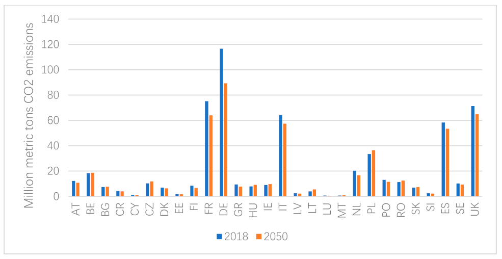
Given all assumptions, the calculated total CO2 emissions in 2018 amount to 590 million metric tons, which corresponds to 54% of total emissions from the transport sector in 2018 (1095 million metric tons) as reported by EEA [2]. This is below the share of emissions from light-duty vehicles reported by EEA [2], which amounted to 60% of the emissions from the transport sector. Five countries, France, Germany, Italy, Spain and UK, together accounted for 65% of total emissions (Figure 2). The calculated total emissions in 2050 amounted to 534 million tonnes of CO2 in the member states of EU and UK, which corresponded to a decrease in emissions of CO2 by 9% from the 2018 emission level. Emissions decreased over time in most countries (Figure 2).
Five countries (France, Germany, Italy, Spain and UK) accounted for approximately 2/3 of total emissions in both years. All these countries show a decline in emissions from 2018 to 2050, but the emissions from several other countries increase (Czech Republic, Belgium, Bulgaria, Hungary, Ireland, Lithuania, Malta, Poland, Romania and Slovakia) because of the predicted increase in travel demand.
3.2. Costs and Interest Rate
Costs were calculated as changes in consumer surplus from deviations in the purchases of new cars from the business-as-usual (BAU) level. Linear demand functions were assumed, and changes in consumer surplus were calculated by means of data on business-as-usual quantities and prices of new passenger cars, and the price elasticity of the new passenger car demand. To the best of the authors’ knowledge, there was no study with elasticity estimates for individual EU-28 countries disaggregated into each vehicle type (see review in Graham and Glaister [35]). One study estimated price elasticities of the different car types in Norway [36], the results of which will be used in the present study. According to Fridström and Östli [36], the elasticities of the cars were; electric cars −0.99, plug in hybrids −1.72, ordinary hybrids −0.97, diesel cars −1.27 and gasoline cars −1.08. Since the present study makes no distinction between different types of hybrid and fossil fuel cars, the averages of the price elasticities were used, which gave −1.35 for hybrids and −1.14 for fossil fuel cars.
New vehicle price data were obtained from Aklilu [27] who reported the prices in 2016 euros. These prices were updated to 2018 prices using country specific consumer price index [37]. In 2018, the average price of a passenger car inclusive of tax was approximately 29,600 euro for fossil fuel-driven cars, 39,700 for hybrid cars and 51,300 for electric cars. As shown in Appendix A, this difference in price levels raises the cost in terms of changes in consumer surplus of a shift from fossil fuel cars to the other cars.
Generally, the price of new passenger cars has been rising in the last decade. Prices of hybrid and electric cars relative to fossil fuel cars rose in the early 2000s and since then have on average been decreasing [19]. In the business-as-usual data in 2018, the average EU relative price of hybrid cars to fossil fuel cars is about 1.34 and 1.73 for electric cars to fossil fuel cars. It is assumed that the relative prices will approach 1 from 2030 onwards as a result of investment in research, development and demonstration, plus learning-by-doing (e.g., [8,38,39,40]). This assumption implies that the average annual price decrease of hybrid cars and electric cars is 2.05% and 3.83%, respectively, which were used in this study.
The future cost of achieving emission reductions from passenger cars in the EU and UK was discounted at 3%. This rate is similar to the one used by Bosetti and Longden [8], but falls between the rates used in Stern [41] and Nordhaus [42], which extensively discuss the ethics and consequences of the discount rate used in the economics of climate change with intergenerational outcomes.
3.3. Emission Reduction Targets
The main focus in this study is on the emission target of a 60% reduction of the emissions in 1990 from the transport sector to be achieved by 2050. According to EEA [1], emissions from the transport sector in 1990 amounted to approximately 862 million metric tons of CO2, which implies a maximum of 345 million metric tons of CO2 by 2050 for the transport sector. Predicted reference emission from transports in 2050 amounts to 957 million tonnes [4]. The necessary reduction to achieve the target in 2050 is then 64% from the transport sector. In a cost-effective solution, the reduction of emissions from light-duty cars depends on the marginal abatement cost compared with other transport modes (heavy-duty cars, aviation, shipping, etc.) Therefore, calculations of costs are made for different levels of emission reductions from the projected level of 534 million tonnes in 2050.
4. Scenarios on Future Travel Demand and Carbon Efficiency
Several assumptions were made regarding future development of travel demand and carbon efficiency. In the reference scenario, costs were calculated for the assumed annual rates of changes displayed in Appendix B Table A4. In addition, costs were calculated for alternative scenarios on future development of these rates. The expected increase in travel demand was regarded as an impediment to achieve emission reductions from the transport sector (e.g., [5]). Cost calculations were therefore made for a decrease by 50% in the rate of increase in travel demand for all countries.
When electric vehicles are coupled with grid decarbonization, their emission reduction potential can be further enhanced [43]. The increase in carbon efficiency in the electricity production is higher than that in the transport sector in all EU member states and the EU [4]. The average annual increase amounts to 0.017, which can be compared with the annual rate of increase in the transport sector of 0.009. If the infrastructure for loading electricity is improved at the same rate as the carbon efficiency in the electricity production the carbon efficiency can increase at a higher rate for electric and hybrid cars than for fossil fuel vehicles, in particular for countries with high reliance on fossil fuels for electricity production. Therefore, the rate of increase in carbon efficiency in electric cars is assumed to be the same as for electricity production in an alternative scenario. Similar to the assumption for carbon efficiency level, it is assumed that the rate of increase for hybrid cars corresponds to the average of that for electricity production and fossil fuel vehicles.
In addition to scenarios on separate changes in annual rates of demand and carbon efficiency, costs are calculated for a combination of these two with decrease in travel demand and increase in carbon efficiency. In total, calculations of costs were then made for four different scenarios defined in Table 1.
5. Results
5.1. Cost-Effective Solutions
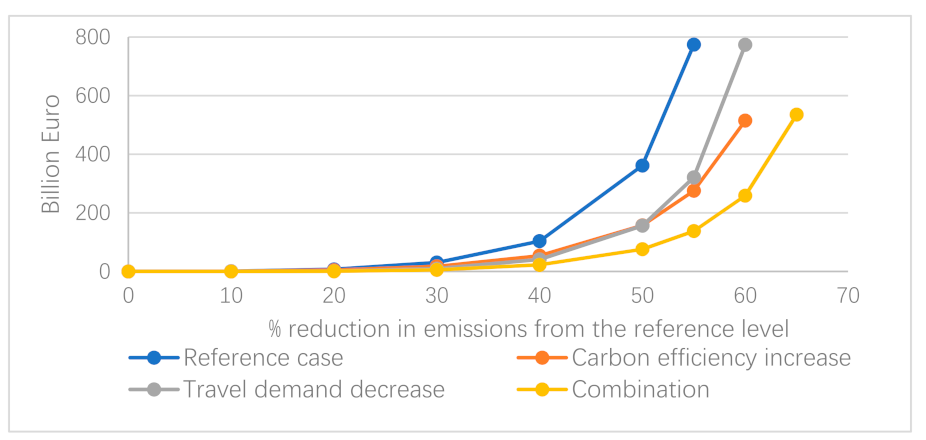
The numerical dynamic optimization model is non-linear, includes 28 countries, 32 time periods and 3 different vehicles choices, which requires a powerful model system for mathematical optimization. Therefore, the GAMS CONOPT solver [44] was used to calculate minimum costs for different reduction levels in the reference emissions in 2050 of 534 million tonnes of CO2. The cost-effective allocation of annuals cost for different emission reduction differed considerably among the four scenarios (Figure 3).
The difference in costs between the scenarios was mainly explained by the decrease in emission in year 2050 in travel demand. A lower rate of increase in travel demand reduced emissions in 2050 by 8.4% compared with the reference case. However, the composition of vehicles shows a modest change with an increase of non-fossil fuel cars from approximately 3% to 7% because of the price reduction. The reduction in emission in the carbon efficiency scenario was thus small, 0.5% from the reference level. The lower cost of emission reduction in the scenario was explained by the higher increase in carbon efficiency in the electricity sector compared with the transport sector.
Common to all scenarios is the relatively rapid increase in costs at reduction levels exceeding 40%, i.e., above 213 million tonnes. This level coincides with a proportional reduction between the light and heavy duty cars for achieving the EU target of maximum emissions from the transport sector of 345 million metric tons. The light duty vehicles account for approximately 60% of the emission from transport, and a proportional reduction would imply an emission target of 207 million tonnes. At this level, the annual cost ranged between 23 and 103 million euro depending on scenario, which corresponded to 0.13% and 0.60%, respectively, of the average annual predicted EU GDP. The upper level can be regarded as relatively high when compared with the cost estimates of achieving the 2050 climate targets, which ranges from 0.1% to 0.9% of EU GDP [45].
The average reduction cost at the 40% emission reduction level varied between 106 and 484 euro/metric ton CO2 depending on the scenario. This can be compared with the result obtained by Van Vliet [46], which shows that the average abatement cost using hybrid and electric cars ranges from 400 to 1900 euros per metric ton of CO2. Kok et al. [7] review studies of greenhouse gas mitigation in transport in the US and EU, and present the cost of GHG abatement under cost-effectiveness to be approximately 400 euro/metric ton of GHG in 2018 euro.
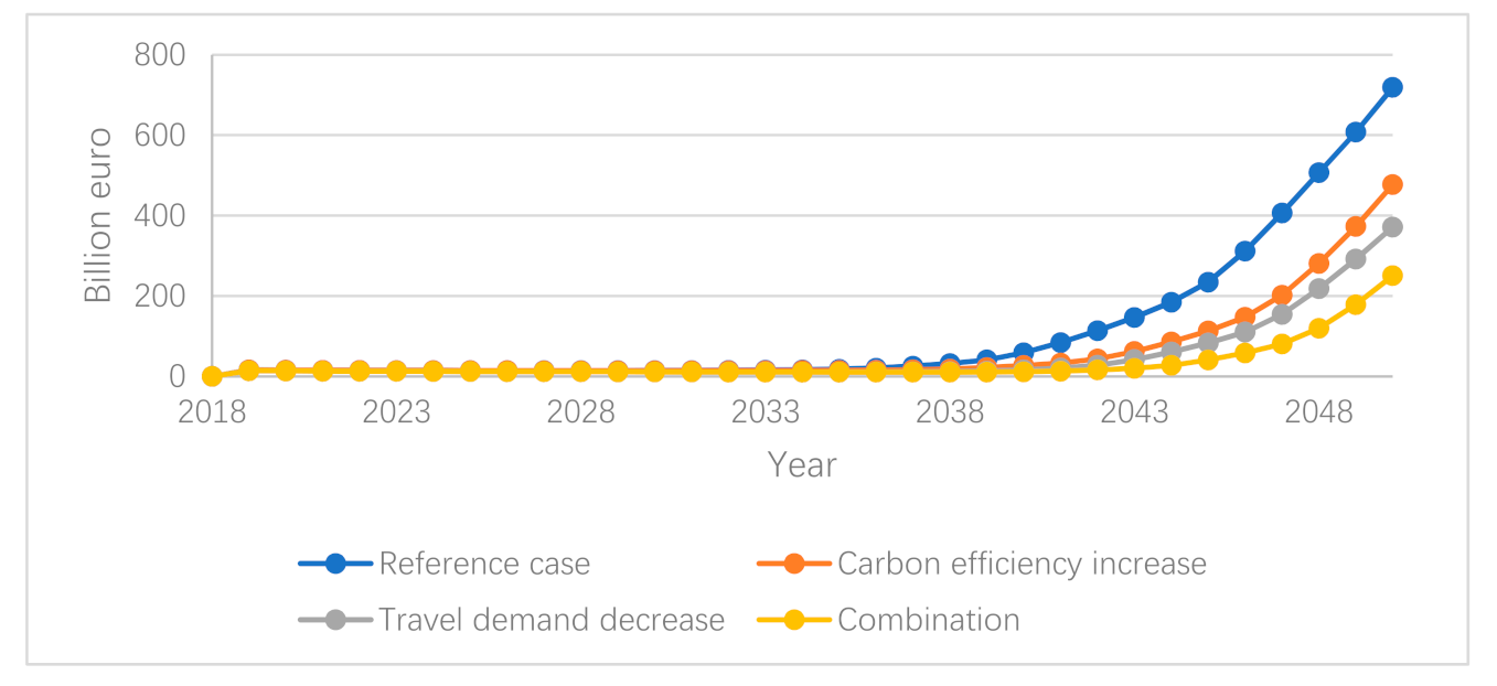
As expected, the annual costs increase over time because of the discount rate, travel demand decreased and/or carbon efficiency increased at all emission reduction targets. This is shown for the 40% emission reduction level in Figure 4.
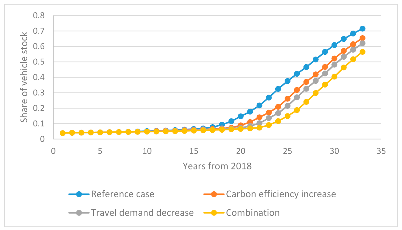
The curves in Figure 4 show the impacts of decreased travel demand, which not only reduces cost because of ‘free of charge’ emission reduction, but also from a delay in expenses compared with the references case. Such delay reduces cost in present terms. A similar impact is obtained by increased carbon efficiency, which creates incentives for delays in abatement to reach the target. Annual costs start to increase in year 22 in the reference case and in year 27 in the combined scenario. This reflects expenses for the increase in the share of non-fossil fuel cars, which increases from approximately 0.03 in the start year to 0.72 of the total vehicle stocks in the reference case in the final year and to 0.56 in the combined scenario (Appendix B Figure A2) at the 40% emission reduction level.
5.2. Distributional Effects
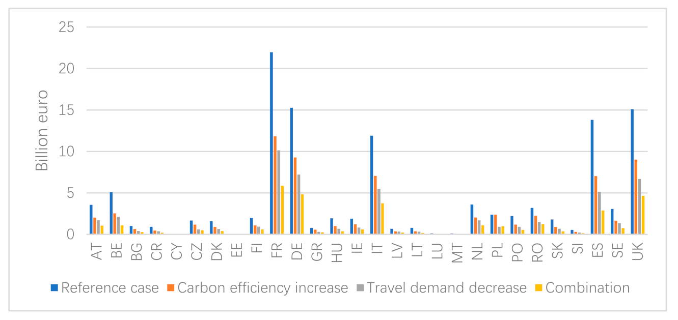
With respect to the allocation of costs among countries, they are highest for countries with relatively large emissions (Figure 5).
Five countries—Germany, the UK, France, Italy and Spain—account for approximately 2/3 of total costs in all scenarios. However, whether or not this allocation is regressive or progressive depends on the relation to income. When the proportional allocation of costs is low (high) for countries with low (high) share of total EU income, the cost allocation is progressive (regressive). In general, regressive allocation of cost burdens is regarded as unfair, which has guided the allocation of effort sharing commitments under the EU 2030 emission target (EC, 2011).
The results in the literature on the progressivity or regressivity of climate policies in the transport sector are mixed (see reviews in [11,16]). A meta regression analysis of studies on distributional effects of climate polices indicated that they are progressive in the transport sector [47]. A common result from the reviews and meta regression analysis is that the choice of reference point of the cost, annual income or lifetime income can affect the outcome. Similar to the present study, several studies calculate costs as changes in consumer surplus. Unlike this study, distributional outcomes are calculated for economic instruments mainly on fuel. The changes in consumer surplus then include increases in costs for actual fuel use and welfare loss from reductions in fuel use. The present study includes only the welfare loss since charges/subsidies are regarded as transfer and not as a social cost although it is a real cost for the car owner. Therefore, costs are related to total income measured as GDP. For comparative purposes, costs are also related to annual consumption expenditures), which is often used as a proxy for lifetime incomes. For both reference bases, annual averages are calculated based on predictions from 2018 to 2050 (Appendix B Table A5). The calculated Suits index shows small differences between the reference points and the scenarios (Table 2).
The calculated Suits index shows that the cost-effective allocation is almost neutral, it fluctuated between −0.037 and 0.024 depending on the scenario and reference point. It is slightly progressive in the travel demand scenario since the reduction in the rate of increase demand reduced the cost burden on relatively low income countries with high travel demand increases. The regressive effect was highest for the carbon efficiency scenario because of the assumed increases in the rate of decarbonization in high income countries with large shares of the total income and costs.
The calculated Suits indices were relatively low in absolute terms when compared with estimates of Suits index for gasoline tax in the US, which varied between −0.16 and −0.36 depending on population group [48]. The estimates are in line with some results obtained by Sterner [11] for gasoline taxes in seven European countries, where the Suits index for regressive outcomes within the countries ranged between −0.002 and −0.178. The calculations in this study are also close to the results by Eliasson et al. [14] who found a slight regressive climate tax on cars in Sweden, ranging between −0.03 and −0.08 depending on the design of the tax.
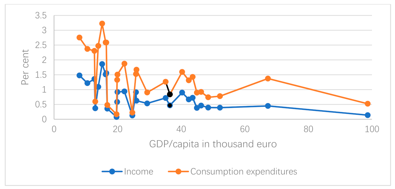
The Suits index was much affected by the five countries with the largest emissions, which accounted for approximately 2/3 of the total cost in all scenarios. This may hide the distributional impacts as measured by the share of costs related to income or consumption expenditures, which is shown for the reference scenario in Figure 6.
The EU MS and UK average income as measured by GDP/capita amounted to 30.3 thousand euro, and the average cost share was 0.58% and 1.07% of total income and consumption expenditures, respectively. The income in a majority of the countries (17) is below the average EU and UK GDP/capita. The lowest income levels are found in Bulgaria and Croatia and the highest in Ireland and Luxemburg. Both reference points show the same pattern; low income countries as measured by GDP/capita have a disproportionally high share of costs. Both highest and lowest cost shares are found at incomes below the average. When consumption expenditure is the reference point, the cost can reach 3.2% and several countries face higher cost shares than the EU and UK average of 1.07%.
6. Discussion and Conclusions
This study estimated the minimum cost of reducing CO2 emission in 2050 from passenger cars in the EU MS and UK. As such, eventual transaction costs of implementing policies to reach the emission reductions were not included, such as costs for land use planning (e.g., [49]). Costs were measured as changes in consumer surplus from the reference emission. A numerical dynamic cost minimization model was constructed, which allowed for country specific annual changes in travel demand, carbon efficiency and decrease in prices of hybrid and electric cars. Such a numerical model has not been constructed before. The minimum cost in the reference case amounted to 103 billion euro, which corresponded to approximately 0.6% of total EU GDP in 2018. The costs were reduced considerably, to 0.13% of total EU GDP, when the increase in travel demand was reduced by one half, and when carbon efficiency by electric cars increased at the same rate as decarbonization of electricity production. Cost allocations for cost-effective solutions to an emission reduction by 40% were slightly regressive in most cases but progressive with lower annual increase in travel demand.
The cost estimates were sensitive, not only to assumptions on development of travel demand and carbon efficiency, but also to the chosen parameter values on interest rate and price decreases on electric and hybrid cars. A decrease in the interest rate from 3% to 2% raises the total cost by approximately 30% with small differences between the scenarios (Table 3).
A 30% higher rate of decrease in prices of non-fossil fuels reduced total cost between 17 and 22% depending on scenario, and a reduction in the price elasticity of cars by 30% increased costs by approximately 43% in all scenarios.
Factors not included in the study will also affect the results, such as transfer of firms’ costs for technological development to customers. Such transfer can increase the price of passenger cars, while technology development itself has price-reducing effects. Another crucial assumption is that on given car prices and developments in carbon efficiency. EU motor vehicle manufacturers account for approximately 25% of the global sales of new cars, with almost 30% of the production in the EU exported to non-EU countries [50]. The imported share of sales of new vehicles is approximately 23%. Market prices are therefore likely to respond to the switch from fossil fuel to hybrid and electric cars. Neglect of these adjustments implies an overestimation of the cost of reducing demand for fossil fuel cars if the price is reduced. However, the costs of hybrid and electric cars are underestimated if the increase in demand results in higher prices. The magnitude of these impacts is determined by the EU passenger car market, which is characterized by oligopolistic competition with product differentiation that might give little room for demand change to affect prices [51].
Another assumption was that the elasticity is the same across the EU-27 countries and UK for each of the car types due to a lack of studies that estimate the price elasticity of passenger cars for each country and vehicle type. However, in reality, the price elasticity of passenger car demand may be different across the three types of vehicles, and future studies using disaggregated elasticities may improve the precision of the calculated cost.
Despite all shortcomings of the numerical model, the cost estimates are relatively close to the results from other studies at the 40% reduction level in emissions from passenger cars, which corresponds to its share of the EU reduction requirement in the transport sector. A new result is the differences in cost burdens among countries, which ranges between 0.2% and 3.2% of consumption expenditures. This may be an impediment for the implementation of a cost effective emission reduction at the EU level. The variation is smaller for the five countries with the highest emissions, which may facilitate vehicle transformation in these countries. The results also indicate that the costs increased rapidly for higher reduction in emission from passenger cars. The cost increased by at least 200% in all scenarios when the reduction requirement increased from 40 to 50%. This raises the question if it is less costly to reduce emissions from light-duty vehicles than to reduce emissions by a higher level from heavy-duty cars or other transport modes to obtain the overall reduction of 60% for the transport sector without serious distributional effects? A response to this requires cost-effectiveness and equity analysis of the entire transport sectors, which remains to be made.
Author Contributions
Conceptualization I.-M.G.; methodology I.-M.G. and I.-M.G.; validation I.-M.G. and A.Z.A.; formal analysis I.-M.G. and A.Z.A.; data curation A.Z.A.; writing—original version I.-M.G. and A.Z.A.; writing—review editing I.-M.G. and A.Z.A. All authors have read and agreed to the published version of the manuscript.
Funding
This research received no external funding.
Institutional Review Board Statement
Not applicable.
Informed Consent Statement
Not applicable.
Data Availability Statement
All data is reported in the article.
Conflicts of Interest
The authors declare no conflict of interest.
Appendix A. Derivation of Cost Functions and First-Order Conditions
Appendix A.1. Cost Functions
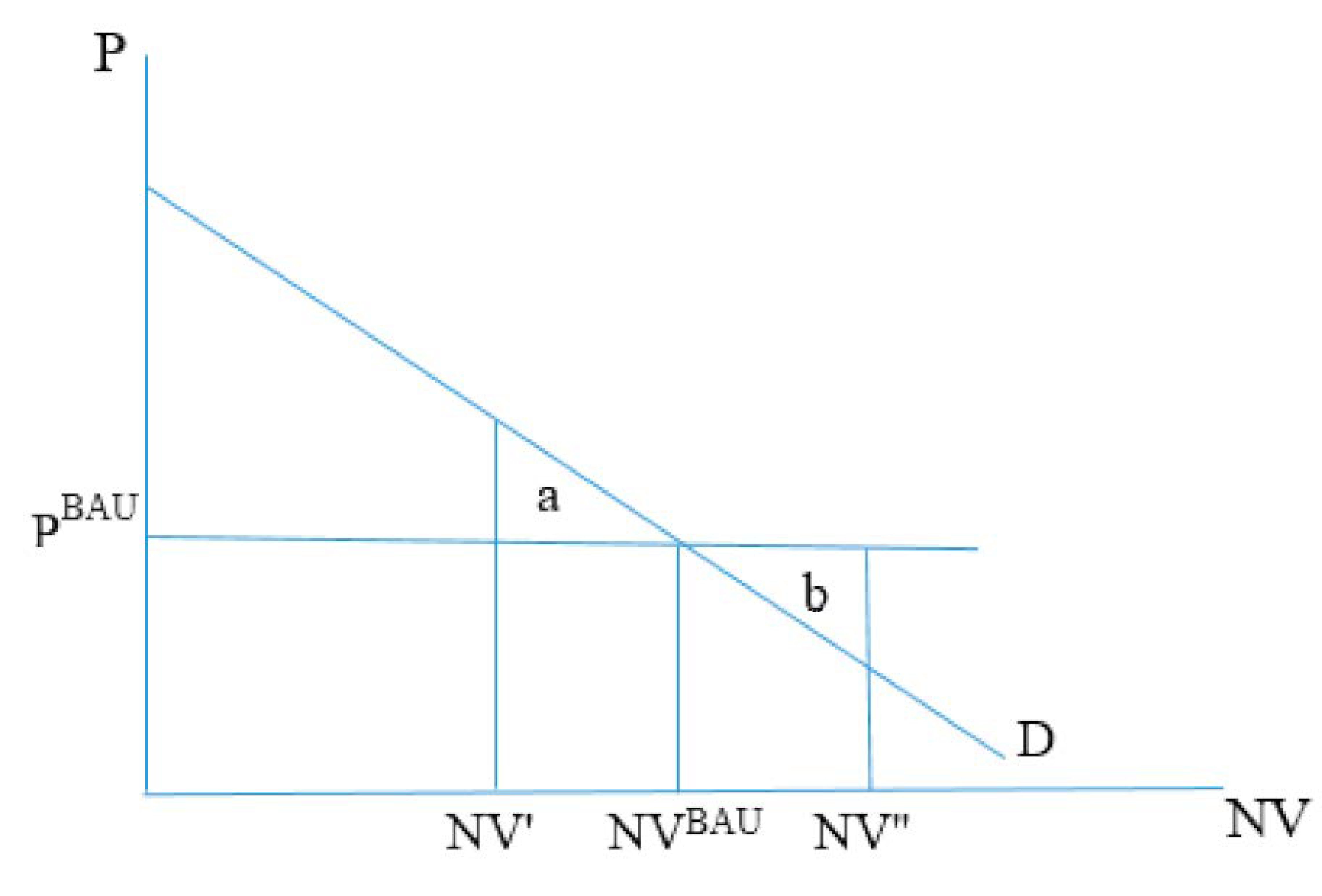
The cost function is defined as the change in consumer surplus from the BAU level of new cars, which is illustrated in Figure A1.
Figure A1.
Illustration of calculations of changes in consumer surplus.

The curve illustrates the inverted demand for , and and are the BAU levels of the price and respectively. The deviations from can be either positive or negative. The reduction in consumer surplus from the reduction to is shown by the area denoted , and the reduction at a higher level than is illustrated by the area .
In order to derive the consumer surplus, a linear demand of vehicles was assumed as:
where is the intercept term of the demand curve and is the slope. The intercept and the slope are derived from the definition of the demand elasticity:
where is the price elasticity of vehicle demand, and and are the observed number of vehicles and price with business as usual at the beginning of the policy period. Using the above equation, the intercept is:
The inverse demand function in terms of observable and exogenous parameters is:
The change in consumer surplus, , is calculated by integrating the inverse demand function from to and subtracting the area as illustrated in Figure A1, which gives:
The consumer surplus change for each vehicle type in each of the EU-28 countries in each period of time is:
When calculating the impact on costs of increases in travel demand, the demand function is assumed to have an unchanged slope evaluated at the BAU price and vehicle demand levels, and to shift outwards because of the increased demand. The BAU demand level thus increases at the same rate as the increase in income. The coefficient in the inverted demand function, , is then obtained from Equation (A2), which gives the change in consumer surplus when demand increases at the annual rate of as:
Appendix A.2. First-Order Conditions
The optimization problem in Equation (6) is solved by constructing the Lagrange expression, which is written as:
where and ≥ 0 are the Lagrange multipliers on the emission and travel demand constraints, respectively. In order to facilitate calculations and interpretations of the model results, the simple difference equation in (1) is integrated to obtain:
The necessary first-order conditions with respect to are written as:
Equation (A10) establishes that the marginal cost of a new passenger car type, the first expression on the right-hand side of (A10) in brackets, is equal to the marginal impact on the future emission target and on the contribution to current and future travel demand. The marginal impact on the future emission target is determined by , which shows the impact on emissions at time from a marginal increase in weighted with the shadow cost, , of the emission constraint. A low depreciation rate and/or low fuel efficiency improvement gives a relatively large impact and vice versa. Similarly, the marginal impact on current and future travel demand is given by , which is interpreted as the contribution of a marginal to current and future travel demand with an annual weighting by the Lagrange multiplier .
Cost-effectiveness implies that the marginal cost of vehicles is the same for all countries and vehicle types in 2050 and equals θ, which is derived from Equation (A9).
Appendix B

Table A1.
Passenger car stock and number of new passenger cars in 2018.
| Passenger Car Stock | Number of New Passenger Car | |||||
|---|---|---|---|---|---|---|
| Country | Fossil Fuel | Hybrid | Electric | Fossil Fuel | Hybrid | Electric |
| Austria | 4951.00 | 6.17 | 20.83 | 333.00 | 4.04 | 3.96 |
| Belgium | 5800.00 | 43.76 | 9.24 | 549.00 | 4.24 | 3.76 |
| Bulgaria | 2740.20 | 30.13 | 2.67 | 244.63 | 11.98 | 1.40 |
| Croatia | 1600.00 | 65.54 | 0.46 | 138.00 | 9.18 | 1.82 |
| Cyprus | 549.00 | 7.89 | 0.11 | 18.00 | 22.97 | 0.03 |
| Czechia | 5728.00 | 16.52 | 2.48 | 246.62 | 12.07 | 0.30 |
| Denmark | 2583.00 | 0.96 | 10.04 | 213.00 | 3.32 | 1.68 |
| Estonia | 743.00 | 1.75 | 1.25 | 26.00 | 0.92 | 0.08 |
| Finland | 3457.00 | 10.50 | 2.50 | 118.00 | 1.22 | 0.78 |
| France | 31,447.59 | 471.41 | 115.00 | 2104.00 | 3.06 | 30.95 |
| Germany | 46,984.00 | 27.83 | 83.18 | 3253.00 | 145.94 | 36.06 |
| Greece | 5173.07 | 57.55 | 4.38 | 304.36 | 14.90 | 1.74 |
| Hungary | 3576.00 | 61.16 | 3.84 | 280.00 | 13.01 | 1.99 |
| Ireland | 2140.00 | 37.39 | 4.61 | 119.00 | 7.75 | 1.25 |
| Italy | 35,644.00 | 3361.84 | 12.16 | 1787.98 a | 141.03 a | 15.00 a |
| Latvia | 656.00 | 130.56 | 0.44 | 16.00 | 0.92 | 0.08 |
| Lithuania | 1313.00 | 116.04 | 0.97 | 166.00 | 2.66 | 0.34 |
| Luxembourg | 411.00 | 2.64 | 1.36 | 49.02 | 2.56 | 0.42 |
| Malta | 377.00 | 22.32 | 0.68 | 19.00 | 0.96 | 0.04 |
| Netherlands | 8427.48 | 95.55 | 6.98 | 403.00 | 3.04 | 7.96 |
| Poland | 19,706.00 | 3719.98 | 3.02 | 1219.00 a | 115.78 a | 1.22 a |
| Portugal | 5216.00 | 56.02 | 9.98 | 221.00 | 79.54 | 4.46 |
| Romania | 6350.00 | 190.90 | 1.10 | 126.00 | 3.00 | 1.00 |
| Slovakia | 2293.54 | 25.65 | 1.80 | 160.24 | 7.85 | 0.91 |
| Slovenia | 1126.00 | 15.61 | 1.39 | 71.00 | 2.48 | 0.52 |
| Spain | 24,082.00 | 765.92 | 26.08 | 1390.00 | 22.71 | 11.29 |
| Sweden | 4598.00 | 254.34 | 16.66 | 353.00 | 4.85 | 7.15 |
| United Kingdom | 31,100.07 | 361.60 | 55.34 | 2325.00 | 0.42 | 15.58 |
| Total | 258,771.90 | 9957.50 | 398.55 | 17,047.00 | 642.40 | 151.75 |
Table A2.
Traffic load per passenger car in kilometers and emissions of CO2 kg/km for different vehicle types in 2018.
Table A2.
Traffic load per passenger car in kilometers and emissions of CO2 kg/km for different vehicle types in 2018.
| Country | Km Per Passenger Car | CO2 kg/km; Fossil Fuel d Hybrid e Electric a | ||
|---|---|---|---|---|
| Austria | 16,431 | 0.404 | 0.213 | 0.022 |
| Belgium | 17,560 a | 0.255 | 0.145 | 0.035 |
| Bulgaria | 14,937 a | 0.156 | 0.134 | 0.112 |
| Croatia | 15,363 | 0.262 | 0.158 | 0.053 |
| Cyprus | 10,915 a | 0.353 | 0.244 | 0.135 |
| Czechia | 13,567 | 0.333 | 0.223 | 0.114 |
| Denmark | 26,375 | 0.299 | 0.187 | 0.076 |
| Estonia | 14,773 a | 0.221 | 0.212 | 0.204 |
| Finland | 19,268 | 0.237 | 0.143 | 0.049 |
| France | 23,634 | 0.200 | 0.106 | 0.012 |
| Germany | 19,593 | 0.294 | 0.193 | 0.092 |
| Greece | 10,047 b | 0.204 | 0.159 | 0.115 |
| Hungary | 17,563 | 0.301 | 0.187 | 0.074 |
| Ireland | 23,159 a | 0.242 | 0.160 | 0.078 |
| Italy | 18,527 | 0.228 | 0.140 | 0.052 |
| Latvia | 19,385 | 0.230 | 0.142 | 0.055 |
| Lithuania | 21,062 | 0.261 | 0.164 | 0.066 |
| Luxembourg | 9666 a | 1.503 | 0.763 | 0.022 |
| Malta | 10,412 a | 0.184 | 0.160 | 0.135 |
| Netherlands | 16,260 | 0.212 | 0.153 | 0.095 |
| Poland | 9105 | 0.216 | 0.200 | 0.184 |
| Portugal | 13,857 a | 0.229 | 0.139 | 0.049 |
| Romania | 9756 a | 0.321 | 0.196 | 0.070 |
| Slovakia | 16,786 a | 0.180 | 0.109 | 0.035 |
| Slovenia | 8935 | 0.420 | 0.240 | 0.059 |
| Spain | 12,766 | 0.673 | 0.358 | 0.042 |
| Sweden | 12,040 c | 0.312 | 0.160 | 0.008 |
| United Kingdom | 21,180 | 0.229 | 0.139 | 0.048 |
Table A3.
Average passenger car price inclusive of tax in euros per vehicle energy type, thousand euro in 2018.
Table A3.
Average passenger car price inclusive of tax in euros per vehicle energy type, thousand euro in 2018.
| Fossil Fuel | Hybrid | Electric | |
|---|---|---|---|
| Austria | 31.249 | 40.600 | 49.282 |
| Belgium | 28.349 | 38.765 | 49.667 |
| Bulgaria c | 29.987 | 40.041 | 51.561 |
| Croatia c | 29.333 | 39.168 | 50.438 |
| Cyprus c | 29.141 | 38.911 | 50.107 |
| Czechia c | 29.907 | 39.933 | 51.423 |
| Denmark | 36.374 | 46.071 | 57.326 |
| Estonia c | 30.569 | 40.818 | 52.563 |
| Finland | 32.467 | 44.272 | 57.209 |
| France | 26.591 | 38.029 | 51.510 |
| Germany | 32.303 | 42.045 | 54.553 |
| Greece | 22.367 | 32.983 | 45.561 |
| Hungary c | 30.082 | 40.167 | 51.724 |
| Ireland | 27.102 | 35.512 | 46.698 |
| Italy | 23.901 | 33.052 | 44.162 |
| Latvia c | 30.160 | 40.271 | 51.859 |
| Lithuania c | 30.441 | 40.647 | 52.342 |
| Luxembourg | 34.753 | 43.276 | 53.945 |
| Malta c | 29.302 | 39.127 | 50.384 |
| Netherlands | 28.738 | 39.830 | 52.016 |
| Poland c | 29.699 | 39.656 | 51.066 |
| Portugal | 28.145 | 38.252 | 50.400 |
| Romania c | 30.299 | 40.458 | 52.098 |
| Slovakia c | 29.680 | 39.630 | 51.033 |
| Slovenia c | 29.489 | 39.376 | 50.705 |
| Spain | 26.145 | 36.054 | 48.147 |
| Sweden | 33.195 | 42.505 | 54.148 |
| United Kingdom | 31.248 | 42.164 | 54.664 |
Table A4.
Annual rate of increase in travel demand, carbon efficiency in the transport sector, depreciation and carbon efficiency in electricity production.
Table A4.
Annual rate of increase in travel demand, carbon efficiency in the transport sector, depreciation and carbon efficiency in electricity production.
| Travel Demand a | Carbon Efficiency in Transport a | Depreciation of Cars a | Efficiency in Electricity Production a | |
|---|---|---|---|---|
| Austria | 0.006 | 0.008 | 0.122 | 0.012 |
| Belgium | 0.007 | 0.006 | 0.111 | 0.006 |
| Bulgaria b | 0.005 | 0.006 | 0.067 | 0.020 |
| Croatia b | 0.007 | 0.008 | 0.081 | 0.017 |
| Cyprus b | 0.009 | 0.010 | 0.067 | 0.012 |
| Czechia b | 0.012 | 0.008 | 0.071 | 0.020 |
| Denmark | 0.007 | 0.009 | 0.114 | 0.018 |
| Estonia b | 0.005 | 0.009 | 0.060 | 0.019 |
| Finland | 0.003 | 0.009 | 0.083 | 0.018 |
| France | 0.005 | 0.009 | 0.111 | 0.017 |
| Germany | 0.003 | 0.010 | 0.105 | 0.017 |
| Greece | 0.002 | 0.008 | 0.064 | 0.021 |
| Hungary b | 0.012 | 0.007 | 0.070 | 0.018 |
| Ireland | 0.012 | 0.007 | 0.119 | 0.016 |
| Italy | 0.004 | 0.007 | 0.088 | 0.017 |
| Latvia b | 0.004 | 0.009 | 0.077 | 0.008 |
| Lithuania b | 0.003 | 0.008 | 0.059 | 0.017 |
| Luxembourg | 0.002 | 0.006 | 0.156 | 0.012 |
| Malta b | 0.014 | 0.007 | 0.093 | 0.006 |
| Netherlands | 0.005 | 0.010 | 0.094 | 0.012 |
| Poland b | 0.011 | 0.009 | 0.072 | 0.020 |
| Portugal | 0.008 | 0.008 | 0.078 | 0.021 |
| Romania b | 0.011 | 0.008 | 0.061 | 0.021 |
| Slovakia b | 0.009 | 0.007 | 0.074 | 0.017 |
| Slovenia b | 0.007 | 0.009 | 0.099 | 0.021 |
| Spain | 0.009 | 0.011 | 0.081 | 0.020 |
| Sweden | 0.006 | 0.009 | 0.101 | 0.010 |
| United Kingdom | 0.007 | 0.009 | 0.125 | 0.015 |
Table A5.
GDP, consumption expenditures, annual rate of increase in GDP and consumption expenditures from 2018 to 2020, and GDP/capita in 2018 euro.
Table A5.
GDP, consumption expenditures, annual rate of increase in GDP and consumption expenditures from 2018 to 2020, and GDP/capita in 2018 euro.
| Country | GDP Bill Euro a | Consumption Expenditure b | GDP Increase c | Cons. Exp. Increase c | GDP/Capita, Thousand Euro d |
|---|---|---|---|---|---|
| Austria | 385 | 200 | 0.0152 | 0.0134 | 43.60 |
| Belgium | 460 | 238 | 0.0187 | 0.0135 | 40.29 |
| Bulgaria c | 56 | 34 | 0.0135 | 0.022 | 8.00 |
| Croatia c | 52 | 30 | 0.0159 | 0.0199 | 12.70 |
| Cyprus c | 21 | 14 | 0.0228 | 0.015 | 24.63 |
| Czechia c | 211 | 100 | 0.0168 | 0.0191 | 19.85 |
| Denmark | 302 | 141 | 0.0184 | 0.0169 | 52.19 |
| Estonia c | 26 | 13 | 0.0131 | 0.0216 | 19.66 |
| Finland | 233 | 124 | 0.0157 | 0.0143 | 42.37 |
| France | 2360 | 1272 | 0.0162 | 0.0135 | 35.10 |
| Germany | 3356 | 1755 | 0.0091 | 0.0142 | 48.48 |
| Greece | 180 | 124 | 0.012 | 0.0131 | 16.76 |
| Hungary c | 136 | 67 | 0.0166 | 0.0186 | 13.91 |
| Ireland | 327 | 99 | 0.0161 | 0.0214 | 67.27 |
| Italy | 1771 | 1066 | 0.0142 | 0.0124 | 29.30 |
| Latvia c | 29 | 17 | 0.0138 | 0.0023 | 15.13 |
| Lithuania c | 45 | 28 | 0.0092 | 0.0021 | 16.24 |
| Luxembourg | 60 | 19 | 0.0274 | 0.0127 | 98.64 |
| Malta c | 13 | 5 | 0.0188 | 0.0191 | 25.94 |
| Netherlands | 774 | 341 | 0.0124 | 0.0153 | 44.92 |
| Poland c | 498 | 290 | 0.016 | 0.02 | 12.96 |
| Portugal | 205 | 132 | 0.0109 | 0.016 | 19.95 |
| Romania c | 204 | 138 | 0.0158 | 0.02 | 10.50 |
| Slovakia c | 90 | 50 | 0.0159 | 0.022 | 16.44 |
| Slovenia c | 46 | 24 | 0.0139 | 0.017 | 22.13 |
| Spain | 1204 | 700 | 0.0144 | 0.015 | 25.77 |
| Sweden | 471 | 215 | 0.0212 | 0.0173 | 46.26 |
| United Kingdom | 2420 | 1566 | 0.0177 | 0.0139 | 36.44 |
Table A6.
Sensitivity analysis with cost estimates for reaching 40% emission reductions by 2050 with changes in discount rate, price of new cars and the car price elasticity, billion Euro.
Table A6.
Sensitivity analysis with cost estimates for reaching 40% emission reductions by 2050 with changes in discount rate, price of new cars and the car price elasticity, billion Euro.
| Reference Case | Carbon Efficiency Increase | Travel Demand Decrease | Combination | |
|---|---|---|---|---|
| No changes | 4024 | 2291 | 1768 | 1124 |
| Discount rate reduced from 0.03 to 0.03 | 5320 | 3016 | 2327 | 1462 |
| Price decrease by 30% | 2910 | 1717 | 1316 | 877 |
| Decrease in car price elasticity by 30% | 5749 | 3273 | 2526 | 1606 |
Figure A2.
Hybrid and electric vehicles in cost-effective solutions under different scenarios at 40% CO2 emission reduction, share of total vehicle stock.
Figure A2.
Hybrid and electric vehicles in cost-effective solutions under different scenarios at 40% CO2 emission reduction, share of total vehicle stock.

References
- EEA. Greenhouse Gases from the Transport Sector in the EU. 2020. Available online: https://www.eea.europa.eu/data-and-maps/indicators/transport-emissions-of-greenhouse-gases-7/assessment (accessed on 24 February 2021).
- EEA. Share of Transport Greenhouse Gas Emissions. 2021. Available online: https://www.eea.europa.eu/data-and-maps/daviz/share-of-transport-ghg-emissions-2#tab-googlechartid_chart_12 (accessed on 24 February 2021).
- EC. Roadmap to a Single European Transport Area—Towards a Competitive and Resource Efficient Transport System, COM (2011) 144 final of 28 March 2011; White Paper; EC: Brussels, Belgium, 2011. [Google Scholar]
- EC. EU Reference Scenario 2016. 2016. Available online: https://ec.europa.eu/energy/data-analysis/energy-modelling/eu-reference-scenario-2016_en (accessed on 23 February 2021).
- Krause, J.; Thiel, C.; Tsokolos, D.; Samaras, Z.; Rota, C.; Ward, A.; Prenningen, P.; Coosemans, T.; Neugebauer, S. EU road vehicle energy consumption and CO2 emissions by 2050—Expert based scenarios. Energy Policy 2020, 138, 111224. [Google Scholar] [CrossRef]
- Eurostat. Passenger Car by Type of Motor Energy. 2021. Available online: https://ec.europa.eu/eurostat/databrowser/view/road_eqs_carpda/default/table?lang=en (accessed on 28 February 2021).
- Kok, R.; Annema, J.A.; van Wee, B. Cost-effectiveness of greenhouse gas mitigation in transport: A review of methodological approaches and their impact. Energy Policy 2011, 39, 7776–7793. [Google Scholar] [CrossRef]
- Bosetti, V.; Longden, T. Light duty vehicle transportation and global climate policy: The importance of electric drive vehicles. Energy Policy 2013, 58, 209–219. [Google Scholar] [CrossRef] [Green Version]
- Kallbekken, S.; Saelen, H. Public acceptance for environmental taxes: Self-interest and distributional concerns. Energy Policy 2011, 39, 2966–2973. [Google Scholar] [CrossRef]
- Bachus, K.; van Ootegem, L.; Verfohstadt, E. No taxation without hypothecation: Towards an improved understanding of acceptability of an environmental tax reform. J. Environ. Plan. Manag. 2019, 21, 321–332. [Google Scholar] [CrossRef]
- Sterner, T. Distributional effects of taxing transport fuel. Energy Policy 2012, 41, 75–83. [Google Scholar] [CrossRef]
- Vass Munnich, M.; Elofsson, K. Is forest carbon sequestration at the expense of bioenergy and forest products cost-efficient in EU climate policy to 2050? J. For. Econ. 2016, 24, 82–105. [Google Scholar]
- Gren, I.; Aklilu, A.; Elofsson, K. Forest carbon sequestration, pathogens and the costs of the EU’s 2050 Climate Targets. Forests 2018, 9, 542. [Google Scholar] [CrossRef] [Green Version]
- Eliasson, J.; Pyddoke, R.; Swärd, J.E. Distributional effects of taxes of car fuel, use, ownership and purchases. Econ. Transp. 2018, 15, 1–15. [Google Scholar] [CrossRef] [Green Version]
- Tirkaso, W.; Gren, I.-M. Regional fuel price elasticities and impacts of carbon taxes. Energy Policy 2020, 144, 111648. [Google Scholar] [CrossRef]
- Wang, Q.; Hubacek, K.; Feng, K.; Wei, Y.-M.; Lian, Q.-M. Distributional effects of carbon taxation. Appl. Energy 2016, 184, 1123–1131. [Google Scholar] [CrossRef]
- Gren, I.-M.; Carlsson, M.; Munnich, M.; Elofsson, K. The role of stochastic carbon sink for the EU emission trading system. Energy Econ. 2012, 34, 1523–1531. [Google Scholar] [CrossRef]
- Sotiriou, C.; Michaopoulos, A.; Zachariadis, T. On the cost-effectiveness of national economy-wide green house gas emissions abatement measures. Energy Policy 2019, 128, 517–529. [Google Scholar] [CrossRef]
- ICCT. European Vehicle Market Statistics; Pocketbook 2017/18; ICCT: Berlin, Germany, 2017. [Google Scholar]
- Aghion, P.; Dechezleprêtre, A.; Hemous, D.; Martin, R.; Van Reenen, J. Carbon taxes, path dependency, and directed technical change: Evidence from the auto industry. J. Political Econ. 2016, 124, 1–51. [Google Scholar] [CrossRef] [Green Version]
- Popp, D. Induced innovation and energy prices. Am. Econ. Rev. 2002, 92, 160–180. [Google Scholar] [CrossRef] [Green Version]
- Hayward, J.; Foter, J.; Graham, P.; Reedman, L. A Global and Local Learning Model of Transport (GALLM-T). 2017. Available online: https://www.mssanz.org.au/modsim2017/F1/hayward.pdf (accessed on 25 April 2019).
- EC. Effort Sharing 2021–2030: Targets and Flexibilities. 2021. Available online: https://ec.europa.eu/clima/policies/effort/regulation_en (accessed on 9 March 2021).
- Suits, D.B. Measurement of tax progressivity. Am. Econ. Rev. 1977, 67, 747–752. [Google Scholar]
- Eurostat. New Registration Cars by Type of Motor Energy. 2021. Available online: https://ec.europa.eu/eurostat/databrowser/view/road_eqr_carpda/default/table?lang=en (accessed on 24 February 2021).
- Eurostat. Passenger Road Transport on National Territory by Type of Vehicles Registered. 2021. Available online: https://ec.europa.eu/eurostat/databrowser/view/road_pa_mov/default/table?lang=en (accessed on 25 February 2021).
- Aklilu, A. Essays on Climate Policy and Agriculture; Acta Universitatis Agriculturae Sueciae; Swedish University of Agricultural Sciences: Uppsala, Sweden, 2019. [Google Scholar]
- Moro, A.; Lonza, L. Electricity carbon intensity in European member states: Impacts of GHG emissions of electric vehicles. Transp. Res. Part D Transp. Environ. 2018, 64, 5–14. [Google Scholar] [CrossRef] [PubMed]
- Statista. Average Age of Registered Passenger Cars in Selected European Countries as of 2018. 2021. Available online: https://0-www-statista-com.brum.beds.ac.uk/statistics/974713/passenger-car-average-age-europe/ (accessed on 10 March 2021).
- Richa, K.; Babbitt, C.W.; Gaustad, G.; Wang, X. A future perspective on lithium-ion battery waste flows from electric vehicles. Resour. Conserv. Recycl. 2014, 83, 63–76. [Google Scholar] [CrossRef]
- Al-Alawi, B.M.; Bradley, T.H. Total cost of ownership, payback, and consumer preference modeling of plug-in hybrid electric vehicles. Appl. Energy 2013, 103, 488–506. [Google Scholar] [CrossRef]
- Palmer, K.; Tate, J.E.; Wadud, Z.; Nellthorp, J. Total cost of ownership and market share for hybrid and electric vehicles in the UK, US and Japan. Appl. Energy 2018, 209, 108–119. [Google Scholar] [CrossRef]
- Kyle, P.; Kim, S.H. Long-term implications of alternative light-duty vehicle technologies for global greenhouse gas emissions and primary energy demands. Energy Policy 2011, 39, 3012–3024. [Google Scholar] [CrossRef]
- Façanha, C.; Blumberg, K.; Miller, J. Global Transportation Energy and Climate Roadmap; The International Council for Clean Transportation, NW: Washington, DC, USA, 2012. [Google Scholar]
- Graham, D.J.; Glaister, S. Road traffic demand elasticity estimates: A review. Transp. Rev. 2004, 24, 261–274. [Google Scholar] [CrossRef]
- Fridström, L.; Östli, V. The Demand for New Automobiles in Norway—A BIG Analysis; Report no 16565/2018; Norwegian Centre for Transport Research: Oslo, Norway, 2018. [Google Scholar]
- World Bank. Consumer Price Index. 2021. Available online: https://data.worldbank.org/indicator/FP.CPI.TOTL (accessed on 24 February 2021).
- Bubeck, S.; Tomaschek, J.; Fahl, U. Perspectives of electric mobility: Total cost of ownership of electric vehicles in Germany. Transp. Policy 2016, 50, 63–77. [Google Scholar] [CrossRef]
- Seixas, J.; Simões, S.; Dias, L.; Kanudia, A.; Fortes, P.; Gargiulo, M. Assessing the cost-effectiveness of electric vehicles in European countries using integrated modeling. Energy Policy 2015, 80, 165–176. [Google Scholar] [CrossRef]
- Weiss, M.; Patel, M.K.; Junginger, M.; Perujo, A.; Bonnel, P.; van Grootveld, G. On the electrification of road transport-learning rates and price forecasts for hybrid-electric and battery-electric vehicles. Energy Policy 2012, 48, 374–393. [Google Scholar] [CrossRef]
- Stern, N. The economics of climate change. Am. Econ. Rev. 2008, 98, 1–37. [Google Scholar] [CrossRef] [Green Version]
- Nordhaus, W.D. A review of the Stern review on the economics of climate change. J. Econ. Lit. 2007, 45, 686–702. [Google Scholar] [CrossRef]
- Thiel, C.; Perujo, A.; Mercier, A. Cost and CO2 aspects of future vehicle options in Europe under new energy policy scenarios. Energy Policy 2010, 38, 7142–7151. [Google Scholar] [CrossRef]
- Rosenthal, R. GAMS—A User Guide; GAMS Development Organisation: Washington, DC, USA, 2008. [Google Scholar]
- Capros, P.; Paroussos, L.; Fragkos, P.; Tsani, S.; Boltier, B.; Wagner, F.; Busch, S.; Resch, G.; Blesl, M.; Bollen, J. European decarbonisation pathways under alternative technological and policy choices: A multi-model analysis. Energy Strategy Rev. 2014, 2, 231–245. [Google Scholar] [CrossRef]
- Van Vliet, O.; Brouwer, A.S.; Kuramochi, T.; van Den Broek, M.; Faaij, A. Energy use, cost and CO2 emissions of electric cars. J. Power Sour. 2011, 196, 2298–2310. [Google Scholar] [CrossRef] [Green Version]
- Ohlendorf, N.; Jakob, M.; Minx, J.C.; Schröder, C.; Steckel, J.C. Distributional impacts of carbon pricing: A meta-analysis. Environ. Resour. Econ. 2021, 78, 1–42. [Google Scholar] [CrossRef]
- Teixidó, J.; Verde, S. Is the gasoline tax regressive in the twenty-first century when taking wealth into account? Ecol. Econ. 2017, 138, 109–125. [Google Scholar] [CrossRef] [Green Version]
- Tayarani, M.; Poorfakhraei, A.; Nadafianshahamabadi, R.; Rowangould, G. Can regional transportation and land use planning achieve deep reductions in GHG emissions from vehicles? Transp. Res. Part D Transp. Environ. 2018, 63, 222–235. [Google Scholar] [CrossRef]
- ACEA (European Automobile Manufactures Association). Vehicles in Use in Europe 2019. 2021. Available online: https://www.acea.be/uploads/publications/ACEA_Report_Vehicles_in_use-Europe_2019.pdf (accessed on 26 February 2021).
- Goldberg, P.K.; Verboven, F. The evolution of price dispersion in the European car market. Rev. Econ. Stud. 2001, 68, 811–848. [Google Scholar] [CrossRef]
- Odyssee-Mure. Sectoral Profile—Transport. 2021. Available online: https://www.odyssee-mure.eu/publications/efficiency-by-sector/transport/distance-travelled-by-car.html (accessed on 16 March 2021).
- Transport Analysis. Vehicle Mileage for Swedish Registered Vehicles. 2021. Available online: https://www.trafa.se/en/road-traffic/driving-distances-with-swedish-registered-vehicles/ (accessed on 15 March 2021).
- Eurostat. Gross Domestic Product Per Capita. 2021. Available online: https://ec.europa.eu/eurostat/databrowser/view/nama_10_pc/default/table?lang=en (accessed on 25 February 2021).
- Eurostat. Gross Domestic Product at Market Prices. 2021. Available online: https://ec.europa.eu/eurostat/databrowser/view/tec00001/default/table?lang=en (accessed on 1 March 2021).
- Eurostat. Final Consumption Expenditure. 2021. Available online: https://ec.europa.eu/eurostat/databrowser/view/tec00009/default/table?lang=en (accessed on 27 February 2021).
Figure 1.
Illustration of calculation of the Suits index.

Figure 2.
Calculated emissions from passenger cars in 2018 and predicted reference emissions in 2050 in the EU MS and UK.
Figure 2.
Calculated emissions from passenger cars in 2018 and predicted reference emissions in 2050 in the EU MS and UK.

Figure 3.
Annual cost of cost-effective reductions in emissions from passenger cars in the EU.

Figure 4.
Development of cost-effective paths of annual costs for achieving 40% reduction in CO2 emissions by 2050 under different scenarios.
Figure 4.
Development of cost-effective paths of annual costs for achieving 40% reduction in CO2 emissions by 2050 under different scenarios.

Figure 5.
Costs for different EU member states and UK for cost-effective reduction of total emissions by 40% under different scenarios, billion euro per year.
Figure 5.
Costs for different EU member states and UK for cost-effective reduction of total emissions by 40% under different scenarios, billion euro per year.

Figure 6.
Costs as per cent of income and consumption expenditure related to GDP/capita in the reference scenario.
Figure 6.
Costs as per cent of income and consumption expenditure related to GDP/capita in the reference scenario.

Table 1.
Description of scenarios for calculation of costs for different levels of reductions from the reference level in 2050 (534 million tonnes of CO2).
Table 1.
Description of scenarios for calculation of costs for different levels of reductions from the reference level in 2050 (534 million tonnes of CO2).
| Scenarios | Description |
|---|---|
| Reference | Decreases in emissions with annual rate of changes in travel demand and efficiency as in Table A4 |
| Travel demand decrease | Decreases in emissions with a 50% lower increase in annual rate of travel demand increase for all countries |
| Carbon efficiency increase | Increase in carbon efficiency for electric cars with the same rate as the decarbonization of the electricity production, and half of that for the hybrid cars |
| Combination | Combination of travel decrease and carbon efficiency increase |
Table 2.
Calculated Suits index for cost-effective allocation of costs among EU MS and the UK for 40% emission reduction with consumption expenditures or income as references.
Table 2.
Calculated Suits index for cost-effective allocation of costs among EU MS and the UK for 40% emission reduction with consumption expenditures or income as references.
| Reference | Carbon Efficiency | Travel Demand | Combination | |
|---|---|---|---|---|
| Expenditures | −0.001 | −0.037 | 0.001 | −0.006 |
| Income | −0.004 | −0.022 | 0.024 | −0.002 |
Table 3.
Effects on costs of 40% CO2 reduction of reductions in the discount rate, price of new cars and car price elasticities by 30% each, change in %. Source: Appendix B Table A6.
Table 3.
Effects on costs of 40% CO2 reduction of reductions in the discount rate, price of new cars and car price elasticities by 30% each, change in %. Source: Appendix B Table A6.
| Reference | Carbon Efficiency | Travel Demand | Combination | |
|---|---|---|---|---|
| Discount rate | 32.21 | 31.65 | 31.62 | 30.07 |
| Car price | −27.68 | −25.05 | −25.57 | −21.98 |
| Price elasticity | 42.87 | 42.86 | 42.87 | 42.88 |
Publisher’s Note: MDPI stays neutral with regard to jurisdictional claims in published maps and institutional affiliations. |
© 2021 by the authors. Licensee MDPI, Basel, Switzerland. This article is an open access article distributed under the terms and conditions of the Creative Commons Attribution (CC BY) license (https://creativecommons.org/licenses/by/4.0/).
Share and Cite
MDPI and ACS Style
Gren, I.-M.; Aklilu, A.Z. Costs and Distributional Effects of Climate Transformation of the Vehicle Fleet in the EU. Climate 2021, 9, 88. https://0-doi-org.brum.beds.ac.uk/10.3390/cli9060088
AMA Style
Gren I-M, Aklilu AZ. Costs and Distributional Effects of Climate Transformation of the Vehicle Fleet in the EU. Climate. 2021; 9(6):88. https://0-doi-org.brum.beds.ac.uk/10.3390/cli9060088
Chicago/Turabian StyleGren, Ing-Marie, and Abenezer Zeleke Aklilu. 2021. "Costs and Distributional Effects of Climate Transformation of the Vehicle Fleet in the EU" Climate 9, no. 6: 88. https://0-doi-org.brum.beds.ac.uk/10.3390/cli9060088
Note that from the first issue of 2016, this journal uses article numbers instead of page numbers. See further details here.