
A Long-Term Spatiotemporal Analysis of Vegetation Greenness over the Himalayan Region Using Google Earth Engine


1
School of Engineering, The University of Newcastle, Callaghan, NSW 2304, Australia
2
Aryabhatta Research Institute of Observational Sciences (ARIES), Nainital 263002, India
*
Author to whom correspondence should be addressed.
Climate 2021, 9(7), 109; https://0-doi-org.brum.beds.ac.uk/10.3390/cli9070109
Submission received: 3 June 2021
/
Revised: 19 June 2021
/
Accepted: 28 June 2021
/
Published: 30 June 2021
/
Corrected: 10 August 2022
(This article belongs to the Special Issue Forest-Climate Ecosystem Interactions)
Abstract
:The Himalayas constitute one of the richest and most diverse ecosystems in the Indian sub-continent. Vegetation greenness driven by climate in the Himalayan region is often overlooked as field-based studies are challenging due to high altitude and complex topography. Although the basic information about vegetation cover and its interactions with different hydroclimatic factors is vital, limited attention has been given to understanding the response of vegetation to different climatic factors. The main aim of the present study is to analyse the relationship between the spatiotemporal variability of vegetation greenness and associated climatic and hydrological drivers within the Upper Khoh River (UKR) Basin of the Himalayas at annual and seasonal scales. We analysed two vegetation indices, namely, normalised difference vegetation index (NDVI) and enhanced vegetation index (EVI) time-series data, for the last 20 years (2001–2020) using Google Earth Engine. We found that both the NDVI and EVI showed increasing trends in the vegetation greening during the period under consideration, with the NDVI being consistently higher than the EVI. The mean NDVI and EVI increased from 0.54 and 0.31 (2001), respectively, to 0.65 and 0.36 (2020). Further, the EVI tends to correlate better with the different hydroclimatic factors in comparison to the NDVI. The EVI is strongly correlated with ET with r2 = 0.73 whereas the NDVI showed satisfactory performance with r2 = 0.45. On the other hand, the relationship between the EVI and precipitation yielded r2 = 0.34, whereas there was no relationship was observed between the NDVI and precipitation. These findings show that there exists a strong correlation between the EVI and hydroclimatic factors, which shows that changes in vegetation phenology can be better captured using the EVI than the NDVI.
1. Introduction
The Himalayan mountain system is one of the most ecologically fragile environments of the natural habitats of the Indian sub-continent [1,2,3]. It constitutes one of the most sensitive ecosystems that plays a vital role in providing necessary ecosystem services, such as the supply of water, biodiversity, and natural resources [4]. However, several anthropogenic activities and global warming have affected these ecosystem services significantly [5]. Unlike other sub-tropical mountain systems across the world, changes in the vegetation cover, type, phenology, density, and other species [3,6] as well as the decreasing forest cover and biodiversity [7,8,9] widely alter the environmental conditions in the Himalayan ranges.
Vegetation is the crucial component in soil–water–atmosphere systems that reflects and regulates the global energy budget, and carbon, hydrological, and biogeochemical cycles [10,11,12,13,14]. It also helps to maintain climatic stability and provides stability against erosion and sediment transport [15,16,17,18]. Therefore, vegetation can serve as a good indicator corresponding to the changes in the environmental, climatic, and hydrological factors such as precipitation, temperature, evapotranspiration (ET), and soil moisture through various monitoring indices. Several studies have related the spatial and temporal variations of vegetation with different hydroclimatic factors [19,20,21,22,23,24]. In recent years, vegetation–climate interactions have gained much attention due to rapid climatic change globally [10,25,26]. However, in the Indian context, there has been limited research illustrating the relation between vegetation phenology and hydroclimatic factors, especially in Himalayan mountainous regions due to data scarcity. This needs a higher degree of attention, as the Himalayan regions in India have huge contrasts, with multiple classes of vegetation types, soil, climate, and altitude from the top of high mountains to the tropical forests in the lowlands [9,17,27]. In recent decades, there has been a tremendous shift in the vegetation pattern which in turn has affected the eco-hydro-geomorphic features in the Himalayan region that is the source of water supply for many regions in its downstream regions [3,10].
In mountainous regions of India, vegetation is sensitive to climatic change, that in turn can have a strong response to hydroclimatic factors such as precipitation, temperature, and evapotranspiration [9,28,29,30,31]. Precipitation-, temperature-, and solar radiation-driven evapotranspiration are the global drivers that affect vegetation greenness through their interactions [32,33,34,35,36,37]. The abrupt changes in the precipitation variability and temperature in steeper terrains result in the shifting of vegetation patterns, drought conditions, and forest fires that alters the hydrology and geomorphology of the catchments. Due to increased irrigation practices in several catchments of the Himalayan region, there has been increasing evapotranspiration in recent years [38,39]. Therefore, studying and monitoring the relationship of these hydroclimatic factors with vegetation through different proxies will help in understanding the long-term changes in vegetation and evaluating the hydrological response of the ungauged catchments. Several indices exist in the literature which have been used in different ecosystems to understand the vegetation dynamics and their relationship with different climatic and hydrological factors [3,9,21]. In order to observe these long-term relationships of vegetation phenology and trends in the mountainous catchments of the Himalayas, Earth observing satellites are one of the best alternatives [4,6,17,40]. These satellite observations provide the vegetation indices at larger temporal and spatial scales, which can be helpful in effective monitoring of environmental changes.
In recent decades, the application of remote sensing-based vegetation productivity indices has provided an improved understanding of vegetation modelling, water resource management, and hydrological and environmental assessment [41,42,43]. Vegetation indices accurately quantify the crop phenology, classification of vegetation, density of vegetation, seasonal variations, and gross primary productivity through combinations of different red and near-infrared spectrum reflectance with various spectral resolutions [32,37]. Vegetation indices such as the normalised difference vegetation index (NDVI) and enhanced vegetation index (EVI) are widely used indices across the world [41,44] for monitoring vegetation cover changes. The NDVI is utilised due to its simple estimation, easy availability at different spatial and temporal resolutions, and cancellation of noise that is caused due to solar angle, topographic illumination, clouds, and atmospheric conditions [45,46]. Despite these several advantages, the NDVI is more saturated at higher biomass levels due to leaf canopy variations [47]. Therefore, as an alternative, we have utilised the EVI to minimise these errors as it improves the estimation of biomass level under saturation conditions [48]. In addition, the EVI range is more extensive and dynamic and allows the capture of more variations than the NDVI as it includes the coefficient of resistance terms which corrects the influence of aerosols. Although the EVI has been used as a vegetation proxy in many previous studies due to its improved performance in many regions across the world [46,49,50], the usage of the EVI in mountainous terrain is limited. For instance, Li et al. [51] used both the NDVI and EVI derived from the Moderate Resolution Imaging Spectroradiometer (MODIS) to estimate the vegetation cover in mountainous regions and showed that MODIS-NDVI was more correlated with the available field data. Due to their wide applicability, accurate capturing of spatial and temporal patterns of vegetation cover, and response to different hydroclimatic factors in various regions of the world, the NDVI and EVI were estimated from MODIS.
Based on the aforementioned studies, it can be outlined that there is a need to use both of the vegetation indices for better predictions of vegetation pattern and dynamics, as seasonal and inter-annual vegetation patterns cannot be determined solely by relying on one index due to their different limitations. Therefore, using both of the indices will provide an important contribution to the field of environmental management for stakeholders and policymakers to determine the early warning signals of degradation or improvement in land conditions in any specific locations. Limited effort has been made to understand the relationship between hydroclimatic factors and vegetation indices in this region. There has been a lack of effort to understand the vegetation–hydroclimatic relationships, which have become the key aspect of this study. Sparse observational networks with minimal maintenance in the UKR Basin region of the Indian Himalayas limit the spatiotemporal coverage of precipitation, temperature, evapotranspiration, and vegetation cover data, which has been a major constraint in the effective understanding of long-term vegetation patterns. Very limited studies have been carried out on assessing the spatiotemporal pattern of the NDVI and EVI in this region. We selected the Upper Khoh River (UKR) Basin, which lies in the state of Uttarakhand of India and is a unique hot spot susceptible to drastic changes because of both anthropogenic modifications and climate change.
Though there have been several advancements in the use of the EVI for vegetation monitoring, the differences in the NDVI and EVI data have not been thoroughly explored. The aim of the present study is to analyse the relationship between the spatial and temporal variations of the seasonal and interannual NDVI and EVI and associated climatic and hydrological drivers within the UKR region of the Himalayas. In this study, NDVI time-series data for the last 20 years (2001–2020) derived from NASA’s MODIS were analysed. The main findings of this study could advance knowledge on the ecohydrological aspects of the poorly studied UKR Basin region of the Himalayas. This study is the first of its kind to investigate in detail long-term vegetation greenness by using the NDVI and EVI and their relationship with hydroclimatic factors.
2. Study Area
The study site is the Upper Khoh River (UKR) Basin that extends between latitude 29°41′29″ N and 29°56′06″ N and longitude 78°29′54″ E and 78°42′04″ E (Figure 1). It has a geographical area of about ~200 km2. This basin lies in the Pauri-Garhwal region of the Himalayan range in the Indian state of Uttarakhand. The Garhwal Himalayas lie in the central part of the Himalayan range, extending over a distance of approximately 2400 km with a width ranging from 230 to 320 km [52]. The area has an average annual rainfall of about 1400 mm of which most of the rainfall occurs from June to September. The average annual temperature of the UKR Basin varies from 15 °C to 30 °C. The elevation ranges from 322 m to 2000 m. The basin has the major land uses/land covers of forest (dense and open), agricultural land (on river terrace and hill slope), built-up areas, and riverbed regions. The UKR Basin falls under temperate climatic conditions. The summers are usually hot while winters are severely cold depending upon the elevation of the specific location within the UKR Basin. The nearby hilly regions often receive snowfall during winter but the temperature in the UKR Basin is not known to fall below freezing. Most of the agricultural lands in this basin have fertile alluvial soil with adequate drainage systems.
3. Data and Methods
3.1. Hydrometeorology, Vegetation Index, and Topographic Datasets
We obtained the daily precipitation datasets from the newest version of the Tropical Rainfall Measuring Mission (TRMM) (https://developers.google.com/earth-engine/datasets/catalog/TRMM_3B43V7 accessed on 10 January 2021) at a spatial resolution of 0.25° × 0.25° with daily resolutions, for the period of 2001–2020 for the catchment. Rainfall estimates from the 3B43V7 product give the best monthly precipitation values as it combines several satellite-based data along with rain gauge datasets [53]. The monthly average land surface temperature was obtained at 1 km × 1 km from the Moderate Resolution Imaging Spectroradiometer (MODIS) [54] (https://developers.google.com/earth-engine/datasets/catalog/MODIS_006_MOD11A1 accessed on 25 January 2021) for the entire period. The annual evapotranspiration was obtained from the Moderate Resolution Imaging Spectroradiometer (MODIS) [55,56] which is well correlated with observations of ET for Indian conditions [17,24,33,36]. MODIS global evapotranspiration product MOD16A2 (https://developers.google.com/earth-engine/datasets/catalog/MODIS_006_MOD16A2 accessed on 10 February 2021) has a spatial resolution of 500 m at 8 daily, monthly, and annual intervals. The NDVI and EVI data utilised here were obtained from NASA Land Processes Distributed Active Archive Center’s MODIS products (MOD13Q1) (https://developers.google.com/earth-engine/datasets/catalog/MODIS_006_MOD13Q1 accessed on 20 January 2021) at a spatial and temporal resolution of 250 m and 16 days, respectively. The vegetation indices were downloaded from Google Earth Engine™ (GEE) (https://developers.google.com/earth-engine/datasets accessed on 15 February 2021) for the same period as the other data used in this study. The topographic data, such as elevation of the catchment, were obtained using 30 m resolution digital elevation models (DEMs) obtained from GEE (https://www2.jpl.nasa.gov/srtm/ accessed on 20 February 2021) [57].
3.2. Evapotranspiration Estimation from MODIS
MODIS-ET is estimated from the evaporation from the canopy, plant transpiration, evaporation from wet and moist soil, and the sublimation of water vapour from snow. The MOD16 algorithm as given by Mu et al. [56] is a modified version of the original MODIS-ET algorithm [55], given by
where is latent heat of vaporisation; LE is latent heat flux; s is d()/dT, representing the slope of the saturated water vapour pressure () to the ratio of temperature; A is net energy divided into latent heat flux, sensible heat flux, and soil heat flux; is air density; is specific heat capacity of air; is aerodynamic resistance; is the surface resistance which acts on evaporation from the bare soil and transpiration from the canopy; and is a psychometric constant given by:
where and , respectively, represent the dry and wet air molecular masses, and is the atmospheric pressure.
MOD16 is the first global evapotranspiration product which provides actual evapotranspiration for different vegetated ecosystems around the world at 8 daily, monthly, and annual intervals with a 1 km × 1 km spatial resolution. Along with the actual evapotranspiration, it also provides the outputs of potential evapotranspiration (PET) and latent heat flux (λE) which are beneficial in the estimation of the net energy budget of Earth’s surface. Actual evapotranspiration is calculated as the sum of evaporation from wet soil and the intercepted canopy precipitation. The vegetation cover fraction is utilised for estimation of nighttime ET which is calculated based on nighttime average air temperature (Tnight). It is assumed that the daily average air temperature (Tavg) is the average of daytime air temperature (Tday) and Tnight. Subsequently, the total daily evapotranspiration is estimated using the Penman–Monteith equation as [56]
where ETa and Ewc are actual daily ET and actual evaporation from the wet canopy surface, respectively. Tdc is transpiration from the dry canopy surface. Es, Ews, and Eps are actual soil evaporation, evaporation from the wet soil surface, and potential soil evaporation, respectively. ETp is potential daily ET and Tpdc is potential transpiration from the dry canopy surface. The soil evaporations are estimated as a function of soil heat fluxes (G) during day- and nighttime.
ETa = Ewc + Tdc + Es
ETp = Ewc + Tpdc + Ews + Eps
3.3. Vegetation Indices
The two MODIS vegetation indices, namely, the normalised vegetation index (NDVI) and enhanced vegetation index (EVI), were utilised in order to understand the vegetation patterns and their relationship with hydroclimatic factors. The NDVI is one of the most widely utilised satellite-based indices due to its simple, computationally efficient, accurate estimation and monitoring of global vegetation cover across the various climatic zones of the world over the last few decades [18,58,59].
where pNIR, pred is the surface reflectance for the respective MODIS bands averaged over near-infrared (NIR) (lambda ~0.6 um) and red (lambda ~0.8 um) regions of the spectrum. The NDVI is often mostly well correlated with different biophysical properties such as vegetation cover, vegetation canopy, vegetation dynamics, biomass, and leaf area index. Due to all these vegetation characteristics shown by this index, it is often considered as the vegetation proxy [18,48]. Another index used in this study is the EVI from MODIS that has been successfully applied at various locations in the world [48,56] and is defined as:
where G is a gain factor (G = 2.5) and C1 and C2 represent the aerosol coefficient that is utilised from MODIS to remove the presence of aerosol influences on the red band of MODIS (C1 = 6 and C2 = 7.5). L represents the adjustment made to correct the effects induced by canopy background, and p values represents the surface reflectance which are atmospherically corrected.
3.4. Method of Analysis
The entire data analysis of the vegetation indices and hydroclimatic factors was conducted using GEE [60]. The UKR Basin was used for extracting the NDVI and EVI datasets after setting the same projections of the MODIS datasets to that of the digital elevation dataset in GEE. The MODIS NDVI and EVI images for the catchment and selected date range were retrieved from the GEE image library after image processing and analysis on the GEE platform itself. Most of the image processing and analysis for this study were implemented through GEE as discussed below.
We used two different averaging approaches for analysing the spatial and temporal variation of vegetation indices. The NDVI and EVI values were obtained and arranged for all the pixels in the UKR Basin and at the monthly time steps over the entire 20-year period (2001–2020). Similarly, we obtained and arranged different hydroclimatic datasets arranged for all the pixels in the UKR Basin and at the monthly time steps over the entire 20-year period. In order to analyse the variability of the NDVI and EVI over time, we computed a mean value of the NDVI and EVI from all pixels in the UKR Basin, and we obtained a value for each month for the last twenty years. Further, the seasonality pattern of the NDVI and EVI were compared by considering long-term monthly means at the basin scale. The mean spatial variance was also computed in order to estimate the coefficient of variation (CV) for the vegetation indices and hydroclimatic factors. In order to capture the spatial variability of the NDVI and EVI, we computed for each of the pixels the mean value of the vegetation index over the entire period.
For the characterisation of drought, we used anomalies of the NDVI and EVI for the UKR catchment to showcase the years which had drought. To derive the NDVI and EVI anomalies, we utilised the mean of each index for the growing season (June to September) for the entire twenty-year period. Firstly, the NDVI for each growing period was computed, then we summed all the values of the growing season for all of the twenty-year period. Thereafter, by computing the mean, we calculated the overall mean of all NDVI means and multiplied it by 100 to convert the value. A drought severity scheme given by Vaani and Porchelvan [61] was followed in this study in which NDVI anomaly values were: >0 = non-drought, 0 to −10 = mild drought, −10 to −25 = moderate drought, −25 to −50 = severe drought, <−50 = very severe drought.
4. Results
4.1. Temporal Pattern of Different Hydroclimatic Factors
Figure 2 shows the inter-annual variability of mean monthly precipitation, temperature, and evapotranspiration for the twenty years (2001–2020). These temporal patterns are based on the mean monthly values of the entire UKR Basin. In Figure 2, each bar plot in the given subplots represents the monthly precipitation for the 20-year period. These bar graphs follow a similar temporal pattern with differences in the magnitude of precipitation throughout the twenty years (2001–2020). When observed at a seasonal scale, these graphs exhibit ~70% of the total rainfall in the months of June, July, August, and September (JJAS), i.e., the monsoon period for the study region. It is observed that the years 2011, 2013, and 2018 were the wettest years in the last twenty-year time period, with maximum rainfall reaching ~600 mm in August. Further, the years 2003 and 2006 were the driest years, as the maximum rainfall in JJAS reached up to ~300 mm only.
Further, Figure 2 also shows the temporal pattern of mean monthly temperature (red line) over twenty years (2001–2020), represented by the linear graphs. There were no changes in the temperature pattern over the twenty years. The mean monthly temperature reflects a sinusoidal curve where the peak occurs in the summer months (May, June, and July). The mean monthly ET for the last twenty years is shown by the green line for the UKR Basin. The monthly ET reaches a maximum of up to ~120 mm in the summer season. It is also observed that for most of the year, precipitation is always higher than the ET, reflecting that this catchment is an energy-limited ecosystem. However, in the non-monsoonal period or the winter season, the ET exceeds the precipitation in almost every year from 2001–2020. It is noteworthy to mention that the response of ET to the precipitation lags by around one month throughout the twenty-year time period.
4.2. Temporal Variations of NDVI and EVI
4.2.1. Inter-Annual Variability of NDVI and EVI
Figure 3 shows the inter-annual variability of the two vegetation indices considered in this study, namely, the NDVI and EVI, for the years 2001–2020. These temporal patterns of the NDVI (Figure 3a) and EVI (Figure 3b) are shown in boxplots for every year. The boxplot corresponding to the annual NDVI temporal patterns shows the way measures of central tendency indicate that the NDVI fluctuates slightly between the years 2001 and 2020. For instance, NDVI values corresponding to the year 2001 seem to be lower compared to the other years considered here. It is noteworthy to mention that the NDVI data points ranging from 2001–2020 contain all months of data from January to December. It is observed that the maximum (~0.8) and minimum NDVI values (~0.3) occurred in the years 2019 and 2014, respectively. In addition, maximum fluctuations of the NDVI also occurred in the year 2014 while the minimum fluctuation of the NDVI is observed in the year 2020. The 25th percentile of NDVI values and the 75th percentile of NDVI values varied from ~0.45 to ~0.58, respectively, across the years 2001–2020. On the other hand, the time series in Figure 3a indicates that NDVI values were always higher than ~0.4, mostly suggesting that the UKR Basin had sufficiently higher vegetation greenness throughout those years.
Figure 3b shows the inter-annual variability of the EVI for the UKR Basin for 2001–2020. Unlike the NDVI values, it is observed that the range of EVI values is comparatively lower than the NDVI values throughout the time period. The boxplot corresponding to the EVI values shows that the EVI varies from only ~0.2 to ~0.52 across all twenty years. The lowest and highest EVI values are observed in the year 2012 and 2019, respectively. The median EVI within the basin varies between ~0.28 to 0.38 throughout the time period. It is also observed that the years 2012 and 2020 showed maximum and minimum fluctuations in the EVI values, respectively. In addition, the 25th percentile of the EVI ranges from ~0.24 to 0.32 while the 75th percentile of the EVI ranges from ~0.35 to ~0.43 across the twenty years.
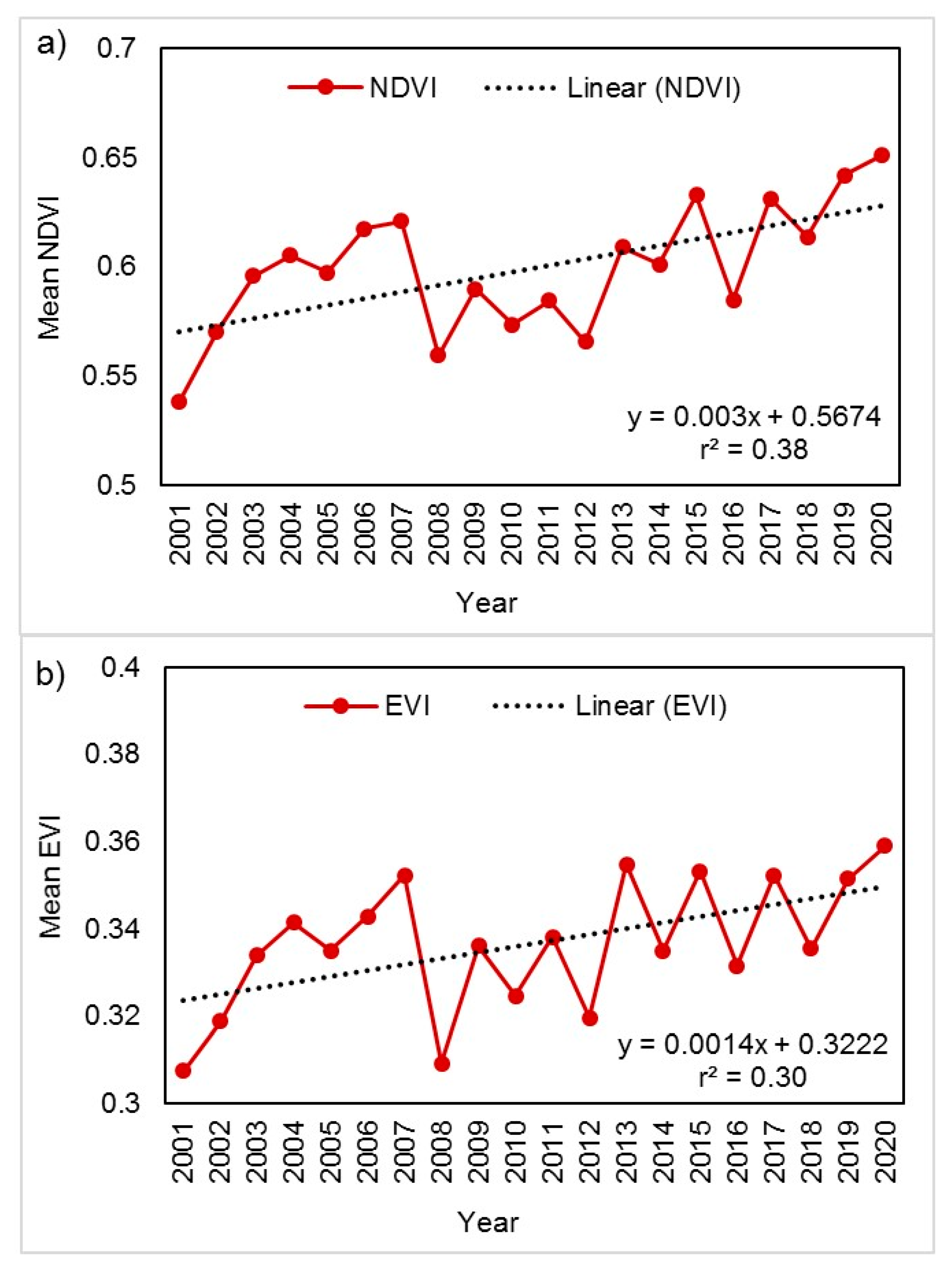
Figure 4 shows the trend of the NDVI and EVI over the last twenty years in the UKR Basin. By averaging the mean NDVI (Figure 4a) and EVI values (Figure 4b) over all pixels within the UKR Basin, the linear regression model was developed to identify the vegetation temporal variation since 2000. The mean NDVI values vary from ~0.54 to 0.64 while the mean EVI has a range of ~0.31 to 0.35. It is observed that there has been an overall temporal increasing trend in NDVI values since 2007. As shown in Figure 4a, the mean NDVI showed a significant greening trend (p < 0.05) with an increasing rate of 0.001/year. This implies that the UKR Basin has experienced an obvious vegetation greening and ecological improvement process since the new millennium. Although the NDVI showed a significant increasing trend, the inter-annual fluctuation is relatively greater, especially from 2009 to 2015. In addition, it is also seen that the mean and standard deviation of the annual NDVI from 2001–2020 were 0.55 and ±0.015, respectively. Unlike the NDVI, the mean EVI showed an insignificant increasing trend over the last twenty years.
4.2.2. Seasonal Variability of NDVI and EVI
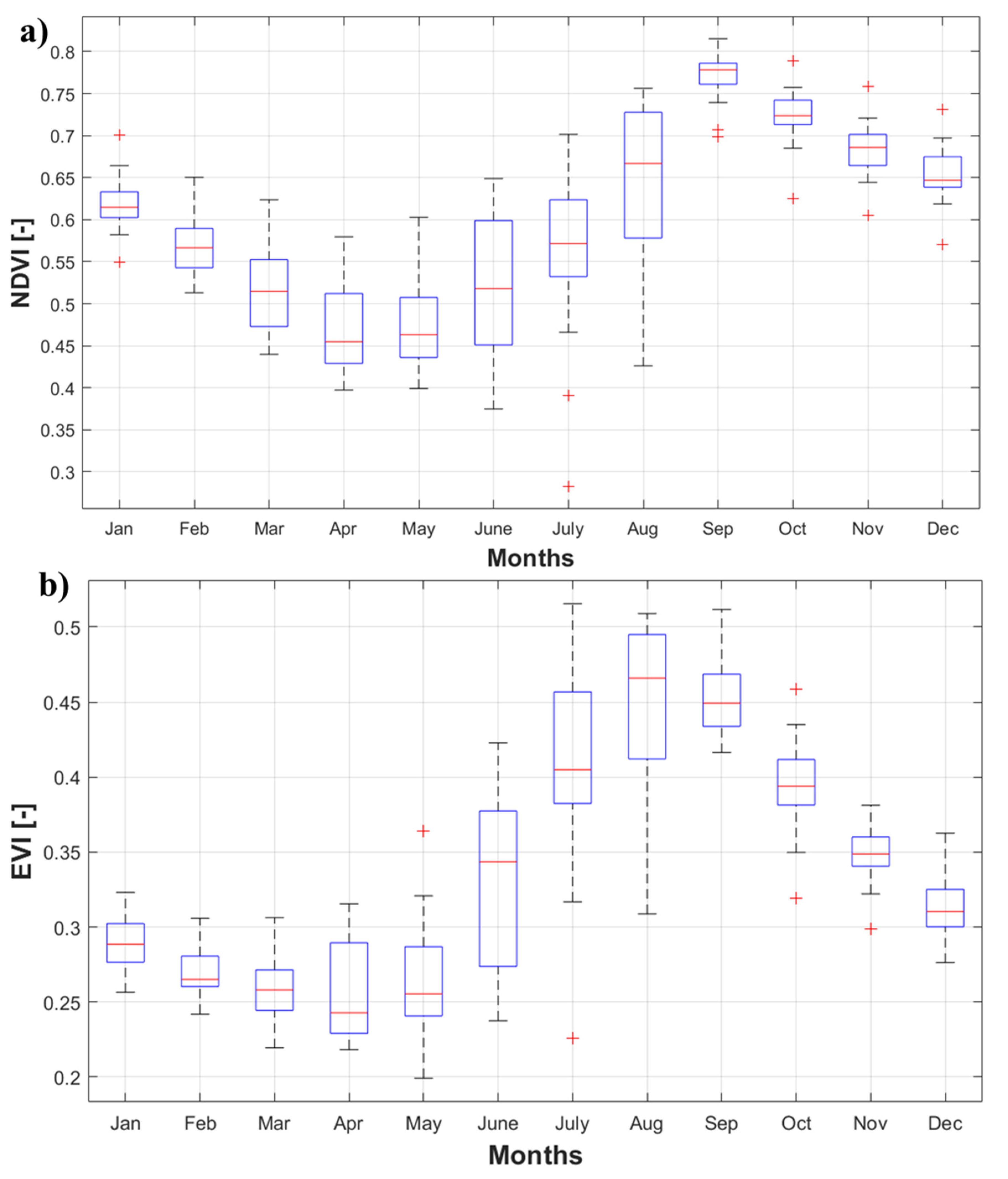
Figure 5 shows the seasonal patterns of the NDVI and EVI for the UKR Basin. The boxplot reflects the mean monthly values of the NDVI (Figure 5a) and EVI (Figure 5b) for the twenty years (2001–2020). It is observed that the NDVI and EVI have their seasonal peak in September and August, respectively, while April is observed to have the lowest NDVI and EVI mean values in the UKR Basin. Further, it can be seen from Figure 5 that monthly NDVI values have fewer fluctuations, especially in the winter season, as compared to the monthly EVI values. It is also observed that the vegetation greening usually starts from May and reaches its maximum in September (NDVI) and August (EVI), and thereafter starts decreasing till the next April. This shows that the seasonality of the EVI and NDVI in the UKR Basin follows a similar pattern.
4.3. Spatial Variations of NDVI and EVI
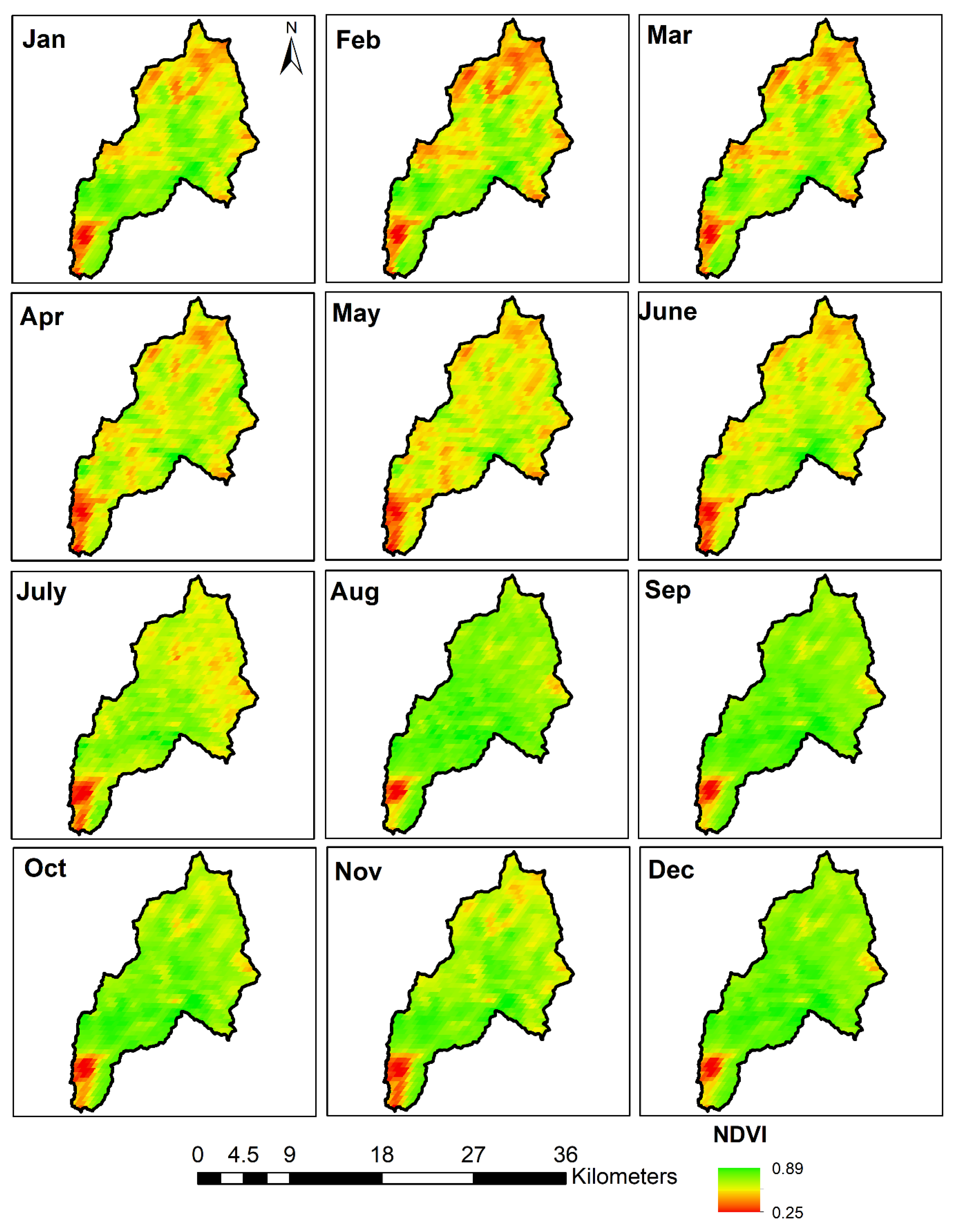
Figure 6 shows the spatial plots of long-term mean monthly NDVI for the period of 2001 to 2020. It can be seen that January to June show a higher variation in the NDVI than July to December, as more variation is observed in NDVI values from January to June than the rest of the year. Further, higher vegetation greenness is seen from July to December. The mean NDVI varies from 0.25 to 0.89. Among all the months, February has a larger number of red pixels covering the UKR Basin, which shows that majority of the basin has lower NDVI values in this month. However, the reverse pattern is seen in the month of December, where the majority of the basin is covered with higher NDVI values. Similar patterns are observed in the spatial analysis of the EVI (Figure 7), however, the range of the mean EVI (0.15–0.65) is smaller than the mean NDVI.
4.4. Relationship of NDVI and EVI with Different Hydroclimatic Factors
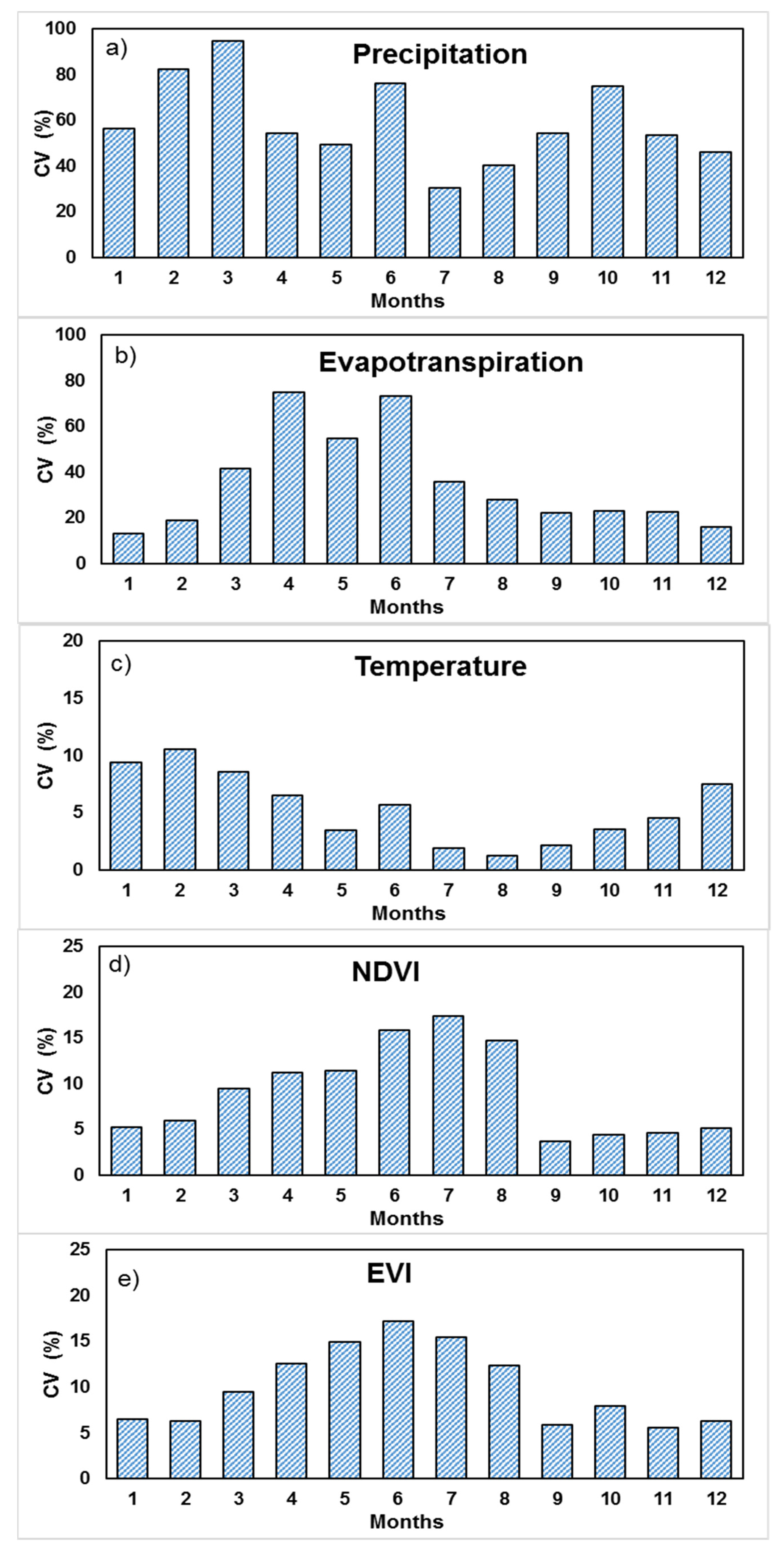
Figure 8 shows the coefficient of variation (CV) of the different hydroclimatic factors as well as the vegetation indices considered in this study. It represents the long-term monthly CV values for precipitation, temperature, ET, NDVI, and EVI. The maximum variation in the CV is observed for the precipitation followed by the ET and temperature. The CV of precipitation increases from ~60% (January), reaching its highest value up to ~95% (March), and then declines sharply with the lowest CV of ~30% (July) (Figure 8a). In general, high seasonal variations are seen in the CV of precipitation in non-monsoon months. Unlike precipitation, the CV of ET increases from ~15% (January), reaching its maximum value of ~80% (April and June), and then it declines for the rest of the year (Figure 8b). The variability of the temperature from July to September is lower (CV = ~2% in August) than the variability in the rest of the year (Figure 8c). Among the vegetation indices, the NDVI and EVI show a similar trend throughout the seasons. The NDVI variations increase from January to July, from ~5% to ~18%, respectively (Figure 8d). Similar patterns were observed in the CV of the EVI as shown in Figure 8e. It is clear from the patterns of the EVI and NDVI that higher variations are observed from May to August that correspond to the different plantation dates and their growth and maturity period and the vegetation type in the catchment.
Figure 9 shows the relationship of the NDVI and EVI with monthly evapotranspiration and precipitation. The EVI is strongly correlated with ET, with r2 = 0.73, whereas the NDVI showed satisfactory performance with r2 = 0.45. On the other hand, the relationship between the EVI and precipitation yielded r2 = 0.34, whereas no relationship was observed between the NDVI and precipitation. Among the two vegetation indices selected here, the EVI showed better correlation between hydrological factors, ET and precipitation. Thus, the EVI can be a better option when selecting the vegetation proxy to determine the biophysical characteristics.
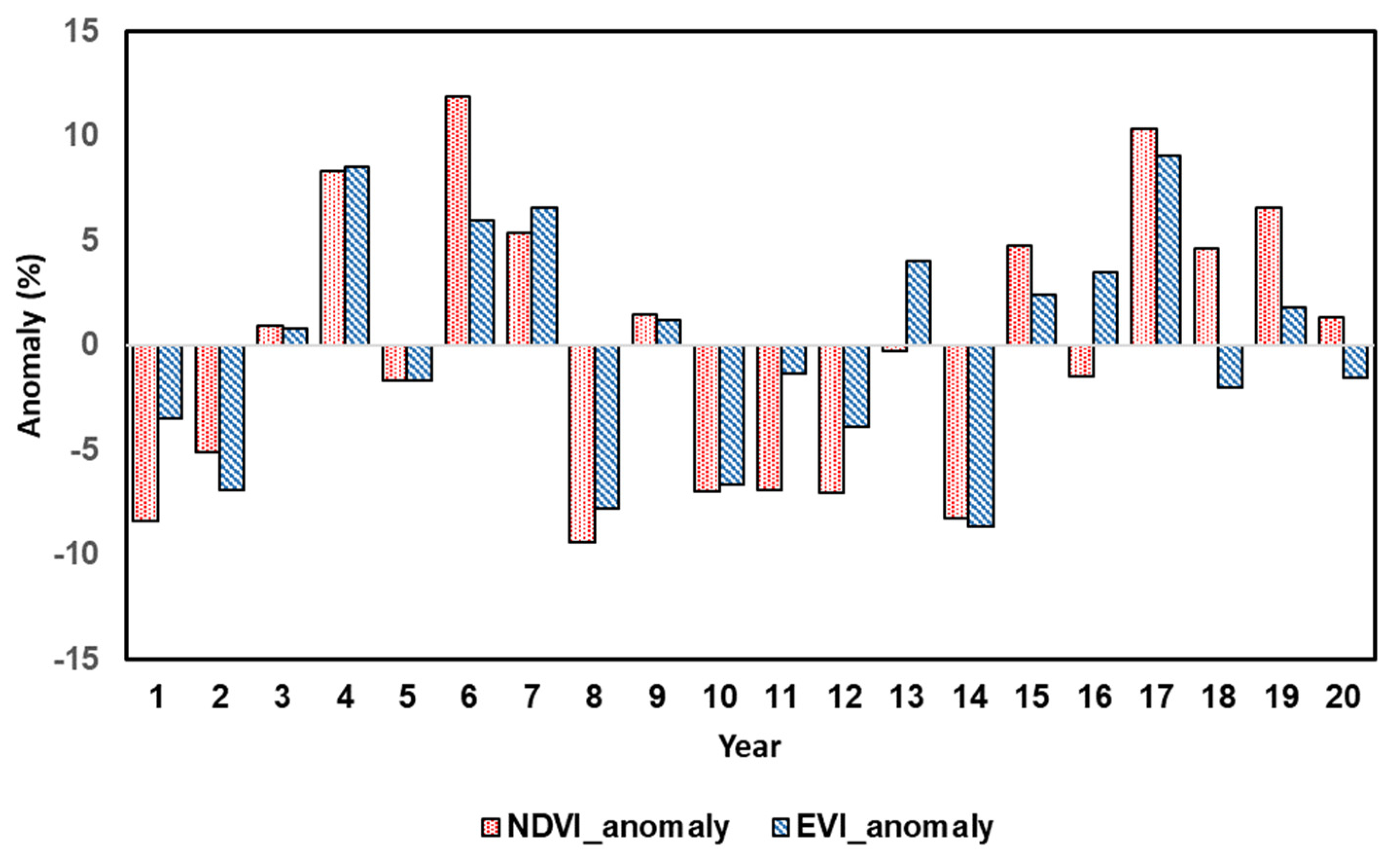
Figure 10 shows the NDVI and EVI anomalies from 2001 to 2020 to show the pattern of drought occurrence in the UKR region. The drought severity ranged from normal to moderate drought conditions. The variation of the NDVI and EVI with a positive value indicates normal conditions (non-drought period), whereas a negative value of anomalies indicates drought conditions based on the range. According to the drought severity range, there existed only mild drought conditions in the UKR Basin. The mild drought conditions in the basin occurred in most of the years and reached a maximum in the year of 2008. It can also be inferred from the figure that almost fifty percent of the years were under normal conditions and the remaining years suffered from mild drought periods. From 2015 to 2020, there were very few drought events.
5. Discussion
The UKR Basin region falls under the lower Himalayan range where the climate is temperate. Under such climatic conditions, it is observed that the basin generally has wetter summers and cooler winters. The maximum amount of precipitation falls in JJAS as observed from Figure 2. This is also consistent with previous studies in the Himalayan region of the Indian sub-continent [3,4]. Further, it is observed that the ET is usually lower than the precipitation (<130 mm) in most of the months of the year throughout the twenty-year period (2001–2020). This shows that the UKR Basin is mostly governed by energy-limited conditions [62,63]. Unlike precipitation (Figure 8a) and ET (Figure 8b), the temperature showed the lowest variation in the last twenty years, though there were seasonal variations (Figure 8c). This may be attributed to the fluctuations in the precipitation and ET over the time period within this region. There was a shift in the vegetation pattern across the lower Himalayan range that altered the feedback mechanisms between climate–vegetation interactions [32,34].
The vegetation greenness over the UKR Basin was investigated using two different vegetation indices, namely, the NDVI and EVI, for the twenty-year period. Both of the vegetation indices showed an increasing trend in the vegetation greening over the given time period. The mean NDVI and EVI increased from 0.54 and 0.31 (2001), respectively, to 0.65 and 0.36 (2020). This shows that the UKR Basin has experienced greater vegetation greening processes over the past two decades. This pattern is supported by the findings of previous studies in similar ecosystems [3,4]. It is noteworthy to mention that the NDVI is consistently higher than EVI values estimated over the UKR Basin from 2001 to 2020. This is due to the fact that the EVI considers the effect of aerosol correction and canopy background adjustments which are not accounted for in the NDVI estimation [46,48,56]. As this catchment falls under a humid region, the canopy layer and the aerosol particles play a critical role in determining biophysical characteristics through any vegetation indices [49,50].
As compared with both the vegetation indices. The EVI seems to correlate with ET and precipitation comparatively better than the NDVI. The EVI is found to perform better than the NDVI and is also consistent with other field- and remote sensing-based findings [64,65]. It is also observed that both the NDVI and EVI have shown up to a one- or two-month lag with the precipitation. These differences in timing by the EVI and NDVI responding to variations in the precipitation in the monsoon season are probably responsible for the lack of a clear linear relationship between vegetation greenness and precipitation. Further, the magnitudes of vegetation phenology (i.e., NDVI and EVI) showed a strong correspondence with the magnitudes of ET (Figure 9a). It is evident from the strong correlation between the EVI and ET that changes in vegetation phenology can be better captured using the EVI, as it is more sensitive in temperate regions. These results are consistent with the findings of previous studies that reported a strong correspondence between the seasonality of satellite-derived vegetation indices (e.g., EVI) and hydroclimatic (e.g., ET) factors [66,67].
6. Conclusions
In the present study, the Himalayan ecosystem is focused on to understand the response of vegetation to different hydroclimatic factors. Vegetation monitoring is an arduous task in the Himalayan regions due to the rugged and complex topography and extremely harsh climatic conditions. Therefore, a remote sensing approach acts as a boon in studying and monitoring vegetation and evaluating its hydrological response in ungauged catchments. In the current study, the UKR Basin region situated in the lower Himalayan ranges is used to understand the long-term spatiotemporal variability of vegetation greenness and associated climatic and hydrological drivers within the Upper Khoh River (UKR) region.
The NDVI and EVI time series data were derived from MODIS using GEE for the period of 2001 to 2020. Thereafter, the recent precipitation, temperature, and ET datasets were utilised to understand the hydroclimatic conditions in the UKR Basin. It is found that both the NDVI and EVI have shown an increasing trend in the vegetation greening over the entire study period, such that the NDVI was consistently higher than the EVI. Strong seasonal control is observed, where a seasonal peak of the NDVI and EVI is found in September and August, respectively. It is evident from the strong correlation between the EVI and ET that changes in vegetation phenology can be better captured using the EVI than the NDVI. In the UKR basin, droughts are always mild, and there has been never a period with any moderate or severe drought, leading to vegetation greenness in the basin. The outcomes of this study can help in ecological environment protection and water resource management in the UKR Basin and other high mountain regions in the Himalayas. Additionally, we can explore the different types of vegetation and the periodic large-scale die-offs of certain plant species in the Himalayas in our future studies.
Author Contributions
N.K. and A.S. conceived the original idea and performed the literature survey, research, data analysis, and result interpretation. N.K. designed and worked on the satellite data interpretation in GEE. N.K. and A.S. prepared the manuscript with contributions from all the co-authors. U.C.D. helped in conceptualising, conducting, editing, and reviewing the manuscript. All authors have read and agreed to the published version of the manuscript.
Funding
This research received no external funding.
Institutional Review Board Statement
Not applicable.
Informed Consent Statement
Not applicable.
Data Availability Statement
Datasets used in this study are publicly available and can be accessed from the online repositories (https://developers.google.com/earth-engine/datasets) as mentioned in the Data and Methods sections.
Acknowledgments
The authors are thankful to the Google Earth Engine team who provided excellent online tutorials and support, which enabled them to carry out this work.
Conflicts of Interest
The authors declare no conflict of interest.
References
- Tiwari, P. Land-use changes in Himalaya and their impact on the plains ecosystem: Need for sustainable land use. Land Use Policy 2000, 17, 101–111. [Google Scholar] [CrossRef]
- Sarkar, S.; Kafatos, M. Interannual variability of vegetation over the Indian sub-continent and its relation to the different meteorological parameters. Remote Sens. Environ. 2004, 90, 268–280. [Google Scholar] [CrossRef]
- Mishra, N.B.; Chaudhuri, G. Spatio-temporal analysis of trends in seasonal vegetation productivity across Uttarakhand, Indian Himalayas, 2000–2014. Appl. Geogr. 2015, 56, 29–41. [Google Scholar] [CrossRef]
- Pandey, R.; Kumar, P.; Archie, K.M.; Gupta, A.K.; Joshi, P.; Valente, D.; Petrosillo, I. Climate change adaptation in the western-Himalayas: Household level perspectives on impacts and barriers. Ecol. Indic. 2018, 84, 27–37. [Google Scholar] [CrossRef]
- Joshi, P.; Rawat, A.; Narula, S.; Sinha, V. Assessing impact of climate change on forest cover type shifts in Western Himalayan Eco-region. J. For. Res. 2012, 23, 75–80. [Google Scholar] [CrossRef]
- Shrestha, U.B.; Gautam, S.; Bawa, K.S. Widespread climate change in the Himalayas and associated changes in local ecosystems. PLoS ONE 2012, 7, e36741. [Google Scholar] [CrossRef]
- Haigh, M.J.; Rawat, J.; Rawat, M.; Bartarya, S.; Rai, S. Interactions between forest and landslide activity along new highways in the Kumaun Himalaya. For. Ecol. Manag. 1995, 78, 173–189. [Google Scholar] [CrossRef]
- Munsi, M.; Areendran, G.; Joshi, P. Modeling spatio-temporal change patterns of forest cover: A case study from the Himalayan foothills (India). Reg. Environ. Chang. 2012, 12, 619–632. [Google Scholar] [CrossRef]
- Batar, A.K.; Watanabe, T.; Kumar, A. Assessment of land-use/land-cover change and forest fragmentation in the Garhwal Himalayan Region of India. Environments 2017, 4, 34. [Google Scholar] [CrossRef]
- Hamid, M.; Khuroo, A.A.; Malik, A.H.; Ahmad, R.; Singh, C.P.; Dolezal, J.; Haq, S.M. Early evidence of shifts in Alpine summit vegetation: A case study from Kashmir Himalaya. Front. Plant Sci. 2020, 11, 421. [Google Scholar] [CrossRef]
- Baldocchi, D.; Falge, E.; Gu, L.; Olson, R.; Hollinger, D.; Running, S.; Anthoni, P.; Bernhofer, C.; Davis, K.; Evans, R. FLUXNET: A new tool to study the temporal and spatial variability of ecosystem-scale carbon dioxide, water vapor, and energy flux densities. Bull. Am. Meteorol. Soc. 2001, 82, 2415–2434. [Google Scholar] [CrossRef]
- Bonan, G. Ecological Climatology: Concepts and Applications; Cambridge University Press: Cambridge, UK, 2015. [Google Scholar]
- Romano, N.; Palladino, M.; Chirico, G. Parameterization of a bucket model for soil-vegetation-atmosphere modeling under seasonal climatic regimes. Hydrol. Earth Syst. Sci. 2011, 15, 3877–3893. [Google Scholar] [CrossRef]
- Srivastava, A.; Rodriguez, J.F.; Saco, P.M.; Kumari, N.; Yetemen, O. Global Analysis of Atmospheric Transmissivity Using Cloud Cover, Aridity and Flux Network Datasets. Remote Sens. 2021, 13, 1716. [Google Scholar] [CrossRef]
- Jackson, T.J.; Chen, D.; Cosh, M.; Li, F.; Anderson, M.; Walthall, C.; Doriaswamy, P.; Hunt, E.R. Vegetation water content mapping using Landsat data derived normalized difference water index for corn and soybeans. Remote Sens. Environ. 2004, 92, 475–482. [Google Scholar] [CrossRef]
- Dumka, U.; Moorthy, K.K.; Kumar, R.; Hegde, P.; Sagar, R.; Pant, P.; Singh, N.; Babu, S.S. Characteristics of aerosol black carbon mass concentration over a high altitude location in the Central Himalayas from multi-year measurements. Atmos. Res. 2010, 96, 510–521. [Google Scholar] [CrossRef]
- Srivastava, A.; Kumari, N.; Maza, M. Hydrological response to agricultural land use heterogeneity using variable infiltration capacity model. Water Resour. Manag. 2020, 34, 3779–3794. [Google Scholar] [CrossRef]
- Kumari, N.; Saco, P.M.; Rodriguez, J.F.; Johnstone, S.A.; Srivastava, A.; Chun, K.P.; Yetemen, O. The Grass Is Not Always Greener on the Other Side: Seasonal Reversal of Vegetation Greenness in Aspect-Driven Semiarid Ecosystems. Geophys. Res. Lett. 2020, 47, e2020GL088918. [Google Scholar] [CrossRef]
- Wagener, T.; Sivapalan, M.; Troch, P.; Woods, R. Catchment classification and hydrologic similarity. Geogr. Compass 2007, 1, 901–931. [Google Scholar] [CrossRef]
- Sharma, A.; Wasko, C.; Lettenmaier, D.P. If precipitation extremes are increasing, why aren’t floods? Water Resour. Res. 2018, 54, 8545–8551. [Google Scholar] [CrossRef]
- Yao, J.; Hu, W.; Chen, Y.; Huo, W.; Zhao, Y.; Mao, W.; Yang, Q. Hydro-climatic changes and their impacts on vegetation in Xinjiang, Central Asia. Sci. Total Environ. 2019, 660, 724–732. [Google Scholar] [CrossRef]
- Kumar, U.; Sahoo, B.; Chatterjee, C.; Raghuwanshi, N.S. Evaluation of simplified surface energy balance index (S-SEBI) method for estimating actual evapotranspiration in Kangsabati reservoir command using landsat 8 imagery. J. Indian Soc. Remote Sens. 2020, 48, 1421–1432. [Google Scholar] [CrossRef]
- Ding, Y.; Xu, J.; Wang, X.; Peng, X.; Cai, H. Spatial and temporal effects of drought on Chinese vegetation under different coverage levels. Sci. Total Environ. 2020, 716, 137166. [Google Scholar] [CrossRef]
- Srivastava, A.; Deb, P.; Kumari, N. Multi-model approach to assess the dynamics of hydrologic components in a tropical ecosystem. Water Resour. Manag. 2020, 34, 327–341. [Google Scholar] [CrossRef]
- Scheffer, M.; Holmgren, M.; Brovkin, V.; Claussen, M. Synergy between small-and large-scale feedbacks of vegetation on the water cycle. Glob. Chang. Biol. 2005, 11, 1003–1012. [Google Scholar] [CrossRef]
- Quillet, A.; Peng, C.; Garneau, M. Toward dynamic global vegetation models for simulating vegetation–climate interactions and feedbacks: Recent developments, limitations, and future challenges. Environ. Rev. 2010, 18, 333–353. [Google Scholar] [CrossRef]
- Reddy, K.S.; Ranjan, M. Solar resource estimation using artificial neural networks and comparison with other correlation models. Energy Convers. Manag. 2003, 44, 2519–2530. [Google Scholar] [CrossRef]
- Zhang, Y.; Gao, J.; Liu, L.; Wang, Z.; Ding, M.; Yang, X. NDVI-based vegetation changes and their responses to climate change from 1982 to 2011: A case study in the Koshi River Basin in the middle Himalayas. Glob. Planet. Chang. 2013, 108, 139–148. [Google Scholar] [CrossRef]
- Adamala, S.; Srivastava, A. Comparative evaluation of daily evapotranspiration using artificial neural network and variable infiltration capacity models. Agric. Eng. Int. CIGR J. 2018, 20, 32–39. [Google Scholar]
- Kumar, S.V.; Holmes, T.; Andela, N.; Dharssi, I.; Hain, C.; Peters-Lidard, C.; Mahanama, S.P.; Arsenault, K.R.; Nie, W.; Getirana, A. The 2019–2020 Australian drought and bushfires altered the partitioning of hydrological fluxes. Geophys. Res. Lett. 2021, 48, e2020GL091411. [Google Scholar] [CrossRef]
- Elbeltagi, A.; Kumari, N.; Dharpure, J.K.; Mokhtar, A.; Alsafadi, K.; Kumar, M.; Mehdinejadiani, B.; Ramezani Etedali, H.; Brouziyne, Y.; Islam, T. Prediction of combined terrestrial evapotranspiration index (CTEI) over large river basin based on machine learning approaches. Water 2021, 13, 547. [Google Scholar] [CrossRef]
- Nemani, R.R.; Keeling, C.D.; Hashimoto, H.; Jolly, W.M.; Piper, S.C.; Tucker, C.J.; Myneni, R.B.; Running, S.W. Climate-driven increases in global terrestrial net primary production from 1982 to 1999. Science 2003, 300, 1560–1563. [Google Scholar] [CrossRef] [PubMed]
- Srivastava, A.; Sahoo, B.; Raghuwanshi, N.S.; Singh, R. Evaluation of variable-infiltration capacity model and MODIS-terra satellite-derived grid-scale evapotranspiration estimates in a River Basin with Tropical Monsoon-Type climatology. J. Irrig. Drain. Eng. 2017, 143, 04017028. [Google Scholar] [CrossRef]
- Papagiannopoulou, C.; Miralles, D.; Dorigo, W.A.; Verhoest, N.; Depoorter, M.; Waegeman, W. Vegetation anomalies caused by antecedent precipitation in most of the world. Environ. Res. Lett. 2017, 12, 074016. [Google Scholar] [CrossRef]
- Srivastava, A.; Saco, P.M.; Rodriguez, J.F.; Kumari, N.; Chun, K.P.; Yetemen, O. The role of landscape morphology on soil moisture variability in semi-arid ecosystems. Hydrol. Process. 2021, 35, e13990. [Google Scholar] [CrossRef]
- Srivastava, A.; Sahoo, B.; Raghuwanshi, N.S.; Chatterjee, C. Modelling the dynamics of evapotranspiration using Variable Infiltration Capacity model and regionally calibrated Hargreaves approach. Irrig. Sci. 2018, 36, 289–300. [Google Scholar] [CrossRef]
- Piao, S.; Wang, X.; Park, T.; Chen, C.; Lian, X.; He, Y.; Bjerke, J.W.; Chen, A.; Ciais, P.; Tømmervik, H. Characteristics, drivers and feedbacks of global greening. Nat. Rev. Earth Environ. 2020, 1, 14–27. [Google Scholar] [CrossRef]
- Mukherji, A.; Molden, D.; Nepal, S.; Rasul, G.; Wagnon, P. Himalayan waters at the crossroads: Issues and challenges. Int. J. Water Resour. Dev. 2015, 31, 151–160. [Google Scholar] [CrossRef]
- Devanand, A.; Huang, M.; Ashfaq, M.; Barik, B.; Ghosh, S. Choice of irrigation water management practice affects indian summer monsoon rainfall and its extremes. Geophys. Res. Lett. 2019, 46, 9126–9135. [Google Scholar] [CrossRef]
- Dumka, U.; Ningombam, S.S.; Kaskaoutis, D.; Madhavan, B.; Song, H.-J.; Angchuk, D.; Jorphail, S. Long-term (2008–2018) aerosol properties and radiative effect at high-altitude sites over western trans-Himalayas. Sci. Total Environ. 2020, 734, 139354. [Google Scholar] [CrossRef]
- Kumari, N.; Srivastava, A. An approach for estimation of evapotranspiration by standardizing parsimonious method. Agric. Res. 2020, 9, 301–309. [Google Scholar] [CrossRef]
- Maza, M.; Srivastava, A.; Bisht, D.S.; Raghuwanshi, N.S.; Bandyopadhyay, A.; Chatterjee, C.; Bhadra, A. Simulating hydrological response of a monsoon dominated reservoir catchment and command with heterogeneous cropping pattern using VIC model. J. Earth Syst. Sci. 2020, 129, 1–16. [Google Scholar] [CrossRef]
- Elbeltagi, A.; Aslam, M.R.; Malik, A.; Mehdinejadiani, B.; Srivastava, A.; Bhatia, A.S.; Deng, J. The impact of climate changes on the water footprint of wheat and maize production in the Nile Delta, Egypt. Sci. Total Environ. 2020, 743, 140770. [Google Scholar] [CrossRef] [PubMed]
- Srivastava, A.; Yetemen, O.; Kumari, N.; Saco, P. Aspect-controlled spatial and temporal soil moisture patterns across three different latitudes. In Proceedings of the 23rd International Congress on Modeling and Simulation (MODSIM2019), Canberra, Australia, 1–6 December 2019; pp. 979–985. [Google Scholar]
- Huete, A.; Justice, C.; Van Leeuwen, W. MODIS vegetation index (MOD13). Algorithm Theor. Basis Doc. 1999, 3, 295–309. [Google Scholar]
- Matsushita, B.; Yang, W.; Chen, J.; Onda, Y.; Qiu, G. Sensitivity of the enhanced vegetation index (EVI) and normalized difference vegetation index (NDVI) to topographic effects: A case study in high-density cypress forest. Sensors 2007, 7, 2636–2651. [Google Scholar] [CrossRef]
- Gao, X.; Huete, A.R.; Ni, W.; Miura, T. Optical–biophysical relationships of vegetation spectra without background contamination. Remote Sens. Environ. 2000, 74, 609–620. [Google Scholar] [CrossRef]
- Huete, A.; Didan, K.; Miura, T.; Rodriguez, E.P.; Gao, X.; Ferreira, L.G. Overview of the radiometric and biophysical performance of the MODIS vegetation indices. Remote Sens. Environ. 2002, 83, 195–213. [Google Scholar] [CrossRef]
- Wardlow, B.D.; Egbert, S.L.; Kastens, J.H. Analysis of time-series MODIS 250 m vegetation index data for crop classification in the US Central Great Plains. Remote Sens. Environ. 2007, 108, 290–310. [Google Scholar] [CrossRef]
- Yan, E.; Wang, G.; Lin, H.; Xia, C.; Sun, H. Phenology-based classification of vegetation cover types in Northeast China using MODIS NDVI and EVI time series. Int. J. Remote Sens. 2015, 36, 489–512. [Google Scholar] [CrossRef]
- Lee, K.H. Constructing a non-linear relationship between the incoming solar radiation and bright sunshine duration. Int. J. Climatol. 2010, 30, 1884–1892. [Google Scholar] [CrossRef]
- Kumar, R. Western Himalaya Basement Reactivation. In Basement Tectonics 7; Springer: Dordrecht, The Netherlands, 1992; pp. 95–110. [Google Scholar]
- Huffman, G.J.; Bolvin, D.T.; Braithwaite, D.; Hsu, K.; Joyce, R.; Xie, P.; Yoo, S.-H. NASA global precipitation measurement (GPM) integrated multi-satellite retrievals for GPM (IMERG). Algorithm Theor. Basis Doc. (ATBD) Version 2015, 4, 26. [Google Scholar]
- Wan, Z. Collection-5 MODIS Land Surface Temperature Products Users’ Guide; ICESS, University of California: Santa Barbara, CA, USA, 2007. [Google Scholar]
- Mu, Q.; Heinsch, F.A.; Zhao, M.; Running, S.W. Development of a global evapotranspiration algorithm based on MODIS and global meteorology data. Remote Sens. Environ. 2007, 111, 519–536. [Google Scholar] [CrossRef]
- Mu, Q.; Zhao, M.; Running, S.W. Improvements to a MODIS global terrestrial evapotranspiration algorithm. Remote Sens. Environ. 2011, 115, 1781–1800. [Google Scholar] [CrossRef]
- Farr, T.G.; Rosen, P.A.; Caro, E.; Crippen, R.; Duren, R.; Hensley, S.; Kobrick, M.; Paller, M.; Rodriguez, E.; Roth, L. The shuttle radar topography mission. Rev. Geophys. 2007, 45. [Google Scholar] [CrossRef]
- Rouse, J.W.; Haas, R.H.; Schell, J.A.; Deering, D.W.; Harlan, J.C. Monitoring the vernal advancement and retrogradation (green wave effect) of natural vegetation. NASA/GSFC Type III Final Rep. Greenbelt Md 1974, 371. [Google Scholar]
- Kumari, N.; Yetemen, O.; Srivastava, A.; Rodriguez, J.F.; Saco, P.M. The spatio-temporal NDVI analysis for two different Australian catchments. In Proceedings of the 23rd International Congress on Modeling and Simulation (MODSIM2019), Canberra, Australia, 1–6 December 2019; pp. 958–964. [Google Scholar]
- Gorelick, N.; Hancher, M.; Dixon, M.; Ilyushchenko, S.; Thau, D.; Moore, R. Google Earth Engine: Planetary-scale geospatial analysis for everyone. Remote Sens. Environ. 2017, 202, 18–27. [Google Scholar] [CrossRef]
- Vaani, N.; Porchelvan, P. Assessment of long term agricultural drought in Tamilnadu, India using NDVI anomaly. Dis. Adv 2017, 10, 1–10. [Google Scholar]
- Budyko, M.I. Climate and Life; Academic: San Diego, CA, USA, 1974. [Google Scholar]
- Zhang, L.; Dawes, W.; Walker, G. Response of mean annual evapotranspiration to vegetation changes at catchment scale. Water Resour. Res. 2001, 37, 701–708. [Google Scholar] [CrossRef]
- White, K.; Pontius, J.; Schaberg, P. Remote sensing of spring phenology in northeastern forests: A comparison of methods, field metrics and sources of uncertainty. Remote Sens. Environ. 2014, 148, 97–107. [Google Scholar] [CrossRef]
- Karkauskaite, P.; Tagesson, T.; Fensholt, R. Evaluation of the plant phenology index (PPI), NDVI and EVI for start-of-season trend analysis of the Northern Hemisphere boreal zone. Remote Sens. 2017, 9, 485. [Google Scholar] [CrossRef]
- Wagle, P.; Gowda, P.H.; Northup, B.K.; Starks, P.J.; Neel, J.P. Response of tallgrass prairie to management in the US Southern Great Plains: Site descriptions, management practices, and eddy covariance instrumentation for a long-term experiment. Remote Sens. 2019, 11, 1988. [Google Scholar] [CrossRef]
- Wagle, P.; Xiao, X.; Torn, M.S.; Cook, D.R.; Matamala, R.; Fischer, M.L.; Jin, C.; Dong, J.; Biradar, C. Sensitivity of vegetation indices and gross primary production of tallgrass prairie to severe drought. Remote Sens. Environ. 2014, 152, 1–14. [Google Scholar] [CrossRef]
Figure 1.
(a) The location map of the study area within India; (b) the index map of Upper Khoh River (UKR) Basin in Uttarakhand, India as an elevation map.
Figure 1.
(a) The location map of the study area within India; (b) the index map of Upper Khoh River (UKR) Basin in Uttarakhand, India as an elevation map.

Figure 2.
Inter-annual variability of precipitation (PPT) in mm, temperature in °C, and evapotranspiration (ET) in mm over twenty years (2001–2020) for the UKR Basin. Note that 1–12 on the x-axis represent the months from January to December.
Figure 2.
Inter-annual variability of precipitation (PPT) in mm, temperature in °C, and evapotranspiration (ET) in mm over twenty years (2001–2020) for the UKR Basin. Note that 1–12 on the x-axis represent the months from January to December.
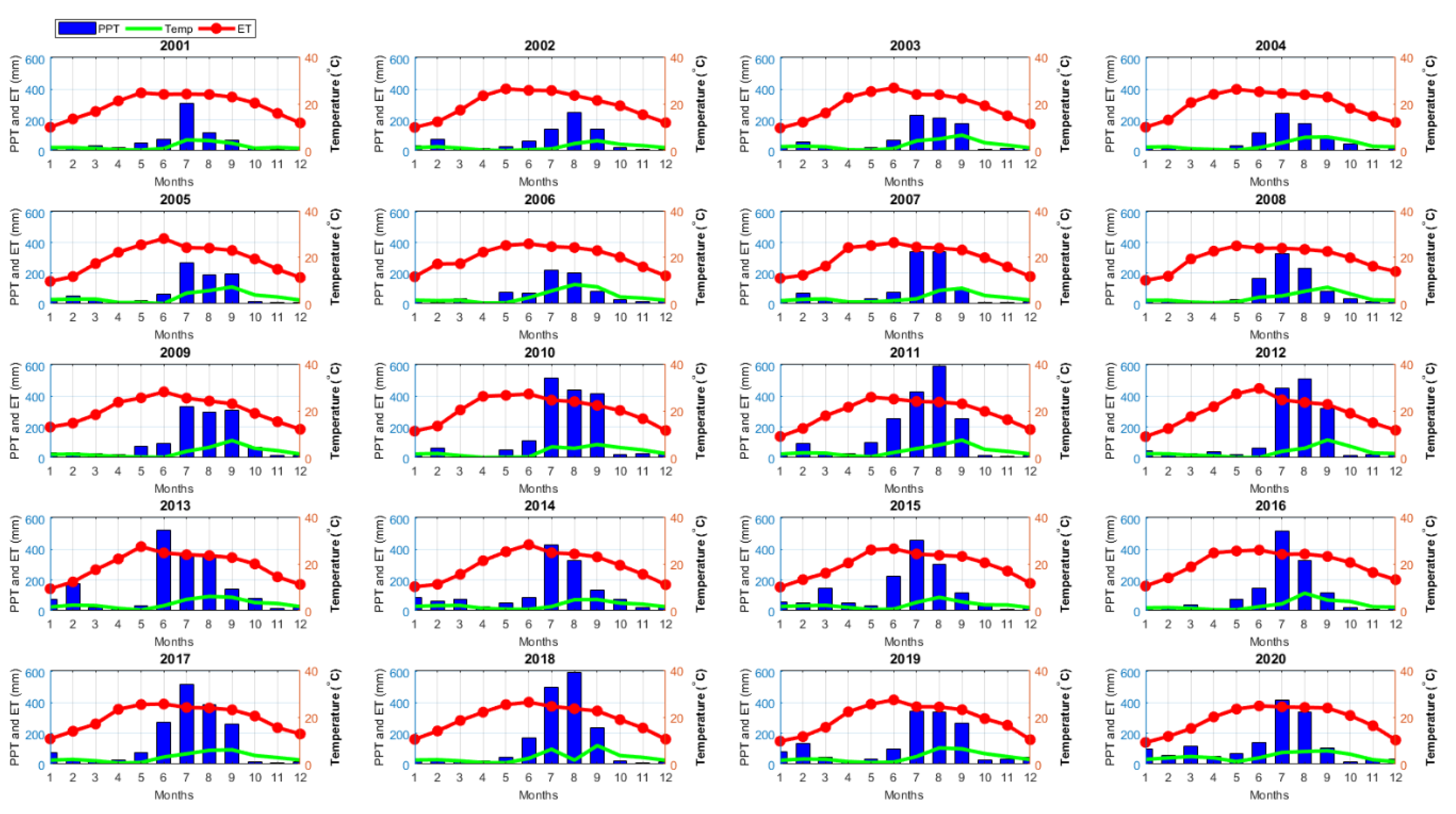
Figure 3.
Boxplot for the inter-annual variability of (a) NDVI and (b) EVI over twenty years (2001–2020) for the UKR Basin.
Figure 3.
Boxplot for the inter-annual variability of (a) NDVI and (b) EVI over twenty years (2001–2020) for the UKR Basin.

Figure 4.
Inter-annual variability of (a) NDVI and (b) EVI over the twenty-year period (2001–2020) for the UKR Basin.
Figure 4.
Inter-annual variability of (a) NDVI and (b) EVI over the twenty-year period (2001–2020) for the UKR Basin.

Figure 5.
Mean monthly temporal variations of (a) NDVI and (b) EVI over the twenty-year period (2001–2020) for the UKR Basin.
Figure 5.
Mean monthly temporal variations of (a) NDVI and (b) EVI over the twenty-year period (2001–2020) for the UKR Basin.

Figure 6.
Mean monthly spatial variations of NDVI for the twenty-year period (2001–2020) for the UKR Basin.
Figure 6.
Mean monthly spatial variations of NDVI for the twenty-year period (2001–2020) for the UKR Basin.

Figure 7.
Mean monthly spatial variations of EVI for the twenty-year period (2001–2020) for the UKR Basin.
Figure 7.
Mean monthly spatial variations of EVI for the twenty-year period (2001–2020) for the UKR Basin.
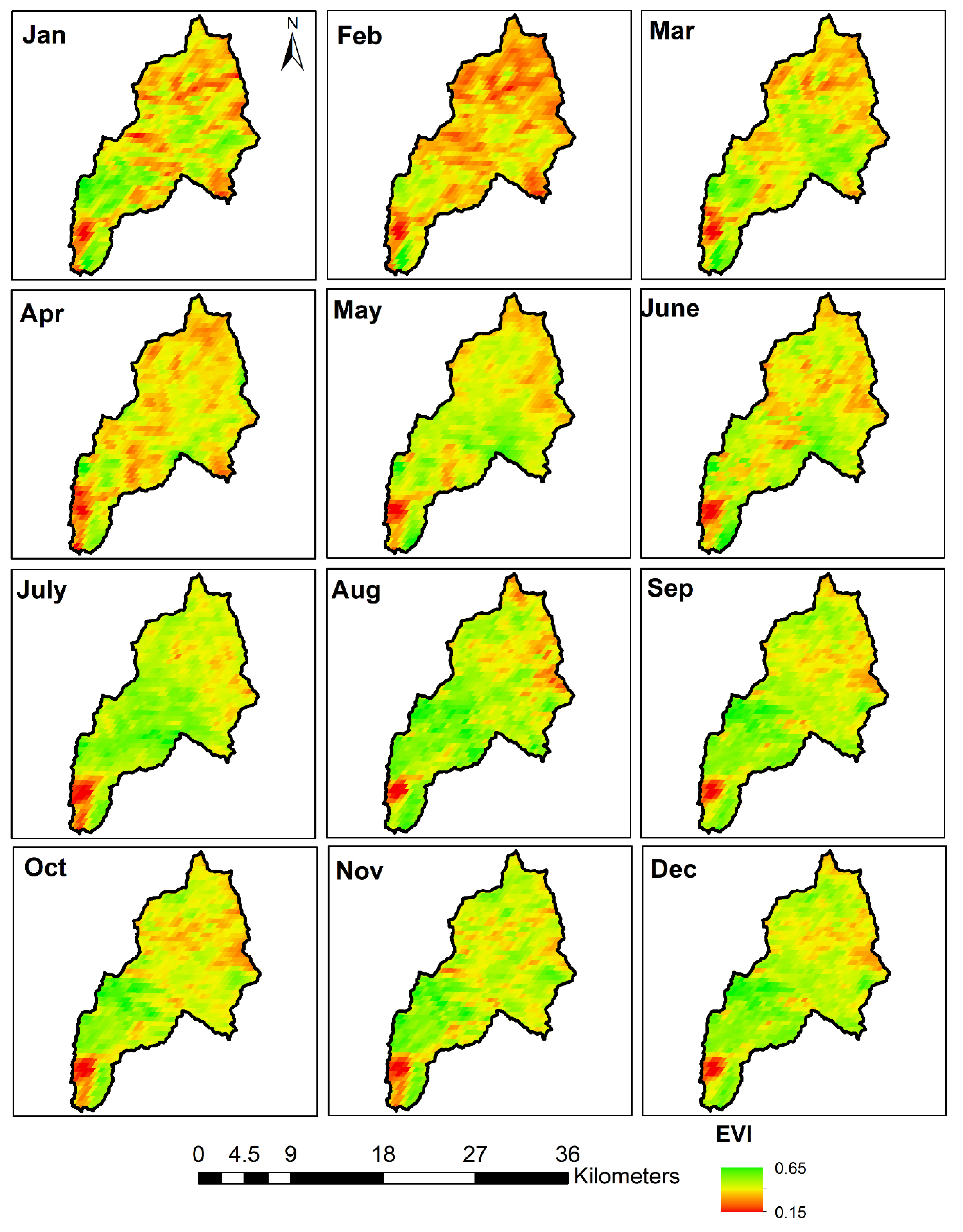
Figure 8.
Mean temporal coefficient of variation (CV in %) plotted as a function of time (months) for (a) precipitation, (b) evapotranspiration, (c) temperature, (d) NDVI for the UKR Basin and (e) EVI. Note that 1–12 on the x-axis represent the months from January to December.
Figure 8.
Mean temporal coefficient of variation (CV in %) plotted as a function of time (months) for (a) precipitation, (b) evapotranspiration, (c) temperature, (d) NDVI for the UKR Basin and (e) EVI. Note that 1–12 on the x-axis represent the months from January to December.

Figure 9.
Relationship of mean temporal EVI plotted as a function of (a) evapotranspiration, (b) precipitation, and mean temporal NDVI plotted as a function of (c) evapotranspiration, (d) precipitation.
Figure 9.
Relationship of mean temporal EVI plotted as a function of (a) evapotranspiration, (b) precipitation, and mean temporal NDVI plotted as a function of (c) evapotranspiration, (d) precipitation.

Figure 10.
NDVI and EVI anomalies shown for the period of 2001–2020 in the UKR Basin. Note that 1 to 20 on the x-axis represent the years from 2001–2020 considered in this study.
Figure 10.
NDVI and EVI anomalies shown for the period of 2001–2020 in the UKR Basin. Note that 1 to 20 on the x-axis represent the years from 2001–2020 considered in this study.

Publisher’s Note: MDPI stays neutral with regard to jurisdictional claims in published maps and institutional affiliations. |
© 2021 by the authors. Licensee MDPI, Basel, Switzerland. This article is an open access article distributed under the terms and conditions of the Creative Commons Attribution (CC BY) license (https://creativecommons.org/licenses/by/4.0/).
Share and Cite
MDPI and ACS Style
Kumari, N.; Srivastava, A.; Dumka, U.C. A Long-Term Spatiotemporal Analysis of Vegetation Greenness over the Himalayan Region Using Google Earth Engine. Climate 2021, 9, 109. https://0-doi-org.brum.beds.ac.uk/10.3390/cli9070109
AMA Style
Kumari N, Srivastava A, Dumka UC. A Long-Term Spatiotemporal Analysis of Vegetation Greenness over the Himalayan Region Using Google Earth Engine. Climate. 2021; 9(7):109. https://0-doi-org.brum.beds.ac.uk/10.3390/cli9070109
Chicago/Turabian StyleKumari, Nikul, Ankur Srivastava, and Umesh Chandra Dumka. 2021. "A Long-Term Spatiotemporal Analysis of Vegetation Greenness over the Himalayan Region Using Google Earth Engine" Climate 9, no. 7: 109. https://0-doi-org.brum.beds.ac.uk/10.3390/cli9070109
Note that from the first issue of 2016, this journal uses article numbers instead of page numbers. See further details here.