
Observed Daily Temperature Variability and Extremes over Southeastern USA (1978–2017)
by
 , and
, and
Souleymane Fall
1,* ,
,
Kapo M. Coulibaly
2, 
Joseph E. Quansah
1,
Gamal El Afandi
1 and
and
Ramble Ankumah
1 1
Department of Agricultural & Environmental Sciences, Tuskegee University, Tuskegee, AL 36088, USA
2
Wood Environmental and Infrastructure Solutions, Costa Mesa, CA 92626, USA
*
Author to whom correspondence should be addressed.
Climate 2021, 9(7), 110; https://0-doi-org.brum.beds.ac.uk/10.3390/cli9070110
Submission received: 19 May 2021
/
Revised: 14 June 2021
/
Accepted: 28 June 2021
/
Published: 1 July 2021
(This article belongs to the Special Issue Modelling and Forecasting Extreme Climate Events)
Abstract
:This study presents an analysis of extreme temperature events over southeastern USA from 1978 to 2017. This region is part of the so-called ‘warming hole’ where long-term surface temperature trends are negative or non-significant, in contrast with the remainder of the country. This study examines whether this distinctive characteristic reflects on the region’s trends in temperature extremes. Daily maximum and minimum temperatures from the US Historical Climatology Network were used to compute extreme indices recommended by the Expert Team on Climate Change Detection and Indices. Temperature extreme indices computed for all stations using the RClimDex package were gridded onto a regular latitude–longitude grid, and a spatiotemporal analysis of associated trends was performed. The results point to a tendency toward warming due to increasing trends in the annual occurrence of the hottest day, the warmest night, warm days, warm nights, summer days, tropical nights, and warm spells, as well as decreases in cool nights, cool days, and frost days. Statistically significant trend changes over large portions of the Southeast were dominated by increases in the frequency of the coldest night, summer days, and warm nights, and decreases in cool nights and frost days. Comparison of our results with other global and regional studies indicate that most of the extreme temperature changes over the Southeast are consistent with findings from other parts of the United States (US) and the world. Overall, this study shows that being part of the ‘warming hole’ does not preclude southeastern US from an intensification of temperature extremes, whether it is an increase in warm extremes or a decrease in cold ones. Further, the results suggest that, should the current trends continue in the long term, the Southeast will not be considered as being part of a warming hole anymore.
1. Introduction
Over the past decades, the frequency and intensity of extreme weather and climate events have been increasing worldwide and now constitute one of the most prominent aspects of climate change [1]. In the United States, this upward trend has been reported in several studies [2,3,4]. According to the World Meteorological Organization [5], from 1970 to 2012, 8835 weather-related disasters including floods, droughts, heatwaves, tropical cyclones, storm surges, and windstorms have caused 1.94 million deaths and have resulted in economic losses of US $2.4 trillion. Overall, the devastating effects of increasingly frequent climate extremes are economic, social, and environmental [6,7,8,9,10]. In fact, extreme weather or climate events affect human and natural systems much more than the average climate by modifying resilience, coping capacity, and adaptive capacity [11,12,13,14]. As a result, there has been a sharp increase in the demand for information services on weather and climate extremes, and the growing attention given to extremes is attested by a large body of studies that has expanded considerably during the recent decades.
Following a first workshop on weather and climate extremes held in 1997 to assess the needs for extreme weather monitoring [15], and relatively early studies on climate extremes [16,17,18,19], an international collaboration was led by the Expert Team on Climate Change Detection and Indices (ETCCDI), based on a two-pronged approach well described by Peterson and Manton [20]. First, the development of 27 climate extreme indices computed from daily precipitation, maximum and minimum temperatures; using the same climate extremes definitions allowed researchers to compare the results from different regions in a consistent manner and to obtain a coherent picture of changes in extremes that are occurring around the world [21]. Second, the organization of regional workshops targeting regions of the world where data are sparse allowed to fill the gaps, perform quality control on the collected data, and compute extreme indices [22]. The workshops, which spanned the 1998–2008 period, resulted in several publications [23,24,25,26,27,28].
A large number of studies have reported observed changes in temperature extremes on a global scale, in particular since 1950. In brief, over land there has generally been (i) a significant increase in hot days, warm nights, warm spell duration, tropical nights, and summer days; (ii) a lengthening of the growing season; (iii) a decrease in cold days and nights, cold spell duration, frost days, and ice days; and (iv) a significant downward trend in diurnal temperature range and extreme temperature range [1,11,29,30,31,32,33,34]. Trends in temperature extremes pointing to a warmer climate are widespread. For example, Aguilar et al. found that, in Central America and northern South America, increases in extremely high temperatures are occurring at a much faster rate than decreases in extremely cold temperatures, thus causing an increase in a diurnal temperature range [26]. Similar trends in temperature extremes were observed by Klen Tank et al. in central and south Asia [27]. Alexander and Arblaster noted a dramatic shift toward warming, especially a significant increase in the number of warm nights and heat waves over Australia [30]. Caesar et al. [28] found increases (decreases) in warm (cold) temperature extremes in the Indo-Pacific region, with warm nights displaying spatially coherent patterns. Similarly, studies conducted on a global scale confirm that significant changes in temperature extremes consistent with a warming climate are occurring over large parts of the world, in particular for indices computed from daily minimum temperatures [29,31].
This overall pattern toward more frequent hot days and nights and fewer cold days and nights is not uniform; a few regions have been found to depart from it, including southeastern USA, which is our study area. For example, trend distribution maps from Alexander et al. [29] indicate that warm days decreased over the Southeast during the second half of the 20th century. The same study points to a decrease in summer days and warm spells. Similarly, Donat et al. [31] found a decrease in warm nights and days over the region during the 1901–2010 period. Decreases in the number of frost days are also found to be much more (less) pronounced in the western (eastern) USA [35]. This pattern is consistent with the negative trends in mean temperature observed over the Southeast in several studies, leading to the term ‘warming hole’ [36,37,38,39,40]. This region has exhibited a discontinuous cooling trend during the 20th century [41,42,43], in contrast with the warming trend across most of the United States. Several causes of the ‘warming hole’ have been identified. Pan et al. [36] attribute this anomaly to changes in low-level circulations that regulate moisture flow and summertime precipitation in the ‘warming hole’ region. As a result, seasonal increases in soil moisture and late-summer evapotranspiration reduce daytime maximum temperatures. Low-level moisture convergence in that region during the summer is also mentioned as a possible cause by Meehl et al. [38], along with cold air advection into the Southeast during the winter season. Other causes of the ‘warming hole’ include the effects of anthropogenic aerosols, land use change, internal climate variability, and various hydrological processes that may be linked to Atlantic and Pacific Sea surface temperatures [37,39,40,44].
The rationale for choosing the Southeast as the study area is to investigate whether this distinctive characteristic (being part of the ‘warming hole’) reflects on the region’s trends in temperature extremes. Therefore, in this study, we use recent observations of daily temperature data to examine temperature variability and further analyze the changes in trends of daily climate extremes of temperature in southeastern USA over 40 years (1978–2017). All climate extreme indices are analyzed at annual time scales only, including monthly ones.
2. Materials and Methods
2.1. Data
The importance of using high-quality and homogeneous daily data when computing climate extremes has been stressed in several studies [45,46,47]. Long-term station records are often affected by inhomogeneities caused by non-climatic factors such as historical changes in observation practices (e.g., change in time of observation), instrumentation, or station location and associated changes in sun exposure and surrounding land use/cover [48,49,50,51]. Such inhomogeneities often result in artificial trends and discontinuities in long-term time series and can yield erroneous characterization of historical climate variations [52]. Removing inhomogeneities from climate records is particularly important when it comes to computing climate extremes because they can result in the validation of false extremes or the characterization of real extremes as outliers or suspect values [47].
The maximum and minimum temperature data used in this study consist of daily observations from the US Historical Climatology Network (USHCN, version 2.5.5) [53,54], and cover a period from 1978 to 2017. The USHCN is a subset of the National Oceanic and Atmospheric Administration (NOAA) Cooperative Observer Program (COOP) network. The criteria for selecting USHCN stations include data completeness, record length, regional and spatial representativity, and historical stability [53]. Over time, previous versions of the USHCN dataset have been considerably improved thanks to extensive quality control procedures and adjustments that account for non-climatic factors which introduce biases in the temperature records [55,56]. More specifically, a wide range of quality assurance checks was performed on the daily data, including simultaneous zeros, duplication of data, impossible values, runs of the same values over a long period, climatological outliers, and various types of inconsistencies. Homogenization procedures included the removal of biases caused by changes in time of observation, station location, instrumentation, and also by urbanization and non-standard siting. Adjustment methods are described in detail by Menne et al. [53] and Menne and Williams [57]. The stations used in this study are shown in Figure 1. Although they mostly consist of USHCN stations, they were supplemented by a few COOP stations to ensure a better coverage at the edges of the study area.
Additional quality control provided by the RClimDex package [58,59] consists of routines including, but not limited to, duplicate dates control, out-of-range values based on fixed threshold values, outliers based on interquartile range exceedance, coherence between maximum and minimum temperatures (Tmax > Tmin), consecutive equal values control, and interdiurnal differences based on fixed threshold values. These routines are part of the EXTRAQC package integrated into the RClimDex program [60]. These quality control procedures allowed the correction and/or removal of unreasonable data values, such as minimum temperatures larger than maximum temperature values, identification of statistical outliers, and their verification against values of close neighboring stations.
The spatial data used in this study originate from the Environmental Systems Research Institute (ESRI) and consist of a shapefile of US states. A subset of southeastern US states was created from the original shapefile. Geographic coordinates of USHCN stations obtained from NOAA were used to create a shapefile of the climate stations.
2.2. Methods
2.2.1. Indices
Twelve indices derived from daily maximum and minimum temperature were used in this study (Table 1). They constitute a subset of sixteen temperature indices recommended by the ETCCDI. The indices, which represent the tails of temperature distribution [46], were calculated using the RClimDex standard software package [58,59]. The subset of temperature indices used in this study can be divided into four groups [29]:
- Percentile-based temperature indices were calculated for the climatological base period 1961–1990 and include the cool nights (TN10p), warm nights (TN90p), cool days (TX10p), and warm days (TX90p);
- Absolute indices consist of monthly values indicating the hottest day (TXx), coldest night (TNn), coldest day (TXn), and warmest night (TNx);
- Threshold indices consist of summer days (SU25), tropical nights (TR20), frost days (FD0), and ice days (ID0);
- Duration indices include warm spell duration indicator (WSDI), and cold spell duration indicator (CSDI).
2.2.2. Analysis Procedures
Before any statistical analysis, indices computed for all stations using the RClimDex package were gridded onto a latitude–longitude grid regularly spaced at 0.2 decimal degrees. The gridding was performed using the Multilevel B-Splines Approximation (MBA) method, which provides functions to interpolate scattered data points. The MBA interpolation algorithm efficiently minimizes the local approximation error for each control point, and the resulting estimate is further refined through a sequence of functions from coarsest to finest levels. MBA has proven to be effective for a high-fidelity reconstruction from sparse and irregularly distributed samples. A detailed description of the specific MBA algorithm used for this study is provided by Lee et al. [63].
The time series for Tmax, Tmin, and indices were created by spatially averaging annual values over the study area as anomalies relative to the study period and by applying cosine weighting. A smooth curve was fitted to the time series using LOESS smoothing [64].
Trends were calculated using Sen’s non-parametric estimator of slope [65], and the significance of the trend was estimated at the 5% level using the Mann–Kendall test [66]. This trend calculation method has been extensively used in similar studies [25,26,28,31], and is suitable for dealing with outliers and non-normal distribution of the data (given that climate indices do not always have a Gaussian distribution).
Once grids for indices were created in the NetCDF format, trends and associated P-values were computed in R and exported to text files which provide, for each grid point, the x,y coordinates and trend analysis values. The text files were loaded into Geographic Information Systems (GIS) software (ArcMap, from ESRI) and used to create corresponding shapefiles. Query expressions were used to find grid points with statistically significant positive and negative trends.
3. Results
3.1. Temperature Trends and Variability
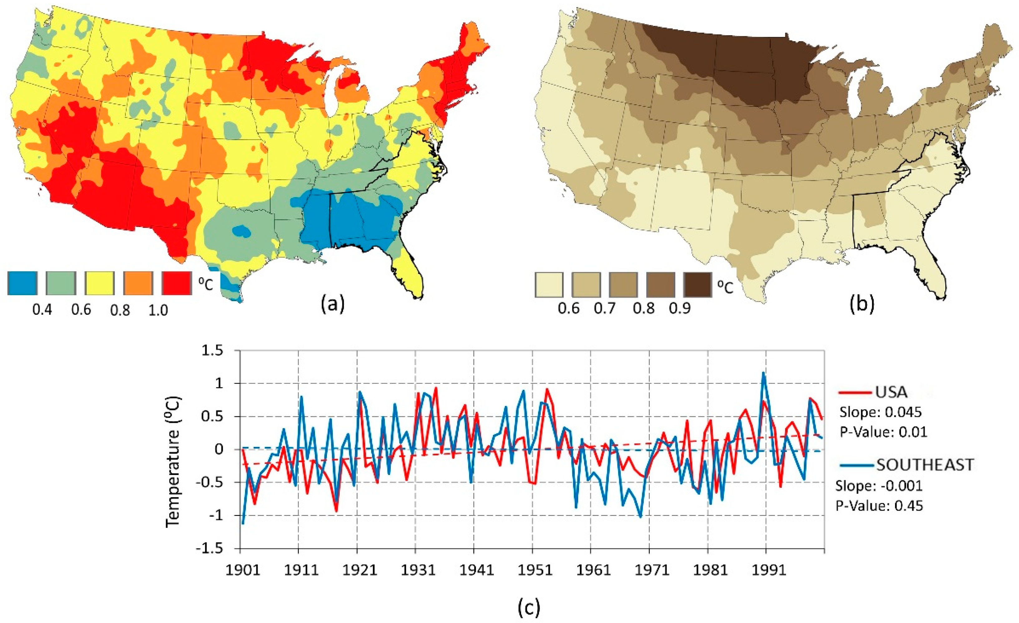
Figure 2 shows the changes and variability of annual air temperature in the conterminous US during the 20th century. The spatial distribution pattern shown in Figure 2a indicates that increases in air temperature in the Southeast have been small (less than 0.4 °C), in contrast with the Southwest, Northeast, and upper Great Plains where the warming has been much more pronounced (more than 1 °C). The Southeast’s cooler trend relative to the rest of the conterminous US has been attested in several studies [42,43,67]. The region has also experienced less temperature variability than the northern and central US (Figure 2b). For both the US and the Southeast, temporal fluctuations occurred at interannual and decadal time scales during the 20th century (Figure 2c). Negative temperature anomalies dominated the early century, but they were less marked in the Southeast. Then, a warmer episode occurred during the 1930s and lasted until the early 1950s. The shift toward a cooler Southeast occurred in the late 1950s and remained almost constant during the rest of the century. Overall, while the conterminous US exhibited a statistically significant temperature increase (at the 5% level), the Southeast showed a weak and statistically insignificant decrease (Figure 2c).
Figure 3 provides a closer look at temperature trends in the Southeast during the study period. Although positive trends prevail for both maximum and minimum temperatures (Tx and Tn, respectively), increases in Tn are more widespread and larger (Figure 3a,b). Tn trends that are significant at the 5% level cover 65.8% of the study area, while significant Tx trends cover only 21.5%. Coastal areas along the Atlantic Ocean and, to a lesser extent, northern Alabama and Georgia record the largest Tn increases (larger than 0.6 °C/decade). For both Tx and Tn, statistically significant negative trends are sparsely distributed and cover small areas (3.6% and 1.3%, respectively).
To summarize, recent warming in the Southeast has been dominated by statistically significant increases in Tn. However, longer-term records from the early 20th century to the present day show that this region has been cooler than the rest of the conterminous US. Will this exception in the Southeast be valid for extreme temperature trends?
3.2. Temperature Extremes
Trend analysis results for temperature extremes are summarized in Table 2 and Figure 4. Overall, the results indicate significant positive trends for indices pointing to warmer conditions (e.g., tropical nights, warm nights). Conversely, decreases in cooler conditions are generally indicated by significant negative trends (e.g., frost days, cool nights, and cold spell duration index).
The trends shown in Table 2 are consistent with the results displayed in Figure 4. These significant changes, whether positive or negative, generally occur over large portions of the Southeast.
Next, we analyze the spatial and temporal patterns of extreme climate indices. Subsequent figures display anomaly time series (shown as plots) and trends (shown as maps) for each index.
3.2.1. Percentile-Based Indices
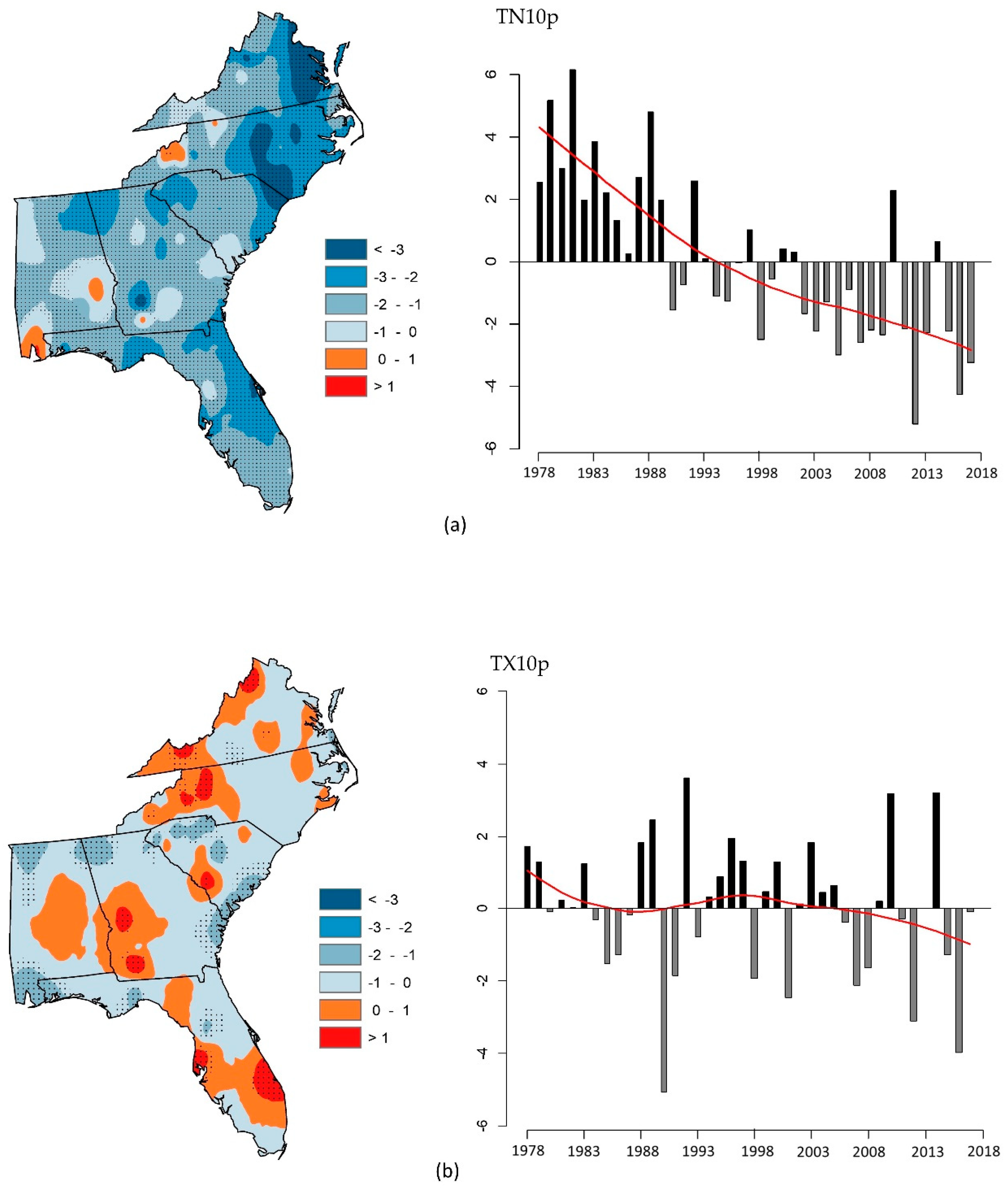
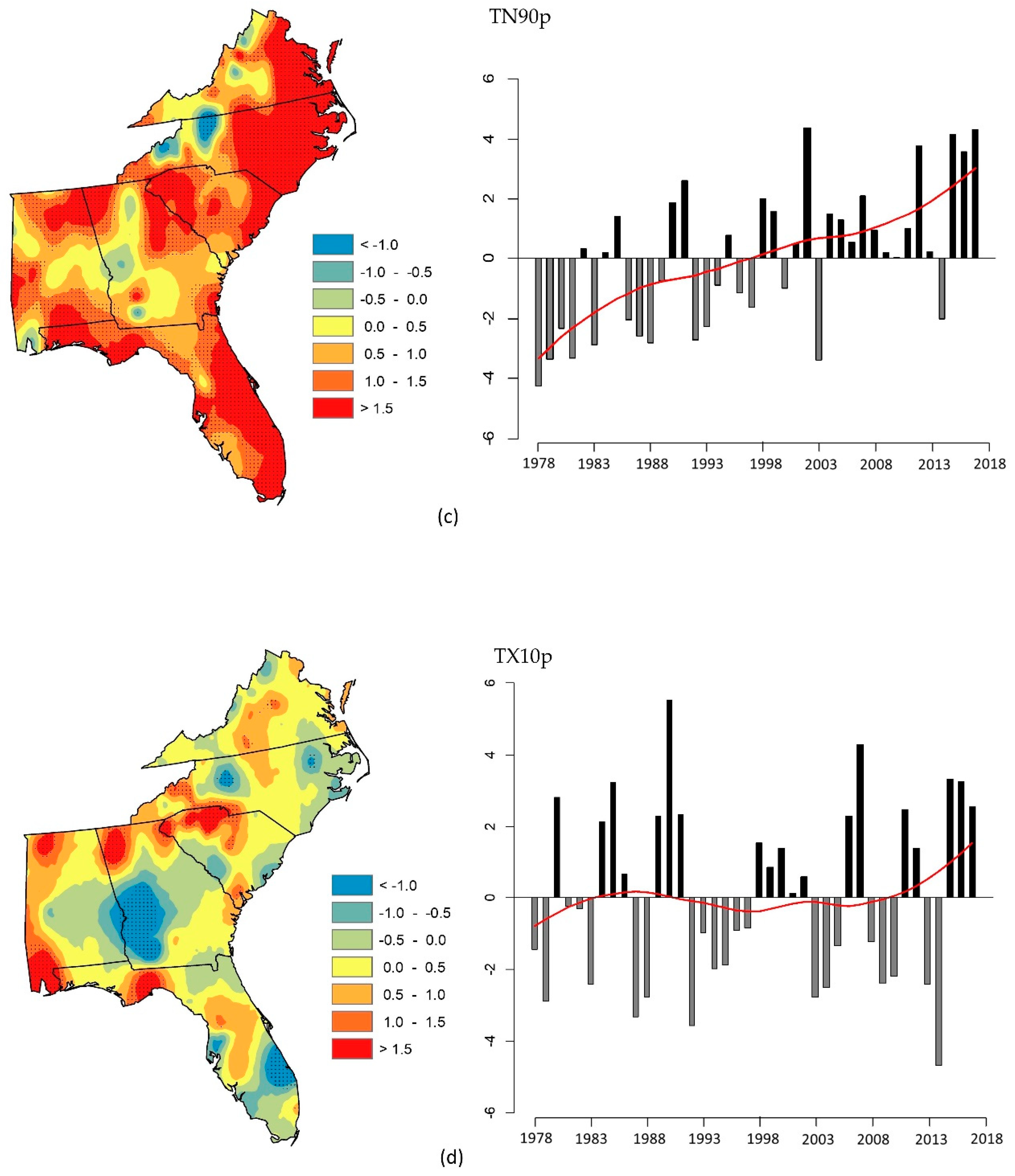
The results indicate that, in general, increasing trends in warm extremes contrast with decreases in cold extremes, and significant increases in temperature extremes associated with minimum temperatures are much more spatially widespread. Decreases in cool nights and, to a lesser extent, cool days (TN10p and TX10p, respectively) have dominated large parts of southeastern US (Figure 5a,b). Significant decreases in cool nights (at the 5% level) occurred over almost 87% of the Southeast (Figure 4). Conversely, warm nights (TN90p) exhibit statistically significant warming trends over 63% of the study area (Figure 4 and Figure 5c). Warm days (TX90p) show a more modest increase which is not statistically significant over time (Figure 5d). Significant positive TX90p trends are found in very limited regions (8.6% of the study area), especially over northern regions of North Carolina and Georgia, and western Alabama. Overall, percentile-based indices show a tendency toward warmer temperature extremes which prevail over most of the Southeast and are strongly indicated by statistically significant and widespread decreases in TN10p and increases in TN90p.
3.2.2. Absolute Indices
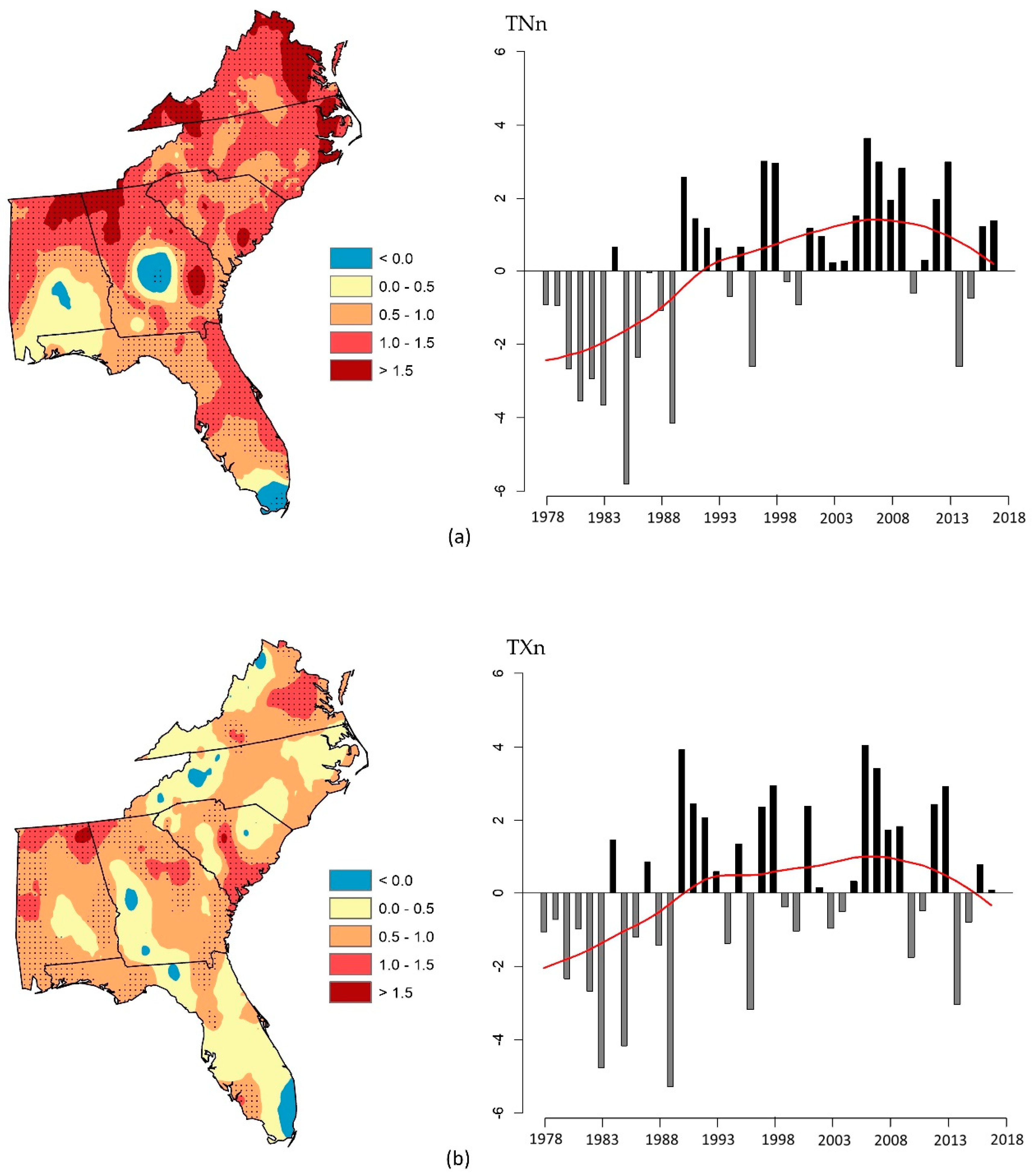
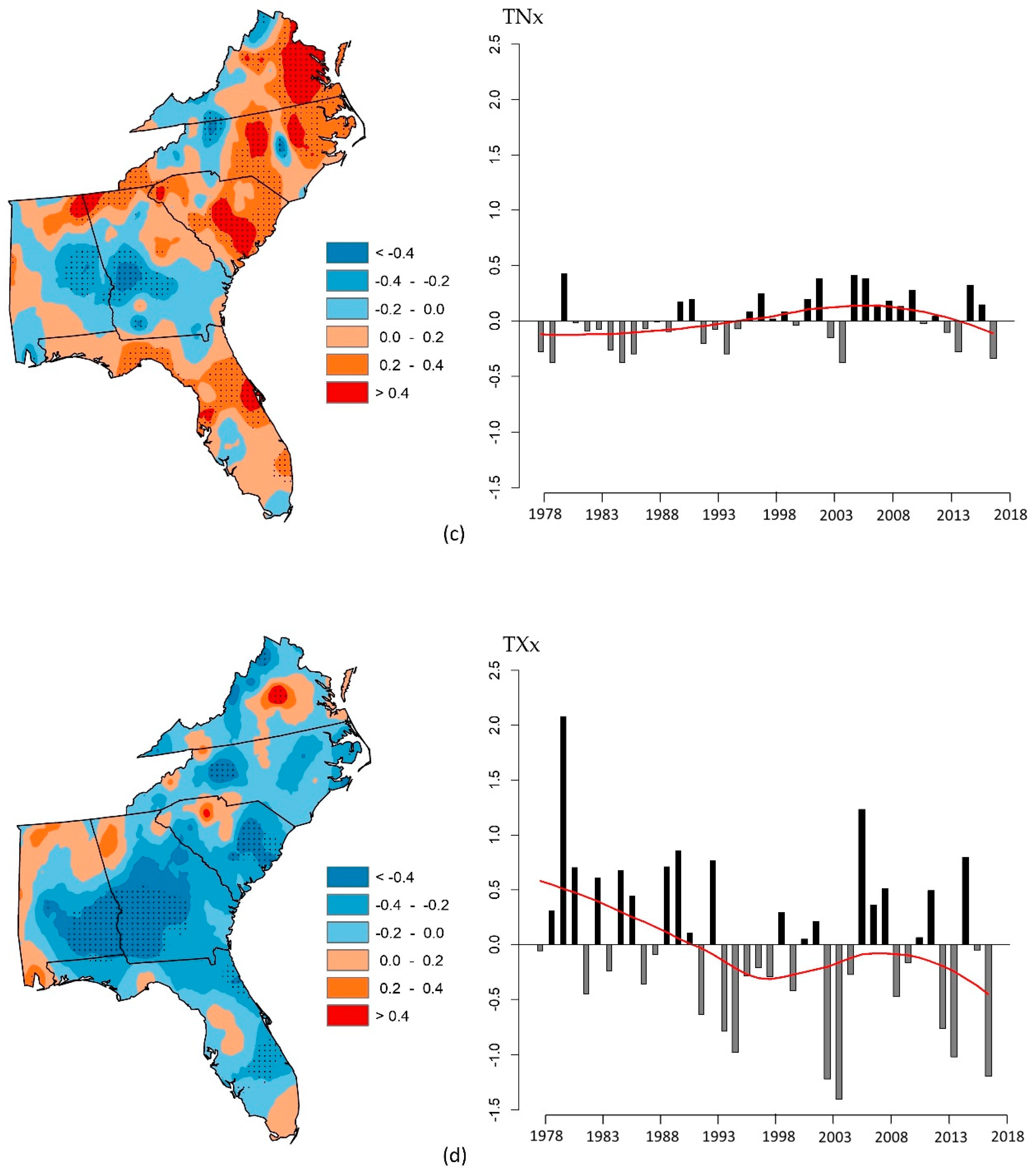
Absolute indices showing the coldest events (coldest night and day) contrast with the ones showing the warmest events (warmest night and day). The coldest night (TNn) exhibits the largest increase (a statistically significant trend of 1 °C/decade, as shown in Table 2), with 77.2% of the study area showing a significant increase (Figure 4 and Figure 6). The spatial distribution of trends points to a widespread increase for the coldest nights and days (Figure 6a,b), with the coldest nights showing the largest trend magnitude along coastal Virginia and North Carolina, western Virginia, northern Alabama, and northern Georgia. In contrast, trends for the hottest day (TXx) significantly decreased (−0.2 °C/decade), especially in central Alabama and Georgia where most of the statistically significant decrease occurred (Figure 6d). Overall, trend increases are more pronounced for the coldest night and, to a lesser extent, the coldest day, although the recent decade is dominated by a gradual decrease, as indicated by the time series in Figure 6a,b. These results are consistent with the ones found on a global scale and in many regions of the world [26,27,28,29,31].
3.3. Threshold Indices
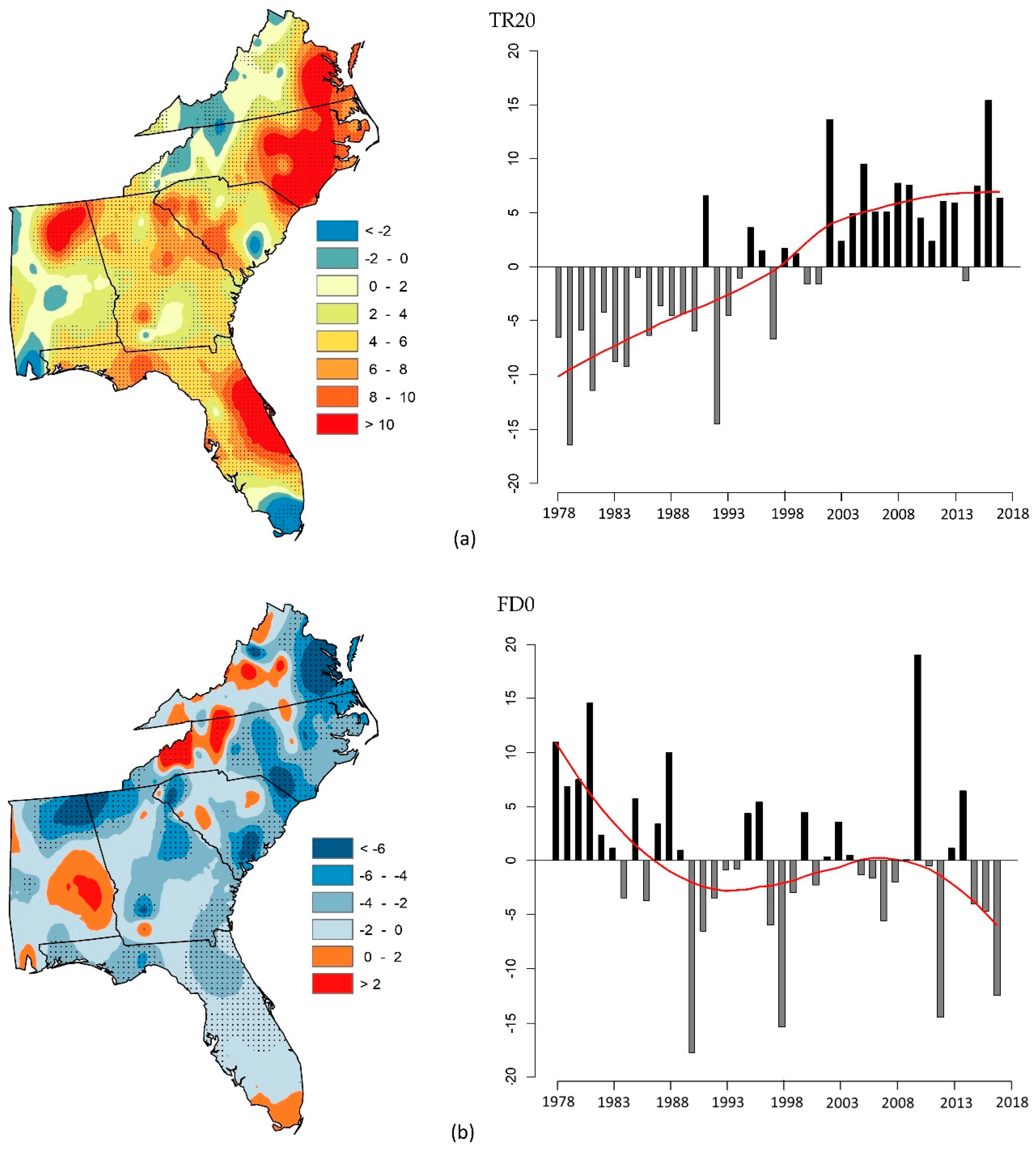
Trends for all threshold indices reflect a warming climate, as attested by the increase in warm events (tropical nights and summer days) and the decrease in cold ones (frost days and ice days) (Table 2). However, only tropical nights (TR20) trends are statistically significant (4.8 days/decade), with large portions of the Southeast showing significant increases which occur mostly along the coast (eastern Virginia and North Carolina, east-central Florida) and, to a lesser extent, northern Alabama (Figure 7a). A decrease in TR20 occurred during the period from 1978 to 2001, followed by a dramatic shift to a predominant increase since 2002. Conversely, frost days (FD0), which are related to cooling, showed negative trends that are not significant (−1.9 and −0.2 days/decade, respectively, as shown in Table 2). The spatial distribution of FD0 trends indicate a widespread predominance of decreasing trends over the Southeast, especially in northern Alabama and eastern Virginia (Figure 7b). Once again, extreme events associated with minimum temperatures exhibit stronger warming, as shown by the widespread increase in TR20 occurring over most of the Southeast (statistically significant positive trends over 67.5% of the study area).
3.4. Duration Indices
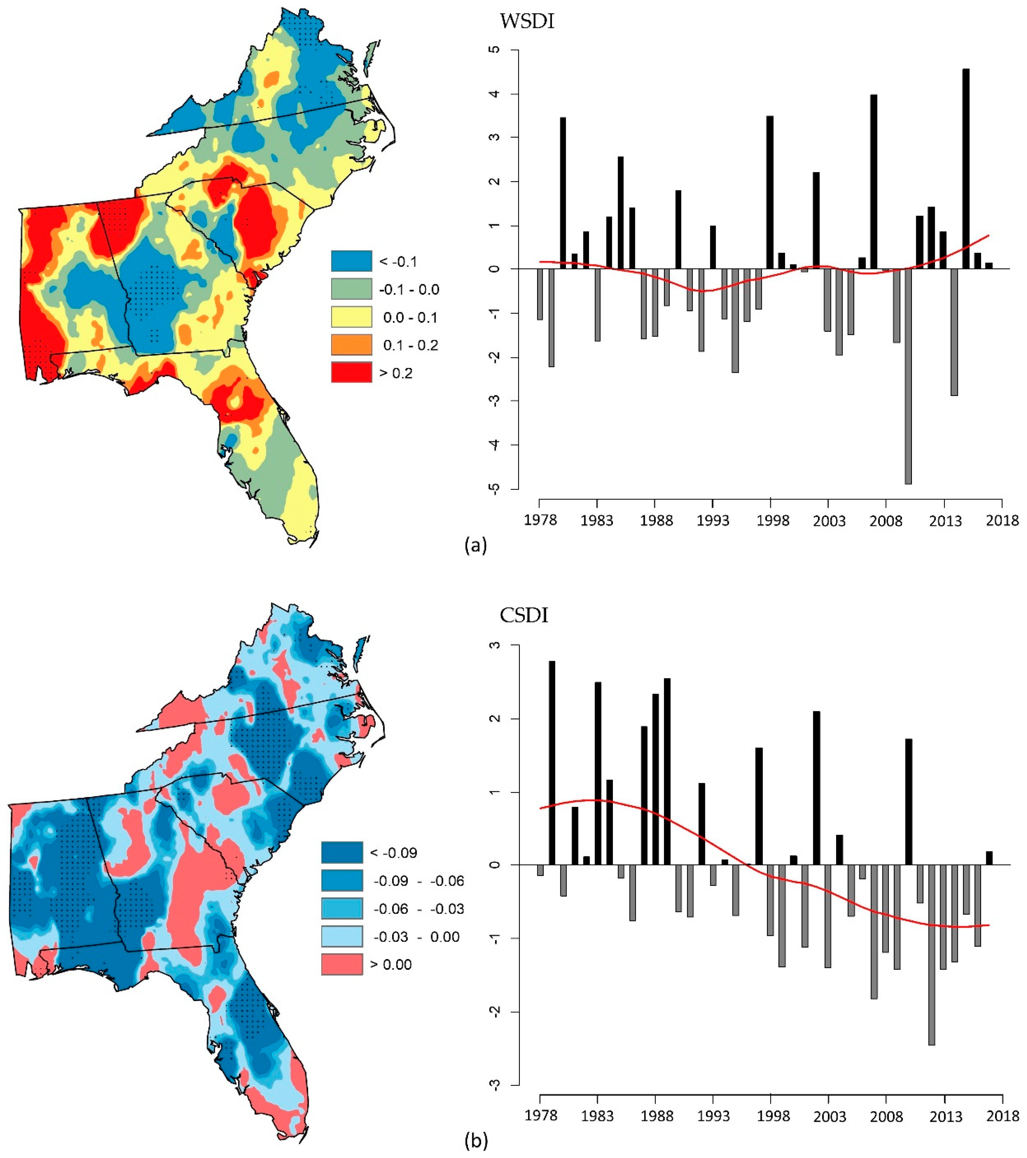
Warm spells (WSDI) show a non-significant and small increase by 0.1 days/decade (Table 2). This increase occurred mostly over western Alabama, northern Georgia, central South Carolina, and north-central Georgia (Figure 8a). A statistically significant decrease in WSDI is limited to small portions (4.6% of the Southeast) in central Georgia and the northern tip of Virginia. Overall, the spatial distribution of WSDI trends denotes mixed patterns over the Southeast, unlike the central and western parts of North America which show a more widespread and statistically significant increase in the frequency of warm spells [44]. Similarly, the associated time series depicts marked interannual variations over the study period resulting in a relatively stable trend (Figure 8a). Cold spells (CSDI) have significantly decreased at a rate of −0.6 days/decade (Table 2). Most of the decrease occurred since the late 1990s (Figure 8b). A significant trend toward less cold spells covers 18% of the Southeast, including large parts of Alabama, and is also apparent in west-central Georgia, central North Carolina, and east-central Florida. Increases in cold spells are not statistically significant and occur in scattered patches that are not spatially coherent (Figure 8b).
4. Discussion
How do findings from this study compare with other global and mostly regional studies which covered the US? Trend analysis results from this study are compared with two global studies [29,31] and one regional study by Brown et al. [67], as shown in Table 3.
Alexander et al. [29] and Donat et al. [31] computed climate extreme indices from in-situ observation data at global scale and then interpolated the indices to gridded surfaces. Trend values of indices were not presented as a table, but a selected set was shown through maps from which trends over southeastern US can be inferred.
Alexander et al. [29] presented trend maps of eight indices for 1951–2003. Their findings concur with ours for four indices: a decrease in cool nights (TN10P) and frost days (FD), and an increase in warm nights (TN90P) (Table 3). However, while this study found that trends of the aforementioned indices are significant (except for FD), those from Alexander et al. [44] over the Southeast are not. In contrast with our study, Alexander et al. [29] found a non-significant decrease in warm days (TX90P) and upward trends for cool days (TX10P) and cold spells (CSDI) over the Southeast. A comparison of warm spells trends (WSDI) is not straightforward because, while this study found a non-significant increase in WSDI, the patterns of trend distribution found by Alexander et al. [29] are not spatially coherent over the Southeast. Overall, the comparison between the two studies indicates that ours found a more pronounced warming of the Southeast.
Comparing this study’s trend results over the Southeast with those from Donat et al. [31] over the same area indicate an agreement in trend sign and magnitude for six indices; both studies found a trend decrease in the hottest day (TXx), cool nights (TN10P), and cold spells (CSDI), and an increase in the warmest night (TNx), the coldest night (TNn), and warm nights (TN90P) (Table 3). Trends in TN10P and TN90P are statistically significant in both studies. Discrepancies between the two studies consist of trends of opposite signs for four indices. Donat et al. [31] found non-significant trend decreases in the coldest day (TXn), warm days (TX90P), and warm spells (WSDI), and a non-significant increase in cool days (TX10P). In contrast, this study found trends of opposite signs for these indices, including a statistically significant increase in TXn trend over the Southeast.
Overall, the trend comparison with both global studies [29,31] indicates that this study found a more pronounced warming of the Southeast. Both global studies constitute an excellent reference for those looking into trends in climate extremes during the 20th and early 21st centuries. However, extreme indices in these studies were gridded at a coarse resolution, which is common with global datasets.
Regional studies of temperature extremes in the United States include a relatively early study by Karl et al. [41] who developed a Climate Extremes Index (CEI) which led to the conclusion that the US climate was becoming more extreme. The CEI was revised by Gleason et al. [2] who included auxiliary station data, extended the index further back in time, and improved its spatial coverage. More recent regional studies for the United States are generally based on gridded data. For example, Wuebbles et al. [68] used CMIP5-simulated historical and projected future trends in extreme temperatures over the contiguous US and found that extreme temperature indices point to increases in the frequency of high extremes and decreases in low extremes. To investigate teleconnections between winter climate extremes and large-scale modes of climate variability over the northeastern US and southeastern Canada, Ning and Bradley [69] computed temperature extreme indices using high resolution gridded data from Maurer et al. [70]. Ning et al. [71] examined future changes in climate extremes over northeastern US using downscaled extreme indices calculated by various general circulation models from phase 5 of the Coupled Model Intercomparison Project (CMIP5). The results showed increasing (decreasing) warm (cold) extremes.
Studies using observations to compute climate extreme indices at station level over the US are still scarce. One such study by Griffiths and Bradley [72] used USHCN station observations to examine variations of temperature and precipitation extremes over northeastern US (1926–2000). However, only five temperature indices were analyzed. The authors split the study period into several intervals and found varying trend changes depending on the periods. In a subsequent study, Brown et al. [67] computed 16 temperature extreme indices from daily data obtained from 40 USHCN stations to analyze changes in extreme climate indices for the northeastern US. The authors computed trends for the extreme indices over various periods, including from 1951–2005. Therefore, not only does their study period partly overlap with ours, but it also uses data from the same source (USHCN) and covers a region that is almost adjacent to the Southeast. Table 3 indicates that climate extreme trends from Brown et al. [67] compare very well with the ones from this study. Out of the 16 indices analyzed, there is an agreement on trend sign for 12 indices. Very few trend differences exist between the two studies: (i) this study found a statistically significant negative trend for the hottest day index (TXx), and a statistically significant upward trend for the coldest day index (TXn), whereas Brown et al. [67] found no trend for both indices; (ii) trends of warm spells (WSDI) are of opposite signs in the two studies, as there was a non-significant increase over the Southeast (this study) and a decreasing trend in the Northeast (Brown et al. [67]). Overall, the trend sign comparison suggests that the Southeast appeared to exhibit more warming than the Northeast; trends of indices point to a larger increase in warm extremes and a steeper decline of cool extremes. Regarding the percentage of land with positive and negative trends that are significant at the 5% level, values are in general proportionally consistent: in both studies, (i) warm nights, tropical nights, and the coldest night are among indices which cover the largest portion of land with significantly positive trends; and (ii) cool nights, frost days, and cold spells cover the largest land areas with significantly negative trends.
To summarize, except for very few differences, this study’s findings regarding trend sign and magnitude are generally consistent with previous global and regional studies.
5. Conclusions
This study has presented an assessment of climate variability and climate extremes over 40 years (1978–2017) for southeastern USA, a region that currently experiences modest warming trends, although the long-term surface temperatures have shown a predominantly cooling trend. In agreement with previous studies, the results indicate that, in general, (i) increasing trends in warm extremes contrast with decreases in cold extremes, and (ii) significant increases in temperature extremes associated with minimum temperatures are of larger magnitude and are more spatially widespread than the ones associated with maximum temperatures.
To summarize, the tendency toward warming is apparent as attested by increasing trends in the annual occurrence of the warmest night, warm days, warm nights, tropical nights, and warm spells. In particular, statistically significant increases in tropical nights and warm nights occurred over larger portions of the Southeast. Conversely, most cold extremes showed negative trends, including cool nights, cool days, frost days, and cold spells. The largest negative trend magnitude is attributed to frost days, but the change is not significant. Cool nights exhibit a significant decrease and the largest percentage of negative trends over the study area (87.2%).
However, the tendency toward warmer extremes is not uniform, in particular regarding absolute indices: (i) there was a significant increase in the coldest nights over most of the Southeast (77.4% of the study area); (ii) the coldest day also showed significant negative trends; and (iii) there was a significant decrease in the hottest day.
Given differences in the study area, period, and methods used to compute trends, the comparison with other studies is not straightforward. However, increases in warm temperature extremes and decreases in cold ones found in this study are consistent with changes in extremes found across other US regions and on a global scale. Therefore, this study shows that being part of the ’warming hole’ does not preclude southeastern US from an intensification of most temperature extremes. Further, trend patterns of temperature extremes indicate that the Southeast is presently warming and that, in the future, this region may not constitute an exception anymore. Increases in tropical nights and warm nights, and decreases in cool nights and frost days exhibit coherent spatial patterns, display outstanding characteristics of the region’s temperature extremes, and are consistent with results from a large body of studies.
Studies conducted on a global scale provide an overall view and are good at capturing the big picture of climatic phenomena, but do not allow detailed analysis on a finer scale. To date, although there is already a large number of studies about trends in climate extremes, this is the only subregional study which conducted such investigation over southeastern US using quality-controlled observations. Moreover, while most studies focus on changes in extreme climate events over time, in this study we analyze climate extremes over specific areas where temperature trends have exhibited anomalous behavior. This is a first steps toward understanding how temperature extremes relate to the characteristics of their corresponding climate zones.
Author Contributions
Conceptualization, S.F. and K.M.C.; methodology, S.F., K.M.C., J.E.Q. and G.E.A.; software, S.F. and K.M.C.; validation, S.F., K.M.C., J.E.Q., G.E.A. and R.A.; formal analysis, S.F.; investigation, S.F.; resources, S.F., K.M.C., J.E.Q., G.E.A. and R.A.; data curation, S.F.; writing—original draft preparation, S.F.; writing—review and editing, S.F., J.E.Q., K.M.C., G.E.A. and R.A.; visualization, S.F.; supervision, S.F.; project administration, S.F.; funding acquisition, S.F., J.E.Q., G.E.A. and R.A. All authors have read and agreed to the published version of the manuscript.
Funding
This study was supported by USDA-NIFA, Grants #11343629 and #1001194. We also gratefully acknowledge the support from Tuskegee University’s George Washington Carver Agricultural Experiment Station.
Data Availability Statement
The gridded indices will be available upon request addressed to Souleymane Fall.
Conflicts of Interest
The authors declare no conflict of interest. The funders had no role in the design of the study; in the collection, analyses, or interpretation of data; in the writing of the manuscript, or in the decision to publish the results.
References
- Stocker, T.F.; Qin, D.; Plattner, G.-K.; Alexander, L.V.; Allen, S.K.; Bindoff, N.L.; Bréon, F.-M.; Church, J.A.; Cubasch, U.; Emori, S.; et al. Technical summary. In Climate Change 2013: The Physical Science Basis. Contribution of Working Group I to the Fifth Assessment Report of the Intergovernmental Panel on Climate Change; Stocker, T.F., Qin, D., Plattner, G.K., Tignor, M., Allen, S.K., Boschung, J., Nauels, A., Xia, Y., Bex, V., Midgley, P.M., Eds.; Cambridge University Press: Cambridge, UK, 2013; pp. 33–115. [Google Scholar] [CrossRef]
- Gleason, K.L.; Lawrimore, J.H.; Levinson, D.H.; Karl, T.R.; Karoly, D.J. A Revised, U.S. Climate Extremes Index. J. Clim. 2008, 21, 2124–2137. [Google Scholar] [CrossRef] [Green Version]
- Herring, S.C.; Hoell, A.; Hoerling, M.P.; Kossin, J.P.; Schreck III, C.J.; Stott, P.A. Explaining Extreme Events of 2015 from a Climate Perspective. Bull. Amer. Meteor. Soc. 2016, 97, S1–S145. [Google Scholar] [CrossRef] [Green Version]
- Hoerling, M.; Eischeid, J.; Perlwitz, J.; Quan, X.; Wolter, K. Characterizing recent trends in U.S. heavy precipitation. J. Clim. 2016, 29, 2313–2332. [Google Scholar] [CrossRef]
- World Meteorological Organization. Atlas of Mortality and Economic Losses from Weather and Climate Extremes. 1970–2012; WMO: Geneva, Switzerland, 2014; p. 1123. [Google Scholar]
- Sheridan, S.C.; Allen, M.J. Changes in the Frequency and Intensity of Extreme Temperature Events and Human Health Concerns. Curr. Clim. Chang. Rep. 2005, 1, 155–162. [Google Scholar] [CrossRef]
- Wallemacq, P.; Below, R.; Mcclean, D. UNISDR and CRED report: Economic Losses, Poverty & Disasters 1998–2017; Centre for Research on the Epidemiology of Disasters, CRED: Brussels, Belgium, 2018; Available online: https://www.preventionweb.net/files/61119_credeconomiclosses.pdf (accessed on 21 November 2019).
- Vogel, E.; Donat, M.G.; Alexander, L.V.; Meinshausen, M.; Ray, D.K.; Karoly, D.; Meinshausen, N.; Frieler, K. The effects of climate extremes on global agricultural yields. Environ. Res. Lett. 2019, 14, 054010. [Google Scholar] [CrossRef]
- Rorie, A.C.; Poole, J. The Role of Extreme Weather and Climate-Related Events on Asthma Outcomes. Immunol Allergy Clin. North Am. 2021, 41, 73–84. [Google Scholar] [CrossRef]
- Weilnhammer, V.; Schmid, J.; Mittermeier, I.; Schreiber, F.; Jiang, L.; Pastuhovic, V.; Herr, C.; Heinze, S. Extreme weather events in Europe and their health consequences—A systematic review. Int. J. Hyg. Environ. Health 2021, 233, 113688. [Google Scholar] [CrossRef]
- IPCC. Managing the Risks of Extreme Events and Disasters to Advance Climate Change Adaptation; A Special Report of Working Groups I and II of the Intergovernmental Panel on Climate Change; Field, C.B., Barros, V., Stocker, T.F., Qin, D., Dokken, D.J., Ebi, K.L., Mastrandrea, M.D., Mach, K.J., Plattner, G.-K., Allen, S.K., et al., Eds.; Cambridge University Press: Cambridge, UK; New York, NY, USA, 2012; 582p. [Google Scholar]
- Frank, D.; Reichstein, M.; Bahn, M.; Thonicke, K.; Frank, D.; Mahecha, M.D.; Smith, P.; van der Velde, M.; Vicca, S.; Babst, F.; et al. Effects of climate extremes on the terrestrial carbon cycle: Concepts, processes and potential future impacts. Glob. Chang. Biol. 2015, 21, 2861–2880. [Google Scholar] [CrossRef] [Green Version]
- Aragão, L.E.O.C.; Marengo, J.A.; Cox, P.M.; Betts, R.A.; Costa, D.; Kaye, N.; Alves, L.; Smith, L.T.; Cavalcanti, I.F.A.; Sampaio, G.; et al. Assessing the Influence of Climate Extremes on Ecosystems and Human Health in Southwestern Amazon Supported by the PULSE Brazil Platform. Am. J. Clim. Chang. 2016, 5, 399–416. [Google Scholar] [CrossRef] [Green Version]
- Mitchell, D.M.; Heaviside, C.; Vardoulakis, S.; Huntingford, C.; Masato, G.; Guillod, B.P.; Frumhoff, P.C.; Bowery, A.; Allen, M.R. Attributing human mortality during extreme heat waves to anthropogenic climate change. Environ. Res. Lett. 2016, 11, 074006. [Google Scholar] [CrossRef]
- Karl, T.R.; Nicholls, N.; Ghazi, A. CLIVAR/GCOS/WMO workshop on indices and indicators for climate extremes. Clim. Chang. 1999, 42, 3–7. [Google Scholar] [CrossRef]
- Nicholls, N. Long-term climate monitoring and extreme events. Clim. Chang. 1995, 31, 231–245. [Google Scholar] [CrossRef]
- Jones, P.D.; Horton, E.B.; Folland, C.K.; Hulme, M.; Parker, D.E.; Basnett, T.A. The use of indices to identify changes in climatic extremes. Clim. Chang. 1999, 42, 131–149. [Google Scholar] [CrossRef]
- Groisman, P.; Karl, T.; Easterling, D.; Knight, R.; Jamason, P.; Hennessy, K.; Suppiah, R.; Page, C.; Wibig, J.; Fortuniak, K.; et al. Changes in the probability of extreme precipitation: Important indicators of climate change. Clim. Chang. 1999, 42, 243–283. [Google Scholar] [CrossRef]
- Frich, P.; Alexander, L.V.; Della-Marta, P.M.; Gleason, B.; Haylock, M.; Tank, A.M.G.K.; Peterson, T. Observed coherent changes in climatic extremes during the second half of the twentieth century. Clim. Res. 2002, 19, 193–212. [Google Scholar] [CrossRef] [Green Version]
- Peterson, T.C.; Manton, M.J. Monitoring changes in climate extremes: A tale of international collaboration. Bull. Am. Meteorol. Soc. 2008, 89, 1266–1271. [Google Scholar] [CrossRef]
- Klein Tank, A.M.G.; Zwiers, F.W.; Zhang, X. Guidelines on Analysis of Extremes in a Changing Climate in Support of Informed Decisions for Adaptation; Climate Data and Monitoring WCDMP-No. 72, WMO-TD No. 1500; World Meteorological Organization: Geneva, Switzerland, 2009. [Google Scholar]
- Peterson, T.C. Climate change indices. World Meteorol. Organ. Bull. 2005, 54, 83–86. [Google Scholar]
- Peterson, T.C.; Taylor, M.A.; Demeritte, R.; Duncombe, D.L.; Burton, S.; Thompson, F.; Porter, A.; Mercedes, M.; Villegas, E.; Fils, R.S.; et al. Recent changes in climate extremes in the Caribbean region. J. Geophys. Res. 2002, 107, 4601. [Google Scholar] [CrossRef]
- Nicholls, N.; Baek, H.-J.; Gosai, A.; Chambers, L.E.; Choi, Y.; Collins, D.; Della-Marta, P.M.; Griffiths, G.M.; Haylock, M.R.; Iga, N.; et al. The El Niño-Southern Oscillation and daily temperature extremes in east Asia and the west Pacific. Geophys. Res. Lett. 2005, 32, L16714. [Google Scholar] [CrossRef] [Green Version]
- Zhang, X.; Aguilar, E.; Sensoy, S.; Tonyan, H.; Tagiyeva, U.; Ahmed, N.; Kutaladze, N.; Rahimzadeh, F.; Taghipour, A.; Hantosh, T.H.; et al. Trends in Middle East climate extreme indices from 1950 to 2003. J. Geophys. Res. 2005, 110, D22104. [Google Scholar] [CrossRef]
- Aguilar, E.; Peterson, T.C.; Obando, P.R.; Frutos, R.; Retana, J.A.; Solera, M.; Soley, J.; García, I.G.; Araujo, R.M.; Santos, A.R.; et al. Changes in Precipitation and Temperature Extremes in Central America and Northern South America, 1961–2003. J. Geophys. Res. 2005, 110, D23107. [Google Scholar] [CrossRef]
- Klein Tank, A.M.G.; Peterson, T.C.; Quadir, D.A.; Dorji, S.; Zou, X.; Tang, H.; Santhosh, K.; Joshi, U.R.; Jaswal, A.K.; Kolli, R.K.; et al. Changes in daily temperature and precipitation extremes in central and south Asia. J. Geophys. Res. Atmos. 2006, 111. [Google Scholar] [CrossRef]
- Caesar, J.; Alexander, L.V.; Trewin, B.; Tse-ring, K.; Sorany, L.; Vuniyayawa, V.; Keosavang, N.; Shimana, A.; Htay, M.M.; Karmacharya, J.; et al. Changes in temperature and precipitation extremes over the Indo-Pacific region from 1971–2005. Int. J. Climatol. 2011, 31, 791–801. [Google Scholar] [CrossRef]
- Alexander, L.V.; Zhang, X.; Peterson, T.C.; Caesar, J.; Gleason, B.; Klein Tank, A.; Haylock, M.; Collins, D.; Trewin, B.; Rahimzadeh, F.; et al. Global Observed Changes in Daily Climate Extremes of Temperature and Precipitation. J. Geophys. Res. 2006, 111, D05109. [Google Scholar] [CrossRef] [Green Version]
- Alexander, L.V.; Arblaster, J.M. Assessing trends in observed and modelled climate extremes over Australia in relation to future projections. Int. J. Climatol. 2009, 29, 417–435. [Google Scholar] [CrossRef]
- Donat, M.G.; Alexander, L.V.; Yang, H.; Durre, I.; Vose, R.; Dunn, R.J.H.; Willett, K.M.; Aguilar, E.; Brunet, M.; Caesar, J.; et al. Updated analyses of temperature and precipitation extreme indices since the beginning of the twentieth century: The HadEX2 dataset. J. Geophys. Res. Atmos. 2013, 118, 2098–2118. [Google Scholar] [CrossRef]
- Herold, N.; Alexander, L.V.; Green, D.; Donat, M.G. Greater increases in temperature extremes in low versus high income countries. Environ. Res. Lett. 2017, 12, 034007. [Google Scholar] [CrossRef] [Green Version]
- Costa, R.L.; de Mello Baptista, G.M.; Gomes, H.B.; dos Santos Silva, F.D.; da Rocha Júnior, R.L.; de Araújo Salvador, M.; Herdies, D.L. Analysis of climate extremes indices over northeast Brazil from 1961 to 2014. Weather Clim. Extrem. 2020, 28, 100254. [Google Scholar] [CrossRef]
- Peña-Angulo, D.; Reig-Gracia, F.; Domínguez-Castro, F.; Revuelto, J.; Aguilar, E.; van der Schrier, G.; Vicente-Serrano, S.M. ECTACI: European climatology and trend atlas of climate indices (1979–2017). J. Geophys. Res. Atmos. 2020, 125, e2020JD032798. [Google Scholar] [CrossRef]
- Easterling, D.R. Recent changes in frost days and the frost-free season in the United States. Bull. Am. Meteorol. Soc. 2002, 83, 1327–1332. [Google Scholar] [CrossRef]
- Pan, Z.; Arritt, R.W.; Takle, E.S.; Gutowski, W.J., Jr.; Anderson, C.J.; Segal, M. Altered hydrologic feedback in a warming climate introduces a “warming hole”. Geophys. Res. Lett. 2004, 31, L17109. [Google Scholar] [CrossRef] [Green Version]
- Portmann, R.W.; Solomon, S.; Hegerl, G.C. Spatial and seasonal patterns in climate change, temperatures, and precipitation across the United States. Proc. Natl. Acad. Sci. USA 2009, 106, 7324–7329. [Google Scholar] [CrossRef] [Green Version]
- Meehl, G.A.; Arblaster, J.; Branstator, G.W. Mechanisms contributing to the warming hole and the consequent U.S. east-west differential of heat extremes. J. Clim. 2012, 25, 6394–6408. [Google Scholar] [CrossRef]
- Mascioli, N.R.; Previdi, M.; Arlene, M.; Fiore, A.M.; Ting, M. Timing and seasonality of the United States ‘warming hole’. Environ. Res. Lett. 2017, 12, 034008. [Google Scholar] [CrossRef] [Green Version]
- Banerjee, A.; Polvani, L.M.; Fyfe, J.C. The United States “warming hole”: Quantifying the forced aerosol response given large internal variability. Geophys. Res. Lett. 2017, 44, 1928–1937. [Google Scholar] [CrossRef]
- Karl, T.R.; Knight, R.W.; Easterling, D.R.; Quayle, R.G. Indices of climate change for the United States. Bull. Am. Meteorol. Soc. 1996, 77, 279–292. [Google Scholar] [CrossRef] [Green Version]
- Trenberth, K.E.; Jones, P.D.; Ambenje, P.; Bojariu, R.; Easterling, D.; Klein Tank, A.; Parker, D.; Rahimzadeh, F.; Renwick, J.A.; Rusticucci, M.; et al. Observations: Surface and Atmospheric Climate Change. In Climate Change 2007: The Physical Science Basis. Contribution of Working Group I to the Fourth Assessment Report of the Intergovernmental Panel on Climate Change; Solomon, S., Qin, D., Manning, M., Chen, Z., Marquis, M., Averyt, K.B., Tignor, M., Miller, H.L., Eds.; Cambridge University Press: Cambridge, UK; New York, NY, USA, 2007. [Google Scholar]
- Rogers, J.C. The 20th century cooling trend over the southeastern United States. Clim. Dyn. 2012, 40, 341–352. [Google Scholar] [CrossRef]
- Misra, V.; Michael, J.-P.; Boyles, R.; Chassignet, E.P.; Griffin, M.; O’Brien, J.J. Reconciling the spatial distribution of the surface temperature trends in the southeastern United States. J. Clim. 2012, 25, 3610–3618. [Google Scholar] [CrossRef] [Green Version]
- Seneviratne, S.I.; Nicholls, N.; Easterling, D.; Goodess, C.M.; Kanae, S.; Kossin, J.; Luo, Y.; Marengo, J.; McInnes, K.; Rahimi, M.; et al. Changes in climate extremes and their impacts on the natural physical environment. In Managing the Risks of Extreme Events and Disasters to Advance Climate Change Adaptation; A Special Report of Working Groups I and II of the Intergovernmental Panel on Climate Change (IPCC); Field, C.B., Barros, V., Stocker, T.F., Qin, D., Dokken, D.J., Ebi, K.L., Mastrandrea, M.D., Mach, K.J., Plattner, G.-K., Allen, S.K., et al., Eds.; Cambridge University Press: Cambridge, UK; New York, NY, USA, 2012; pp. 109–230. [Google Scholar]
- Zwiers, F.W.; Alexander, L.V.; Hegerl, G.C.; Kossin, J.P.; Knutson, T.R.; Naveau, P.; Nicholls, N.; Schär, C.; Seneviratne, S.I.; Zhang, X.; et al. Challenges in estimating and understanding recent changes in the frequency and intensity of extreme climate and weather events. In Climate Science for Serving Society: Research, Modelling and Prediction Priorities; Asrar, G.R., Hurrell, J.W., Eds.; Springer: Dordrecht, The Netherlands; Heidelberg, Germany; New York, NY, USA; London, UK, 2013; pp. 339–389. ISBN 978-94-007-6691-4. [Google Scholar]
- Alexander, L.V. Global observed long-term changes in temperature and precipitation extremes: A review of progress and limitations in IPCC assessments and beyond. Weather Clim. Extrem. 2016, 11, 4–16. [Google Scholar] [CrossRef] [Green Version]
- Davey, C.A.; Pielke, R.A., Sr. Microclimate exposures of surface-based weather stations: Implications for the assessment of long-term temperature trends. Bull. Am. Meteorol. Soc. 2005, 86, 497–504. [Google Scholar] [CrossRef] [Green Version]
- Pielke, R.A., Sr.; Nielsen-Gammon, J.; Davey, C.; Angel, J.; Bliss, O.; Cai, M.; Doesken, N.; Fall, S.; Niyogi, D.; Gallo, K.; et al. Documentation of uncertainties and biases associated with surface temperature measurement sites for climate change assessment. Bull. Am. Meteorol. 2007, 88, 913–928. [Google Scholar] [CrossRef] [Green Version]
- Pielke, R.A., Sr.; Davey, C.; Niyogi, D.; Fall, S.; Steinweg-Woods, J.; Hubbard, K.; Lin, X.; Cai, M.; Lim, Y.K.; Li, H.; et al. Unresolved issues with the assessment of multi-decadal global land surface temperature trends. J. Geophys. Res. 2007, 112, D24S08. [Google Scholar] [CrossRef]
- Fall, S.; Watts, A.; Nielsen-Gammon, J.; Jones, E.; Niyogi, D.; Christy, J.R.; McNider, R.; Pielke, R.A., Sr. Analysis of the impacts of station exposure on the U.S. Historical Climatology Network temperatures and temperature trends. J. Geophys. Res. 2011, 116, D14120. [Google Scholar] [CrossRef] [Green Version]
- Thorne, P.W.; Parker, D.E.; Christy, J.R.; Mears, C.A. Uncertainties in climate trends: Lessons from upper-air temperature records. Bull. Am. Meteorol. Soc. 2005, 86, 1437–1442. [Google Scholar] [CrossRef]
- Menne, M.J.; Williams, C.N.; Vose, R.S. The United States Historical Climatology Network Monthly Temperature Data—Version 2. Bull. Am. Meteorol. Soc. 2009, 90, 993–1107. [Google Scholar] [CrossRef] [Green Version]
- Lawrimore, J.H.; Menne, M.J.; Gleason, B.E.; Williams, C.N.; Wuertz, D.B.; Vose, R.S.; Rennie, J. An overview of the Global Historical Climatology Network Monthly Mean Temperature Dataset, Version 3. J. Geophys. Res. Atmos. 2011, 116, D19121. [Google Scholar] [CrossRef]
- Karl, T.R.; Williams, C.N., Jr.; Quinlan, F.T. United States Historical Climatology Network (HCN) Serial Temperature and Precipitation Data; ORNL/CDIAC-30; Carbon Dioxide Information Analysis Center, Oak Ridge National Laboratory, U.S. Department of Energy: Oak Ridge, TN, USA, 1990.
- Easterling, D.R.; Karl, T.R.; Mason, E.H.; Hughes, P.Y.; Bowman, D.P. ORNL/CDIAC-87; Carbon Dioxide Information Analysis Center, Oak Ridge National Laboratory, U.S. Department of Energy: Oak Ridge, TN, USA, 1996. Available online: https://www.osti.gov/scitech/biblio/205081 (accessed on 14 November 2019).
- Menne, M.J.; Williams, C.N. Homogenization of temperature series via pairwise comparisons. J. Clim. 2009, 22, 1700–1717. [Google Scholar] [CrossRef] [Green Version]
- Zhang, X.; Yang, F. RClimDex (1.0) User Guide; Climate Research Branch Environment Canada: Downsview, ON, Canada, 2004; 22p.
- Zhang, X.; Hegerl, G.; Zwiers, F.W.; Kenyon, J. Avoiding inhomogeneity in percentile-based indices of temperature extremes. J. Clim. 2005, 18, 1641–1651. [Google Scholar] [CrossRef] [Green Version]
- Aguilar, E.; Prohom, M. RClimDex-Extra QC (EXTRAQC Quality Control Software) User Manual; Centre for Climate Change, University Rovira i Virgili: Tarragona, Spain, 2011. [Google Scholar]
- Karl, T.R.; Koscielny, A.J. Drought in the United States: 1895–1981. J. Clim. 1982, 2, 313–329. [Google Scholar] [CrossRef]
- Karl, T.R.; Koss, W.J. Regional and National Monthly, Seasonal and Annual Temperature Weighted by Area, 1895–1983; Hist. Climatol. Series 4–3; National Climatic Data Center: Ashville, NC, USA, 1984. [Google Scholar]
- Lee, S.; Wolberg, G.; Shin, S.Y. Scattered data interpolation with multilevel B-splines. IEEE Trans. Vis. Comput. Graph. 1997, 3, 228–244. [Google Scholar] [CrossRef] [Green Version]
- Cleveland, W.S. Robust locally weighted regression and smoothing scatterplots. J. Am. Stat. Assoc. 1979, 74, 829–836. [Google Scholar] [CrossRef]
- Sen, P.K. Estimates of the regression coefficient based on Kendall’s tau. J. Am. Statist. Assoc. 1968, 63, 1379–1389. [Google Scholar] [CrossRef]
- Kendall, M.G. Rank Correlation Methods; Charles Griffin: London, UK, 1948. [Google Scholar]
- Brown, P.J.; Bradley, R.S.; Keimig, F.T. Changes in extreme climate indices for the northeastern United States, 1870–2005. J. Clim. 2010, 23, 6555–6572. [Google Scholar] [CrossRef]
- Wuebbles, D.; Meehl, G.; Hayhoe, K.; Karl, T.R.; Kunkel, K.; Santer, B.; Wehner, M.; Colle, B.; Fischer, E.M.; Fu, R.; et al. CMIP5 Climate Model Analyses: Climate Extremes in the United States. Bull. Am. Meteorol. Soc. 2014, 95, 571–583. [Google Scholar] [CrossRef] [Green Version]
- Ning, L.; Bradley, R.S. Winter climate extremes over the northeastern United States and southeastern Canada and teleconnections with large-scale modes of climate variability. J. Clim. 2015, 28, 2475–2493. [Google Scholar] [CrossRef] [Green Version]
- Maurer, E.P.; Wood, A.W.; Adam, J.C.; Lettenmaier, D.P.; Nijssen, B. A long-term hydrologically based dataset of land surface fluxes and states for the conterminous United States. J. Clim. 2002, 15, 3237–3251. [Google Scholar] [CrossRef] [Green Version]
- Ning, L.; Riddle, E.E.; Bradley, R.S. Projected changes in climate extremes over the northeastern United States. J. Clim. 2015, 18, 2475–2493. [Google Scholar] [CrossRef] [Green Version]
- Griffiths, M.L.; Bradley, R.S. Variations of twentieth-century temperature and precipitation extreme indicators in the northeast United States. J. Clim. 2007, 20, 5401–5417. [Google Scholar] [CrossRef]
Figure 1.
Study area (the Southeast, as defined by NOAA) and climate stations used in the study. The inset map shows the location of the study area within the United States of America.
Figure 1.
Study area (the Southeast, as defined by NOAA) and climate stations used in the study. The inset map shows the location of the study area within the United States of America.

Figure 2.
(a) Observed changes in annual temperature over the conterminous United States; changes are the difference between the average for present-day and the average for the last century (2001–2017 minus 1901–2000); (b) annual temperature variability (1901–2017) expressed as the standard deviation of anomalies. The thick black line delimits the study area; (c) 20th century temperature anomaly time series for the continental USA and the Southeast.

Figure 3.
Spatial distribution of decadal temperature trends of the Southeast (1978–2017); stippled areas on the maps indicate trends that are significant at the 5% level (a) maximum temperature; (b) minimum temperature; (c) associated anomaly time series and trendlines.
Figure 3.
Spatial distribution of decadal temperature trends of the Southeast (1978–2017); stippled areas on the maps indicate trends that are significant at the 5% level (a) maximum temperature; (b) minimum temperature; (c) associated anomaly time series and trendlines.

Figure 4.
Percentage of positive and negative trends that are significant at the 5% level for all temperature extreme indices.
Figure 4.
Percentage of positive and negative trends that are significant at the 5% level for all temperature extreme indices.

Figure 5.
Spatial distribution of trends (in days per decade for 1978–2017) and associated annual time series anomalies (in days) for percentile-based indices: (a) cool nights (TN10p); (b) cool days (TX10p); (c) warm nights (TN90p); (d) warm days (TX90p). Stippled areas on the maps indicate trends that are significant at the 5% level. The red line in the plots is a smooth curve fitted to the time series data using the loess method.


Figure 6.
Same as Figure 5, but for absolute indices: (a) coldest night (TNn); (b) coldest day (TXn); (c) warmest night (TNx); (d) hottest day (TXx). Map units: °C per decade; plot units: °C.
Figure 6.
Same as Figure 5, but for absolute indices: (a) coldest night (TNn); (b) coldest day (TXn); (c) warmest night (TNx); (d) hottest day (TXx). Map units: °C per decade; plot units: °C.


Figure 7.
Same as Figure 5, but for threshold indices: (a) tropical nights (TR20); (b) frost days (FD0). Map units: days per decade; plot units: days.
Figure 7.
Same as Figure 5, but for threshold indices: (a) tropical nights (TR20); (b) frost days (FD0). Map units: days per decade; plot units: days.

Figure 8.
Same as Figure 5, but for duration indices: (a) warm spell duration index (WSDI); (b) cold spell duration index (CSDI). Maps units: days per decade; plot units: days.
Figure 8.
Same as Figure 5, but for duration indices: (a) warm spell duration index (WSDI); (b) cold spell duration index (CSDI). Maps units: days per decade; plot units: days.


Table 1.
Extreme temperature indices used in this study.
| ID | Indicator Name | Definitions | Units |
|---|---|---|---|
| FD0 | Frost days | Annual count when TN (daily minimum) < 0 °C | Days |
| TR20 | Tropical nights | Annual count when TN (daily minimum) > 20 °C | Days |
| TXx | Max Tmax (hottest day) | Monthly maximum value of daily maximum temp | °C |
| TNx | Max Tmin (warmest night) | Monthly maximum value of daily minimum temp | °C |
| TXn | Min Tmax (coldest day) | Monthly minimum value of daily maximum temp | °C |
| TNn | Min Tmin (coldest night) | Monthly minimum value of daily minimum temp | °C |
| TN10p | Cool nights | Percentage of days when TN < 10th percentile | % Days |
| TX10p | Cool days | Percentage of days when TX < 10th percentile | % Days |
| TN90p | Warm nights | Percentage of days when TN > 90th percentile | % Days |
| TX90p | Warm days | Percentage of days when TX > 90th percentile | % Days |
| WSDI | Warm spell duration indicator | Annual count of days with at least 6 consecutive days when TX > 90th percentile | Days |
| CSDI | Cold spell duration indicator | Annual count of days with at least 6 consecutive days when TN < 10th percentile | Days |
Table 2.
Decadal trends in extreme temperature indices for 1978–2017. Trends significant at the 5% level are indicated in bold.
Table 2.
Decadal trends in extreme temperature indices for 1978–2017. Trends significant at the 5% level are indicated in bold.
| Indices | Trend Value | Units/Decade |
|---|---|---|
| TXx | −0.2 | °C |
| TNx | 0.1 | °C |
| TXn | 0.7 | °C |
| TNn | 1 | °C |
| TX10P | −0.2 | % Days |
| TN10P | −1.8 | % Days |
| TX90P | 0.2 | % Days |
| TN90P | 1.2 | % Days |
| FD | −1.9 | Days |
| TR20 | 4.8 | Days |
| WSDI | 0.1 | Days |
| CSDI | −0.6 | Days |
Table 3.
Decadal trends in extreme temperature indices from Fall et al. (2021), Brown et al. (2010), Alexander et al. (2006), and Donat et al. (2013). Study periods are 1978–2017, 1951–2005, 1951–2003, and 1951–2010, respectively.
Table 3.
Decadal trends in extreme temperature indices from Fall et al. (2021), Brown et al. (2010), Alexander et al. (2006), and Donat et al. (2013). Study periods are 1978–2017, 1951–2005, 1951–2003, and 1951–2010, respectively.
| Indices | This Study | Brown et al. | Alexander et al. | Donat et al. |
|---|---|---|---|---|
| TXx | −0.2 | 0 | 0 to −0.2 | |
| TNx | 0.1 | 0.2 | 0 to 0.2 | |
| TXn | 0.7 | 0 | 0 to −0.2 | |
| TNn | 1 | 0.3 | 0.2 to 0.4 | |
| TX10P | −0.2 | −0.1 | 0 to 3 | 0 to 1 |
| TN10P | −1.8 | −0.8 | 0 to −3 | 0 to −1 |
| TX90P | 0.2 | 0.1 | 0 to −4 | 0 to −1 |
| TN90P | 1.2 | 0.5 | 0 to 4 | 0 to 1 |
| FD | −1.9 | −2.1 | 0 to −4 | |
| TR20 | 4.8 | 0.5 | ||
| WSDI | 0.1 | −0.3 | - | 0 to −1 |
| CSDI | −0.6 | −0.4 | 0 to 3 | 0 to −1 |
Publisher’s Note: MDPI stays neutral with regard to jurisdictional claims in published maps and institutional affiliations. |
© 2021 by the authors. Licensee MDPI, Basel, Switzerland. This article is an open access article distributed under the terms and conditions of the Creative Commons Attribution (CC BY) license (https://creativecommons.org/licenses/by/4.0/).
Share and Cite
MDPI and ACS Style
Fall, S.; Coulibaly, K.M.; Quansah, J.E.; El Afandi, G.; Ankumah, R. Observed Daily Temperature Variability and Extremes over Southeastern USA (1978–2017). Climate 2021, 9, 110. https://0-doi-org.brum.beds.ac.uk/10.3390/cli9070110
AMA Style
Fall S, Coulibaly KM, Quansah JE, El Afandi G, Ankumah R. Observed Daily Temperature Variability and Extremes over Southeastern USA (1978–2017). Climate. 2021; 9(7):110. https://0-doi-org.brum.beds.ac.uk/10.3390/cli9070110
Chicago/Turabian StyleFall, Souleymane, Kapo M. Coulibaly, Joseph E. Quansah, Gamal El Afandi, and Ramble Ankumah. 2021. "Observed Daily Temperature Variability and Extremes over Southeastern USA (1978–2017)" Climate 9, no. 7: 110. https://0-doi-org.brum.beds.ac.uk/10.3390/cli9070110
Note that from the first issue of 2016, this journal uses article numbers instead of page numbers. See further details here.