
Climatology of Three-Dimensional Eliassen–Palm Wave Activity Fluxes in the Northern Hemisphere Stratosphere from 1981 to 2020

Institute of Geosciences, Vilnius University, M. K. Čiurlionio g. 21/27, LT-03101 Vilnius, Lithuania
Climate 2021, 9(8), 124; https://0-doi-org.brum.beds.ac.uk/10.3390/cli9080124
Submission received: 29 June 2021
/
Revised: 31 July 2021
/
Accepted: 1 August 2021
/
Published: 4 August 2021
(This article belongs to the Section Climate Dynamics and Modelling)
Abstract
:Based on the Modern-Era Retrospective Analysis for Research and Applications version 2 (MERRA-2) reanalysis data from 1981 to 2020, the climatological features of the vertical components of three-dimensional Eliassen–Palm (EP) wave activity fluxes (WAF) were investigated. The parameter is related to eddy heat flux and is a key indicator of the upward and downward propagation of quasi-stationary planetary-scale waves. Northern Hemisphere data from a 30 km height (or about a 10-hPa level) were used for the analysis. We evaluated the extreme values (daily maxima and minima) of the vertical WAFs, the probability of their recurrences, and their interannual and daily variability observed over the last four decades. The correlation between the upward EP WAF maxima and the 10-hPa stratosphere temperature anomalies were examined. The results show that very close relationships exist between these two parameters with a short time lag, but the initial state of the stratosphere is a key factor in determining the strength of these relationships. Moreover, trends over the last 40 years were evaluated. In this research, we did not find any significant changes in the extreme values of the vertical WAFs. Finally, the dominant spatial patterns of upward and downward extreme WAFs were evaluated. The results show that there are three main regions in the stratosphere where extremely intensive upward and downward WAFs can be observed.
1. Introduction
Numerous studies have demonstrated a close interaction between the troposphere and the stratosphere [1,2,3,4,5,6,7,8,9,10,11,12,13,14]. Despite the huge difference in the mass and density of these two layers, they have a significant influence on each other’s thermodynamic characteristics. When the westerly jet in the stratosphere is not strong enough, planetary scale waves from the troposphere can penetrate into the stratosphere, where they break down and dissipate. Dynamical changes in the stratosphere polar vortex occur depending on the intensity of this process. Wave breaking usually decelerates the polar vortex. If the process is very intense, it may significantly slow down or even reverse the polar vortex into an easterly direction. This event usually goes along with an increase in polar temperatures (magnitude of tens of degrees) and is called the sudden stratospheric warming (SSW). In the Northern Hemisphere (NH), this event occurs six times per decade on average [15]. Several studies have shown that SSW can be predicted with a significant accuracy. In an experiment by Tripathi et al. [16], all the models were able to predict a strong weakening of the polar vortex ten days in advance. Another study [17] found that upward wave activity leads to significant increases in the probability of SSW within the following three weeks and can serve as a precursor for the statistical prediction of SSW.
The most active period in the NH polar stratosphere is from November until February, when the coupling between the troposphere and stratosphere is especially pronounced. This dynamical link between these two atmosphere layers has a significant downward effect and can influence the weather regime of the troposphere. The impact of the downward propagation was for a long time considered too weak to affect the troposphere; however, later research has shown the opposite. For example, Kodera et al. [3] showed that during SSW, upward wave activity fluxes can be reflected by the negative wind shear in the upper stratosphere and further studies [18] have confirmed that those reflected downward propagating planetary waves could be a source of the cold anomalies in the troposphere. Thuburn and Craig [19] also illustrated that diabatic and dynamic heating in the stratosphere during SSW can change the tropopause height significantly. Karpechko et al. [20] discovered that negative northern annular mode values in the 100–300 hPa region around the central date of the SSW could be used as early precursors of tropospheric impacts by SSW, thus improving climate predictability. The time lag between anomalies observed in the stratosphere and troposphere is around 15–60 days [10].
One of the most significant factors for intense SSW formation is the high intensity of wave activity fluxes (WAF) coming from the extratropical upper troposphere [21,22,23,24]. Rapid vortex deceleration and slow recovery are the consequences of a wave activity sink in the stratosphere. An anomalously strong WAF, in turn, is related to enhanced wave-1 (WN1) and wave-2 (WN2) coming from the troposphere throughout the tropopause [25]; another study [26] showed that SSW with stronger propagating WN1 and WN2 wave activity fluxes tend to propagate downward into the troposphere.
The magnitude of the influence of downward propagation from the stratosphere back to the troposphere mostly depends on the intensity (or magnitude) of the SSW [27]. This factor is considerably more important than vortex morphology (split or displaced vortex). The significance of the vortex strength for the further formation of troposphere anomalies has also been emphasised in the study by Lee et al. [28]. Finally, intensive SSW events are related to tropospheric weather anomalies, such as severe cold waves and excessive rainfall during the Northern Hemisphere (NH) cold season [8,9,28,29,30,31,32,33].
EP WAFs are used in various studies of the stratosphere troposphere interactions. However, most of these studies use vertical wave activity flux values averaged over the whole hemisphere or over long time intervals [34,35,36] and extreme values are not considered. Extreme EP WAF values can be very useful quantitative indicators in evaluating processes between the lower and middle layers of the atmosphere, because only significantly strong pulses from the troposphere can make considerable changes to the state of the stratosphere. The chief diagnostic tool used here is the three-dimensional EP WAF vector proposed by Plumb [37]. This vector is parallel to the group velocity of the planetary waves multiplied by the wave energy density and allows us to estimate the direction of planetary wave flow propagation on a three-dimensional plane; this is very successfully used in studying the vertical-propagation of Rossby-like waves between the stratosphere and the troposphere. The stratospheric geopotential height is preceded by an increased EP WAF from the troposphere that converges in the stratosphere [38]. It should be noted that this diagnostic tool proposed by Plumb [37] is developed for quasi-stationary waves in a zonally uniform flow and there may be some differences with another formulation of WAF by Takaya and Nakamura [39], which is applied for travelling waves. The phase speed of zonally traveling waves has to be considered when investigating precursors to stratospheric variability [40].
In this article, we pay attention to the climatology of anomalous daily WAF values in the NH during the last four decades. It is possible, that under changing climate conditions the changes in the intensity of the WAF also occur. This may cause new conditions for the formation of SSW events. For example, Kretschmer et al. [8] found that, over the last 37 years, the frequency of weak vortex states in January and February has increased. This weakening is due to a longer period of weak vortices and a less frequent occurrence of a strong vortex rather than a gradual attenuation of the polar vortex. The findings of Sussman et al. [41] showed a notable intensification in wave power for eastward propagating planetary waves (i.e., wavenumbers 1–7) in December–February (DJF) from 2050 to 2099. These and similar findings the investigation presented here on how WAF intensity has evolved over the last four decades.
In the present study, the origins of intensified upward WAF were not investigated. Several other studies have revealed several triggers, mostly related to changes of surface characteristics: Siberian snow cover extent in October [42], Arctic Sea ice retreat [22], sea ice extent in the Barents and Kara seas [43], the atmosphere stability features, enhanced baroclinicity, and tropospheric blocking associated with these changes [44]. Atmospheric phenomena such as El Niño–Southern Oscillation (ENSO) [45], Quasi-Biennial Oscillation (QBO) [46], as well as quasi-resonant amplification [47] also play a significant role. The purpose of this study is to provide a comprehensive quantitative analysis of the strength of upward and downward WAF on a 30 km (~10 hPa) level using only daily NH EP WAF extremes. The results provide a benchmark for assessing the strength of WAF extremes, their spatial distribution, and their relationship with the temperature of the middle stratosphere. Extreme WAF values have received little research attention so far, so the results will strengthen our understanding of the stratosphere troposphere interactions during extreme events. Moreover, these results could be easily applied in future SSW case studies.
Different datasets are used for the analysis of stratosphere troposphere interactions. The most popular are the following: ECMWF’s ERA-interim reanalysis [48] and the earlier ERA-40 reanalysis [49], which refers to a series of research projects at European Centre for Medium-Range Weather Forecasts, which produced various datasets; NCEP-NCAR R1 reanalysis (Reanalysis Project of National Oceanic and Atmospheric Administration [50]); and MERRA-2 reanalysis (the Modern-Era Retrospective analysis for Research and Applications developed in Global Modelling and Assimilation Office NASA [51]). MERRA-2 data have been successfully applied in several studies, which analysed sudden stratospheric warming [52], planetary waves [53], and the structure and dynamics of the QBO [54], and stratosphere troposphere coupling [55]. Previous studies have indicated that MERRA data can be used in this study with high confidence.
2. Materials and Methods
EP WAFs were calculated using the Modern-Era Retrospective Analysis for Research and Applications version 2 (MERRA-2), three-hourly reanalysis data. This is one of the most recent reanalysis products with an improved representation of stratospheric dynamics. MERRA-2 contains 72 vertical layers up to 0.01 hPa and has a 0.5° × 0.625° horizontal resolution [51].
The three-dimensional EP WAF vector (Equation (1) describes the propagation of planetary waves according to longitude (Fx), latitude (Fy), and altitude (Fz), and is calculated by the equation proposed by Plumb ([37]; Equation (1)):
where p is the air pressure at the given level; p0 = 1000 hPa; Ω is the angular velocity of rotation; λ, φ are the longitude and latitude, respectively; a is the mean radius of the Earth; S is the parameter of static stability; u is the zonal wind component; v is the meridional wind component; T is temperature; and Φ is the geopotential. The static stability parameter is calculated as follows:
where T is the temperature averaged poleward from 20 °N; k is the ratio of the gas constant R to the specific heat at constant pressure Cp; H is a constant sale-height (7 km), and z is −H lnp.
The three-dimensional EP WAFs show the sources and sinks of wave activity and allow us to evaluate the upward and downward propagation of the vortex energy. In this study, the vertical component of EP WAF Fz is used (hereafter EPz). EPz is related to the eddy heat flux and is a key indicator of the upward and downward propagation of quasi-stationary planetary-scale waves. Moreover, the vertical EP flux component EPz is associated not only with the vortex heat flux, but also with the longitudinal variability of the second term in Equation (1), the contributions of which are compared with that of the first term. The same is true for the first and second terms of the zonal and meridional EP components [35].
It is known that the strongest influence on the polar vortex is observed during periods of extreme WAF values. For this reason, the evaluation of the climatological characteristics and the temporal variability of these extreme parameters is certainly important. The strength, extent, and character of the vertical EP WAF strongly varies over time and by geographical location. Averaging over the hemisphere and prolonged time frames may mask the dominant features of this phenomenon. For this reason, a key aspect of this study is that the statistics were obtained using only extreme daily WAF values (maximum values for upward EPz and minimum values for downward EPz).
To detect anomalous EPz values, only data for the north of 30 °N were used, because EPz are very weak below 30 °N. These values were used to identify trends and seasonal/interannual EPz climatology over the past 40 years (1981–2020). To evaluate the most extreme events of EPzm, the 10th and 90th percentiles were used as the threshold, respectively, for downward and upward EPzm (hereafter EPze).
The calculations were performed using data from a height of 30 km, which practically corresponds to a level of 10 hPa. This level was chosen as the level associated with SSW and other important indicators of the stratospheric vortex and thermal parameters. According to the WMO definition, major SSW occurs when the latitudinal mean temperature increases poleward from a 60-degree latitude (at least 30 degrees in a week or less) at 10 hPa or below, and an associated circulation reversal is observed.
The statistical relation between an average 10 hPa level, averaged around the polar cap 60–90 °N temperature anomaly (all climatological means (1979–2020) for each day is removed) and EP WAF extremes has been described using a time- lagged cross-correlation method. The variability and long-term trends of the EP WAF extremes were determined. The statistical significance of all trends was calculated with the non-parametric Mann–Kendall test. Statistically significant relationships were considered those with p < 0.05.
The dominant spatial patterns of EPze were determined by dividing the NH into three zones: Europe (from Iceland to the Urals), Asia (from the Urals to the easternmost point of Asia), and North America (from Alaska to Iceland). The recurrence of EPze in each of these zones was calculated and expressed as a percentage. The absolute minimum and maximum EPzm values of each year were selected for visualisation.
3. Results
3.1. EPz WAF Climatology
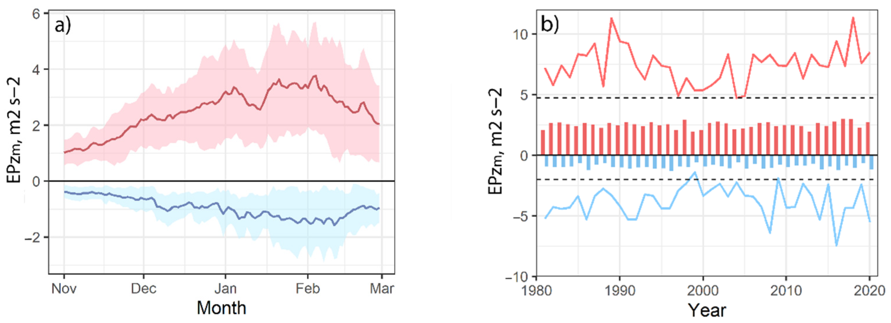
WAFs are very weak in October and start to intensify when the polar night sets in and strong radiative cooling speeds up. From the beginning of November, WAFs are strong enough to penetrate the stratosphere and influence its radiative equilibrium. Nonetheless, November is a month with relatively low WAF intensity and with very little variance in EPzm values (see Table 1). Extremely high ↑EPzm values were recorded at the end of November and during the beginning of December only in 1987–1988, 1993–1994, 1997–1998, and 2008–2009. These cases can be considered as representing very early upward WAF anomalies, because WAFs intensify during the winter and the most anomalous values are usually registered during late DJF season (Figure 1a). This is also related to the evolution and activity of planetary waves of tropospheric origin and their accumulative influence on the stratosphere. For December, ↑EPzm values significantly increase but ↓EPzm is quite low, indicating that upward propagation suddenly begins to strengthen, while downward propagation remains weak. The first climatological minor peak of ↑EPzm can be observed at the beginning of January and the main peak of ↑EPzm around 4 February. Meanwhile ↓EPzm decreases throughout the cold season, reaching its lowest values around 11 February. The climatological daily values of EPzm WAFs are illustrated in Figure 1a, where the shadowed regions indicate daily standard deviations. The average time lag between the peaks of ↑EPzm and ↓EPzm is about one week. This time interval can be considered as the time of the strongest “troposphere stratosphere troposphere” coupling.
The average EPzm values for the entire period of November–February are 2.4 m2s−2 for a ↑EPzm and −1.4 m2s−2 for a ↓EPzm. These values do not vary much from season to season (even considering only the DJF season) and are very far from the EPzm extremes (EPze) (Figure 1b). Over the last four decades ↑EPzm values varied from 0 to 11.3 m2s−2 (the absolute maximum was registered in 2018 in the Canadian region, see Section 3.4), while ↓EPzm values had a diapason of −7.4 0 m2s−2 (the absolute minimum was registered in 2016 in the Canadian–Greenland region, see Section 3.4). The highest ↑EPzm and the lowest ↓EPzm monthly average values were found in January, while the absolute extremes were identified in February. The average values and absolute extremes for each month and their standard deviations are listed in Table 1.
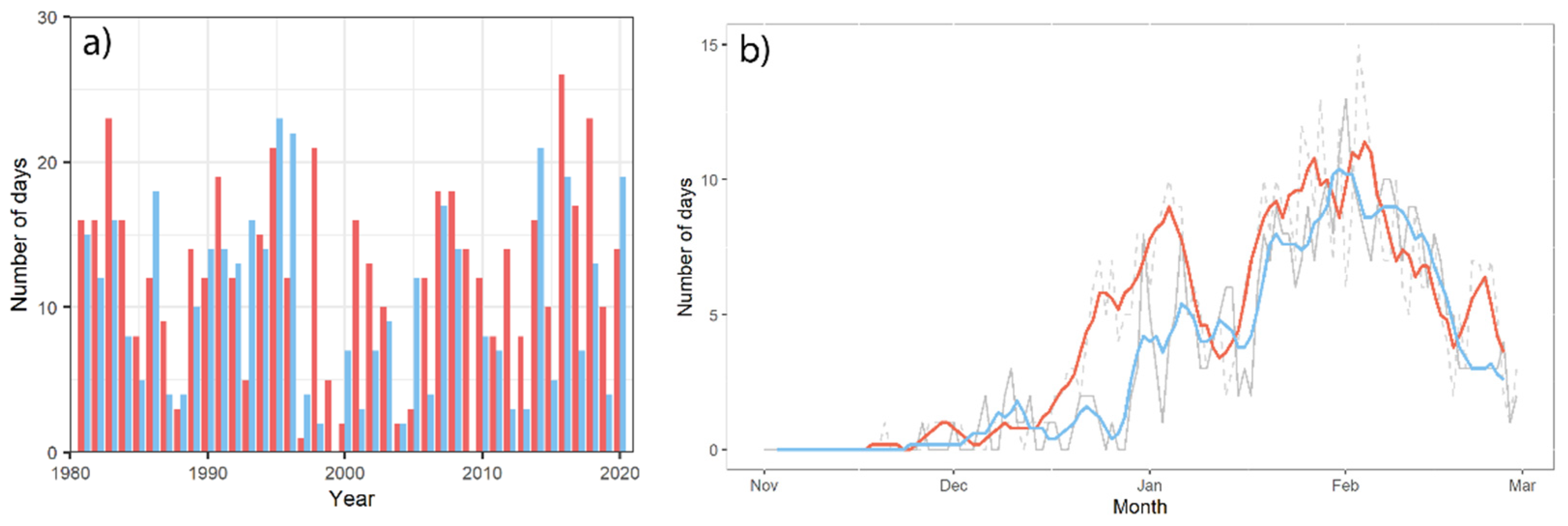
To evaluate most the extreme events of EPzm, the 10th and 90th percentiles were used as the threshold for downward and upward EPze, respectively. The calculated critical values are 4.7 m2s−2 for ↑EPzm and −2.0 m2s−2 for ↓EPzm. Above and below these values, EPz WAFs can be considered as extremely anomalous and sufficient to make some changes in existing thermodynamic conditions: to provoke the SSW in the stratosphere or penetrate down to the troposphere. On average, there were about 11 days with extremely anomalous ↑EPze values every NDJF season, but certain years had no such values, or only 1–2 days per season (e.g., 1987–1988, 1996–1997, 1999–2000, 2003–2004, and 2004–2005). For a ↓EPze, the average for a season was 9 days, but again, in several years WAFs did not reach extremely high values (e.g., 1998–1999, 2008–2009). Other years could have had 20 or more days with extreme ↓EPze values (e.g., 1994–1995, 1995–1996, 2013–2014). The interannual variability of the number of days, separately for upward and downward EPze is shown in Figure 2a.
During the NDJF season, ↑EPze had two peaks of frequency (Figure 2b): a minor peak was registered in the beginning of January and a major one at the end of January–beginning of February. These peaks show the highest probability of an anomalous high EPze during the NDJF with the most likely time for the occurrence of SSW. The frequencies of ↑EPze and ↓EPze were seen almost simultaneously.
3.2. EPz WAF Tendencies over the Last 40 Years
The tendencies of EPzm variability were determined using monthly and seasonally (NDJF) averaged data. According to the Mann–Kendall test, no statistically significant changes were found. According to the test a slightly positive (0.03 m2 s−2 per decade) tendency of ↑EPzm in 1981–2020 existed, while ↓EPzm values experienced a weak decrease (–0.02 m2 s−2 per decade). The largest increase in ↑EPzm intensity was found in January, while slight negative regression coefficients were obtained for December and February. ↓EPzm showed a decreasing tendency in all months, except February.
Analysing the variation of the number of days with EPze, a negligible (1 day per 100 years) increase in the number of days with ↑EPze was determined. These changes were accompanied by an increase in the absolute seasonal maximum of ↑EPz of 0.15 m2 s−2 per decade. A slightly larger decrease was found in the number of days with ↓EPze (3 days per 100 years), but with no changes in the absolute seasonal minimum of ↓EPz.
The results show little or no changes in the strength of upward and downward wave activity flux over past 40 years. Changes in extreme anomalous WAFs were also minor.
3.3. Statistical Relationships between EPzm and Stratospheric Temperature Anomalies
The statistical relationships between ↑EPzm and stratospheric zonal mean temperature (10 hPa level, averaged around the polar cap 60–90 °N) anomalies were evaluated using daily time series for every NDJF separately during 1981–2020. Stratospheric temperature anomalies were calculated subtracting the long-term (1979–2020) mean from each day. A time-lagged cross-correlation analysis was used for each year and the time series were shifted relatively in time. Finally, the mean lag for maximum correlation was evaluated.
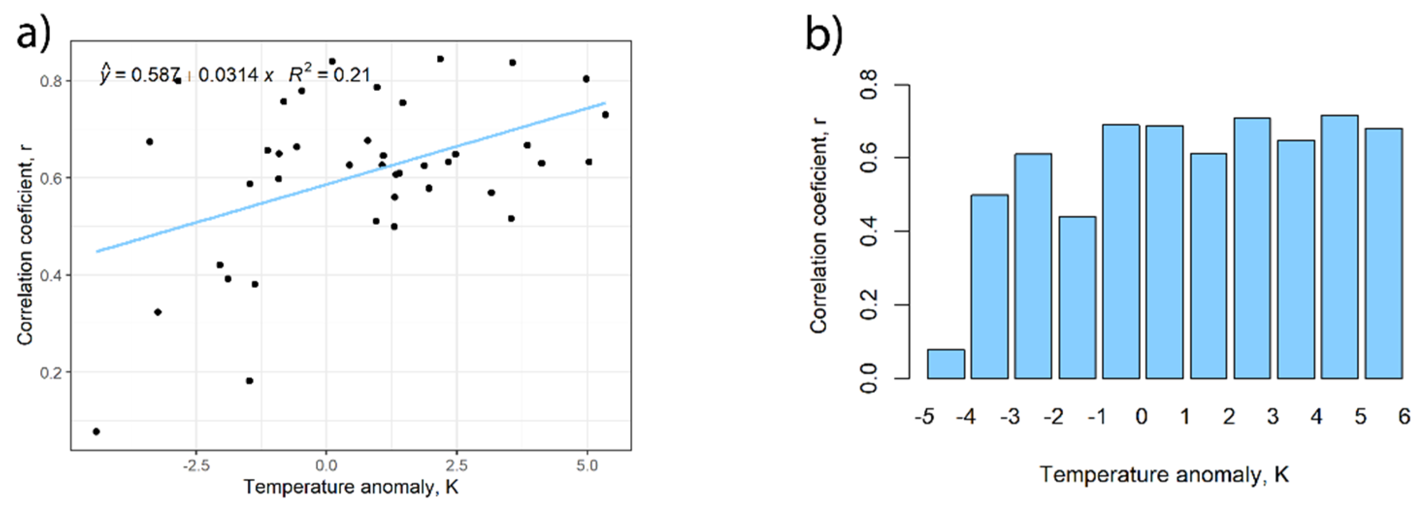
There was a very high coincidence between the two parameters with a minor time- lag. On average, this time lag was 2.8 days (ranging from one to seven days) with SD = 1.5 (not shown). This means that the stratospheric temperature on average increases 2.8 days after upward EPzm is increased. Pearson’s correlation coefficient r, calculated for each year separately, ranged from 0.08 to 0.84 (Figure 3a). It should be noted that in 17% of all years r < 0.5, which means that even if the vertical WAF is proportional to the meridional heat flux, the strength of the relationship between ↑EPzm and stratospheric in some years can be quite weak.
Only one value fell below a 95% significance level (which is 0.18 for the number of observations N = 120), calculated for the 1996–1997 NDJF season. This season can be characterised as the season with the coldest stratosphere during the investigation period (anomaly is −4.4 K). Moreover, a very weak, but statistically significant relation was determined for the season of 2004–2005 with a correlation coefficient of 0.18 (Figure 3a). This season was also colder than usual (anomaly is −1.5 K). Our more detailed analysis showed that the weakest relationships between the analysed parameters were determined during the cold stratosphere NDJF seasons (Figure 3b), which implies that the initial condition of the stratosphere plays an important role in the further evolution of the SSW.
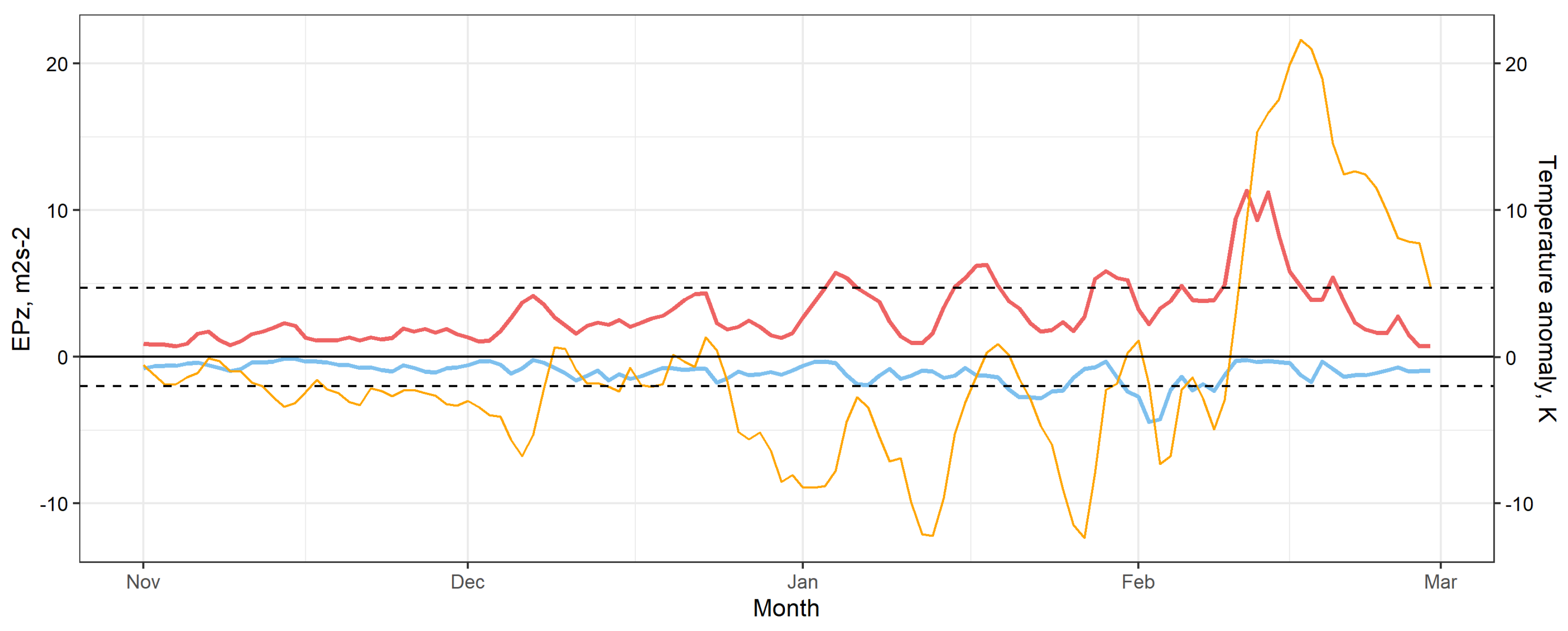
When the temperature in the stratosphere is low enough for a quite long period of time (more than 30 days), at least two ↑EPze pulses over a short time interval (two weeks or less) are usually needed to raise polar temperatures significantly. It should be mentioned that negative temperature anomalies at the 10-hPa level have occurred more often in recent decades (a statistically significant trend equal to −0.07 degree per NDJF in 1981–2020). The obtained result is in a good agreement with the results of other studies [56,57], which also found stratosphere cooling during the last decades. For example, in the study by Steiner et al. [56], using merged operational satellite measurements, radiosondes, lidars, and RO data, the robust cooling of the stratosphere of about 1–3 K during the 1979–2018 was established. The calculated trend in this study falls within this range. Along with a cooling stratosphere, it is possible that in the future more than one extremely intensive EPze pulse will often be needed for the evolution of the stratospheric anomalies. A good example could be the one of the last major SSW, which was recorded on 11 February, 2018. The NDJF season of 2017–2018 can be also described as a cold stratosphere year, when the SSW took place only along with the fourth ↑EPze (Figure 4). A very similar situation was observed before the major SSWs in 2016 and 2008.
The correlation coefficient between the ↑EPzm and stratosphere polar cap temperature anomaly in 2017–2018 was equal to 0.73. It can be seen from Figure 4 that each of the first three ↑EPze fluxes rose polar temperatures, but not enough to cause a SSW. After the first two ↑EPze fluxes, the temperatures dropped back to the previous values. For this reason, it would not be entirely correct to call the influence of ↑EPze accumulative. The major SSW was registered only after the last ↑EPze on 11 February, 2018, with ↑EPz 11.3 m2s−2 (shown in Figure 5e), and this was the absolute ↑EPz maximum over the last four decades. Over the space of a few days, the stratospheric temperatures increased by more than 20 K and a reversal of the westerly winds occurred.
However, more importantly, significant ↓EPze (Figure 5b,d) were registered only after the second (Figure 5a) and third ↑EPze (Figure 5c), and no ↓EPze was observed after the final ↑EPze (Figure 5f). Previous research has shown that stratospheric states can be distinguished into reflective and non-reflective states [58]. Accordingly, the reflected state means that WAF is reflected back down to the troposphere and affects the structure of the tropospheric planetary waves, and the non-reflective one occurs when WAF is trapped in the stratosphere.
Significant ↓EPze were observed on 20 January and 2 February 2018. These ↓EPz can be traced down to the troposphere (see Figure 5b,d) while during and after the SSW no ↓EPze were found (Figure 5f). This is not a unique phenomenon, but it still requires more attention, namely by addressing issues related to stratosphere troposphere interactions. The comparison of different parameters, describing downward WAF propagation (in our study ↓EPze and the wave reflective index in a study [18]) revealed that both parameters show the same phenomenon and are related with a wave WN1 and WN2 reflection in the upper stratosphere, when the mean zonal wind is substantially weakened.
3.4. Geographical Characteristics of EPzm
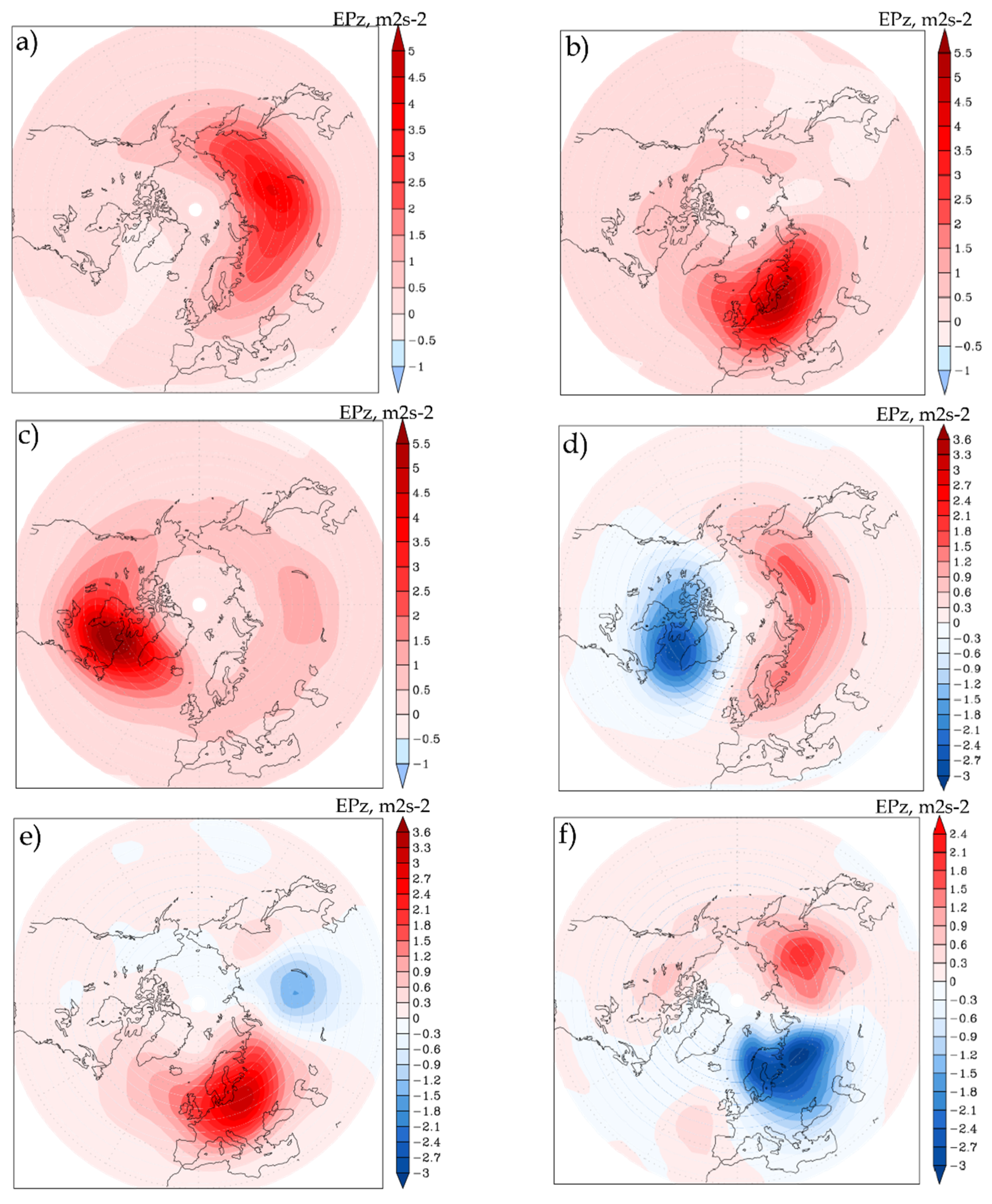
Upward and downward propagating WAFs have different spatial patterns, so-called “zones of influence”. A further classification was made using only EPze values, which, as mentioned above, are most important in “troposphere–stratosphere troposphere” interactions. Our analysis showed that 59% of all analysed ↑EPze cases were found over the Asian region and 26% over the European region; only 15% were observed over the North America–North Atlantic region (corresponding to Figure 6a–c). ↓EPze usually (69%) occurred over the North America–North Atlantic (more precisely over Canadian–Greenland region) and the European region (18%), while over the Asian region, they were only rarely recorded (13%) (corresponding to Figure 6d–f).
These results confirm the findings of Ke and Wen; Zyulyaeva and Zhadin; Ke et al.; and Jadin [34,35,36,59], who showed that upward and downward wave fluxes have their own regions of occurrence. Upward propagation takes place over Northern Eurasia and downward WAFs are usually found over North America and the North Atlantic region (NANA region). This pattern was named a “stratospheric wave bridge” and the downward propagation region was described as a stratospheric “wave hole”, where the wave energy from the stratosphere can potentially penetrate the troposphere. The seasonal absolute maxima and minima of EPzm were used to illustrate these features. The maps (Figure 6) illustrate the most common spatial patterns of extreme upward and downward WAFs. The so-called “stratospheric bridge”, which forms due to the reflection of a zonally propagating wave packet, can be seen in Figure 6d–f. As shown in the pictures, the locations of extreme EPzs vary a lot from season-to-season and could be one of the key indicators for improving regional long-term forecasts of severe weather events.
4. Summary and Conclusions
This study investigated the vertical component of EP WAF (EPzm), which is a key indicator of the upward and downward propagation of planetary-scale waves and, according to previous studies, may be a useful precursor to SSW and later for tropospheric anomalies.
The results obtained in the first part of the analysis suggest that EPz values, averaged over a long time period, mask a lot of useful information. The same may apply to the spatial averaging over broad latitudinal belts or even for all of the NH. Therefore, only daily maxima and minima (EPzm) were used in this study. When the extreme values are used, there may be a risk of involving small number statistics. For this reason, daily values were used and the non-parametric Mann–Kendall test was applied.
Firstly, the main climatological characteristics of EPzm fluxes were established. The analysis showed that WAFs intensify during the winter and that most anomalous values are usually recorded in the second half of the cold season with a peak around 4 February for upward propagating WAFs and the 11 February for downward propagating WAFs. These peaks coincide well with the peaks of reoccurrence of EPze. A minor peak was distinguished at the beginning of January and a major one at the end of January–beginning of February.
It was observed that after an anomalous strong upward EPz, which is around 4.7 m2s−2 or more, a more intensive downward EPz can usually be expected. The time lag between upward and downward EPze is only a few days. Moreover, an anomalous strong EPz has a noticeable vertical extension. During the extreme cases, ↑EPz flux was detected several days before in the troposphere, but further eastward than the stratospheric maximum and the later ↓EPz flux was traced down to the tropopause (9–12 km height) within the next several days. These results confirm that the magnitude of EPz is a very important feature, which determines the extent of vertical propagation and may initiate further changes in thermodynamical characteristics. This applies to both the stratosphere and the troposphere.
The statistical relationships between ↑EPzm and stratospheric temperature anomalies were evaluated. It can be concluded that there is a very high coincidence between these two parameters with an average time lag of 2.8 days. The weakest relationships between ↑EPzm and stratospheric temperatures were recognised during the colder than usual stratosphere NDJF seasons. This indicates that the general condition of the stratosphere is an important factor. If the ↑EPzm is weak during November–December, the stratosphere temperature can decrease sufficiently and two or more strong ↑EPze pulses with short time intervals (two weeks or less) are usually needed for the formation of a SSW; for example, this was observed before the SSW in 2018. In conclusion, not every EPze can cause a SSW, but every EPze has some influence on the stratospheric temperature fluctuations.
Considering the influence of the stratosphere on the troposphere, a very important feature of wave fluxes is their downward propagation. It seems that ↓EPzm is related to a wave WN1 and WN2 reflection in the upper stratosphere. The study [18] showed that downward reflected waves were responsible for the formation of a deep trough over Eurasia and caused extreme cold weather conditions in mid-January 2013. The wave reflective index proposed in [2] was used in their analysis, and this index corresponds well with the downward EPze presented in this study. This makes the extreme events more predictable, but it is still unknown which region can be affected. Moreover, the review of the SSW in 2018 in this analysis revealed that even after a major SSW, the downward EPzm was not sufficiently strong; this is one of the issues that should receive more attention in the future.
Another important characteristic of the WAFs is the dominant spatial pattern of EPzm. Upward and downward propagating WAFs have different “areas of influence”. ↑EPze are usually observed over the Asian region and ↓EPze are more pronounced over the North America North Atlantic (NANA) region. This bipolar phenomenon was called a “stratospheric bridge” in the previous studies [34,35,59]. However, the “stratospheric bridge” does not always act as it has been described before. During certain years, we can observe this bipolar phenomenon over Asia–Europe and in other years in the opposite direction over Europe–Asia, bypassing the NANA region. Further research is needed to determine if this has a significant impact on the occurrence of surface weather anomalies. It is possible that the region and magnitude of reflected downward WAFs could be some of decisive factors affecting the location and severity of the tropospheric anomalies.
Moreover, the results of this study reveal that despite the rapidly changing climate of the last decades, there were no statistically significant changes in the intensity and duration (number of days) of EPzm. Thus, the wave flux energy propagating with WN1 and WN2 type waves may have a very similar effect on the stratosphere and its thermodynamic processes in the future. Another question that needs answering is to what extent the signal coming from the stratosphere will be able to influence the tropospheric weather regime, due to the changing state of the troposphere itself.
Answering these questions may significantly contribute to our understanding of the importance of EPze to the formation of surface temperature anomalies.
Funding
This research was funded by European Social Fund under grant agreement with the Re-search Council of Lithuania (LMTLT) [grant number 09.3.3-LMT-K-712-02-0141].
Institutional Review Board Statement
Not applicable.
Informed Consent Statement
Not applicable.
Data Availability Statement
MERRA-2 reanalysis data are available online via NASA’s Goddard Earth Sciences Data and Information Services Center archive (https://gmao.gsfc.nasa.gov/reanalysis/MERRA-2/data_access/ (accessed on 10 July 2021)).
Acknowledgments
I thank NASA for making the MERRA2 reanalysis data available. I thank professors E. Rimkus (Vilnius University, Lithuania) and A.I. Pogoreltsev (Russian State Hydrometeorological University) for their help with this research, and the anonymous reviewers for their very constructive comments that improved this study.
Conflicts of Interest
The authors declare no conflict of interest.
Abbreviations
| ↑EPzm | maximum of the upward vertical component of Eliassen–Palm wave activity flux; |
| ↓EPzm | minimum of the downward vertical component of Eliassen–Palm wave activity flux; |
| ↑EPze | 90th percentile of the maximum of the upward vertical component of Eliassen–Palm wave activity flux; |
| ↓EPze | 10th percentile of the minimum of the downward vertical component of Eliassen–Palm wave activity flux. |
References
- Baldwin, M.P.; Dunkerton, T.J. Propagation of the Arctic Oscillation from the stratosphere to the troposphere. J. Geophys. Res. 1999, 104, 30937–30946. [Google Scholar] [CrossRef]
- Perlwitz, J.; Harnik, N. Downward coupling between the stratosphere and troposphere: The relative roles of wave and zonal mean processes. J. Clim. 2004, 17, 4902–4909. [Google Scholar] [CrossRef] [Green Version]
- Kodera, K.; Mukougawa, H.; Itoh, S. Tropospheric impact of reflected planetary waves from the stratosphere. Geophys. Res. Lett. 2008, 35, L16806. [Google Scholar] [CrossRef]
- Cohen, J.; Screen, J.A.; Furtado, J.C.; Barlow, M.; Whittleston, D.; Coumou, D.; Francis, J.; Dethloff, K.; Entekhabi, D.; Overland, J.; et al. Recent Arctic amplification and extreme mid-latitude weather. Nat. Geosci. 2014, 7, 627–637. [Google Scholar] [CrossRef] [Green Version]
- Kidston, J.; Scaife, A.; Hardiman, S.; Mitchell, D.M.; Butchart, N.; Baldwin, M.P.; Gray, L.J. Stratospheric influence on tropospheric jet streams, storm tracks and surface weather. Nat. Geosci. 2015, 8, 433–440. [Google Scholar] [CrossRef]
- Cai, M.; Yu, Y.; Deng, Y.; van den Dool, H.M.; Ren, R.; Saha, S.; Wu, X.; Huang, J. Feeling the Pulse of the Stratosphere: An Emerging Opportunity for Predicting Continental-Scale Cold-Air Outbreaks 1 Month in Advance. Bull. Am. Meteorol. Soc. 2016, 97, 1475–1489. [Google Scholar] [CrossRef]
- Karpechko, A.Y.; Hitchcock, P.; Peters, D.H.W.; Schneidereit, A. Predictability of downward propagation of major sudden stratospheric warmings. Q. J. R. Meteorol. Soc. 2017, 143, 1459–1470. [Google Scholar] [CrossRef]
- Kretschmer, M.; Coumou, D.; Agel, L.; Barlow, M.; Tziperman, E.; Cohen, J. More-Persistent Weak Stratospheric Polar Vortex States Linked to Cold Extremes. Bull. Am. Meteor. Soc. 2018, 99, 49–60. [Google Scholar] [CrossRef]
- Kretschmer, M.; Cohen, J.; Matthias, V.; Runge, J.; Coumou, D. The different stratospheric influence on cold-extremes in Eurasia and North America. NPJ Clim. Atmos. Sci. 2014, 1, 44. [Google Scholar] [CrossRef] [Green Version]
- Lee, S.H.; Charlton-Perez, A.J.; Furtado, J.C.; Woolnough, S.J. Abrupt stratospheric vortex weakening associated with North Atlantic anticyclonic wave breaking. J. Geophys. Res. Atmos. 2019, 124, 8563–8575. [Google Scholar] [CrossRef] [Green Version]
- Zhou, X.; Chen, Q.; Wang, Z.; Xu, M.; Zhao, S.; Cheng, Z.; Feng, F. Longer Duration of the Weak Stratospheric Vortex During Extreme El Nino Events Linked to Spring Eurasian Coldness. J. Geophys. Res. Atmos. 2020, 125, e2019JD032331. [Google Scholar] [CrossRef]
- Cagnazzo, C.; Manzini, E.; Calvo, N.; Douglass, A.; Akiyoshi, H.; Bekki, S.; Chipperfield, M.; Dameris, M.; Deushi, M.; Fischer, A.M.; et al. Northern winter stratospheric temperature and ozone responses to ENSO inferred from an ensemble of Chemistry Climate Models. Atmos. Chem. Phys. 2009, 9, 8935–8948. [Google Scholar] [CrossRef] [Green Version]
- Xie, F.; Li, J.; Tian, W.; Feng, J.; Huo, Y. The Signals of El Niño Modoki in the Tropical Tropopause Layer and Stratosphere. Atmos. Chem. Phys. 2012, 12, 5259–5273. [Google Scholar] [CrossRef] [Green Version]
- Garfinkel, C.I.; Hartmann, D.L. Effects of El Nino—Southern Oscillation and the Quasi-Biennial Oscillation on polar temperatures in the stratosphere. J. Geophys. Res. 2007, 112, D19112. [Google Scholar] [CrossRef] [Green Version]
- Charlton, A.; Polvani, L. A new look at stratospheric sudden warmings. Part I: Climatology and modeling benchmarks. J. Clim. 2007, 20, 449–469. [Google Scholar] [CrossRef]
- Tripathi, O.P.; Baldwin, M.; Charlton-Perez, A.; Charron, M.; Cheung, J.C.H.; Eckermann, S.D.; Gerber, E.; Jackson, D.R.; Kuroda, Y.; Lang, A.; et al. Examining the Predictability of the Stratospheric Sudden Warming of January 2013 Using Multiple NWP Systems. Mon. Weather Rev. 2016, 144, 1935–1960. [Google Scholar] [CrossRef] [Green Version]
- Jucker, M.; Reichler, T. Dynamical precursors for statistical prediction of stratospheric sudden warming events. Geophys. Res. Lett. 2018, 45, 13–124. [Google Scholar] [CrossRef]
- Nath, D.; Chen, W.; Zelin, C.; Pogoreltsev, A.I.; Wei, K. Dynamics of 2013 Sudden Stratospheric Warming event and its impact on cold weather over Eurasia: Role of planetary wave reflection. Sci. Rep. 2016, 6, 24174. [Google Scholar] [CrossRef] [PubMed]
- Thuburn, J.; Craig, G.C. Stratospheric Influence on Tropopause Height: The Radiative Constraint. J. Atmos. Sci. 2000, 57, 17–28. [Google Scholar] [CrossRef]
- Karpechko, A.Y.; Charlton-Perez, A.; Balmaseda, M.; Tyrrell, N.; Vitart, F. Predicting sudden stratospheric warming 2018 and its climate impacts with a multimodel ensemble. Geophys. Res. Lett. 2018, 45, 13538–13546. [Google Scholar] [CrossRef] [Green Version]
- Polvani, L.M.; Waugh, D.W. Upward Wave Activity Flux as a Precursor to Extreme Stratospheric Events and Subsequent Anomalous Surface Weather Regimes. J. Clim. 2004, 17, 3548–3554. [Google Scholar] [CrossRef]
- Jaiser, R.; Dethloff, K.; Handorf, D. Stratospheric response to Arctic sea ice retreat and associated planetary wave propagation change. Tellus A Dyn. Meteorol. Oceanogr. 2013, 65, 1. [Google Scholar] [CrossRef] [Green Version]
- Solomon, A. Wave Activity Events and the Variability of the Stratospheric Polar Vortex. J. Clim. 2014, 27, 7796–7806. [Google Scholar] [CrossRef]
- Martineau, P.; Chen, G.; Son, S.-W.; Kim, J. Lower-stratospheric control of the frequency of sudden stratospheric warming events. J. Geophys. Res. Atmos. 2018, 123, 3051–3070. [Google Scholar] [CrossRef]
- Martineau, P.; Son, S. Onset of Circulation Anomalies during Stratospheric Vortex Weakening Events: The Role of Planetary-Scale Waves. J. Clim. 2015, 28, 7347–7370. [Google Scholar] [CrossRef]
- Nakagawa, K.I.; Yamazaki, K. What kind of stratospheric sudden warming propagates to the troposphere? Geophys. Res. Lett. 2006, 33, L04801. [Google Scholar] [CrossRef] [Green Version]
- Rao, J.; Garfinkel, C.I.; White, I.P. Predicting the downward and surface influence of the February 2018 and January 2019 sudden stratospheric warming events in subseasonal to seasonal (S2S) models. J. Geophys. Res. Atmos. 2020, 125, e2019JD031919. [Google Scholar] [CrossRef] [Green Version]
- Lee, S.H.; Furtado, J.C.; Charlton-Perez, A.J. Wintertime North American weather regimes and the Arctic stratospheric polar vortex. Geophys. Res. Lett. 2019, 46, 14892–14900. [Google Scholar] [CrossRef]
- Polvani, L.M.; Sun, L.; Butler, A.H.; Richter, J.H.; Deser, C. Distinguishing Stratospheric Sudden Warmings from ENSO as Key Drivers of Wintertime Climate Variability over the North Atlantic and Eurasia. J. Clim. 2017, 30, 1959–1969. [Google Scholar] [CrossRef]
- Butler, A.H.; Sjoberg, J.P.; Seidel, D.J.; Rosenlof, K.H. A sudden stratospheric warming compendium. Earth Syst. Sci. Data 2017, 9, 63–76. [Google Scholar] [CrossRef] [Green Version]
- King, A.D.; Butler, A.H.; Jucker, M.; Earl, N.O.; Rudeva, I. Observed relationships between sudden stratospheric warmings and European climate extremes. J. Geophys. Res. Atmos. 2019, 124, 13943–13961. [Google Scholar] [CrossRef]
- Domeisen, D.I.V.; Grams, C.M.; Papritz, L. The role of North Atlantic–European weather regimes in the surface impact of sudden stratospheric warming events. Weather Clim. Dynam. 2020, 1, 373–388. [Google Scholar] [CrossRef]
- Overland, J.; Hall, R.; Hanna, E.; Karpechko, A.; Vihma, T.; Wang, M.; Zhang, X. The Polar Vortex and Extreme Weather: The Beast from the East in Winter 2018. Atmosphere 2020, 11, 664. [Google Scholar] [CrossRef]
- Ke, W.; Wen, C. Northern Hemisphere Stratospheric Polar Vortex Extremes in February under the Control of Downward Wave Flux in the Lower Stratosphere. Atmos. Ocean. Sci. Lett. 2012, 5, 183–188. [Google Scholar] [CrossRef]
- Zyulyaeva, Y.A.; Zhadin, E.A. Analysis of three-dimensional Eliassen-Palm fluxes in the lower stratosphere. Russian Meteor. Hydrol. 2009, 34, 483–490. [Google Scholar] [CrossRef]
- Wei, K.; Ma, J.; Chen, W.; Vargin, P. Longitudinal peculiarities of planetary waves-zonal flow interactions and their role in stratosphere-troposphere dynamical coupling. Clim. Dyn. 2021, 1–20. [Google Scholar] [CrossRef]
- Plumb, R.A. On the three-dimensional propagation of stationary waves. J. Atmos. Sci. 1985, 42, 217–229. [Google Scholar] [CrossRef]
- Fletcher, C.G.; Kushner, P.J.; Cohen, J. Stratospheric control of the extratropical circulation response to surface forcing. Geophys. Res. Lett. 2007, 34, L21802. [Google Scholar] [CrossRef]
- Takaya, K.; Nakamura, H. A Formulation of a Phase-Independent Wave-Activity Flux for Stationary and Migratory Quasigeostrophic Eddies on a Zonally Varying Basic Flow. J. Atmos. Sci. 2001, 58, 608–627. [Google Scholar] [CrossRef]
- Domeisen, D.I.V.; Martius, O.; Jiménez-Esteve, B. Rossby wave propagation into the Northern Hemisphere stratosphere: The role of zonal phase speed. Geophys. Res. Lett. 2018, 45, 2064–2071. [Google Scholar] [CrossRef] [Green Version]
- Sussman, H.S.; Raghavendra, A.; Roundy, P.E.; Dai, A. Trends in northern midlatitude atmospheric wave power from 1950 to 2099. Clim. Dyn. 2020, 54, 2903–2918. [Google Scholar] [CrossRef]
- Cohen, J.; Furtado, J.C.; Jones, J.; Barlow, M.; Whittleston, D.; Entekhabi, D. Linking Siberian Snow Cover to Precursors of Stratospheric Variability. J. Clim. 2014, 27, 5422–5432. [Google Scholar] [CrossRef]
- Petoukhov, V.; Semenov, V.A. A link between reduced Barents-Kara sea ice and cold winter extremes over northern continents. J. Geophys. Res. 2010, 115, D21111. [Google Scholar] [CrossRef]
- Peings, Y. Ural blocking as a driver of early-winter stratospheric warmings. Geophys. Res. Lett. 2019, 46, 5460–5468. [Google Scholar] [CrossRef]
- Garfinkel, C.I.; Hartmann, D.L.; Sassi, F. Tropospheric Precursors of Anomalous Northern Hemisphere Stratospheric Polar Vortices. J. Clim. 2010, 23, 3282–3299. [Google Scholar] [CrossRef]
- Zhang, R.; Tian, W.; Wang, T. Role of the quasi-biennial oscillation in the downward extension of stratospheric northern annular mode anomalies. Clim. Dyn. 2020, 55, 595–612. [Google Scholar] [CrossRef]
- Petoukhov, V.; Rahmstorf, S.; Petri, S.; Schellnhuber, H.J. Quasiresonant amplification of planetary waves and recent Northern Hemisphere weather extremes. Proc. Natl. Acad. Sci. USA 2013, 110, 5336–5341. [Google Scholar] [CrossRef] [Green Version]
- Dee, D.P.; Uppala, S.M.; Simmons, A.J.; Berrisford, P.; Poli, P.; Kobayashi, S.; Andrae, U.; Balmaseda, M.A.; Balsamo, G.; Bauer, P.; et al. The ERA-Interim reanalysis: Configuration and performance of the data assimilation system. Q. J. R. Meteorol. Soc. 2011, 137, 553–597. [Google Scholar] [CrossRef]
- Uppala, S.M.; Kållberg, P.W.; Simmons, A.J.; Andrae, U.; da Costa Bechtold, V.; Fiorino, M.; Gibson, J.K.; Haseler, J.; Hernandez, A.; Kelly, G.A.; et al. The ERA-40 re-analysis. Q. J. R. Meteorol. Soc. 2005, 131, 2961–3012. [Google Scholar] [CrossRef]
- Kistler, R.; Collins, W.; Saha, S.; White, G.; Woollen, J.; Kalnay, E.; Chelliah, M.; Ebisuzaki, W.; Kanamitsu, M.; Kousky, V.; et al. The NCEP–NCAR 50-year reanalysis: Monthly means CD-ROM and documentation. Bull. Am. Meteorol. Soc. 2001, 82, 247–267. [Google Scholar] [CrossRef]
- Gelaro, R.; McCarty, W.; Suárez, M.J.; Todling, R.; Molod, A.; Takacs, L.; Randles, C.A.; Darmenov, A.; Bosilovich, M.G.; Reichle, R.; et al. The Modern-Era Retrospective Analysis for Research and Applications, Version 2 (MERRA-2). J. Clim. 2017, 30, 5419–5454. [Google Scholar] [CrossRef] [PubMed]
- Wargan, K.; Coy, L. Strengthening of the Tropopause Inversion Layer during the 2009 Sudden Stratospheric Warming: A MERRA-2 Study. J. Atmos. Sci. 2016, 73, 1871–1887. [Google Scholar] [CrossRef]
- Huang, C.; Li, W.; Zhang, S.; Chen, G.; Huang, K.; Gong, Y.; Dai, A. Investigation of dominant traveling 10-day wave components using long-term MERRA-2 database. Earth Planets Space 2021, 73, 85. [Google Scholar] [CrossRef]
- Coy, L.; Newman, P.A.; Pawson, S.; Lait, L.R. Dynamics of the Disrupted 2015-16 Quasi-Biennial Oscillation. J. Clim. 2017, 30, 5661–5674. [Google Scholar] [CrossRef]
- Attard, H.E.; Lang, A.L. Troposphere–Stratosphere Coupling Following Tropospheric Blocking and Extratropical Cyclones. Mon. Weather Rev. 2019, 147, 1781–1804. [Google Scholar] [CrossRef]
- Steiner, A.K.; Ladstädter, F.; Randel, W.J.; Maycock, A.C.; Fu, Q.; Claud, C.; Gleisner, H.; Haimberger, L.; Ho, S.-P.; Keckhut, P.; et al. Observed Temperature Changes in the Troposphere and Stratosphere from 1979 to 2018. J. Clim. 2020, 33, 8165–8194. [Google Scholar] [CrossRef]
- Karpechko, A.Y.; Maycock, A.C.; Abalos, M.; Akiyoshi, H.; Arblaster, J.M.; Garfinkel, C.I.; Rosenlof, K.H.; Sigmond, M. Stratospheric Ozone Changes and Climate. In Scientific Assessment of Ozone Depletion; Fahey, D.W., Newman, P.A., Pyle, J.A., Safari, B., Eds.; World Meteorological Organization: Geneva, Switzerland, 2018; Volume 58. [Google Scholar]
- Perlwitz, J.; Harnik, N. Observational evidence of a stratospheric influence on the troposphere by planetary wave reflection. J. Clim. 2003, 16, 3011–3026. [Google Scholar] [CrossRef]
- Jadin, E.A. Stratospheric “wave hole” and interannual variations of the stratospheric circulation in late winter. Nat. Sci. 2011, 3, 259–267. [Google Scholar] [CrossRef] [Green Version]
Figure 1.
Climatology of EPzm WAF; (a) daily variability of upward EPzm (red line) and downward EPzm (blue line) averaged over 1981–2020, where shadowed ribbons show the standard deviation for each day; (b) average NDJF values of upward EPzm (red bars), downward EPzm (blue bars), and absolute seasonal EPzm maxima (red line) and minima (blue line) over 1981–2020. The dashed horizontal lines accordingly show the 90th and 10th percentiles of ↑EPzm and ↓EPzm.

Figure 2.
The variability of the total number of days with EPze: (a) interannual variability (red bars indicate upward EPze and blue bars downward EPze) and (b) intra-seasonal variability (the grey dashed line shows upward EPze and the red line indicates a 5-day moving average. The grey solid line shows downward EPze and the blue line indicates a 5-day moving average), 1981–2020 NDJF.

Figure 3.
The scatter plot with regression line (a) shows the magnitude of the Pearson’s correlation coefficient between ↑EPzm (30km), and the polar cap air temperature at 10 hPa vs the mean NDJF temperature (10 hPa, 60–90 °N) anomaly (K) for each year; and histogram (b) shows the distribution of averaged correlation coefficient within different stratosphere temperature (10 hPa, 60–90 °N) anomaly (K) intervals.

Figure 4.
Upward (red solid line) and downward (blue solid line) EPzm and stratosphere polar cap temperature anomaly (yellow solid line) during the 2018 NDJF (year of the major SSW); the dashed horizontal lines show accordingly the 90th and 10th percentiles of EPzm.
Figure 4.
Upward (red solid line) and downward (blue solid line) EPzm and stratosphere polar cap temperature anomaly (yellow solid line) during the 2018 NDJF (year of the major SSW); the dashed horizontal lines show accordingly the 90th and 10th percentiles of EPzm.

Figure 5.
Longitude-height (km) cross section of: (a) EPz before SSW on 18 January, 2018; (b) EPz before SSW on 20 January, 2018; (c) EPz before SSW on 29 January, 2018; (d) EPz before SSW on 2 February, 2018; (e) EPz during SSW on 11 February, 2018; (f) EPz after SSW on 17 February, 2018; averaged at 62.5 °N latitude.

Figure 6.
The dominant spatial patterns of absolute ↑EPzm: (a) Asian, (b) European, (c) Canadian–Greenland; and absolute ↓EPzm, (d) Canadian–Greenland, (e) Asian, (f) European during 1981–2020 in the Northern Hemisphere (30–90 °N) at 30 km height.
Figure 6.
The dominant spatial patterns of absolute ↑EPzm: (a) Asian, (b) European, (c) Canadian–Greenland; and absolute ↓EPzm, (d) Canadian–Greenland, (e) Asian, (f) European during 1981–2020 in the Northern Hemisphere (30–90 °N) at 30 km height.


Table 1.
The average ↑EPzm (left) and ↓EPzm (right) values and their absolute extremes for each month and their standard deviations (SD).
Table 1.
The average ↑EPzm (left) and ↓EPzm (right) values and their absolute extremes for each month and their standard deviations (SD).
| Month | Average ↑EPzm | SD ↑EPzm | Absolute ↑EPzm Monthly Maxima | SD abs. Maxima ↑EPzm | Average ↓EPzm | SD ↓EPzm | Absolute ↓EPzm Monthly Minima | SD abs. Minima ↓EPzm |
|---|---|---|---|---|---|---|---|---|
| November | 1.45 | 0.36 | 5.67 | 1.03 | −0.49 | 0.13 | −2.18 | 0.43 |
| December | 2.51 | 0.64 | 8.33 | 1.43 | −0.87 | 0.19 | −3.37 | 0.58 |
| January | 3.18 | 0.85 | 9.21 | 1.79 | −1.24 | 0.42 | −6.39 | 1.26 |
| February | 2.85 | 1.00 | 11.33 | 2.33 | −1.21 | 0.48 | −7.42 | 1.57 |
| NDJF season | 2.50 | 1.56 | 11.33 | 1.56 | –0.95 | 0.18 | –7.42 | 1.28 |
Publisher’s Note: MDPI stays neutral with regard to jurisdictional claims in published maps and institutional affiliations. |
© 2021 by the author. Licensee MDPI, Basel, Switzerland. This article is an open access article distributed under the terms and conditions of the Creative Commons Attribution (CC BY) license (https://creativecommons.org/licenses/by/4.0/).
Share and Cite
MDPI and ACS Style
Gečaitė, I. Climatology of Three-Dimensional Eliassen–Palm Wave Activity Fluxes in the Northern Hemisphere Stratosphere from 1981 to 2020. Climate 2021, 9, 124. https://0-doi-org.brum.beds.ac.uk/10.3390/cli9080124
AMA Style
Gečaitė I. Climatology of Three-Dimensional Eliassen–Palm Wave Activity Fluxes in the Northern Hemisphere Stratosphere from 1981 to 2020. Climate. 2021; 9(8):124. https://0-doi-org.brum.beds.ac.uk/10.3390/cli9080124
Chicago/Turabian StyleGečaitė, Indrė. 2021. "Climatology of Three-Dimensional Eliassen–Palm Wave Activity Fluxes in the Northern Hemisphere Stratosphere from 1981 to 2020" Climate 9, no. 8: 124. https://0-doi-org.brum.beds.ac.uk/10.3390/cli9080124
Note that from the first issue of 2016, this journal uses article numbers instead of page numbers. See further details here.