Article

Plant Species Richness in Multiyear Wet and Dry Periods in the Chihuahuan Desert

1
SCINet Program for Scientific Computing, US Department of Agriculture, Beltsville, MD 20705, USA
2
Jornada Range Unit, US Department of Agriculture, Las Cruces, NM 88003, USA
3
Jornada Basin Long Term Ecological Research Program, New Mexico State University, Las Cruces, NM 88003, USA
4
School of Life Sciences, Arizona State University, Tempe, AZ 85281, USA
5
School of Sustainability, Arizona State University, Tempe, AZ 85281, USA
6
Global Drylands Center, Arizona State University, Tempe, AZ 85281, USA
7
School of Earth and Space Exploration, Arizona State University, Tempe, AZ 85287, USA
8
School of Sustainable Engineering and the Built Environment, Arizona State University, Tempe, AZ 85287, USA
*
Author to whom correspondence should be addressed.
Submission received: 29 May 2021 / Revised: 1 August 2021 / Accepted: 6 August 2021 / Published: 13 August 2021
(This article belongs to the Special Issue Climate System Uncertainty and Biodiversity Conservation)

Abstract

:
In drylands, most studies of extreme precipitation events examine effects of individual years or short-term events, yet multiyear periods (>3 y) are expected to have larger impacts on ecosystem dynamics. Our goal was to take advantage of a sequence of multiple long-term (4-y) periods (dry, wet, average) that occurred naturally within a 26-y time frame to examine responses of plant species richness to extreme rainfall in grasslands and shrublands of the Chihuahuan Desert. Our hypothesis was that richness would be related to rainfall amount, and similar in periods with similar amounts of rainfall. Breakpoint analyses of water-year precipitation showed five sequential periods (1993–2018): AVG1 (mean = 22 cm/y), DRY1 (mean = 18 cm/y), WET (mean = 30 cm/y), DRY2 (mean = 18 cm/y), and AVG2 (mean = 24 cm/y). Detailed analyses revealed changes in daily and seasonal metrics of precipitation over the course of the study: the amount of nongrowing season precipitation decreased since 1993, and summer growing season precipitation increased through time with a corresponding increase in frequency of extreme rainfall events. This increase in summer rainfall could explain the general loss in C3 species after the wet period at most locations through time. Total species richness in the wet period was among the highest in the five periods, with the deepest average storm depth in the summer and the fewest long duration (>45 day) dry intervals across all seasons. For other species-ecosystem combinations, two richness patterns were observed. Compared to AVG2, AVG1 had lower water-year precipitation yet more C3 species in upland grasslands, creosotebush, and mesquite shrublands, and more C4 perennial grasses in tarbush shrublands. AVG1 also had larger amounts of rainfall and more large storms in fall and spring with higher mean depths of storm and lower mean dry-day interval compared with AVG2. While DRY1 and DRY2 had the same amount of precipitation, DRY2 had more C4 species than DRY1 in creosote bush shrublands, and DRY1 had more C3 species than DRY2 in upland grasslands. Most differences in rainfall between these periods occurred in the summer. Legacy effects were observed for C3 species in upland grasslands where no significant change in richness occurred from DRY1 to WET compared with a 41% loss of species from the WET to DRY2 period. The opposite asymmetry pattern was found for C4 subdominant species in creosote bush and mesquite shrublands, where an increase in richness occurred from DRY1 to WET followed by no change in richness from WET to DRY2. Our results show that understanding plant biodiversity of Chihuahuan Desert landscapes as precipitation continues to change will require daily and seasonal metrics of rainfall within a wet-dry period paradigm, as well as a consideration of species traits (photosynthetic pathways, lifespan, morphologies). Understanding these relationships can provide insights into predicting species-level dynamics in drylands under a changing climate.

1. Introduction

Extreme weather events are becoming more frequent [1], and warmer temperatures are expected to continue to increase leading to extreme rainfall and increases in variability as a result of a combination of increased moisture and weakened circulations [2]. In drylands, these extreme, climate-related events include both anomalously high and low amounts of rainfall that have dramatic, long-lasting impacts on ecosystem dynamics [3,4,5,6,7,8,9,10,11,12]. Many studies have examined ecological impacts of individual year events or have manipulated replicated events across years (e.g., [5,13,14]), yet far fewer studies have assessed effects of events that occur over multiple different types of sequential years (e.g., [15,16,17]). Long-term observations are often needed for the duration of, and beyond, these multiyear events, such as the decade-long drought of the 1930s in the central and southern US that contributed to the ‘Dust Bowl’ [14,18,19]. Multiyear extreme events have the greatest potential to influence the trajectory of ecological systems through changes in landscape-soil template properties, and through direct and indirect effects that result in shifts in species dominance [20,21,22]. Drylands are expected to be particularly sensitive to multiyear sequences of above or below-average amounts of precipitation. Low and variable amounts of rainfall and high temperatures in the growing season interact with soil properties to govern patterns in species dominance and composition in arid and semiarid ecosystems located in dryland regions of the world [23,24,25]. The legacy of an extreme event may also be important: a wet year followed by a dry year has different impacts on ecosystems than a dry year followed by a wet year [26,27]. However, little is known about impacts and legacies of multiyear wet or dry periods on patterns in biodiversity.

1.1. Species Richness Responses

Most of the information about the role of extreme events in ecosystems comes from aboveground net primary production (ANPP) responses to short-term dry events (<4 years) (e.g., [17]), although there are some studies of species abundance responses with a focus on plants in the canopy rather than seeds stored in the soil (e.g., [28]). Many studies in drylands have shown that species abundance in the canopy and ANPP are related [29,30,31]. Thus, studies of ANPP can be used to infer responses by species to extreme climatic events. Across grasslands globally, temporal variability of ANPP decreases as species richness increases [30,31,32,33,34,35,36,37,38]. Variable effects of dry events occur through a reordering of dominant aridity-tolerant species [39] and increases or losses in the relative abundance of rare or subordinate species, either in the canopy or stored in the soil seed bank [40,41]. The dominant aridity-tolerant perennial species show changes in cover or ANPP, but not numbers of species, with a single dry year or pulse of rainfall (e.g., [42]). Dry years often lead to losses in some subdominant species from the community through mortality and increases in other species through aridity avoidance (e.g., increased water-use efficiency and slower growth) or escape strategies (e.g., early flowering) [41,43]. Multiple, sequential dry years are expected to accentuate these different responses in dominant and subdominant species, and lead to overall losses in species richness from the community [15].
Individual wet years can result in increases in species richness of plants in the canopy and ANPP that do not translate to changes in species richness during multiyear wet periods (e.g., [44]). An individual wet year can have limited effects on increased richness and ANPP because of low seed storage in the soil, low production of viable seeds, and low soil water availability resulting from high rates of bare soil evaporation and low infiltration capacity [45]. However, multiple sequential wet years in drylands can lead to high diversity due to recruitment opportunities of multiple functional types in suitable microhabitats [15]. A sequence of plant demographic processes across multiple years is expected to be important for species to respond to large amounts of rainfall. This sequence cannot be met in individual wet years [16].

1.2. Precipitation Characteristics

Precipitation characteristics (e.g., seasonality, depth of water from individual storms, critical rainfall event size, and the length and frequency of dry or wet spells) may be important to water availability and species responses in multiyear dry and wet periods [46,47]. These characteristics can result in periods with similar total amounts of rainfall (e.g., two dry periods) having different species richness. Seasonality of rainfall constrains the response of plants with different photosynthetic pathways and root morphologies. C4 plants (i.e., most grass and some forb species) are able to continue to grow when exposed to seasonally high summer temperatures and therefore benefit from increased summer precipitation, whereas C3 plants (primarily perennial forbs, shrubs and subshrubs) have greater responses to rainfall in cooler seasons of spring and fall. C3 shrubs and subshrubs are, furthermore, able to use cool-season precipitation stored at deeper depths [48,49]. Storms leading to water at different depths in the soil profile are expected to differentiate species responses with different maximum rooting depths [50]. Critical rainfall event size is also important, and is related to storm depth: only the most extreme precipitation events wet the soil deeper than 10 cm in semiarid regions, with consequences for grassland function (e.g., [45,51,52]). This result suggests that shifts toward larger rainfall events, which are more likely to reach the rooting zone for shrubs, are likely to favor shrub species richness. The length and frequency of dry and wet spells, defined as the number of sequential days either without rain (dry) or with rain (wet), can also be important to species responses where longer, more frequent dry spells within a year should favor aridity-tolerant species that often dominate drylands. Longer, more frequent wet spells within a year should favor subdominant species depending on the seasonality of the rainfall.
Daily precipitation is often used to determine ecosystem responses to water availability in drylands [53,54]. This approach is useful, given the typical time interval between water input to the soil surface and subsequent plant water uptake. Furthermore, the daily interval allows for a relatively simple definition of the mean soil wetting depth of an individual storm and the interval of time in days between storm arrivals. Using this approach, Fernández-Illescas et al. [55] showed that multiyear wet or dry periods can be represented by variations in these two parameters (wetting depth, time interval between storms) of the daily precipitation record.

1.3. Legacies

Extreme wet and dry years have effects on community and ecosystem functioning that can last beyond the year in which they occur. Therefore, it is important to study multiyear extreme periods in order to understand ecosystem functioning and the effects of future climate change. The effect of previous conditions on current functioning is a phenomenon known as legacies. These legacies are ubiquitous and occur across temporal and spatial scales involving physiological, demographic, ecosystem and geomorphic mechanisms. Theory predicts that the effect of legacies depends on the magnitude of the phenomenon and time since it occurred [56], and there can be lagged effects of dry or wet periods on ecosystem function following the return of average precipitation conditions [39]. Empirical field studies in drylands demonstrated that previous-year precipitation can explain up to 20% of current-year ANPP [27]. In this case, legacies occurred through changes in the structure of vegetation where grass stolon density linked past and present ecosystem functioning [57]. A dry year reduced stolon-density that constrained production when a dry year was followed by a wet year and, similarly, a wet year enhanced production the following year.

1.4. Dryland Landscapes

Directional changes in climate include an increase in the frequency or intensity of dry or wet periods that act as extreme events in drylands. It has been shown that for equal seasonal precipitation totals, infrequent, large events result in higher seasonal average soil moisture, and therefore ANPP, than frequent small precipitation events [58,59,60]. Therefore, despite the widely accepted understanding that higher aridity conditions are expected in a warming climate [61], the shift toward larger rain events may somewhat offset the drying effect on soil moisture and vegetation to lead to either a decrease (dry periods) or increase (wet periods) in species richness compared with the current climate.
Dryland landscapes consist of multiple ecosystem types that may respond differently to wet and dry periods because they differ in their species dominance and composition, and their location on the landscape that affects seed and soil water availability [45,62]. Upland grasslands are expected to have the greatest variability in response between periods with the same amount of rainfall because these grasslands are dominated by C4 grasses, with the highest biodiversity of C3 and C4 species among the landscapes in this study [15,63]. Shrub-dominated landscapes consist of high resource availability (nitrogen, water) concentrated beneath woody plants where resources available to other species are affected by competition with the woody plants [64,65,66]. The large bare soil interspaces between woody plants have high rates of evaporation combined with a low mean number of species, which suggests that these ecosystems would have a limited ability to respond to variability in rainfall, except in a wet period [15,45,67]. Previous studies showed that perennial grasses increased production in a 4-y wet period in mesquite shrublands [16], whereas the response of species in creosotebush and tarbush shrublands to wet periods is unknown.
To better understand how extreme events in the form of multiyear dry or wet periods affect biodiversity in drylands, we used long-term observations of species richness collected over a 26-yr time span (1993–2018) in the Chihuahuan Desert of southern New Mexico (USA). Our goal was to determine the relationships between wet or dry periods and their legacies with patterns in species richness of plant canopies for ungrazed upland grasslands and three different shrubland ecosystems in order to predict the response of the biodiversity of these ecosystems to future changes in climate. We focused on richness of species with different photosynthetic pathway (C3, C4) and lifespans (annuals, perennials) with precipitation during different seasons of the year. Specifically, our objectives were: (1) to statistically identify the dry, wet, and average periods from 1993 to 2018, and relate patterns in species richness in each period to the period’s mean precipitation; (2) to compare the precipitation characteristics and patterns in species richness between periods where mean precipitation was similar; (3) to compare how precipitation characteristics and patterns in species richness change through time, including the role of legacies in these changes.

2. Methods

2.1. Study Area

The study was conducted at the USDA Jornada Basin Long Term Ecological Research (Jornada) site in southern New Mexico, USA (32.5 N, 106.45 W). The climate is arid to semiarid with an average of 25 cm/y precipitation (1939–2018) (stdev = 8 cm; min = 8.7 cm/y; max = 45.1 cm/y) occurring mostly as monsoonal rainfall (>60%) during the summer to fall growing season (1 July to 1 October). Average monthly temperatures over the same time period ranged from 6 °C in January to 26 °C in June. Domestic livestock grazing has decreased over time with peaks in the late 1800s and 1910s [68]. Current grazing intensities are maintained at low levels throughout the 100,000-ha research site. All locations sampled for plant species richness have been ungrazed by livestock since at least the late 1980s when sampling began [63]. Aerial imagery of the areas surrounding each exclosure indicated no post-grazing legacy or long-term impact of the exclosures on the vegetation.
The Chihuahuan Desert consists of four major ecosystem types with different species dominance, composition, lifespan, and physiology (C3, C4), soil properties and topography, that are expected to influence their response to dry or wet periods: (1) upland grasslands dominated by black grama (Bouteloua eriopoda), mesa dropseed (Sporobolus flexuosus), and several threeawn species (Aristida spp) on level locations with sandy loam to loamy sand soils; and three shrublands dominated by different species: (2) honey mesquite (Prosopis glandulosa) on level uplands with sandy soils, (3) creosote bush (Larrea tridentata) on upper bajada slopes with loamy, rocky soils, and (4) tarbush (Flourensia cernua) on lower bajada slopes with loamy soils [15,45,62]. For each ecosystem type, three locations were selected in 1989 to represent the range of variation in vegetation, soils and topography at the Jornada for that ecosystem type for a total of twelve species richness locations. Species composition of Chihuahuan Desert ecosystems consists of four major functional groups of plants with high interannual variability in richness for each ecosystem type: annuals, perennial forbs, perennial grasses, and dominant shrubs (P. glandulosa, L. tridentata, F. cernua), including subshrubs [15].

2.2. Precipitation Data

Daily precipitation data were available from 1993 to 2018 from 16 tipping bucket rain gauges that included the 12 species richness sampling locations and four additional locations (map of locations available from [63]; data available from [69,70,71]. Each daily gauge was colocated with a high accuracy weekly or monthly rain gauge that was used to gap-fill missing daily data by adjusting accumulated daily amounts to the weekly or monthly total [71].

2.3. Species Richness Data

The experimental design and sampling protocols for species richness are detailed in [63,72] modified by [15], and summarized here (data available from [73]). Within a small livestock exclosure at each location (ca. 1 ha), a systematic grid of 49 1-square meter permanent quadrats with 10 m buffers was established in 1989. The total number of species was counted in each quadrat in three seasons for each year to correspond to recruitment or growth of different species [late winter (March), spring for C3 species (June), and fall for C4 species (September)]. Sample date varied among years by 2 to 3 weeks depending on recruitment and growth patterns.
We used richness data of plant canopies from 1993 to 2018 (26 y) to correspond to the available daily precipitation data. Richness per square meter was obtained by counting the total number of unique species in each season and quadrat, summing by location and year, then dividing by 49 square meter. Each species was classified based on its functional type (annual, perennial forb, perennial grasses, subshrub, shrub) and photosynthetic pathway (C3 vs. C4). Succulents (CAM photosynthetic pathway) occur in low frequency at the Jornada, and were excluded from these analyses. Species were then grouped into three functional groups based on their expected response to differences in the timing of precipitation: C3 species (annuals, perennial forbs, shrubs and subshrubs), C4 species (excluding perennial grasses), perennial grasses, and the total. Perennial grasses (all were C4) were evaluated separately from the C4 group because these grasses were the historic dominant species in many locations [62]. Decreases in perennial grass richness would be an indication of continued desertification, whereas increases in richness would indicate recovery following desertification.

2.4. Analysis

To better interpret how precipitation timing may affect species richness, analyses were conducted separately for four seasons: fall (October–December (OND)), winter (January–March (JFM)), spring (April–June (AMJ)) and summer (July–September (JAS)). Although plants are dormant during the fall (OND), we analyzed the precipitation during this season because of the potential for stored water to be available for recruitment and growth of plants in the winter (JFM) and spring (AMJ). We also analyzed separately the nongrowing season (OND and JFM) and the growing season (AMJ and JAS) as two additional seasons of particular interest in these drylands. A significance level of 0.05 was used for all tests. Repeated analyses of variance (ANOVA) used to compare period means were performed in R using the packages nlme for repeated measures [74] and emmeans for estimating marginal means [75].

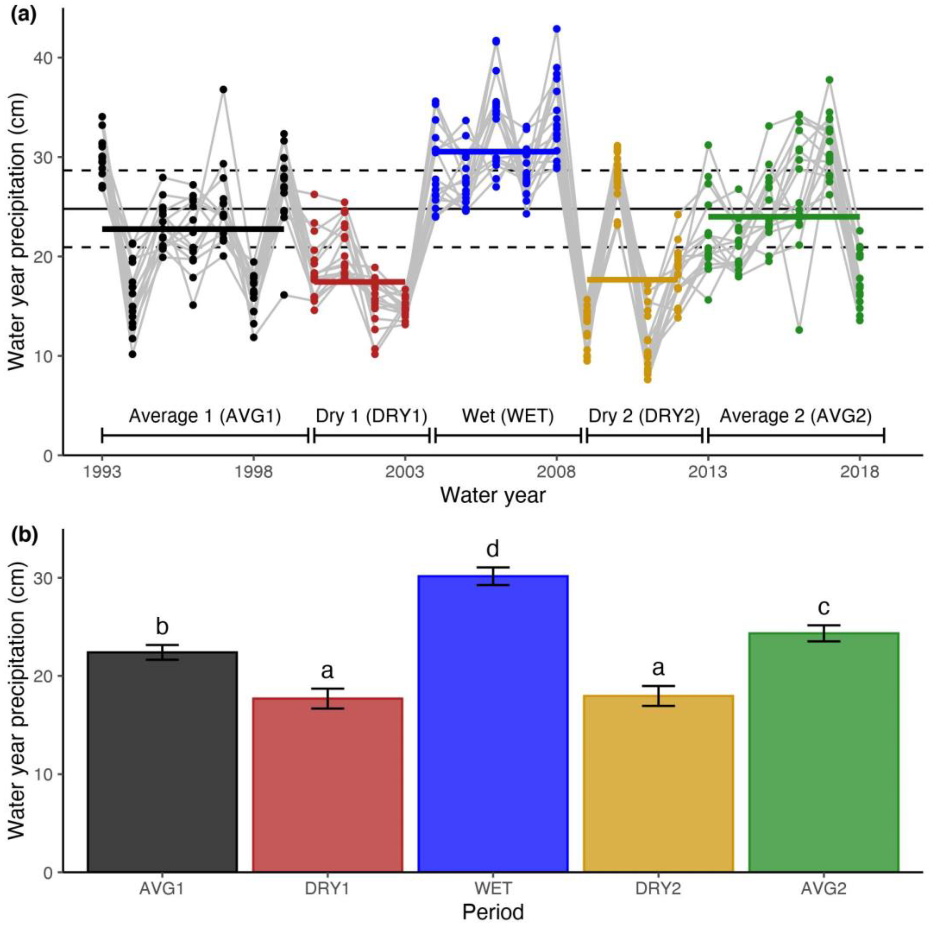
2.4.1. Objective 1: Identifying Precipitation Periods and Species Richness Responses

To define multiyear periods of similar precipitation, a breakpoint analysis was applied to the water-year precipitation data (WPPT; October 1 to September 30) averaged over the 16 precipitation locations in each year. Breakpoint analyses indicate when a statistically different year occurs during a time series [76,77]. These analyses have been used in ecological studies to identify thresholds in time series data that reflect important changes in ecosystem dynamics or the processes governing those dynamics [4,78]. The strucchange package in R was used to determine the optimal number of breakpoints and their locations in the mean water-year precipitation time series given a minimum window size and a quantitative measure to optimize [79,80]. For WPPT, we assumed a minimum window size of four years to account for legacy effects, and the number of years needed for sequential processes to occur (recruitment, growth, mortality) and result in population change in perennial grasses [16]. We optimized the residual sum of squares. We then compared mean WPPT among periods using a repeated measures ANOVA with subjects as the 16 locations and the fixed effect of period.
For the groups of species, log-transformed richness values for each group were analyzed to meet assumptions of normality, although nontransformed values are presented to aid in interpretation. Richness per functional group and ecosystem type were compared either between pairs of similar periods or among all five periods using a repeated measures ANOVA with the 12 locations as subjects and the fixed effect of period.

2.4.2. Objective 2: Comparing Daily Precipitation Characteristics and Richness for Periods with Similar Precipitation

We used characteristics of daily precipitation (storm depth, dry-day interval, frequency of dry and wet spells of different durations) to compare periods with similar amounts of mean precipitation across years within a period. Daily precipitation data were translated into two variables to interpret frequency distributions: storm depth (cm, daily rainfall amount >0.01 cm), and dry-day interval (number of sequential days between days with rain). Storm depth was based on precipitation amounts larger than a trace (>0.01 cm) for the rain gauges. Dry-day intervals were assigned to the season when the interval began, and were allowed to persist into later seasons. To characterize the distributions of the two variables, probability density functions (PDFs) were fit to their sample distributions using data from all 16 locations for each period and season. The exponential PDF was used because it is defined for non-negative numbers, has a general shape with greater probability density for small values with a decreasing right tail for lower probability density for high extreme values, has only one parameter to fit, and is typically used to describe daily PPT patterns [53,81], including across the western US [47].
For storm depth (h), an exponential PDF was fit to each period-season sample distribution:
f H ( h ) = 1 α e 1 α h
where 1/α is the parameter to estimate. Since the maximum likelihood estimator for the parameter in an exponential PDF is one divided by the sample mean of the random variable, α can be interpreted as mean storm depth (cm). Similarly, we fit an exponential PDF to the dry-day interval sample distributions:
f T ( t ) =   1 τ e 1 τ t
where τ can be interpreted as the mean dry-day interval (days). For each period and season, the storm depth and dry-day interval sample distributions were tested with Cramer-von Mises and Anderson-Darling goodness-of-fit tests (0.05 significance level) to assess the applicability of the exponential PDF for the samples. The α and τ parameters were estimated with bootstrapping (1001 iterations) to yield 95% confidence intervals. The fitdistrplus R package was used to fit the distributions with bootstrapping and to test goodness-of-fit [82]. For all periods and seasons, the storm depth and dry-day interval distributions had p-values greater than the significance threshold for both of the goodness-of-fit tests. Therefore, we can describe storm depth and dry-day interval distributions as exponential PDFs and compare the periods by their estimated mean storm depths (α) and mean dry-day intervals (τ).
We also calculated the number of days in each period in a dry spell (number of consecutive days with less rain than 0.5 cm/day) or wet spell (number of consecutive days with rain more than 0.5 cm/day) of varying duration. Dry or wet spell durations provide a more accurate depiction of the ecologically-relevant precipitation for plant growth than the dry-day interval, and are based on experimental responses in drylands [58,83]. Dry spell duration classes were selected to represent short (0, 1–3, 4–7 days), medium (8–14, 15–30 days), and long durations (31–100, 101–200, 201–365 days) for within-year dry periods. These classes correspond to plant physiological responses where short dry spells are less than a week, medium spells are 1 week to 1 month, and long dry spells are seasonal to annual. Within each season, dry spell frequency was calculated as the percentage of days classified as a dry spell. When a dry spell crossed into two or more seasons, it was counted in both seasons and weighted by the number of days it extended into each season. Similarly, wet spell duration (0, 1–9 days) was based on the length of sequential wet days. Each day was classified as a “wet spell” or “non-wet spell” based on whether it fit the definition. In each season, wet spell frequency was calculated as the percentage of days in a wet spell. A non-wet spell is the same as a dry spell except that a non-wet spell can be of any duration.

2.4.3. Objective 3: Comparing the Sequence of Wet-Dry Periods and Richness over the Record

To compare precipitation characteristics through time, we used metrics of seasonal and annual rainfall that captured extreme values. Total amount of precipitation (cm) was summed for each location within each season and averaged across all locations within each period. Precipitation frequency was defined as the percentage of days with precipitation exceeding a trace amount (0.01 cm/day). The frequency of extreme precipitation was defined as the percentage of days in each season with daily precipitation exceeding the 98th percentile of precipitation amount (0.7 cm/day in OND, 0.5 cm/day in JFM, 0.5 cm/day in AMJ, and 1.6 cm/day in JAS).
To compare the mean value of each precipitation metric among periods, a repeated measures ANOVA, with subjects as the 16 locations and period as a fixed effect, was applied to each metric and season pair individually. For each metric-season combination, the period effect was tested for significance and, if significant, the contrasts of each marginal mean pairs of periods were tested for significant differences. To assess changes in daily PPT amount and frequency through time, estimated mean storm depth and mean dry-day interval were compared between period pairs. If the 95% confidence intervals of the estimated parameters between two periods did not overlap, the parameters for those periods were considered significantly different.

3. Results

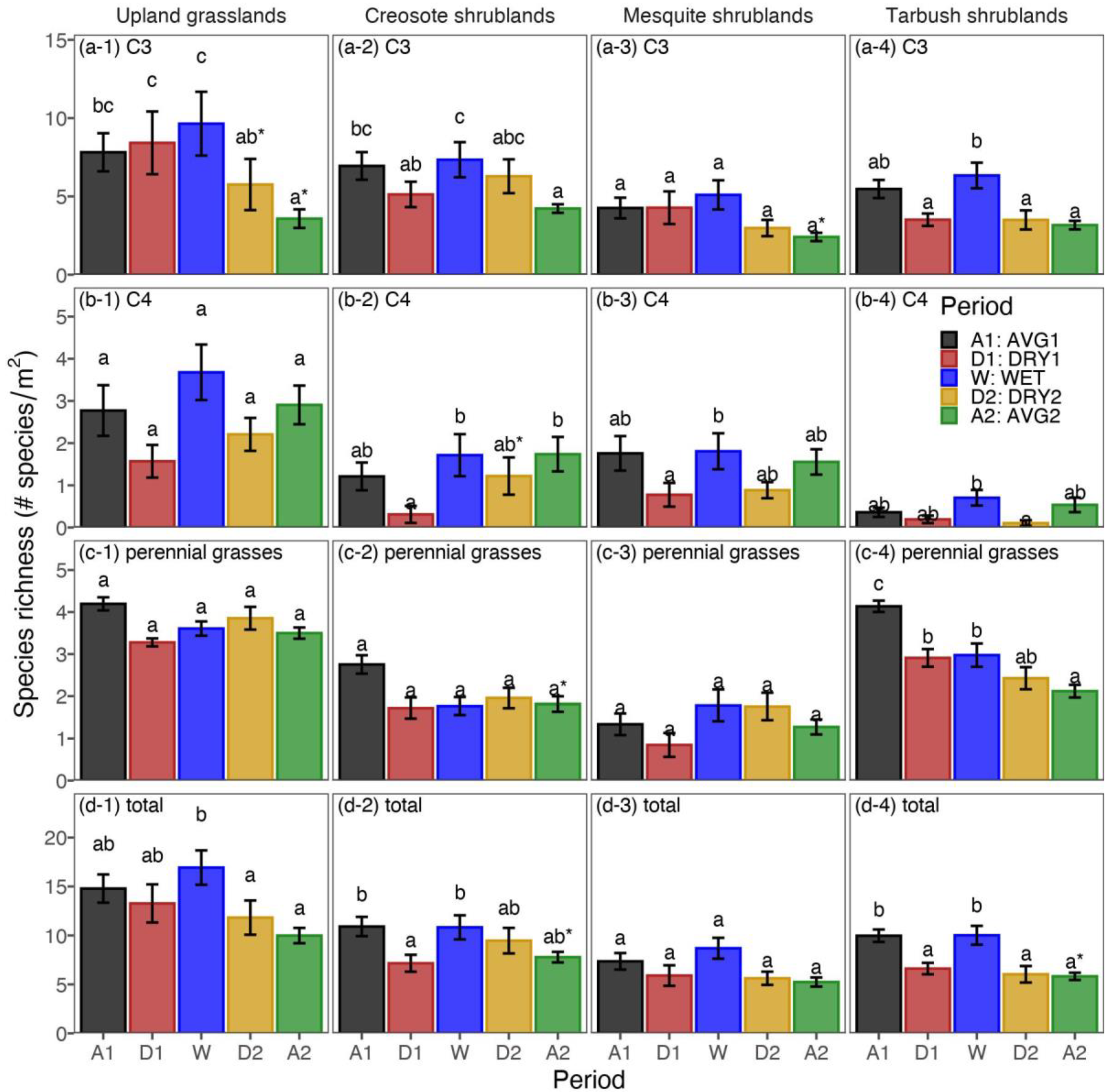
3.1. Objective 1: Identifying Precipitation Periods and Species Richness Responses

Using a window size of four years, the optimal number of breakpoints was four during the years 1999, 2003, 2008, and 2012. Five sequential periods were differentiated by their mean water-year precipitation: AVG1 (1993–1999), DRY1 (2000–2003), WET (2004–2008), DRY2 (2009–2012), and AVG2 (2013–2018) (Figure 1a). The WET period had the highest mean (30.2 cm/y) and the two DRY periods had similarly low mean precipitation (DRY1:17.7 cm/y; DRY2:18.0 cm/y) compared with the two average periods, where AVG1 (22.4 cm/y) had significantly less precipitation than AVG2 (24.3 cm/y) (Figure 1b). The first three periods agreed with previously defined periods using a qualitative approach for six of these locations [15].
In general, the largest numbers of species were found in upland grasslands followed by creosotebush, tarbush, and mesquite shrublands (Figure 2). Functional group composition was similar for all ecosystems: the C3 type (grasses, forbs, sub-shrubs, and shrubs) had the most species at all four ecosystems with perennial grasses second highest, and the C4 functional group had the fewest number of species.
Total species richness in the wet period was among the highest in the five periods (Figure 2. For other species-ecosystem combinations, two patterns were unrelated to total precipitation. AVG1 had more C3 species, yet lower water-year precipitation, compared with AVG2, in upland grasslands, creosote bush, and mesquite shrublands (Table 1, Figure 1b). While DRY1 and DRY2 had the same amount of precipitation, DRY2 had more C4 species than DRY1 in in creosote shrublands and DRY1 had more C3 species than DRY2 in upland grasslands (Table 1, Figure 1b).

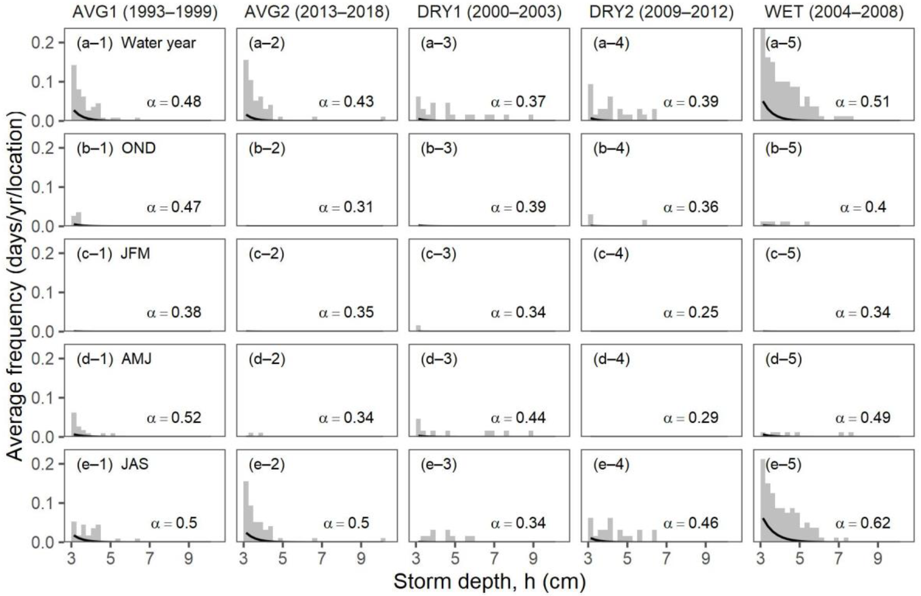
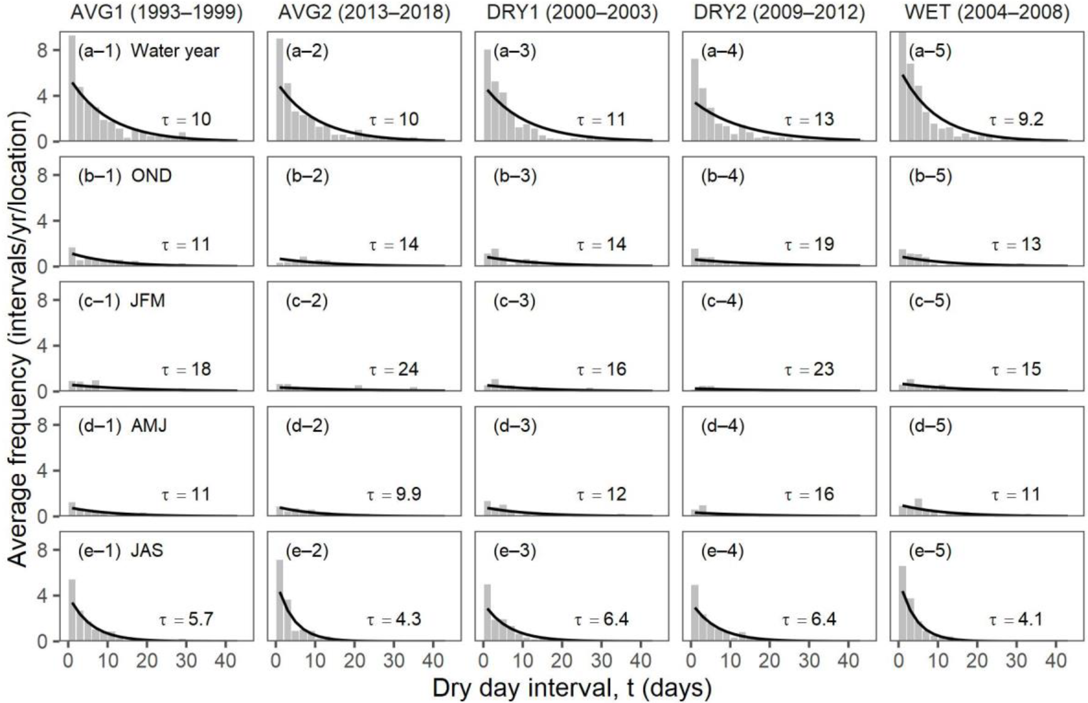
3.2. Objective 2: Comparing Daily Precipitation Characteristics and Richness for Periods with Similar Precipitation

The frequency distributions of storm depth sizes up to 3 cm showed a high proportion of small events in all seasons and periods with a sharp decrease in frequency as event size increased (Figure 3). Largest seasonal mean storm depth sizes occurred in the spring (AMJ) and summer (JAS) in AVG1 (α ≥ 0.5 cm), and in the summer in AVG2 (α = 0.5 cm), and WET (α = 0.62 cm). Storm depth sizes, on average, were smaller in the corresponding dry periods than in the average or wet periods in the same seasons (e.g., DRY1 vs. AVG 1 or WET in OND). Separating out small storm depth sizes (<3 cm) from large storm depth sizes (≥3 cm) allows a focus on the correspondence between large rain events and species richness (Table 1, Figure 2 and Figure 4). For example, more large storms in the fall (OND) and spring (AMJ) in AVG1 (Figure 4) corresponded with more C3 species at upland grasslands and creosotebush shrublands compared with AVG2 (Figure 2). DRY1 had more large storms than DRY2 in late spring (AMJ), and greater C3 species richness in upland grasslands. In contrast, DRY2 had more large storms than DRY1 in summer (JAS) and greater C4 species richness (other than perennial grasses) in creosotebush shrublands compared with fewer large storms and fewer C4 species in this ecosystem in DRY1 (Figure 2 and Figure 4).
The frequency distribution of the number of days between rain events (i.e., the dry-day interval) is skewed to the left, with most values < 10 days during the summer monsoon rainy season (JAS) when C4 species are most active (Figure 5). In the summer, the larger τ (5.7 days) in AVG1 reflects more dry-day intervals of longer lengths compared to AVG2 (τ = 4.3 days), and may correspond with the lower water year precipitation in AVG1 (Figure 1 and Figure 5). Flat curves in the other seasons indicate the few occurrences of long duration between rain events typical of drylands. The WET period had the fewest total long duration (>45 days between rain events) dry intervals of all periods in each season (Figure 6). The summer (JAS) had the fewest long dry intervals compared with the early spring (JFM) where AVG2 and DRY2 had more frequent, long dry intervals with greater τ values compared with AVG1 and DRY1, respectively. DRY2 had more long duration dry intervals in the fall (OND), and fewer C3 species richness (e.g., shrubs and sub-shrubs) in upland grasslands compared with DRY1 (Figure 2).
Differences in precipitation between periods were further distinguished by comparing storm depth (α) and dry-day interval (τ) parameters with patterns in species richness of functional groups. In fall (OND) and spring (AMJ), AVG1 had a larger mean storm depth and a smaller mean dry-day interval than AVG2 with more C3 species in AVG1 for all locations (Figure 2 and Figure 7a,c). Mean storm depths in spring (JFM) and summer (JAS) were not significantly different for these two periods. On the other hand, while the difference between dry-day intervals between AVG1 (τ = 5.7 days) and AVG2 (τ = 4.3 days) in summer (JAS) was small (Figure 7c), the AVG1 dry-day interval was 32% larger than AVG2.
In the dry periods, DRY2 had a greater mean storm depth and a 35% increase in precipitation when it rained (0.46 cm/day) over DRY1 on average (0.34 cm/day) in the summer (JAS) (Figure 4 and Figure 7b), and greater C4 richness in DRY2 for creosotebush shrublands (Figure 2). The greater storm depth and shorter dry-day intervals in DRY1 in the spring seasons (JFM, AMJ) compared with DRY2 corresponded with more C3 species in upland grasslands in DRY1 (Figure 2 and Figure 7b). In addition, DRY1 experienced more frequent rain days with more rain on those days in the spring (0.44 cm/day) compared with DRY2 (0.29 cm/day) (Figure 4).
The frequency of dry days of varying duration in different seasons is a measure of within- year dry spells (Figure 8). The frequency of short-duration (up to 7 days) dry spells during the summer growing season (JAS) was similar between DRY1 and DRY2, and between AVG1 and AVG2 (Figure 8d). However, DRY2 had more mid-duration dry spells in the summer (8–30 days) and greater richness of C4 species in creosotebush and mesquite-dominated shrublands than DRY1, whereas DRY1 had more long-duration dry spells (>30 days) (Figure 2 and Figure 8d). During spring (AMJ), DRY2 and AVG2 had more dry spells days lasting longer than 200 days and fewer C3 species in upland grasslands than DRY1 or AVG1, respectively (Figure 2 and Figure 8c).
The frequency of consecutive single day wet events (wet spells) showed seasonal variability between periods (Figure 9). In summer, there were more events with two or more consecutive wet days in DRY2 than in DRY1 that corresponded to C4 richness in creosotebush shrublands (Figure 9d). In addition, the frequency of one and two precipitation events in the summer, and the number of C4 species in creosote bush shrublands, were nearly identical between AVG2 and WET (Figure 2 and Figure 9d). AVG2 had the longest duration (9 day) wet spells with less total annual rainfall than WET (Figure 1). In the other seasons, the pattern was reversed from the summer: DRY1 and AVG1 had more frequent wet events than DRY2 and AVG2 that corresponded with C3 species richness in upland grasslands (Figure 2 and Figure 9).

3.3. Objective 3: Comparing the Sequence of Wet-Dry Periods and Richness over the Record

Fall (OND), winter (JFM) and spring (AMJ) precipitation amounts were similar among the first three periods (1993–2008) and then decreased through time. The result is that AVG2 had significantly less fall and spring precipitation than AVG1 (Figure 10). The delivery of that precipitation also changed: the frequency of precipitation in the 98th percentile (≥0.5 cm/day) decreased in fall and spring resulting in AVG1 and DRY1 having more extreme precipitation than AVG2 and DRY2 in these seasons (Figure 10).
The opposite trend was observed in the summer growing season (JAS), where precipitation amounts generally increased from beginning to end of the record (Figure 10) with a corresponding general increase in frequency of extreme rainfall events. The result is that DRY1 was substantially drier with less frequent precipitation than DRY2 in the summer, whereas the opposite was true in the other seasons. These rainfall patterns corresponded to C4 species richness in creosotebush shrublands (Figure 2). In addition, AVG2 had more frequent summer precipitation than AVG1 and even the WET period (Figure 10), and similar numbers of C4 annual species in all three shrubland types for AVG2 and the WET periods (Figure 2). The higher total precipitation in the summer in WET than AVG2 (Figure 10a) was associated with higher average precipitation totals on days with precipitation.
Comparing mean storm depth and mean dry-day interval for each period represents changes in mean seasonal precipitation through time [47]. For the growing season, each transition from one period to the next had significant differences in both storm depth and dry-day interval, although the direction of the change depended on the period preceding the period in question (Figure 11a). In both transitions to dry periods (i.e., AVG1 to DRY1; WET to DRY2), mean storm depth decreased and mean dry-day interval increased, while in both transitions from a dry period (i.e., DRY1 to WET; DRY2 to AVG2), meant storm depth increased and mean dry-day interval decreased. Thus, differences in growing season precipitation among all five periods can be attributed to both changes in daily precipitation amount (Figure 10a-4) and frequency (Figure 10c-4).
For the nongrowing season, a different pattern in time was observed where there was a decrease in mean storm depth from AVG1 to DRY1, then no significant difference from DRY1 to WET, then a decrease in mean storm depth and increase in mean dry-day interval from WET to DRY2, and then no significant difference from DRY2 to AVG2. This series of transition differences resulted in a general decrease in the amount of nongrowing season precipitation over the course of the study: first, daily precipitation amounts decreased, then daily precipitation frequency decreased. Several cases of losses of richness were observed: the number of perennial grasses in tarbush ecosystems decreased through time and decreased from AVG1 to AVG2 in creosotebush shrublands, and C3 species richness in all four ecosystem types decreased since the WET period (Figure 2).

4. Discussion

Distinguishing multiyear dry and wet periods from random sequences of years for a 26-year time series of precipitation data provided new insights into the relationships between rainfall and species richness compared to traditional studies of extreme events based on individual years [42]. Similar to expectations, the wet period with the largest mean amount of water-year precipitation had among the highest total species richness in the five periods for all four ecosystem types: upland grasslands, and the three shrubland types dominated by different species: creosotebush, mesquite, tarbush. We observed two patterns in species richness that required more in-depth analyses of daily and seasonal precipitation within each period to understand the potential processes underlying richness patterns. Compared with AVG2, AVG1 had lower water-year precipitation yet more C3 species in upland grasslands, creosotebush, and mesquite shrublands, and more C4 perennial grasses in tarbush shrublands. AVG1 had larger amounts of rainfall and more large storms in fall and spring with higher mean depths of storm and lower mean dry-day interval compared with AVG2. DRY1 and DRY2 had the same amount of precipitation, yet DRY2 had more C4 species than DRY1 in creosotebush shrublands and DRY1 had more C3 species than DRY2 in upland grasslands. Most differences in rainfall between these periods occurred in the summer when C4 species would be affected by soil water availability. Our results show that understanding the biodiversity of Chihuahuan Desert landscapes as precipitation continues to change will require daily and seasonal metrics of rainfall within a wet-dry period paradigm.

4.1. Richness and Rainfall Comparisons between Periods

Our results show that it is necessary to go beyond water-year amount of precipitation to understand the response of plant canopy species richness. Dry spell length was most frequently important to account for differences in richness between periods with similar water-year precipitation, followed by mean storm depth, total seasonal precipitation and extreme precipitation frequency (Table 1). Drylands are characterized by small rain event sizes and short duration between events that increase soil water availability to plants [46]. In our study, precipitation characteristics in the fall and spring were important for explaining richness of C3 species and perennial grasses primarily in average rainfall periods (AVG1, AVG2; Table 1, Figure 2 and Figure 10). Storm depth was also important where the size of individual storms affect the depth that water percolates into the soil [84]. The depth of the wetting front controls the partitioning of vertical water losses between soil evaporation, deep percolation, and transpiration. As predicted by the inverse texture hypothesis [25] and empirically demonstrated later [60,85,86], large rainfall events enhance soil water available to plants only in drylands.
Similar to previous studies, seasonality in these precipitation characteristics was also important to richness patterns (Table 1) [87]. These characteristics varied by period and ecosystem type that likely governed seasonal patterns in water availability [85,88]. The tendency for the WET period to have the greatest number of species for C3 and C4 functional groups across all ecosystem types was likely related to this period generally having the deepest average storm depth in the summer, and fewest long duration (>45 day) dry intervals across all seasons (Figure 3 and Figure 6). Both characteristics can affect water available to plants, either to C4 species including perennial grasses in the summer or to all species throughout the year [45].
The larger number of C3 species in upland grasslands and creosotebush species in AVG1, yet lower water-year precipitation, compared with AVG2, may be explained by larger amounts of rainfall and more large storms in AVG1 in fall and spring compared with AVG2 (Figure 10). The resulting precipitation had a higher mean storm depth and lower mean dry-day interval in AVG1 than AVG2, which would have resulted in more soil moisture during the seasons when C3 species are either actively growing (annuals, forbs, and grasses: AMJ) or can receive subsurface water recharge (shrubs and subshrubs: OND) [53,81,89]. By contrast, in summer, the AVG1 dry-day interval was 32% greater, and summer precipitation was lower than AVG2. However, none of our locations showed a species richness response in AVG2 to this shorter average dry-day interval and larger amount of summer rainfall compared with AVG1 (Figure 2 and Figure 10). This result suggests that other factors are driving richness in the summer for these locations on the dryland landscapes, such as competition with the dominant C4 perennial grasses or a legacy effect of the WET or preceding dry period (DRY2).
Differences in seasonality of rainfall between periods with similar amounts of total rainfall may reflect changing rainfall patterns through time. Both AVG1 and DRY1 have higher fall and lower summer amounts of rainfall than AVG2 and DRY2, respectively. A shift from less fall to more summer rainfall could explain the general loss in C3 species at most locations through time. Reclassifying periods to account for both patterns in precipitation and vegetation may be warranted with further research.
Interestingly, the opposite pattern was found for the dry periods (DRY1, DRY2) and C4 species richness in creosotebush shrublands. The number of events, event size, and length of dry periods of similar rainfall amounts have been shown to be important to grassland production in drylands [17]. In our study, more C4 species occurred in DRY2 than DRY1 even though both periods had similar amounts of water-year precipitation (Table 1). Most differences between these periods occurred in the summer, when C4 species would be affected by soil water availability. Both dry periods had long, dry intervals (>30 days) during the summer (JAS), although DRY1 had a greater frequency of dry-day intervals from 31 to 200 days that would have resulted in less soil moisture compared to DRY2 [89]. In addition, DRY1 was substantially drier, with less frequent precipitation than DRY2, which had more frequent large storms in the summer (Table 1). There were also more events with two or more consecutive wet days in DRY2 (Figure 9, Table 1).

4.2. Importance of Legacies

Our time series of richness and precipitation data allow us to compare the legacy of a dry period (DRY1) in a subsequent wet period (WET) with the legacy of a very wet period (WET) in a subsequent dry period (DRY2). As expected, based on theory and precipitation manipulation experiments, these two legacies were asymmetrical [26,27]. The legacy of a wet period had a larger negative effect on richness compared with the legacy of a dry period. This legacy effect was important for C3 species richness in upland grasslands where the transition from DRY1 (8.4 species/m2) to WET (9.6 species/m2) led to no significant change in richness compared with the transition from WET to DRY2 (5.7 species/m2), which resulted in a 41% loss of C3 annual and perennial subdominant species (Figure 2). Based on previous research, we expect the mechanisms of the two legacy periods were different. A dry period (DRY1) with few meristems and low seed production may have dampened the C3 species responses in the WET period, whereas the lower richness than expected in DRY2 may have resulted from the larger densities of C4 dominant perennials in the WET period that survived through time [27,56].
The opposite asymmetry pattern was found for C4 subdominant species in creosote bush and mesquite shrublands, where an increase in richness occurred from DRY1 to WET followed by no change in richness from WET to DRY2. These results show that C4 subdominant species can respond in shrublands to a sequence of years of above-average years of precipitation and can then persist through time during a subsequent multiyear drought. In creosote bush, the effect of the wet period continued to persist into the second average period (AVG2) with similar richness values as the WET period, yet with significantly less rainfall (Figure 1 and Figure 2). Islands of fertility associated with creosotebush shrubs combined with modifications of soil properties from herbaceous plants during the WET period may have accounted for the continued success of these C4 plants.

5. Conclusions

This study highlighted the importance of studying multiyear precipitation patterns as important drivers of ecosystem structure. Patterns in precipitation have shifted at this research site over the past 26 years, during which nongrowing precipitation amount has decreased and the summer growing season has increased with a corresponding increase in frequency of extreme rainfall events. Water-year amount was not sufficient to explain long-term patterns in plant-species richness. These empirical observations confirmed results from experiments performed with an ecosystem level model [90]. The modelling exercise explored the importance of enhancing the amount of annual precipitation variability by enhancing or decreasing subsequent event sizes by 25, 50 or 75% versus enhancing the duration of a dry period or extreme wet conditions from 1, 3, 6 and 9 years. The model showed that duration of dry and wet periods had the largest effect on ecosystem water balance by affecting the soil wetting depth. Modelling, and this study, support the importance of storm depth on ecosystem structure (species richness) and functioning (soil water dynamics). Moreover, penetration of water in the soil profile is affected by the duration of the wet or dry conditions. Our results confirm the theory that niche partitioning and, consequently, species richness in drylands are determined by the distribution of belowground resources and traits associated with species physiology and rooting patterns [91]. In addition, our study of multiple periods with similar amounts of water-year rainfall, yet different ecosystem responses, show the importance of considering the biotic and precipitation characteristics of multiple multiyear periods rather than inferring generalizations from individual extreme events. Long-term observations will be needed to characterize and develop these generalizations from multiple multiyear periods.

Author Contributions

Conceptualization and methodology, D.P.C.P., O.E.S., E.R.V.; formal analysis, H.M.S., S.S., H.H., A.R.H.; writing–original draft preparation, D.P.C.P., H.M.S., S.S., H.H.; writing–review and editing, all authors; visualization, H.M.S., S.S., H.H.; supervision, D.P.C.P.; funding acquisition, D.P.C.P. All authors have read and agreed to the published version of the manuscript.

Funding

This research was funded by the National Science Foundation to New Mexico State University for the Jornada Basin Long Term Ecological Research Program (DEB 20-2025166), the USDA-ARS CRIS Project at the Jornada Experimental Range (#6235-11210-007), and the USDA-ARS SCINet Big Data Project ARS project number 0500-00093-001-00-D.

Data Availability Statement

Data available from the Environmental Data Initiative include the gap-filled daily precipitation from the NPP study locations (knb-lter-jrn.210425001.75), daily and approximately weekly precipitation data from the LTER weather station (knb-lter-jrn.210126001.113; knb-lter-jrn.210126003.100), and species richness data from the NPP study (knb-lter-jrn.210011002.106). Citations for the data packages are given as they appear in the text.

Acknowledgments

We thank Laura Huenneke for initiating the long-term NPP study that collects the species richness data, and John Anderson and the LTER field technicians for collecting the species richness data through time. We thank Gregory S. Okin and Brandon T. Bestelmeyer for discussions during the development of this study.

Conflicts of Interest

The authors declare no conflict of interest.

References

  1. Donat, M.G.; Lowry, A.L.; Alexander, L.V.; O’Gorman, P.A.; Maher, N. More Extreme Precipitation in the World’s Dry and Wet Regions. Nat. Clim. Chang. 2016, 6, 508–513. [Google Scholar] [CrossRef]
  2. Pendergrass, A.G.; Knutti, R.; Lehner, F.; Deser, C.; Sanderson, B.M. Precipitation Variability Increases in a Warmer Climate. Sci. Rep. 2017, 7, 17966. [Google Scholar] [CrossRef] [PubMed] [Green Version]
  3. Alvarez, L.J.; Epstein, H.E.; Li, J.; Okin, G.S. Aeolian Process Effects on Vegetation Communities in an Arid Grassland Ecosystem. Ecol. Evol. 2012, 2, 809–821. [Google Scholar] [CrossRef] [PubMed]
  4. Bestelmeyer, B.T.; Ellison, A.M.; Fraser, W.R.; Gorman, K.B.; Holbrook, S.J.; Laney, C.M.; Ohman, M.D.; Peters, D.P.C.; Pillsbury, F.C.; Rassweiler, A.; et al. Analysis of Abrupt Transitions in Ecological Systems. Ecosphere 2011, 2, 129. [Google Scholar] [CrossRef]
  5. Hoover, D.L.; Knapp, A.K.; Smith, M.D. Resistance and Resilience of a Grassland Ecosystem to Climate Extremes. Ecology 2014, 95, 2646–2656. [Google Scholar] [CrossRef] [Green Version]
  6. Okin, G.S.; Sala, O.E.; Vivoni, E.R.; Zhang, J.; Bhattachan, A. The Interactive Role of Wind and Water in Functioning of Drylands: What Does the Future Hold? Bioscience 2018, 68, 670–677. [Google Scholar] [CrossRef]
  7. Peters, D.P.C.; Bestelmeyer, B.T.; Herrick, J.E.; Fredrickson, E.L.; Monger, H.C.; Havstad, K.M. Disentangling Complex Landscapes: New Insights into Arid and Semiarid System Dynamics. Bioscience 2006, 56, 491–501. [Google Scholar] [CrossRef] [Green Version]
  8. Petrie, M.D.; Peters, D.P.C.; Yao, J.; Blair, J.M.; Burruss, N.D.; Collins, S.L.; Derner, J.D.; Gherardi, L.A.; Hendrickson, J.R.; Sala, O.E.; et al. Regional Grassland Productivity Responses to Precipitation during Multiyear Above- and below-Average Rainfall Periods. Glob. Chang. Biol. 2018, 24, 1935–1951. [Google Scholar] [CrossRef]
  9. Petrie, M.D.; Peters, D.P.C.; Burruss, N.D.; Ji, W.; Savoy, H.M. Differing Climate and Landscape Effects on Regional Dryland Vegetation Responses during Wet Periods Allude to Future Patterns. Glob. Chang. Biol. 2019, 25, 3305–3318. [Google Scholar] [CrossRef]
  10. Petrie, M.D.; Peters, D.P.C.; Burruss, N.D.; Ji, W.; Savoy, H.M. Local-regional similarity in drylands increases during multiyear wet and dry periods and in response to extreme events. Ecosphere 2019, 10, e02939. [Google Scholar] [CrossRef] [Green Version]
  11. Schreiner-McGraw, A.; Ajami, H.; Vivoni, E.R. Extreme Weather Events and Transmission Losses in Arid Streams. Environ. Res. Lett. 2019, 14, 084002. [Google Scholar] [CrossRef]
  12. Smith, M.D. An Ecological Perspective on Extreme Climatic Events: A Synthetic Definition and Framework to Guide Future Research. J. Ecol. 2011, 99, 656–663. [Google Scholar] [CrossRef]
  13. Estiarte, M.; Vicca, S.; Peñuelas, J.; Bahn, M.; Beier, C.; Emmett, B.A.; Fay, P.A.; Hanson, P.J.; Hasibeder, R.; Kigel, J.; et al. Few Multiyear Precipitation-Reduction Experiments Find a Shift in the Productivity-Precipitation Relationship. Glob. Chang. Biol. 2016, 22, 2570–2581. [Google Scholar] [CrossRef] [Green Version]
  14. Knapp, A.K.; Chen, A.; Griffin-Nolan, R.J.; Baur, L.E.; Carroll, C.J.W.; Gray, J.E.; Hoffman, A.M.; Li, X.; Post, A.K.; Slette, I.J.; et al. Resolving the Dust Bowl Paradox of Grassland Responses to Extreme Drought. Proc. Natl. Acad. Sci. USA 2020, 117, 22249–22255. [Google Scholar] [CrossRef]
  15. Peters, D.P.C.; Yao, J.; Sala, O.E.; Anderson, J.P. Directional Climate Change and Potential Reversal of Desertification in Arid and Semiarid Ecosystems. Glob. Chang. Biol. 2012, 18, 151–163. [Google Scholar] [CrossRef] [Green Version]
  16. Peters, D.P.C.; Yao, J.; Browning, D.; Rango, A. Mechanisms of Grass Response in Grasslands and Shrublands during Dry or Wet Periods. Oecologia 2014, 174, 1323–1334. [Google Scholar] [CrossRef]
  17. Carroll, C.J.W.; Slette, I.J.; Griffin-Nolan, R.J.; Baur, L.E.; Hoffman, A.M.; Denton, E.M.; Gray, J.E.; Post, A.K.; Johnston, M.K.; Yu, Q.; et al. Is a Drought a Drought in Grasslands? Productivity Responses to Different Types of Drought. Oecologia 2021, 1–10. [Google Scholar] [CrossRef]
  18. Collins, S.L.; Koerner, S.E.; Plaut, J.A.; Okie, J.G.; Brese, D.; Calabrese, L.B.; Carvajal, A.; Evansen, R.J.; Nonaka, E. Stability of Tallgrass Prairie during a 19-Year Increase in Growing Season Precipitation. Funct. Ecol. 2012, 26, 1450–1459. [Google Scholar] [CrossRef]
  19. Peters, D.P.C.; Burruss, N.D.; Okin, G.S.; Hatfield, J.L.; Scroggs, S.L.P.; Huang, H.; Brungard, C.W.; Yao, J. Deciphering the Past to Inform the Future: Preparing for the next (“Really Big”) Extreme Event. Front. Ecol. Environ. 2020, 18, 401–408. [Google Scholar] [CrossRef] [Green Version]
  20. Albertson, F.W.; Weaver, J.E. History of the Native Vegetation of Western Kansas during Seven Years of Continuous Drought. Ecol. Monogr. 1942, 12, 23–51. [Google Scholar] [CrossRef] [Green Version]
  21. Knapp, A.K.; Beier, C.; Briske, D.D.; Classen, A.T.; Luo, Y.; Reichstein, M.; Smith, M.D.; Smith, S.D.; Bell, J.E.; Fay, P.A.; et al. Consequences of More Extreme Precipitation Regimes for Terrestrial Ecosystems. Bioscience 2008, 58, 811–821. [Google Scholar] [CrossRef]
  22. Seneviratne, S.I.; Nicholls, N.; Easterling, D.; Goodess, C.M.; Kanae, S.; Kossin, J.; Luo, Y.; Marengo, J.; McInnes, K.; Rahimi, M.; et al. Changes in Climate Extremes and their Impacts on the Natural Physical Environment. In Managing the Risks of Extreme Events and Disasters to Advance Climate Change Adaptation; Field, C.B., Barros, V., Stocker, T.F., Dahe, Q., Eds.; Cambridge University Press: Cambridge, UK, 2012; pp. 109–230. ISBN 9781139177245. [Google Scholar]
  23. Schwinning, S.; Sala, O.E. Hierarchy of Responses to Resource Pulses in Arid and Semi-Arid Ecosystems. Oecologia 2004, 141, 211–220. [Google Scholar] [CrossRef]
  24. Reynolds, J.F.; Kemp, P.R.; Ogle, K.; Fernández, R.J. Modifying the ‘Pulse–Reserve’ Paradigm for Deserts of North America: Precipitation Pulses, Soil Water, and Plant Responses. Oecologia 2004, 141, 194–210. [Google Scholar] [CrossRef]
  25. Noy-Meir, I. Desert Ecosystems: Environment and Producers. Annu. Rev. Ecol. Syst. 1973, 4, 25–52. [Google Scholar] [CrossRef]
  26. Sala, O.E.; Gherardi, L.A.; Reichmann, L.; Jobbágy, E.; Peters, D. Legacies of Precipitation Fluctuations on Primary Production: Theory and Data Synthesis. Philos. Trans. R. Soc. B Biol. Sci. 2012, 367, 3135–3144. [Google Scholar] [CrossRef] [PubMed] [Green Version]
  27. Reichmann, L.G.; Sala, O.E.; Peters, D.P.C. Precipitation Legacies in Desert Grassland Primary Production Occur through Previous-Year Tiller Density. Ecology 2013, 94, 435–443. [Google Scholar] [CrossRef] [PubMed]
  28. Knapp, A.K. Rainfall Variability, Carbon Cycling, and Plant Species Diversity in a Mesic Grassland. Science 2002, 298, 2202–2205. [Google Scholar] [CrossRef] [PubMed] [Green Version]
  29. Maestre, F.T.; Quero, J.L.; Gotelli, N.J.; Escudero, A.; Ochoa, V.; Delgado-Baquerizo, M.; Garcia-Gomez, M.; Bowker, M.A.; Soliveres, S.; Escolar, C.; et al. Plant Species Richness and Ecosystem Multifunctionality in Global Drylands. Science 2012, 335, 214–218. [Google Scholar] [CrossRef] [PubMed] [Green Version]
  30. Hector, A.; Hautier, Y.; Saner, P.; Wacker, L.; Bagchi, R.; Joshi, J.; Scherer-Lorenzen, M.; Spehn, E.M.; Bazeley-White, E.; Weilenmann, M.; et al. General Stabilizing Effects of Plant Diversity on Grassland Productivity through Population Asynchrony and Overyielding. Ecology 2010, 91, 2213–2220. [Google Scholar] [CrossRef] [PubMed]
  31. Isbell, F.; Craven, D.; Connolly, J.; Loreau, M.; Schmid, B.; Beierkuhnlein, C.; Bezemer, T.M.; Bonin, C.; Bruelheide, H.; de Luca, E.; et al. Biodiversity Increases the Resistance of Ecosystem Productivity to Climate Extremes. Nature 2015, 526, 574–577. [Google Scholar] [CrossRef] [PubMed]
  32. Tilman, D.; Downing, J.A. Biodiversity and Stability in Grasslands. Nature 1994, 367, 363–365. [Google Scholar] [CrossRef]
  33. Tilman, D.; Reich, P.B.; Knops, J.M.H. Biodiversity and Ecosystem Stability in a Decade-Long Grassland Experiment. Nature 2006, 441, 629–632. [Google Scholar] [CrossRef]
  34. Hector, A.; Schmid, B.; Beierkuhnlein, C.; Caldeira, M.C.; Diemer, M.; Dimitrakopoulos, P.G.; Finn, J.A.; Freitas, H.; Giller, P.S.; Good, J.; et al. Plant Diversity and Productivity Experiments in European Grasslands. Science 1999, 286, 1123–1127. [Google Scholar] [CrossRef] [PubMed] [Green Version]
  35. Gross, K.; Cardinale, B.J.; Fox, J.W.; Gonzalez, A.; Loreau, M.; Wayne Polley, H.; Reich, P.B.; van Ruijven, J. Species Richness and the Temporal Stability of Biomass Production: A New Analysis of Recent Biodiversity Experiments. Am. Nat. 2014, 183, 1–12. [Google Scholar] [CrossRef] [Green Version]
  36. Hautier, Y.; Seabloom, E.W.; Borer, E.T.; Adler, P.B.; Harpole, W.S.; Hillebrand, H.; Lind, E.M.; MacDougall, A.S.; Stevens, C.J.; Bakker, J.D.; et al. Eutrophication Weakens Stabilizing Effects of Diversity in Natural Grasslands. Nature 2014, 508, 521–525. [Google Scholar] [CrossRef]
  37. Hautier, Y.; Tilman, D.; Isbell, F.; Seabloom, E.W.; Borer, E.T.; Reich, P.B. Anthropogenic Environmental Changes Affect Ecosystem Stability via Biodiversity. Science 2015, 348, 336–340. [Google Scholar] [CrossRef] [Green Version]
  38. Gherardi, L.A.; Sala, O.E. Enhanced Interannual Precipitation Variability Increases Plant Functional Diversity That in Turn Ameliorates Negative Impact on Productivity. Ecol. Lett. 2015, 18, 1293–1300. [Google Scholar] [CrossRef]
  39. Griffin-Nolan, R.J.; Carroll, C.J.W.; Denton, E.M.; Johnston, M.K.; Collins, S.L.; Smith, M.D.; Knapp, A.K. Legacy Effects of a Regional Drought on Aboveground Net Primary Production in Six Central US Grasslands. Plant Ecol. 2018, 219, 505–515. [Google Scholar] [CrossRef]
  40. Frenette-Dussault, C.; Shipley, B.; Léger, J.-F.; Meziane, D.; Hingrat, Y. Functional Structure of an Arid Steppe Plant Community Reveals Similarities with Grime’s C-S-R Theory. J. Veg. Sci. 2012, 23, 208–222. [Google Scholar] [CrossRef]
  41. Kooyers, N.J. The Evolution of Drought Escape and Avoidance in Natural Herbaceous Populations. Plant Sci. 2015, 234, 155–162. [Google Scholar] [CrossRef]
  42. Arnone, J.A.; Jasoni, R.L.; Lucchesi, A.J.; Larsen, J.D.; Leger, E.A.; Sherry, R.A.; Luo, Y.; Schimel, D.S.; Verburg, P.S.J. A Climatically Extreme Year Has Large Impacts on C4 Species in Tallgrass Prairie Ecosystems but Only Minor Effects on Species Richness and Other Plant Functional Groups. J. Ecol. 2011, 99, 678–688. [Google Scholar] [CrossRef]
  43. Gherardi, L.A.; Sala, O.E. Enhanced Precipitation Variability Decreases Grass- and Increases Shrub-Productivity. Proc. Natl. Acad. Sci. USA 2015, 112, 12735–12740. [Google Scholar] [CrossRef] [Green Version]
  44. Suttle, K.B.; Thomsen, M.A.; Power, M.E. Species Interactions Reverse Grassland Responses to Changing Climate. Science 2007, 315, 640–642. [Google Scholar] [CrossRef] [Green Version]
  45. Duniway, M.C.; Petrie, M.D.; Peters, D.P.C.; Anderson, J.P.; Crossland, K.; Herrick, J.E. Soil Water Dynamics at 15 Locations Distributed across a Desert Landscape: Insights from a 27-Yr Dataset. Ecosphere 2018, 9, e02335. [Google Scholar] [CrossRef] [Green Version]
  46. Loik, M.E.; Breshears, D.D.; Lauenroth, W.K.; Belnap, J. A Multi-Scale Perspective of Water Pulses in Dryland Ecosystems: Climatology and Ecohydrology of the Western USA. Oecologia 2004, 141, 269–281. [Google Scholar] [CrossRef]
  47. Small, E.E. Climatic Controls on Diffuse Groundwater Recharge in Semiarid Environments of the Southwestern United States. Water Resour. Res. 2005, 41, 1–17. [Google Scholar] [CrossRef]
  48. Grant, K.; Kreyling, J.; Dienstbach, L.F.H.; Beierkuhnlein, C.; Jentsch, A. Water Stress Due to Increased Intra-Annual Precipitation Variability Reduced Forage Yield but Raised Forage Quality of a Temperate Grassland. Agric. Ecosyst. Environ. 2014, 186, 11–22. [Google Scholar] [CrossRef]
  49. Grant, K.; Kreyling, J.; Beierkuhnlein, C.; Jentsch, A. Importance of Seasonality for the Response of a Mesic Temperate Grassland to Increased Precipitation Variability and Warming. Ecosystems 2017, 20, 1454–1467. [Google Scholar] [CrossRef]
  50. Gibbens, R.P.; Lenz, J.M. Root Systems of Some Chihuahuan Desert Plants. J. Arid Environ. 2001, 49, 221–263. [Google Scholar] [CrossRef]
  51. Kurc, S.A.; Small, E.E. Dynamics of Evapotranspiration in Semiarid Grassland and Shrubland Ecosystems during the Summer Monsoon Season, Central New Mexico. Water Resour. Res. 2004, 40. [Google Scholar] [CrossRef]
  52. Felton, A.J.; Slette, I.J.; Smith, M.D.; Knapp, A.K. Precipitation Amount and Event Size Interact to Reduce Ecosystem Functioning during Dry Years in a Mesic Grassland. Glob. Chang. Biol. 2020, 26, 658–668. [Google Scholar] [CrossRef]
  53. Porporato, A.; Laio, F.; Ridolfi, L.; Caylor, K.K.; Rodriguez-Iturbe, I. Soil Moisture and Plant Stress Dynamics along the Kalahari Precipitation Gradient. J. Geophys. Res. Atmos. 2003, 108, 1–8. [Google Scholar] [CrossRef]
  54. Rodriguez-Iturbe, I.; Porporato, A.; Laio, F.; Ridolfi, L. Plants in Water-Controlled Ecosystems: Active Role in Hydrologic Processes and Response to Water Stress. Adv. Water Resour. 2001, 24, 695–705. [Google Scholar] [CrossRef]
  55. Fernandez-Illescas, C.P.; Porporato, A.; Laio, F.; Rodriguez-Iturbe, I. The Ecohydrological Role of Soil Texture in a Water-Limited Ecosystem. Water Resour. Res. 2001, 37, 2863–2872. [Google Scholar] [CrossRef]
  56. Monger, C.; Sala, O.E.; Duniway, M.C.; Goldfus, H.; Meir, I.A.; Poch, R.M.; Throop, H.L.; Vivoni, E.R. Legacy Effects in Linked Ecological–Soil–Geomorphic Systems of Drylands. Front. Ecol. Environ. 2015, 13, 13–19. [Google Scholar] [CrossRef] [Green Version]
  57. Reichmann, L.G.; Sala, O.E. Differential Sensitivities of Grassland Structural Components to Changes in Precipitation Mediate Productivity Response in a Desert Ecosystem. Funct. Ecol. 2014, 28, 1292–1298. [Google Scholar] [CrossRef] [Green Version]
  58. Thomey, M.L.; Collins, S.L.; Vargas, R.; Johnson, J.E.; Brown, R.F.; Natvig, D.O.; Friggens, M.T. Effect of Precipitation Variability on Net Primary Production and Soil Respiration in a Chihuahuan Desert Grassland. Glob. Chang. Biol. 2011, 17, 1505–1515. [Google Scholar] [CrossRef]
  59. Gherardi, L.A.; Sala, O.E. Effect of Interannual Precipitation Variability on Dryland Productivity: A Global Synthesis. Glob. Chang. Biol. 2019, 25, 269–276. [Google Scholar] [CrossRef] [Green Version]
  60. Heisler-White, J.L.; Blairr, J.M.; Kelly, E.F.; Harmoney, K.; Knapp, A.K. Contingent Productivity Responses to More Extreme Rainfall Regimes across a Grassland Biome. Glob. Chang. Biol. 2009, 15, 2894–2904. [Google Scholar] [CrossRef]
  61. IPCC. Global Warming of 1.5 °C. An IPCC Special Report on the Impacts of Global Warming of 1.5 °C above Pre-Industrial Levels and Related Global Greenhouse Gas Emission Pathways, in the Context of Strengthening the Global Response to the Threat of Climate Change; Masson-Delmotte, V., Zhai, P., Pörtner, H.-O., Roberts, D., Skea, J., Shukla, P.R., Pirani, A., Eds.; World Meteorological Organization: Geneva, Switzerland, 2018. [Google Scholar]
  62. Gibbens, R.P.; McNeely, R.P.; Havstad, K.M.; Beck, R.F.; Nolen, B. Vegetation Changes in the Jornada Basin from 1858 to 1998. J. Arid Environ. 2005, 61, 651–668. [Google Scholar] [CrossRef]
  63. Huenneke, L.F.; Anderson, J.P.; Remmenga, M.; Schlesinger, W.H. Desertification Alters Patterns of Aboveground Net Primary Production in Chihuahuan Ecosystems. Glob. Chang. Biol. 2002, 8, 247–264. [Google Scholar] [CrossRef]
  64. Li, J.; Okin, G.S.; Alvarez, L.; Epstein, H. Effects of Wind Erosion on the Spatial Heterogeneity of Soil Nutrients in Two Desert Grassland Communities. Biogeochemistry 2008, 88, 73–88. [Google Scholar] [CrossRef]
  65. Schlesinger, W.H.; Reynolds, J.F.; Cunningham, G.L.; Huenneke, L.F.; Jarrell, W.M.; Virginia, R.A.; Whitford, W.G. Biological Feedbacks in Global Desertification. Science 1990, 247, 1043–1048. [Google Scholar] [CrossRef] [Green Version]
  66. Pierce, N.A.; Archer, S.R.; Bestelmeyer, B.T.; James, D.K. Grass-Shrub Competition in Arid Lands: An Overlooked Driver in Grassland–Shrubland State Transition? Ecosystems 2019, 22, 619–628. [Google Scholar] [CrossRef]
  67. Manning, S.J.; Barbour, M.G. Root Systems, Spatial Patterns, and Competition for Soil Moisture between Two Desert Subshrubs. Am. J. Bot. 1988, 75, 885–893. [Google Scholar] [CrossRef]
  68. Fredrickson, E.; Havstad, K.M.; Estell, R.; Hyder, P. Perspectives on Desertification: South-Western United States. J. Arid Environ. 1998, 39, 191–207. [Google Scholar] [CrossRef]
  69. Anderson, J.P. LTER Weather Station Daily Summary Climate Data Ver 113. Available online: https://0-doi-org.brum.beds.ac.uk/10.6073/pasta/c13106744e57bae0f626bba25b635e0a (accessed on 12 August 2020).
  70. Anderson, J.P. Precipitation Data from a Standard Can Rain Gauge at the LTER Weather Station, Jornada Basin, Southern New Mexico, USA, 1992-Ongoing Ver 100. Available online: https://0-doi-org.brum.beds.ac.uk/10.6073/pasta/559d8d1fa1c542b8ad8088b65b48081b (accessed on 12 August 2020).
  71. Yao, J.; Anderson, J.P.; Savoy, H.; Peters, D.P.C. Gap-Filled Daily Precipitation at the 15 Long-Term NPP Sites at Jornada Basin LTER, 1980-Ongoing Ver 75. Available online: https://0-doi-org.brum.beds.ac.uk/10.6073/pasta/cf3c45e5480551453f1f9041d664a28f (accessed on 12 August 2020).
  72. Huenneke, L.F.; Clason, D.; Muldavin, E. Spatial Heterogeneity in Chihuahuan Desert Vegetation: Implications for Sampling Methods in Semi-Arid Ecosystems. J. Arid Environ. 2001, 47, 257–270. [Google Scholar] [CrossRef]
  73. Peters, D.P.C.; Huenneke., L.F. Seasonal Non-Destructive Vegetation Measurements at 15 Net Primary Production (NPP) Study Sites at Jornada Basin LTER, 1989-Ongoing Ver 106. Available online: https://0-doi-org.brum.beds.ac.uk/10.6073/pasta/18dad6748af96c98b72cea3436bf7fe4 (accessed on 16 December 2020).
  74. Pinheiro, J.; Bates, D.; DebRoy, S.; Sarkar, D.; Team, R.C. Linear and nonlinear mixed effects models. R Package Version 2019, 3, 1–89. [Google Scholar]
  75. Lenth, R. Emmeans: Estimated marginal means, aka least-squares means. R Package Version 1.4 2018, 1, 3. [Google Scholar]
  76. Saros, J.E.; Anderson, N.J.; Juggins, S.; McGowan, S.; Yde, J.C.; Telling, J.; Bullard, J.E.; Yallop, M.L.; Heathcote, A.J.; Burpee, B.T.; et al. Arctic Climate Shifts Drive Rapid Ecosystem Responses across the West Greenland Landscape. Environ. Res. Lett. 2019, 14, 074027. [Google Scholar] [CrossRef]
  77. Xu, L.; Yu, G.; Zhang, W.; Tu, Z.; Tan, W. Change Features of Time-Series Climate Variables from 1962 to 2016 in Inner Mongolia, China. J. Arid Land 2020, 12, 58–72. [Google Scholar] [CrossRef] [Green Version]
  78. Browning, D.M.; Maynard, J.J.; Karl, J.W.; Peters, D.C. Breaks in MODIS Time Series Portend Vegetation Change: Verification Using Long-Term Data in an Arid Grassland Ecosystem. Ecol. Appl. 2017, 27, 1677–1693. [Google Scholar] [CrossRef]
  79. Zeileis, A.; Leisch, F.; Hornik, K.; Kleiber, C. Strucchange: An R Package for Testing for Structural Change in Linear Regression Models. J. Stat. Softw. 2002, 7, 1–38. [Google Scholar] [CrossRef] [Green Version]
  80. Zeileis, A.; Kleiber, C.; Krämer, W.; Hornik, K. Testing and Dating of Structural Changes in Practice. Comput. Stat. Data Anal. 2003, 44, 109–123. [Google Scholar] [CrossRef] [Green Version]
  81. Porporato, A.; Daly, E.; Rodriguez-Iturbe, I. Soil Water Balance and Ecosystem Response to Climate Change. Am. Nat. 2004, 164, 625. [Google Scholar] [CrossRef]
  82. Delignette-Muller, M.L.; Dutang, C. fitdistrplus: An R Package for Fitting Distributions. J. Stat. Softw. 2015, 64, 1–34. [Google Scholar] [CrossRef] [Green Version]
  83. Sala, O.E.; Lauenroth, W.K. Small Rainfall Events: An Ecological Role in Semiarid Regions. Oecologia 1982, 53, 301–304. [Google Scholar] [CrossRef]
  84. Sala, O.E.; Lauenroth, W.K.; Parton, W.J. Long-Term Soil Water Dynamics in the Shortgrass Steppe. Ecology 1992, 73, 1175–1181. [Google Scholar] [CrossRef]
  85. Vivoni, E.R.; Moreno, H.A.; Mascaro, G.; Rodriguez, J.C.; Watts, C.J.; Garatuza-Payan, J.; Scott, R.L. Observed Relation between Evapotranspiration and Soil Moisture in the North American Monsoon Region. Geophys. Res. Lett. 2008, 35, L22403. [Google Scholar] [CrossRef] [Green Version]
  86. Sala, O.E.; Parton, W.J.; Joyce, L.A.; Lauenroth, W.K. Primary Production of the Central Grassland Region of the United States. Ecology 1988, 69, 40–45. [Google Scholar] [CrossRef]
  87. Mulhouse, J.M.; Hallett, L.M.; Collins, S.L. The Influence of Seasonal Precipitation and Grass Competition on 20 Years of Forb Dynamics in Northern Chihuahuan Desert Grassland. J. Veg. Sci. 2017, 28, 250–259. [Google Scholar] [CrossRef]
  88. Notaro, M.; Liu, Z.; Gallimore, R.G.; Williams, J.W.; Gutzler, D.S.; Collins, S. Complex Seasonal Cycle of Ecohydrology in the Southwest United States. J. Geophys. Res. 2010, 115, G04034. [Google Scholar] [CrossRef]
  89. Hottenstein, J.D.; Ponce-Campos, G.E.; Moguel-Yanes, J.; Moran, M.S. Impact of Varying Storm Intensity and Consecutive Dry Days on Grassland Soil Moisture. J. Hydrometeorol. 2015, 16, 106–117. [Google Scholar] [CrossRef] [Green Version]
  90. Sala, O.E.; Gherardi, L.A.; Peters, D.P.C. Enhanced Precipitation Variability Effects on Water Losses and Ecosystem Functioning: Differential Response of Arid and Mesic Regions. Clim. Chang. 2015, 131, 213–227. [Google Scholar] [CrossRef] [Green Version]
  91. Coffin, D.P.; Lauenroth, W.K. A Gap Dynamics Simulation Model of Succession in a Semiarid Grassland. Ecol. Modell. 1990, 49, 229–266. [Google Scholar] [CrossRef]
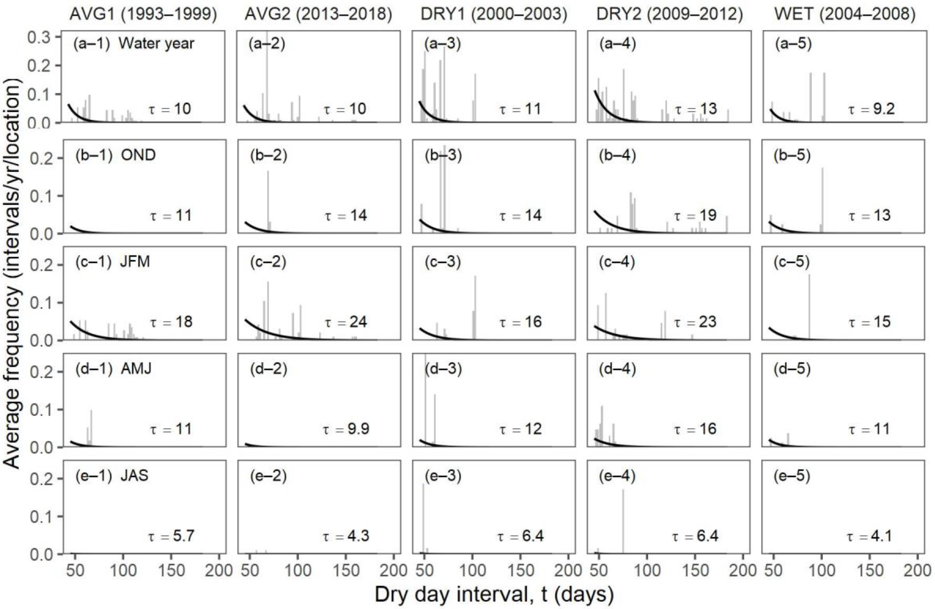
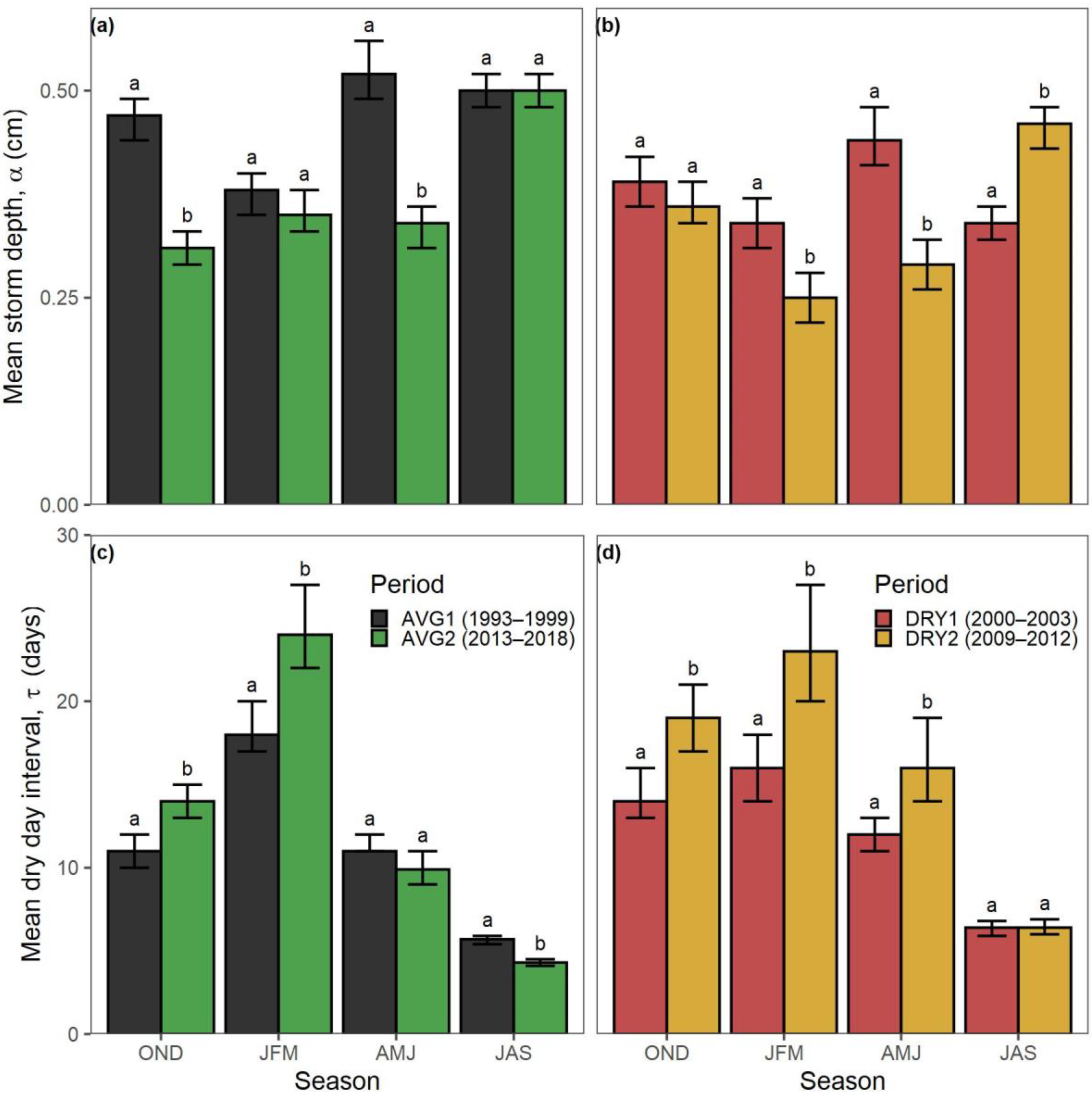
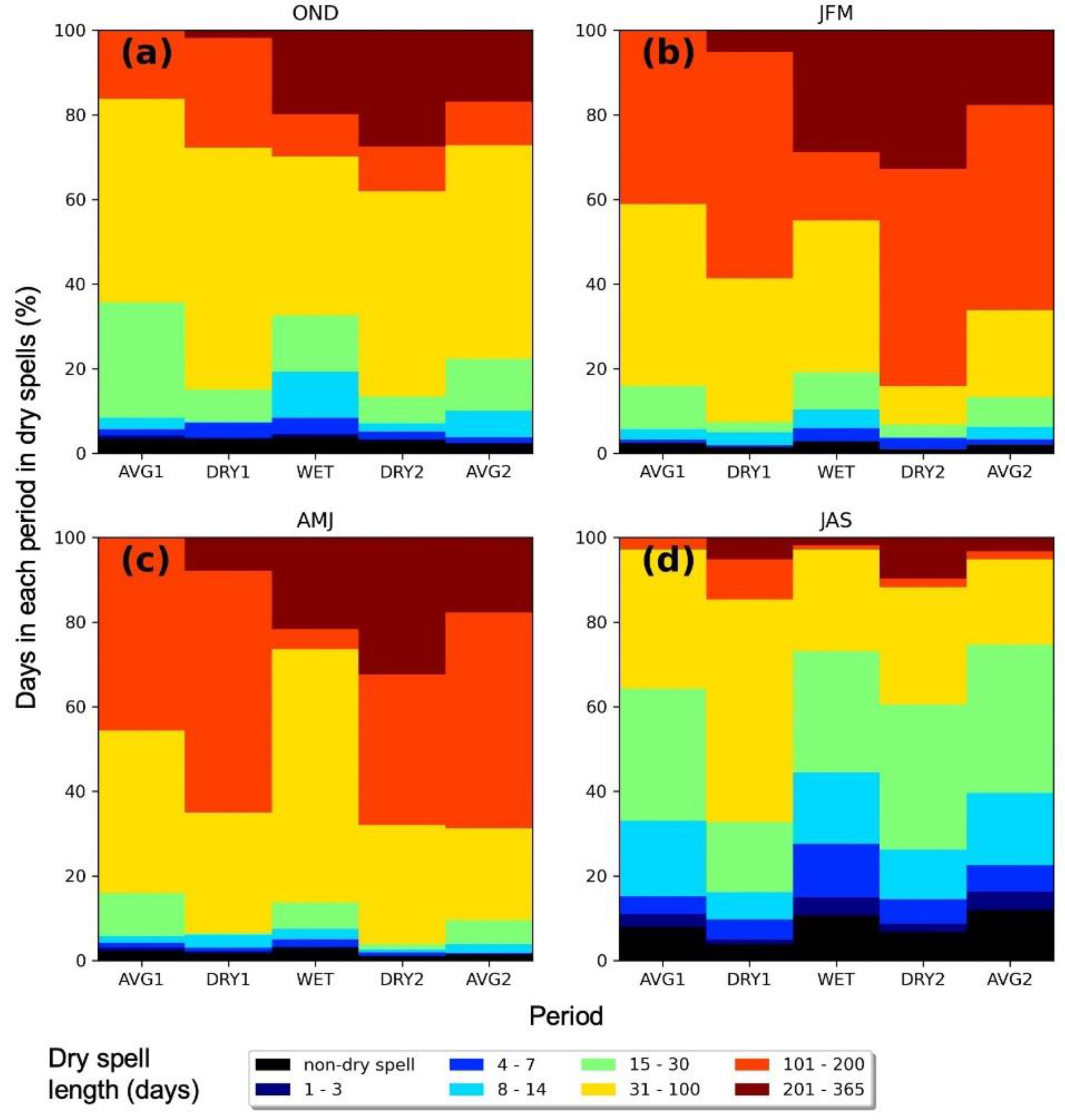
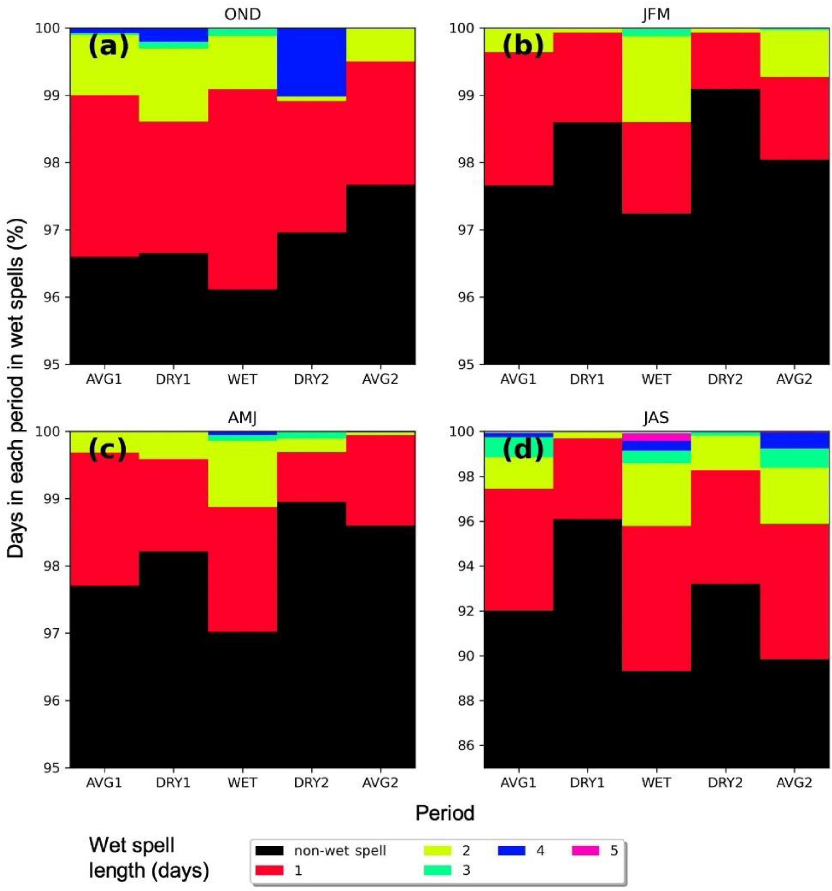
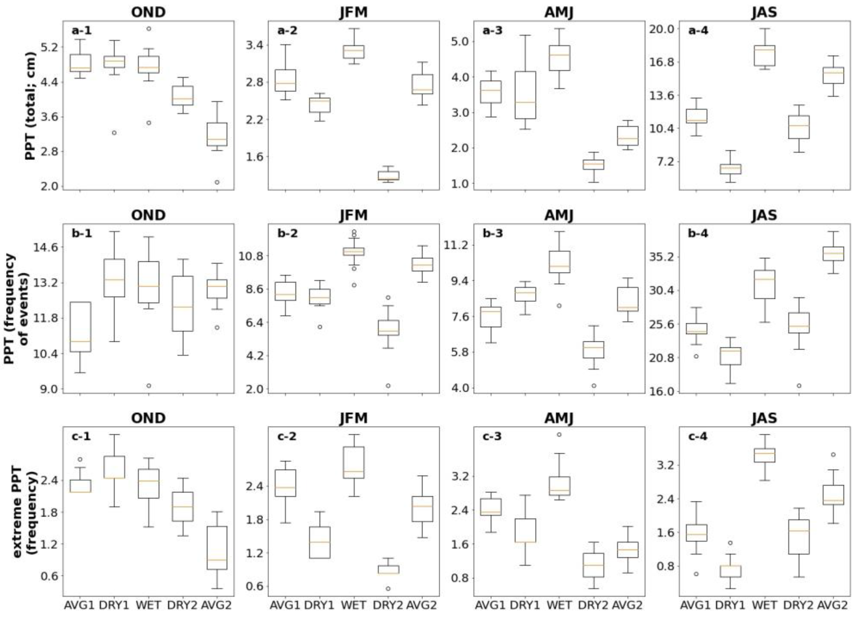
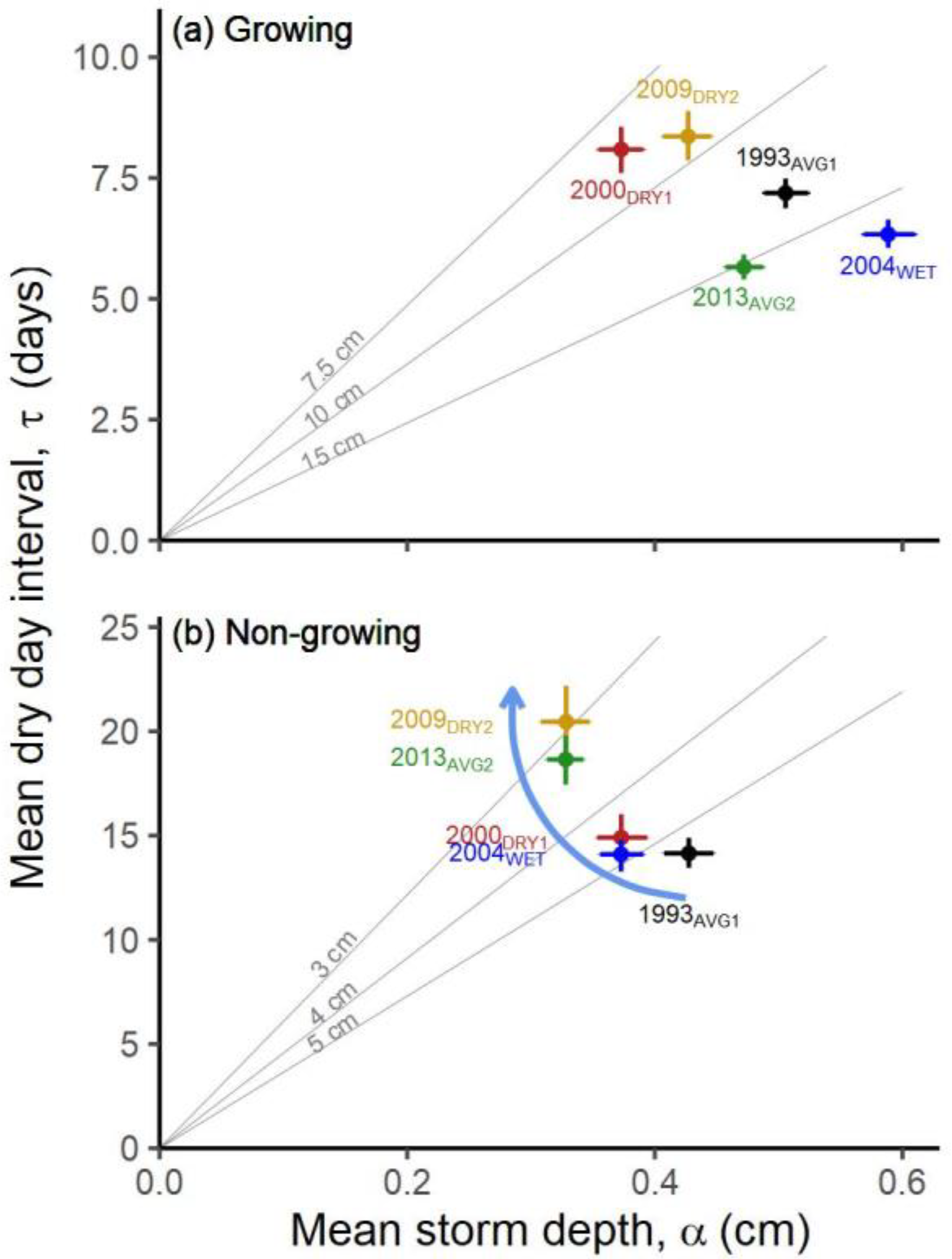
Figure 1. Water year precipitation (WPPT, cm) at n = 16 locations from 1993–2018 for five periods. (a) Periods delineated by breakpoint analysis (points for observed WPPT, horizontal lines for period means) compared with 89-year long-term mean (solid black horizontal line) and ± 0.5 standard deviation (black dashed lines). (b) WPPT means by periods with 95% confidence intervals and letters indicating significantly different means among periods from repeated measures ANOVA.
Climate 09 00130 g001
Figure 2. Species richness (number square meter) at four ecosystem types (columns, 14) for three functional groups and total combined (rows, ad). Period average richness and ±1-standard error shown. Letters indicate significantly different means in the five-way comparison of periods. Asterisks over DRY2 or AVG2 indicate significantly different means in pairwise comparisons with DRY1 or AVG1, respectively. Vertical scale differs by functional group.
Climate 09 00130 g002
Figure 3. Storm depth distributions (bars; relative number of days/yr/location) and fitted exponential PDFs (curves) for depths ≥3 cm with a bin size of 0.25 cm. Only nonzero precipitation is shown. Relative frequency for each season and period was calculated using bin frequency from all 16 locations and number of years in the period divided by 16 and the number of years. PDF curves (probability density) are vertically-scaled to match the average frequencies. Vertical scale differs by row. Row (a) is water year, row (b) is fall, row (c) is winter, row (d) is spring, and row (e) is summer.
Climate 09 00130 g003
Figure 4. As in Figure 3 except for depths ≥3 cm.
Climate 09 00130 g004
Figure 5. Dry-day interval sample distributions (bars; number of intervals/yr/location) and fitted exponential PDFs (curves) <45 days with a bin size of 2 days. Relative frequency for each season and period was calculated using bin frequencies from all 16 locations, number of years in the period divided by 16 and the number of years. PDF curves (probability density) are vertically-scaled to match the average frequencies. Row (a) is water year, row (b) is fall, row (c) is winter, row (d) is spring, and row (e) is summer.
Climate 09 00130 g005
Figure 6. As in Figure 5 except for dry-day intervals ≥45 days. Vertical scale differs by row.
Climate 09 00130 g006
Figure 7. Mean storm depth (a,b) and dry-day interval (c,d) by season for AVG1 vs. AVG2 (left) and DRY1 vs. DRY2 (right). Bar height denotes median bootstrapped parameter estimates, and error bars denote 95% confidence intervals for the estimates.
Climate 09 00130 g007
Figure 8. Percentage of days in each period in dry spells (consecutive days with less than 0.5 cm/day) of varying durations (days) as an average of 16 locations for each season. (a) OND, (b) JFM, (c) AMJ, and (d) JAS. Black bars represent the percentage of days not in a “dry spell” of at least one day.
Climate 09 00130 g008
Figure 9. Percentage of days in each period in wet periods of varying durations (days) as an average of 16 locations for each season. (a) OND, (b) JFM, (c) AMJ, and (d) JAS. Black bars represent the percentage of days not in a “wet period” of more than one day.
Climate 09 00130 g009
Figure 10. Period average of annual precipitation metrics by season: fall (OND), winter (JFM), spring (AMJ), and summer (JAS). Boxplots represent the distribution of values at the 16 locations. (a-1a-4) Total precipitation (cm), (b-1b-4) frequency of precipitation exceeding 0.01 cm/day (% of days), and (c-1c-4) frequency of precipitation exceeding the 98th percentile (% of days). Letters indicate significantly different means in the five-way comparison of periods. Vertical scales differ by season for each precipitation metric.
Climate 09 00130 g010
Figure 11. Mean storm depth (α) and mean dry-day interval (τ) combinations for the five periods during (a) growing season and (b) nongrowing season. Points indicate median estimated parameter values, and error bars indicate 95% confidence interval for the estimate. Periods are labeled with the first year in the period. Gray oblique lines represent α and τ combinations that result in equal mean seasonal total PPT.
Climate 09 00130 g011
Table 1. Summary of significant differences in richness or precipitation characteristics between periods with similar total amounts of precipitation 1. Counter-intuitive results are shown in red text. Figures are identified in column headers.
Ecosystem TypeFunctional Group (Relevant Season)Richness 1
[Figure 2]
Mean Storm Depth (Alpha)
[Figure 7a,b]
Mean Dry-Day Interval (Tau)
[Figure 7c,d]
Dry Spell Length (31–200 Days)
[Figure 8]
Wet Spell Length (>2 Days)
[Figure 9]
Total PPT 2
[Figure 10a]
PPT 2 Frequency
[Figure 10b]
Extreme PPT 2 Frequency
[Figure 10c]
Upland grasslandsC3 (AMJ)A1 > A2
D1 > D2
A1 > A2
D1 > D2
D1 < D2A1 < A2
D1 > D2
A1 > A2
D1 > D2
D1 > D2A1 > A2
D1 > D2
C4 (JAS)
Perennial grasses (JAS)
Creosote ShrublandsC3 (AMJ)A1 > A2A1 > A2 A1 < A2 A1 > A2 A1 > A2
C4 (JAS)D1 < D2D1 < D2 D1 > D2D1< D2D1 < D2D1 < D2D1 < D2
Perennial grasses (JAS)A1 > A2 A1 > A2A1 > A2A1 < A2A1 < A2A1 < A2A1 < A2
Mesquite ShrublandsC3 (AMJ)A1 > A2A1 > A2 A1 < A2 A1 > A2 A1 > A2
C4 (JAS)
Perennial grasses (JAS)
Tarbush ShrublandsC3 (AMJ)
C4 (JAS)
Perennial grasses (JAS)A1 > A2 A1 > A2A1 > A2A1 < A2A1 < A2A1 < A2A1 < A2
1 A1: AVG1; A2: AVG2; D1: DRY1; D2: DRY2 2 PPT = precipitation.
Publisher’s Note: MDPI stays neutral with regard to jurisdictional claims in published maps and institutional affiliations.

