Investigation of Numerical Dissipation in Classical and Implicit Large Eddy Simulations


Centre for Computational Engineering Sciences, Cranfield University, Cranfield, Bedfordshire MK43 0AL, UK
*
Author to whom correspondence should be addressed.
Aerospace 2017, 4(4), 59; https://0-doi-org.brum.beds.ac.uk/10.3390/aerospace4040059
Submission received: 21 November 2017
/
Revised: 6 December 2017
/
Accepted: 7 December 2017
/
Published: 11 December 2017
(This article belongs to the Special Issue Computational Aerodynamic Modeling of Aerospace Vehicles)
Abstract
:The quantitative measure of dissipative properties of different numerical schemes is crucial to computational methods in the field of aerospace applications. Therefore, the objective of the present study is to examine the resolving power of Monotonic Upwind Scheme for Conservation Laws (MUSCL) scheme with three different slope limiters: one second-order and two third-order used within the framework of Implicit Large Eddy Simulations (ILES). The performance of the dynamic Smagorinsky subgrid-scale model used in the classical Large Eddy Simulation (LES) approach is examined. The assessment of these schemes is of significant importance to understand the numerical dissipation that could affect the accuracy of the numerical solution. A modified equation analysis has been employed to the convective term of the fully-compressible Navier–Stokes equations to formulate an analytical expression of truncation error for the second-order upwind scheme. The contribution of second-order partial derivatives in the expression of truncation error showed that the effect of this numerical error could not be neglected compared to the total kinetic energy dissipation rate. Transitions from laminar to turbulent flow are visualized considering the inviscid Taylor–Green Vortex (TGV) test-case. The evolution in time of volumetrically-averaged kinetic energy and kinetic energy dissipation rate have been monitored for all numerical schemes and all grid levels. The dissipation mechanism has been compared to Direct Numerical Simulation (DNS) data found in the literature at different Reynolds numbers. We found that the resolving power and the symmetry breaking property are enhanced with finer grid resolutions. The production of vorticity has been observed in terms of enstrophy and effective viscosity. The instantaneous kinetic energy spectrum has been computed using a three-dimensional Fast Fourier Transform (FFT). All combinations of numerical methods produce a spectrum at , and near the dissipation peak, all methods were capable of predicting the slope accurately when refining the mesh.
1. Introduction
The complexity of modelling turbulent flows is perhaps best illustrated by the wide variety of approaches that are still being developed in the turbulence modelling community. The Reynolds-Averaged Navier–Stokes (RANS) approach is the most popular tool used in industry for the study of turbulent flows. RANS is based on the idea of dividing the instantaneous parameters into fluctuations and mean values. The Reynolds stresses that appear in the conservation laws need to be modelled using semi-empirical turbulence models. Direct Numerical Simulation (DNS) is another approach used to study turbulent flows where all the scales of motion are resolved. It should be noted that even using the highest performance computers, it is very difficult to study high Reynolds number flows directly by resolving all the turbulent eddies in space and time. An alternative approach is Large Eddy Simulation (LES), where the large scales or the energy-containing scales are resolved and the small scales that are characterised by a universal behaviour are modelled. A subgrid-scale tensor must be included to ensure the closure of the system of governing equations. This process reduces the degrees of freedom of the system of equations that must be solved and reduces the computational cost. Implicit Large Eddy Simulation (ILES) is an unconventional LES approach developed by Boris in 1959 [1]. The main idea behind this approach is that no subgrid scale models are used, and the effects of small scales are incorporated in the dissipation of a class of high-order non-oscillatory finite-volume numerical schemes. The latter are characterised by an inherent numerical dissipation that plays the role of an implicit subgrid-scale model that emulates and models the small scales of motion. ILES has not yet received a widespread acceptance in the turbulence modelling community due to the lack of a theoretical basis that proves this approach. In addition to that, pioneers of ILES have worked in a very isolated way unaware of each others’ work, which made it difficult to understand the main elements of this approach. Thus, many research groups are using ILES nowadays and are validating it against benchmark test cases, which gives this approach more credibility in many applications.
ILES is an advanced turbulence modelling approach due to its ease of implementation and since it is not based on any explicit Subgrid-Scale (SGS) modelling, which could reduce computational costs. Moreover, the fact that no SGS model is used prevents any modelling errors that affect the accuracy of the numerical solution, in contrast with the explicit large eddy simulation approach where modelling, differentiation and aliasing errors can have impacts on the numerical solution. In addition to that, non-oscillatory finite volume numerical schemes used within the framework of the ILES approach are computationally efficient and parameter free, which means that they do not need to be adapted and modified from one application to another [2]. It should be noted that even if the classical approach to ILES is based on using the inherent dissipation of the convective term as an implicit subgrid-scale model, a recent approach presented an alternative way to perform ILES by a controlled numerical dissipation that is included in the discretisation of the viscous terms through a modified wavenumber used in the evaluation of the second-derivatives in the framework of the finite difference method. The latter approach showed very accurate results compared to DNS data in [3]. This is an indicator of the efficiency of the ILES approach, which is fully independent of modelling of small scales.
Large eddy simulation is becoming widely used in many fundamental research and industrial design applications. Despite this positive situation, LES suffers from weaknesses in its formalism, which make this approach questionable since the mathematical formulation of the LES governing equations is just a model of what is applied in a real LES. In practice, the removal of small scales is carried out by a resolution truncation in space and time along with numerical errors that are not well understood. In LES, a significant part of numerical dissipation is ensured by the subgrid-scale model. However, a truncation error is induced by the mesh resolution and the computational methods being used, and the vast majority of LES studies do not consider this truncation error. The latter should not be neglected since it could overwhelm the subgrid-scale model effect when dissipative numerical methods are used. Sometimes, discretisation and modelling errors cancel each other leading to an increase in the accuracy of the numerical solution, but still, the fact that the truncation error is neglected should be questioned [4]. This conclusion was pointed out in the study carried out by Chow and Moin [5], who showed through a statistical analysis that the truncation error could be comparable and higher than the subgrid-scale error when the grid resolution is equal to the filter width . Moreover, based on the idea that modelling and truncation errors could cancel each other, some studies pointed out an optimal grid resolution that reduces the numerical errors when the study is not connected to a subgrid-scale model like the Smagorinsky model. The conclusion drawn is that using a grid size less than the filter width allows the control of the truncation error. Unfortunately, this recommendation is rarely followed in the literature [6]. Most LES users are aware of this truncation error, but their conjecture is that it does not affect seriously the results in a wide range of applications. The term “seriously” should be a subject of debate in order to build an awareness of the effect of numerical errors on the accuracy of the solution. ILES suffers as well from some weaknesses that made this approach still be argued about by some scientists. Even if ILES is capable of reproducing the dynamics of Navier–Stokes equations, quantitative studies showed that the numerical dissipation inherent in a class of high-order finite volume numerical schemes could be higher than the subgrid-scale dissipation, which leads to poor results. Another scenario is that the numerical dissipation is smaller than the SGS dissipation yielding good results only in short time integrations. Poor-quality results are obtained in long time integrations due to energy accumulation in high wave numbers [7,8]. Accordingly, there is no clear mechanism to ensure the correct amount of numerical dissipation that should match the SGS dissipation. ILES is often considered as under-resolved DNS; however, ILES terminology should be reserved only for schemes that reproduce the correct amount of numerical dissipation.
Since LES and ILES techniques are often used for modelling mixing processes, therefore the quantitative measure and estimate on the numerical dissipation and dispersion are crucial. Research work on this subject is carried out by other authors, because the quantification of the dissipative properties of different numerical schemes is at the centre of interest in the field of computational physics and engineering sciences. Bonelli et al. [9] carried out a comprehensive investigation of how a high density ratio does affect the near- and intermediate-field of hydrogen jets at high Reynolds numbers. They developed a novel Localized Artificial Diffusivity (LAD) model to take into account all unresolved sub-grid scales and avoid numerical instabilities of the LES approach. In an earlier work, Cook [10] focused on the artificial fluid properties of the LES method in conjunction with compressible turbulent mixing processes dealing with the modified transport coefficients to damp out all high wavenumber modes close to the resolution limit without influencing lower modes. Cook [10] used a tenth-order compact scheme during the numerical investigations. Kawai and Lele [11] simulated jet mixing in supersonic cross-flows with the LES method using an LAD scheme. Their paper devotes particular attention to the analysis of fluid flow physics relying on the computational data extracted from the LES results. De Wiart et al. [12] focused on free and wall-bounded turbulent flows within the framework of a Discontinuous Galerkin (DG)/symmetric interior penalty method-based ILES technique. Aspden et al. [13] carried out a detailed mathematical analysis of the properties of the ILES techniques comparing simulation results against DNS and LES data. The aforementioned contributions made attempts to obtain very accurate results within the framework of LES and ILES methods to gain a deeper insight into the behaviour of the physics of turbulence. The reader can refer to the application of the ILES method in different contexts [14,15,16,17,18], where the quantification of numerical dissipation and dispersion could also be employed to improve the accuracy of the numerical solution.
Due to the above-described reasons, quantifying the numerical dissipation that is inherent in numerical schemes is of great importance to investigate the effect of truncation error on the accuracy of the results. The aim is to examine if the subgrid-scale model is providing the correct amount of dissipation to model the small scales, or otherwise, the contribution of truncation error to the numerical dissipation has a significant effect that could not be neglected, as was done in most large eddy simulation studies. Proving that the truncation error could not be ignored would allow one to work on controlling the effect of numerical dissipation inherent in the scheme in order to predict and provide the correct amount of dissipation needed for modelling the small scales of motion correctly. It should be reminded that the dissipation induced in the numerical methods used within the framework of the ILES approach to act as a subgrid-scale model is mainly related to the convective term of Navier–Stokes equations. Thus, investigating the discretisation error induced in the convective term of the fully-compressible Navier–Stokes equations is a prime objective in this study.
The contribution of truncation error induced in the convective term to the total numerical dissipation of the solution will be evaluated using Modified Equation Analysis (MEA). This approach consists of deriving a modified version of the partial differential equation to which the truncation error of the numerical scheme used to discretize the PDE is added. The MEA approach is based on Taylor series expansions of each component of the discretized convective term. This methodology is inspired by the linear approach introduced in the book of Fletcher in 1988 [19] where the MEA is applied to 1D linear equations. This approach is extended and applied to the three-dimensional Navier–Stokes equations during the course of this study. Since the modified equation analysis needs a substantial amount of algebraic manipulations, the solution-dependent coefficients multiplying the derivatives in the convective term are considered to be frozen as explained in [19]. This approximation works well and gives good results despite the lack of a theoretical basis to prove it. The Taylor–Green Vortex (TGV) is a benchmark test case that matches the aims of this paper. It helps with understanding the transition mechanism for turbulence and small scales’ production. Moreover, TGV allows the investigation of the resolving power of the numerical scheme, which is represented by its ability to capture the physical features of the flow. The inviscid Taylor–Green vortex is used within the framework of this study to understand the inherent numerical dissipation of the MUSCL scheme with different slope limiters and the dissipation of the dynamic Smagorinsky subgrid-scale model.
2. Numerical Model and Flow Diagnostics
The dynamics of Taylor–Green Vortex (TGV) are investigated in terms of classical, and implicit large eddy simulation and comparisons with high-fidelity DNS data provided in the study of Brachet et al. [20,21] are performed. The Taylor–Green vortex is considered as a canonical prototype for vortex stretching and small-scale eddies’ production. The TGV flow is initialized with solenoidal velocity components represented in the following initial conditions as:
The initial pressure field is given by the solution of a Poisson equation for the given velocity components and could be represented as:
where k represents the wavenumber and a value is adopted in accordance with the study carried out by Brachet et al. [20]. An ideal gas characterised by a Mach number is considered. For this specified Mach number, compressible effects could be expected since that value falls within the range of mild compressible flows or near incompressible conditions. The initial setup yields the following values for the initial flow parameters:
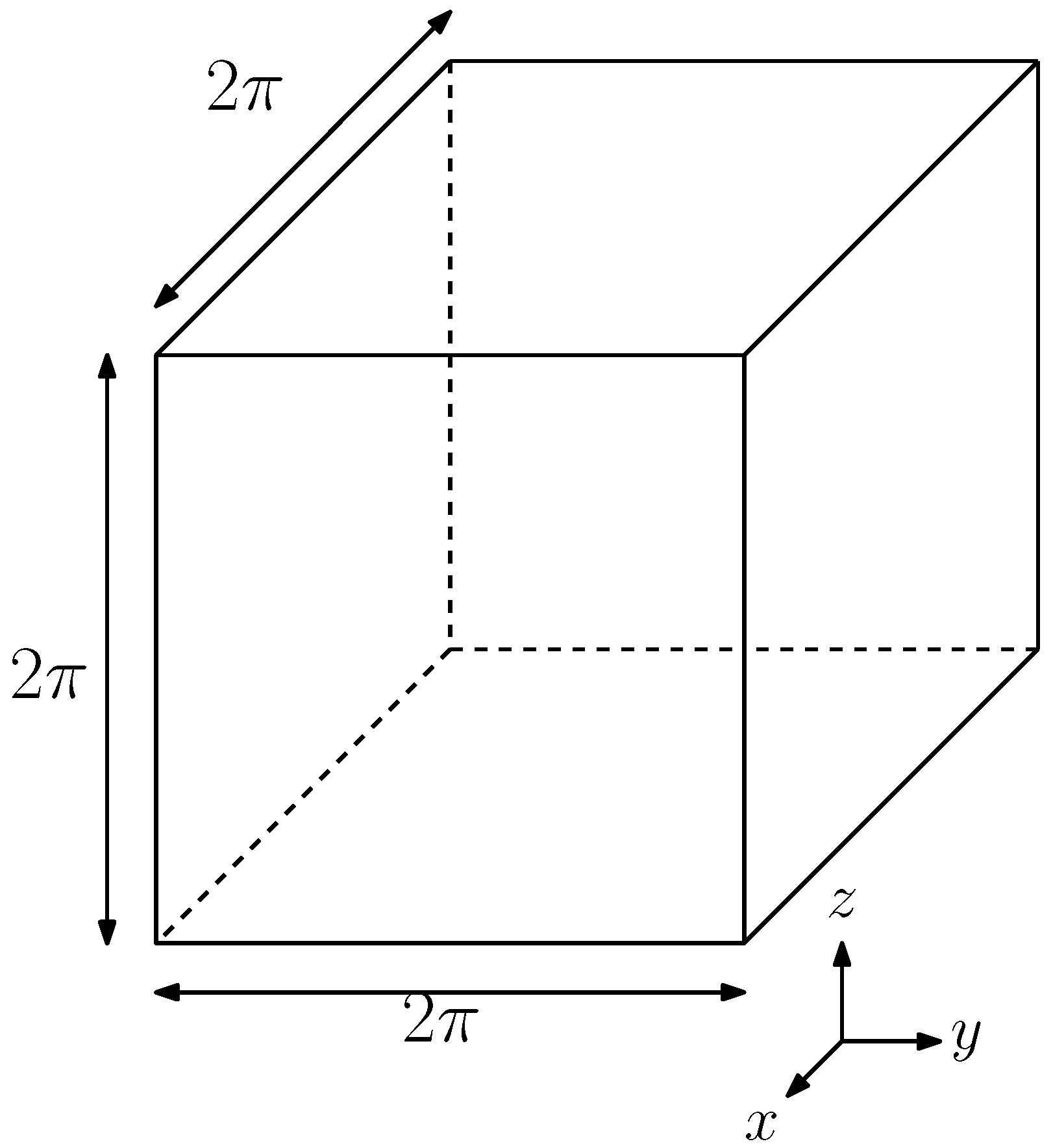
All the results are given in non-dimensional form where for example is the non-dimensional time and represents a non-dimensional distance. ILES were performed using a fully-compressible explicit finite volume method-based in-house code, which was developed within postgraduate research projects. The Harten–Lax–van Leer–Contact (HLLC) Riemann solver was adopted for the present study, and the MUSCL third-order scheme with three-different slope limiters was employed for spatial discretisation. In addition to this, the ANSYS-FLUENT solver is adopted for the classical LES considering the dynamic Smagorinsky subgrid-scale model and the third-order MUSCL scheme for spatial discretisation. The reason for employing the MUSCL third-order scheme in the in-house code is to be consistent with the FLUENT solver in terms of the order of accuracy. For improving the accuracy of the time-integration, a second-order strong stability preserving Runge–Kutta scheme [22,23] has been employed. In the simulation setup, the box of edge length is considered as the geometry for the problem as shown in Figure 1 where the outer domain is located at . This specific configuration of the Taylor–Green vortex allows triply periodic boundary conditions at the box interfaces.
The initial problem has eight-fold symmetry, and the computations could be just considered on 1/8 of the domain, which can significantly reduce the computational cost. However, using symmetry conditions at the interfaces prevents the symmetry breaking property, which characterises the numerical scheme. Symmetry breaking means that the flow starts with symmetry and ends up with a non-symmetrical state; thus, if only 1/8 of the domain is studied, the resolving power of the numerical scheme cannot be assessed in a valid and credible way.
A block-structured Cartesian mesh topology was adopted for the discretisation of the computational domain utilized for the ILES and LES approaches. In regards to the ILES, three grid levels where created having , and cells. The extrapolation methods employed for the simulations are the second-order MUSCL scheme with Van Albada slope limiter (M2-VA), the third-order MUSCL with Kim and Kim limiter [24] (M3-KK), and the third-order MUSCL scheme with the Drikakis and Zoltak limiter [25] (M3-DD). The second-order strong stability-preserving Runge–Kutta scheme is used for temporal discretisation for the ILES approach. It has been demonstrated that the time discretisation method has only a minor effect on the results obtained using the MUSCL scheme, and for this reason, the previously-mentioned time integration scheme was employed for the simulations since it allows the use of higher Courant–Friedrichs–Lewy (CFL) numbers while preserving the stability [26]. A CFL = 0.8 was employed for all the numerical schemes, which induces equal time steps at each grid level.
In regards to the classical LES, the dynamic Smagorinsky subgrid-scale model is adopted, and the third-order MUSCL scheme (M3) is chosen for spatial discretisation. The latter is built in FLUENT as the sum of upwind and central differencing schemes where an under-relaxation factor is introduced to damp spurious oscillations. The derivation of the MUSCL scheme and the Dynamic Smagorinsky (DSMG) subgrid-scale (SGS) model used in FLUENT are not presented in this study. It should be noted that the simulations were performed using the density-based solver, and the Roe–Riemann solver is considered for the flux evaluation at the cell interfaces. Three grid levels were generated having , and cells. One could see that the finest LES grid is much finer than the finest grid used within the ILES approach. The mesh will allow the more in depth study of the dynamics of TGV and the investigation of the grid refinement effect on the performance of the SGS model.
As mentioned earlier, the Taylor–Green vortex is a very good test case that allows the study of a numerical scheme’s resolving power. The dynamics encountered during the flow evolution in time characterize the behaviour of the numerical scheme being investigated. Hence, several integral quantities have been calculated for the diagnostics of the TGV flow. Nevertheless, some of these quantities are based on the assumption of homogeneous and isotropic turbulence, which is not applied to all phases of Taylor–Green vortex flow evolution. However, investigating those parameters gives a more comprehensive idea about the characteristics of the flow. The volume-averaged kinetic energy can be used as an indicator of the dissipation or the loss of conservation that is related to the numerics being used for the discretisation of the governing equations.
The volume-averaged kinetic energy is defined in an integral form as:
where V is the volume of the domain. The kinetic energy could be written in a more compact way as:
where will be used in the rest of this paper to represent the volumetric average of a given quantity. In theory, the kinetic energy should be conserved during the evolution of the flow if the latter is inviscid or for very small viscosity values, since no viscous effects are present to damp the kinetic energy into heat. The assumption of energy conservation holds only when the numerical scheme is able to conserve the kinetic energy or when all the scales of motion could be resolved. Hence, the decay of kinetic energy helps with indicating the onset or the exact time where the flow becomes under-resolved.
The kinetic energy dissipation rate is an important parameter that can be used to quantify the decay of kinetic energy in time and is representative of the slope of the volumetric average kinetic energy development. This parameter is defined as:
The production of vorticity could be monitored in terms of enstrophy, which is comparable to the kinetic energy dissipation. The enstrophy should grow to infinity when considering an inviscid flow. Therefore, the behaviour or the evolution of enstrophy can be considered as one of the criteria that are used to assess the resolving power of a numerical scheme and its ability to predict the flow physics accurately. The enstrophy is simply the square of vorticity magnitude and can be expressed as:
For compressible flows, the dissipation of kinetic energy is the sum of two other components given by:
where is the strain rate tensor. The pressure dilatation-based dissipation is expected to be small in the incompressible limit, and hence, it is neglected during this study. Furthermore, for high Reynolds number flows, the volumetric average of the strain rate tensor product is equal to the enstrophy as derived in [27]. Hence, the dissipation rate could be finally expressed as:
where is the effective viscosity that represents the viscosity related to the dissipation of kinetic energy, and it is equal to the mean viscous dissipation.
The kinetic energy spectrum is represented for all the numerical methods, as well. Representing the three-dimensional kinetic energy spectra for the Taylor–Green vortex is useful to obtain a deeper understanding of kinetic energy distribution within all the scales of motion numerically resolved. The aim is to investigate whether the TGV presents an inertial subrange or not as predicted by Kolmogorov [28], who found that for homogeneous and isotropic turbulence, the kinetic energy spectrum follows a slope in the inertial subrange, where k is the wavenumber. The three-dimensional velocity components are considered for the computation of the energy spectrum, which means that the three-dimensional array of the problem is considered. It should be reminded that the Taylor–Green vortex has an eight-fold symmetry, and some researchers use 1/8 of the domain size to calculate the energy spectra; but for the purpose of this study, all of the domain was considered. A three-dimensional Fast Fourier Transform (FFT) of the velocity components should give a three-dimensional array of amplitudes, which represent the Fourier modes corresponding to wavenumbers . By summation of the FFT square of each velocity component, a three-dimensional array containing the kinetic energy spectrum components is obtained. In the next step, a spherical integration of the three-dimensional array of the spectrum is carried out to obtain a 1D array that represents the kinetic energy spectrum, which is plotted versus the total wave number defined as .
The spherical integral could be expressed as:
where A is the three-dimensional array of Fourier modes’ amplitude, and L is the characteristic length. The TGV is a well-established computational benchmark to investigate the dissipative and dispersive properties of various numerical schemes, and one can find more details about this research area in conjunction with numerical investigations in [29,30,31,32].
3. Results and Discussions
3.1. Taylor–Green Vortex Flow Topology
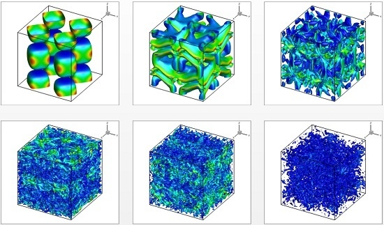
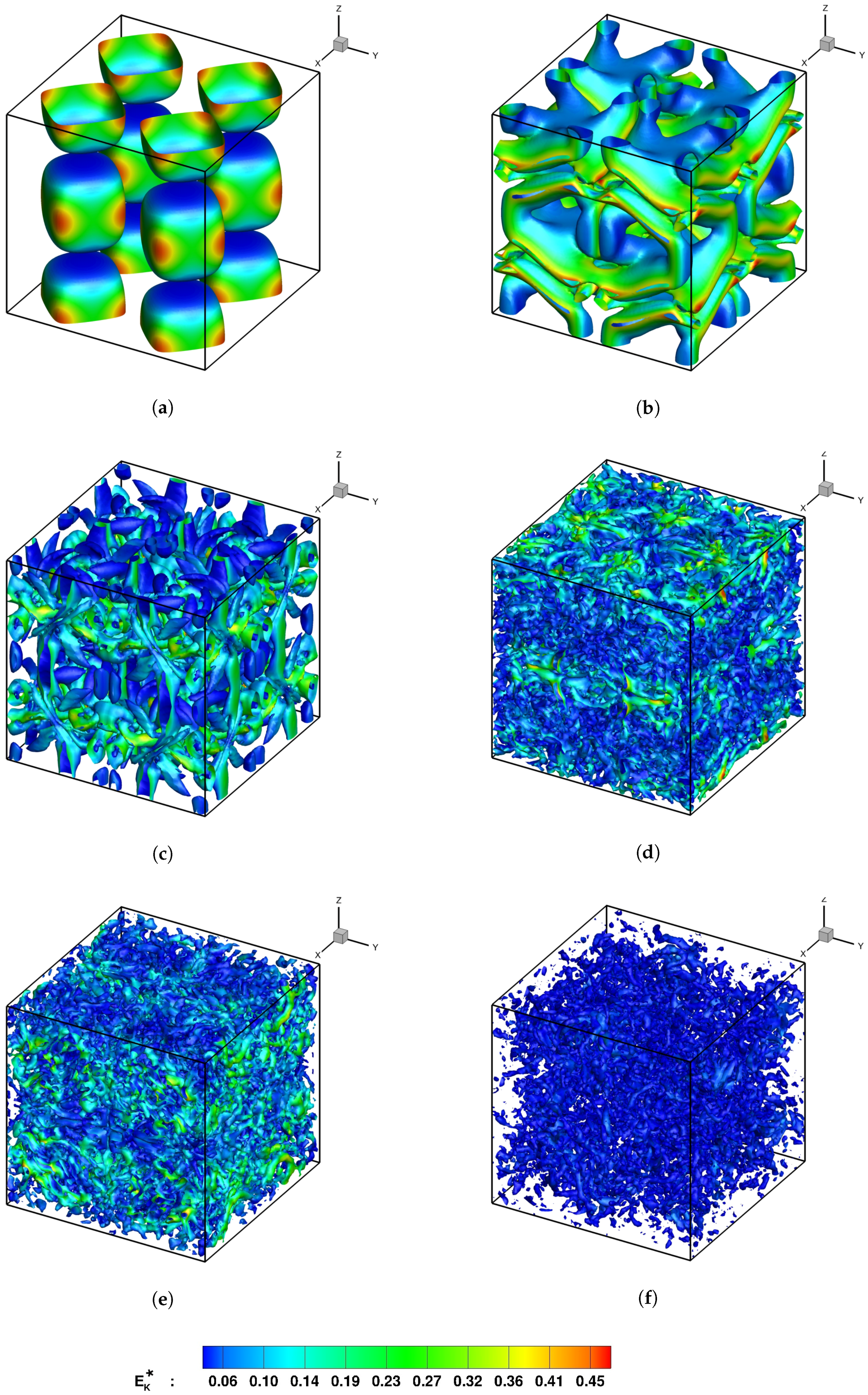
This section is devoted to the discussion of the dynamics of the Taylor–Green vortex. The flow topology is investigated qualitatively on the basis of the results obtained using the third-order MUSCL scheme with the Kim and Kim slope limiter [24] and a grid size of cells. The flow is visualized using isosurfaces of a constant Q-criterion (see Figure 2). M3-KK is representative of all the other schemes that will generate similar contours, and the kinetic energy is represented in a dimensionless form in Figure 2. The eight-fold symmetry of the Taylor–Green vortex is clearly visible in Figure 2a, where the initial two-dimensional vorticity field features a symmetry in all planes located at a distance in the computational domain. No signs of vorticity are predicted at the intersection of the symmetry planes, and the highest vorticity magnitude values were predicted at the centre of the large structures represented by Q-criterion isosurfaces as described in the study carried out by Brachet et al. [20].
When the flow evolves, the vortices begin there descent to the symmetry planes, and vortex sheets are generated, as shown in Figure 2b. At this time stage, the flow starts to become under-resolved, and the kinetic energy can no longer be preserved. As the flow evolves more, the vortex sheet undergoes an instability and loses its coherent structure as presented in Figure 2c. After the disintegration of the vortex sheet due to the instability that was observed at earlier stages, the dynamics of TGV are governed by the interactions of small-scale structures of vorticity that are generated due to vortex stretching characterised by vortex tearing and re-connection. At late stages represented in Figure 2e, the flow becomes extremely disorganized, has no memory of the initial condition that was imposed and the symmetry is no longer maintained. Hence, the symmetry-breaking property that characterizes a numerical scheme is well observed by investigating the TGV flow topology, since the flow starts with a symmetry and ends up non-symmetric. At very late stages, the worm-like vortices fade away (see Figure 2f), and this behaviour is very similar to homogeneously decaying turbulence.
3.2. Effect of Grid Resolution
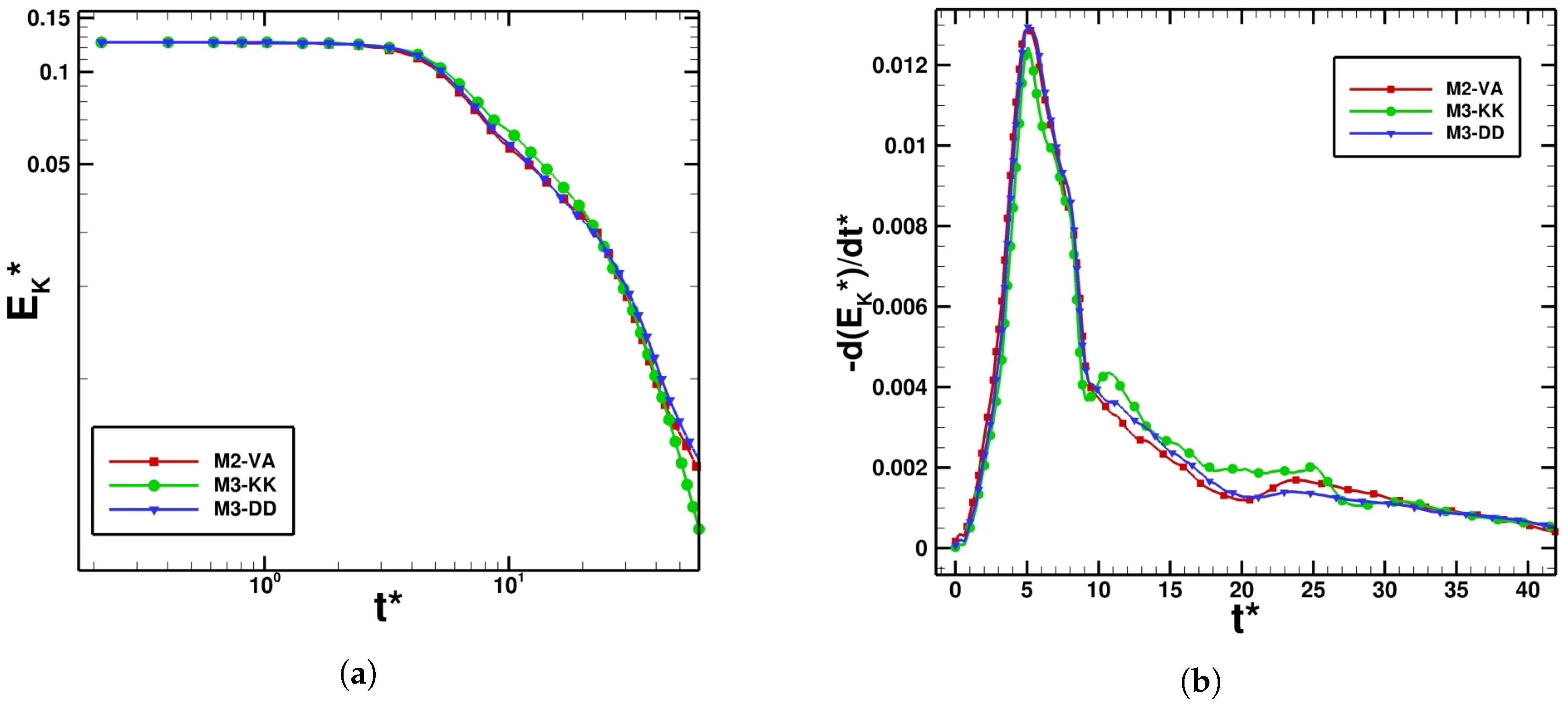
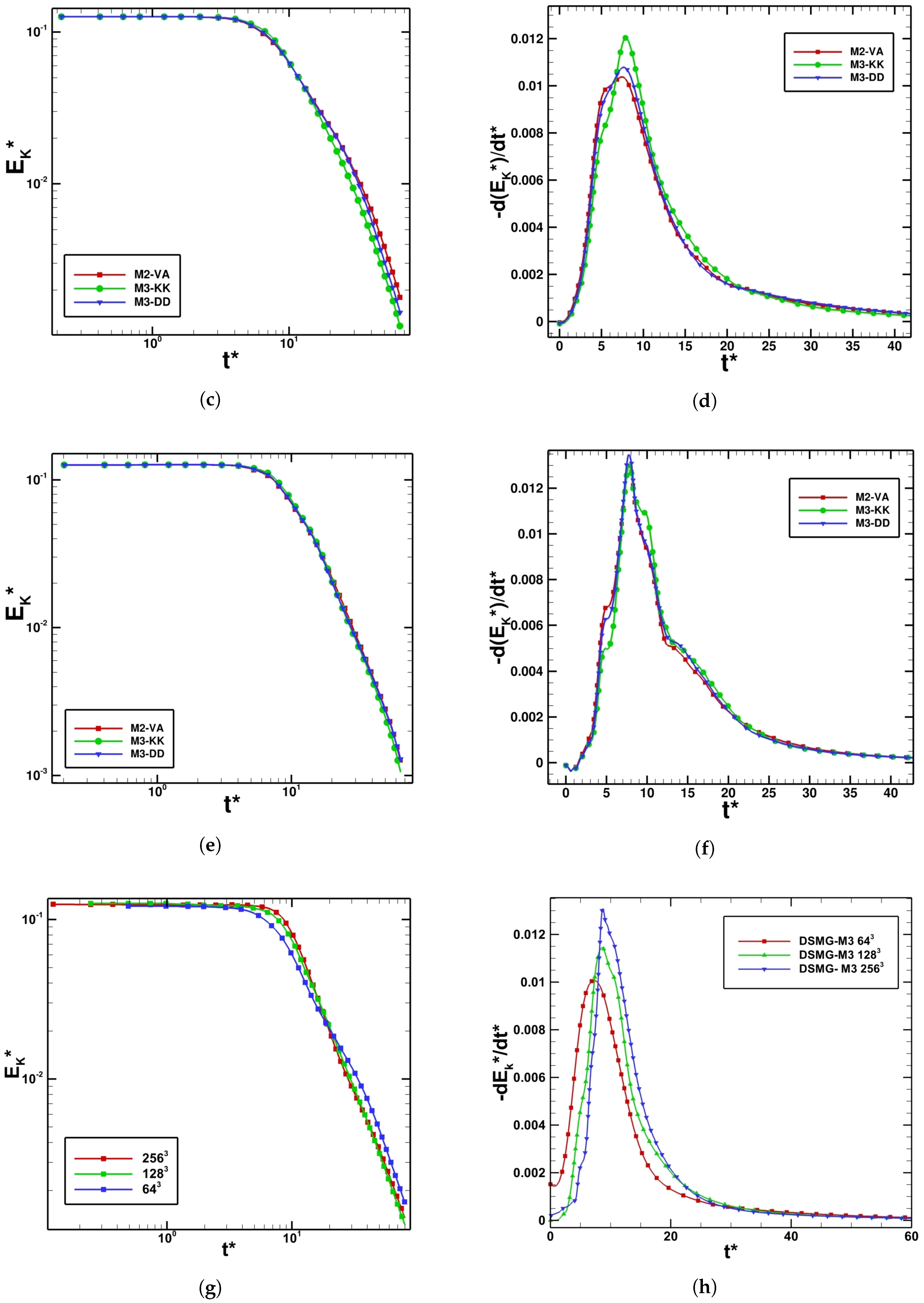
The dynamics of the Taylor–Green vortex are directly dependent on the resolving power of the numerical scheme and the grid size adopted. In order to assess the effect of grid resolutions on the evolution of TGV flow, simulations were performed using second and third-order MUSCL schemes (M2-VA, M3-KK and M3-DD) considering three levels of grids having sizes of , and cells. It should be noted that the second-order strong-stability preserving Runge–Kutta scheme has been utilized for temporal discretisation. The same grid refinement study was performed using the dynamic Smagorinsky subgrid-scale model and third-order MUSCL scheme (DSMG-M3) on , and grids. The differences in the flow dynamics during the time evolution of the simulation are of great interest to understand the effect of mesh size on the performance of the numerical scheme or the SGS model. Figure 3 shows the evolution of volumetrically-averaged dimensionless kinetic energy and kinetic energy dissipation rate for all the numerical methods and all grid levels used within this study.
The kinetic energy is represented in logarithmic scale to understand the trend line that the kinetic energy decay follows. In theory, the kinetic energy for an inviscid flow should be conserved since no viscous effects are present to damp it into heat. However, it is obvious that the latter is decaying during the coarse of the simulations. The decay starts at the end of the laminar stage when the vortex sheet is generated and the flow becomes under-resolved. The kinetic energy dissipation increases due to the instability that the vortex sheet undergoes and to the formation of a smaller and smaller vortical tube. The DNS study performed by Brachet et al. [20,21] predicted that the kinetic energy reaches its dissipation peak at a non-dimensional time level . The time level at which the dissipation reaches its highest value is more or less predicted correctly by all the numerical schemes with the exception of DSMG-M3, which underpredicted that time level compared to the other schemes. At a time level higher than , the kinetic energy dissipation decreases rapidly and reaches a value of zero at very late time stages, and this behaviour is similar to homogeneously-decaying turbulence. The kinetic energy dissipation rate trend obtained on the mesh shows a non-physical behaviour predicted by all the numerical schemes used within the framework of the ILES approach. At late stages, when the flow becomes highly-disorganized (), all the numerical schemes predicted an increase in the dissipation of kinetic energy, which created a sort of hump in the trend of . In addition to that, the M3-KK scheme predicted an earlier increase in the kinetic energy dissipation at , which indicates a lower resolving power of that scheme compared to the other methods. Using finer grid resolutions, this non-physical behaviour vanishes, and the decay of kinetic energy at the stages when the flow is fully disorganized is pretty smooth. One could observe that this non-physical trend of kinetic energy dissipation rate was not observed in LES even on the coarsest grid. The dissipation peak represented by DSMG-M3 on a 64 mesh appears prior to the peak predicted on finer grids, which indicates that the onset of kinetic energy dissipation is happening earlier on a 64 grid. Refining the mesh, the kinetic energy plot represented in Figure 3g is more conserved since the volumetrically-averaged kinetic energy decay starts later on 128 and 256 grids compared to the coarsest grid, as observed qualitatively. The conclusion that could be drawn from the observation of kinetic energy and the kinetic energy dissipation rate is that the resolving power of the numerical scheme increases using finer grid resolutions. Note that mesh refinement increases the computational cost, which might become quite expensive for very fine grid resolutions. Both the ILES and LES approaches predicted similar dynamics of TGV, which indicates that the numerical dissipation inherent in high-order non-oscillatory numerical schemes could act as an implicit subgrid-scale model in predicting the flow features of homogeneously-decaying turbulence. As mentioned earlier, the kinetic energy is represented in a logarithmic scale in order to understand the trend line of the evolution of kinetic energy in time. It is obvious from Figure 3a,c,e,g that the kinetic energy follows a power law in time. This trend is similar to homogeneous and isotropic turbulence, where Kolmogorov [28] showed that the kinetic energy decay obeys a power law in time as:
where represents the onset of kinetic energy decay and P is the power that was evaluated by Kolmogorov and equal to . If the length of the largest scales of motion present in the flow are comparable to the grid resolution, the kinetic energy decays following a power law with , as shown in [33]. In this study, the decay exponent P is determined using curve fitting of kinetic energy data between and and values obtained for all numerical methods (see Table 1 and Table 2).
The decay exponent predicted by the numerical schemes used within the ILES approach on and grids falls in the range of the value predicted in [33] (). The value of P is underpredicted by all the numerical methods on the coarsest mesh ( cells), and it was similar to the value of the decay exponent predicted for homogeneous turbulence by Kolmogorov [28]. However, even if the values of P predicted by the coarsest mesh are close to the decay exponent of homogeneous and isotropic turbulence, one should not forget that a non-physical hump was observed in the volumetrically-averaged kinetic energy evolution, which makes the prediction of the decay slope erroneous. Without the presence of this “artificial” hump, the slope of decay would be steeper, and that could explain why the value of P was underpredicted. Refining the mesh, the hump vanishes, and the decay exponent converges to a value similar to the theoretical value provided by Skrbek and Stalp [33]. In regards to LES, it is obvious that the decay exponent obtained on a grid is lower than the slope predicted by the medium and fine mesh, which converges to two.
The onset is a very important parameter to understand and examine the resolving power of each numerical scheme. The more the kinetic energy is conserved, or in other words, the higher the onset of decay, the better the scheme is in terms of performance. It is obvious from Table 1 that M2-VA starts loosing kinetic energy before M3-DD, and the latter looses energy before M3-KK, which predicts the highest decay onset. Refining the mesh, the kinetic energy is more conserved, and hence, the performance of the numerical scheme is increased. The time at which the kinetic energy starts to decay is shown in Table 2 for the LES. Large differences of decay onset between the coarse, medium and fine grids are clear, and that could explain why the peak in the energy dissipation on the grid appears earlier in Figure 3h. Refining the mesh, the onset of decay increases significantly and reaches a value of 4.296 on the mesh, which indicates that the kinetic energy is best conserved on the finest grid. Compared to ILES results on a grid, the onset of decay predicted by LES is nearly half the values predicted by all numerical schemes (see Table 1), which means that DSMG-M3 looses kinetic energy faster than the high-order non-oscillatory finite volume numerical schemes used for ILES, and the flow becomes under-resolved earlier as predicted by DSMG-M3.
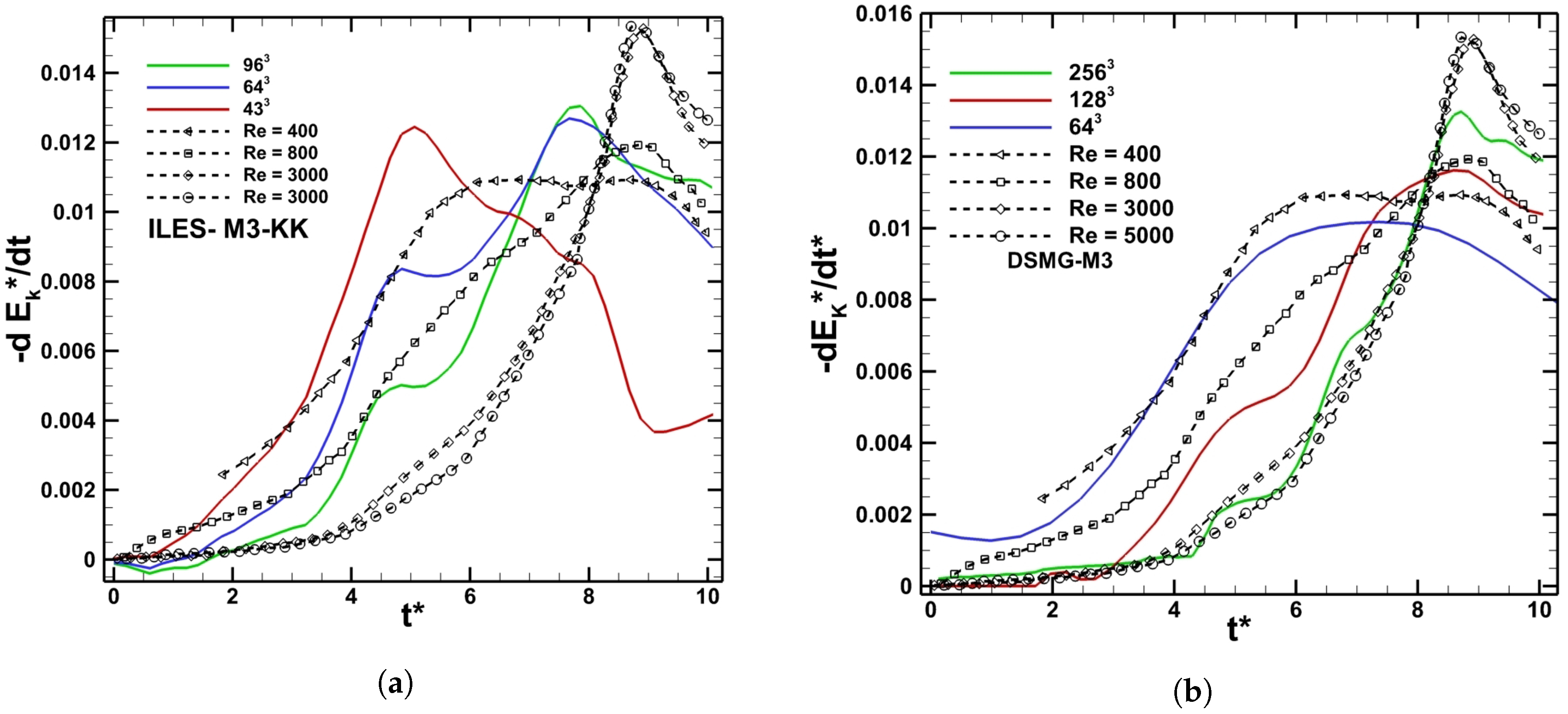
Studies of grid sensitivity of ILES and LES were carried out on all the grids generated and compared to DNS data provided in the study of Brachet et al. [20,21] for Re , 800, 3000 and 5000. It should be noted that explicit data for different Reynolds numbers are not available for the ILES and LES approaches, but the trend of kinetic energy dissipation rate will be used to observe the evolution of kinetic energy dissipation, as will be presented in Figure 4, compared to DNS results, which present the effects of physical viscosity, which damps the kinetic energy into heat. The DNS study showed that at high Reynolds number (Re ), the peaks of the kinetic energy dissipation rate remain identical, which means that the dissipation of kinetic energy reaches a Reynolds independent limit. By increasing the Reynolds number above this limit, the dissipation of kinetic energy will have the same trend. This concept is examined in the context of this study where the evolution of kinetic energy dissipation increases the investigated grid resolutions to examine which Reynolds number trends the implicit and explicit numerical viscosities are predicting. Only the results obtained using DSMG-M3 and M3-KK are presented since they are representative of all trends of numerical schemes.
Finer grid resolutions correspond to lower kinetic energy dissipation and higher Reynolds number trends. Reynolds-dependent effects are clear from the evolution of the dissipation peak when using coarser grids. The Reynolds number independent effect was clearer on the 256 grid used to perform the LES, where the trend of kinetic energy dissipation rate follows the high Reynolds number data, and the peak is reaching the value predicted for Re and 5000, respectively. Hence, implicit and explicit subgrid-scale viscosities will predict a sort of Reynolds number independent limit when refining the grid resolution.
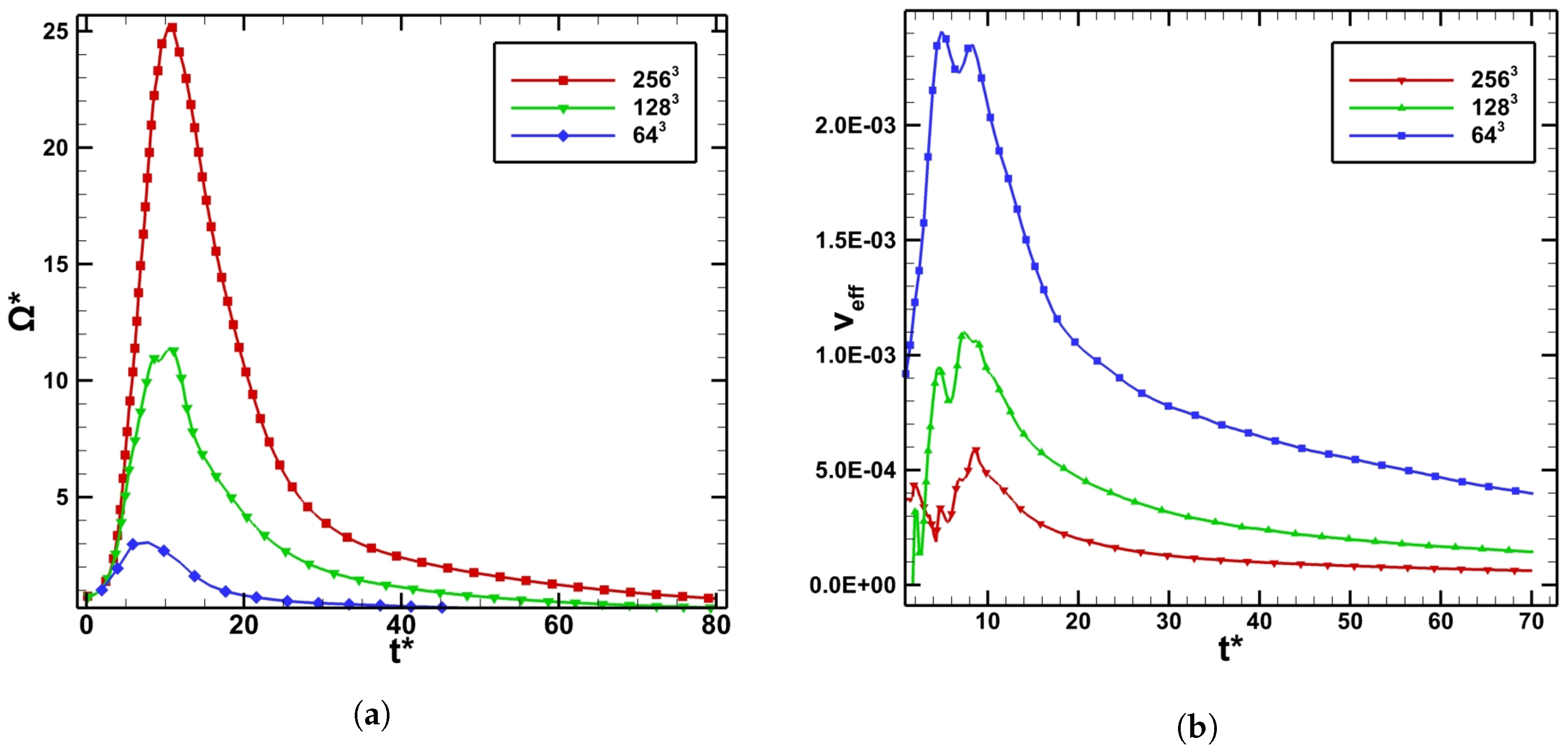
The production of vorticity is monitored for all numerical schemes and all grid levels in terms of enstrophy and effective viscosity. The latter is defined as the ratio between the kinetic energy dissipation rate and enstrophy. Figure 5 shows the evolution of the volume average of enstrophy in time and the related development of the volumetrically-averaged effective viscosity obtained using the LES approach. DSMG-M3 results will be representative of all numerical schemes used within the ILES approach, which showed similar trends. In theory, the enstrophy should grow to infinity for an inviscid flow. Thus, this parameter is very important to study the “effective viscosity” that damps the enstrophy and stops it from growing to infinity in time. The enstrophy could be considered, in conclusion, as one of the criteria that could be used to investigate the performance and resolving power of a numerical scheme. The production of vorticity that could be observed at the early laminar stages is due to the stretching of the Taylor–Green vortex where the large-scale vorticity structures are driven towards the symmetry plane. All the numerical schemes predict a decrease in enstrophy at the stage when the flow becomes under-resolved representing the peak of the kinetic energy dissipation rate. The enstrophy decreases due to the dissipation inherent in the numerical scheme or the dissipation of the subgrid-scale model, which could be considered as an implicit or explicit numerical viscosity that is damping the production of vorticity. Using finer grid resolutions, the effective viscosity decreases, and more enstrophy could be produced. This result seems obvious since the enstrophy and effective viscosity are inversely proportional.
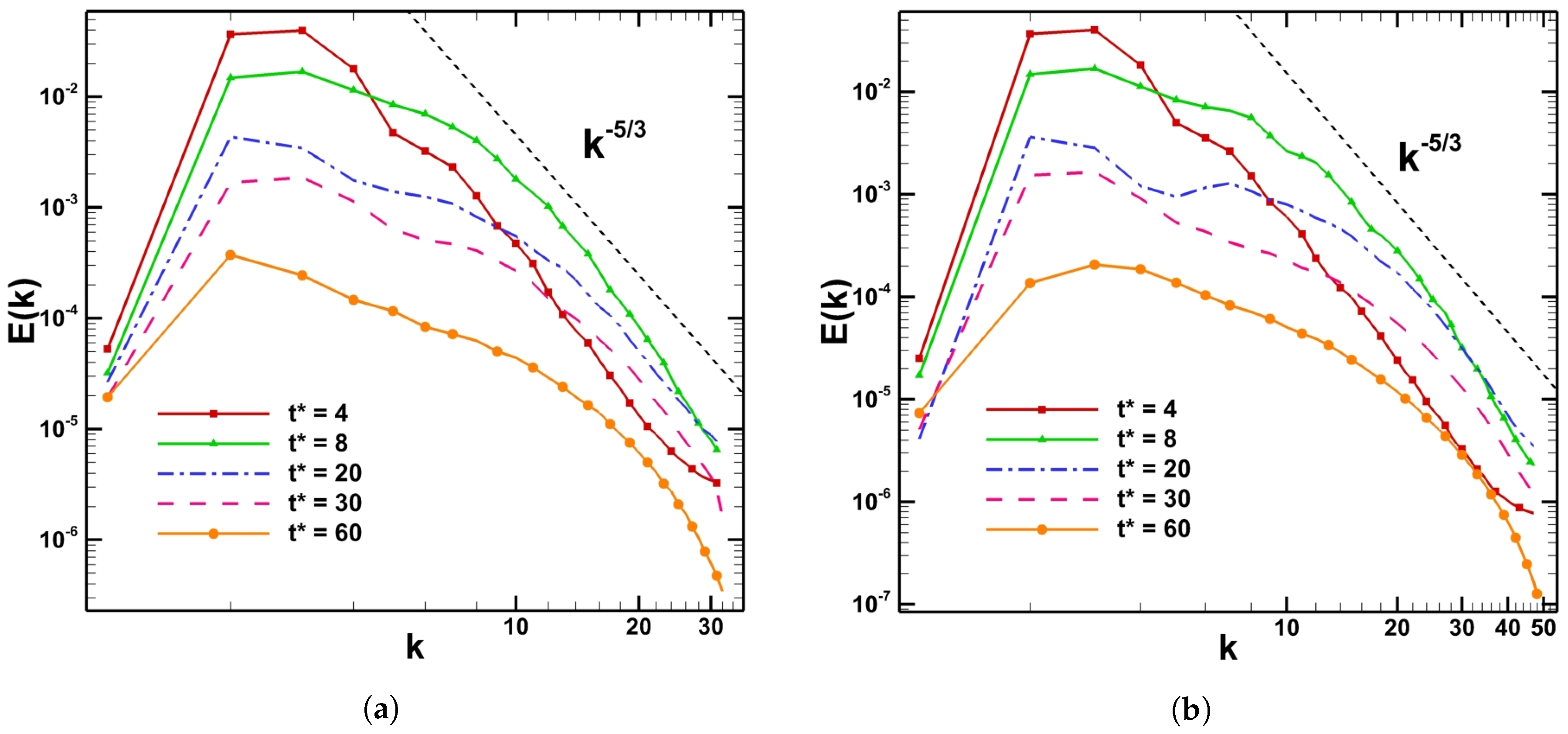
The kinetic energy spectra were monitored for all the numerical methods used in this study. The observation of kinetic energy spectra helps with understanding the flow topology and the energy cascade process. Figure 6 presents the kinetic energy spectra obtained at different times using the M3-KK scheme on 64 and , representing the same behaviour as the other schemes used.
A peak in the kinetic energy spectra could be observed for wavenumbers . The same peak was observed in the study of Drikakis et al. [29], where the authors explain that this peak in the energy spectra represents the imprint of the initial conditions used to initialize the velocity field at . At the very early laminar stage (), all the numerical schemes predicted a spectrum, as has been presented in the DNS study of Brachet et al. and that corresponds to the spectrum usually found for a two-dimensional flow. This result is coherent with the fact that the three-dimensional vortex field of the TGV is initialized by a two-dimensional velocity field, and hence, the two-dimensional character of the flow is explained. As the flow becomes under-resolved, all the numerical methods including the dynamic Smagorinsky subgrid-scale model consistently emulate a spectrum as predicted for the decaying turbulence kinetic energy spectrum. It should be noted that the dissipation of kinetic energy and the exchange of energy between the large and small scales is due to numerical dissipation inherent in the schemes being used, which acts as an implicit subgrid-scale model, and the dissipation of the explicit subgrid-scale model used in LES. The fact that all the methods succeeded in predicting the spectrum indicates that Taylor–Green vortex flow is characterised by an inertial subrange where the small-scale vortices lose kinetic energy at the grid size level due to numerical dissipation. As the mesh is refined, the slope becomes more accurately presented, and one could notice that at very late stages of the flow (), the Kolmogorov scale becomes more established. It should be reminded that at this stage of TGV flow, the small-scale worm-like vortices fade-away, similarly to homogeneously-decaying turbulence.
3.3. Modified Equation Analysis
In this section, the effect of the truncation error of the second-order upwind scheme has been investigated, and the discretization of the convective term of the fully-compressible Navier–Stokes equations is carried out within the framework of the LES approach. The modified equation analysis, applied to the convective term of Navier–Stokes equations, yields the following formulation for the truncation error of the second-order upwind scheme as:
As explained earlier, the truncation error of the numerical scheme is usually neglected by most of the researchers, who claim that it has a minor effect on the accuracy of the solution, and only the numerical dissipation of the subgrid-scale model is considered. Therefore, this section aims to clarify the idea that the truncation error could have a significant contribution to the numerical dissipation of the solution. The Taylor–Green vortex helps with understanding if the subgrid-scale model dissipation is enough to predict the correct amount of kinetic energy dissipation rate or the truncation error is participating in the dissipation of kinetic energy observed during the course of the TGV simulations. For that purpose, LES performed in ANSYS-FLUENT using the dynamic Smagorinsky subgrid-scale model, second-order upwind scheme for spatial discretisation and first-order upwind scheme for temporal discretisation are considered. The truncation error derived on the right-hand side of Equation (15) is computed using a User-Defined Function (UDF) in ANSYS-FLUENT. One could notice that the truncation error of the second-order upwind scheme has second- and third-order partial derivatives in addition to mixed partial derivatives. Only the effect of second-order partial derivatives, which are considered as the leading-order terms, is investigated in this study. It should be reminded that the second-order partial derivatives that exist in the formulation of the truncation error are present due to the fact that a first-order accurate method is used for temporal discretisation. Using higher-order temporal methods would induce third- or higher-order partial derivatives in the equation. Figure 7 represents the time evolution of the leading second-order partial derivatives terms in the truncation error formulation of the second-order upwind scheme, without considering the second-order mixed partial derivatives and compared to the kinetic energy dissipation rate obtained using the dynamic Smagorinsky subgrid-scale model and second-order upwind scheme (DSMG-U2) on a 64 grid. The expression of the computed terms taken from the truncation error in Equation (15) is:
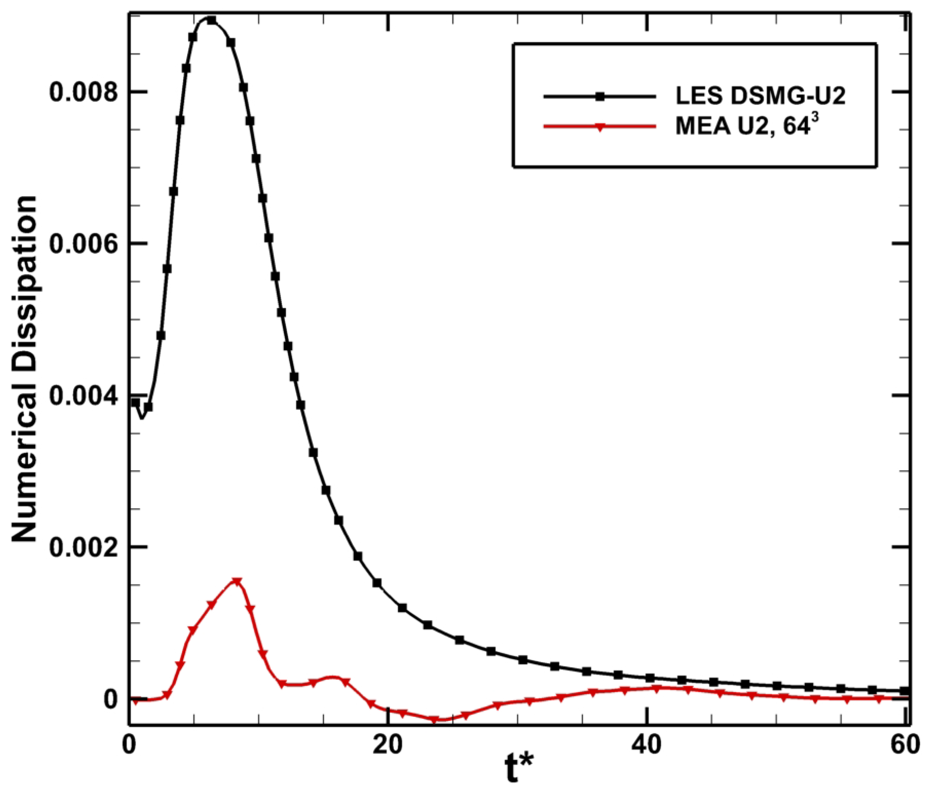
The observed volumetrically-averaged truncation error has a time behaviour similar to the kinetic energy dissipation rate. The trend of the truncation error is characterised by an increase near reaching a peak at about similar to what was predicted by all the numerical schemes and the DNS study of Brachet et al. [20,21]. The truncation error decreases in the stages where the flow becomes disorganized. For , negative values of truncation error could be observed, which could be due to a dispersive behaviour of the scheme since the truncation error is derived on the right-hand side in the modified Equation (16), and hence, the negative values will be added to the left-hand side part, which induces a dispersion of the numerical solution. It is obvious from Figure 7 that the truncation error composed of second-order partial derivatives is not negligible compared to the kinetic energy dissipation rate despite the fact that the values of the discretisation error are significantly small compared to the dissipation of kinetic energy. It should be reminded that the dissipation of kinetic energy is due to the dissipation of the subgrid-scale model and the effect of truncation error of the numerical scheme. Hence, the evolution of the kinetic energy dissipation rate represented in Figure 7 contains both effects of the subgrid-scale model and the truncation error of the second-order upwind scheme. Therefore, if the truncation error is subtracted from the kinetic energy dissipation rate, an estimation of the subgrid-scale model dissipation could be obtained, as will be shown in Figure 8.
The DSMG model is under-predicting the kinetic energy dissipation since its peak of dissipation is lower than the one predicted by the total dissipation of kinetic energy considering the truncation error of the upwind scheme, as well. At , dispersion in the trend of DSMG dissipation is observed due to the negative values of truncation error representing the dispersive behaviour of the scheme. the conclusion that could be drawn is that the truncation error of the numerical scheme could play a significant role in the dissipation of kinetic energy which is added to the subgrid scale model dissipation that is not giving the correct amount of numerical dissipation to model the small scales on its own. That gives motivation for researchers to reconsider their idea of always neglecting the dissipation error that is yielded by the numerical scheme being used.
4. Conclusions
All the numerical methods predicted a decrease in kinetic energy during the course of the simulations performed. The decay is due to the numerical dissipation embedded in the numerical schemes used for ILES and to the dissipation of the subgrid-scale model when classical LES is used. The numerical dissipation of the scheme is beneficial as long as it is lower than the physical dissipation; otherwise, the dissipation could overwhelm the accuracy of the solution. It has been found that increasing the accuracy of the numerical method prolongs the conservation of kinetic energy in time. In effect, the resolving power of the second-order MUSCL scheme with the Van Albada slope limiter was the least among all other numerical schemes. That was expected, since the latter is a second-order method, whereas the other methods have third-order accuracy. In addition to that, the effective viscosity decreases when the mesh is refined and more enstrophy is produced. The conclusion is that the numerical dissipation decreases and more vorticity is produced with finer grid resolutions, which was expected since higher gradients could be handled with finer grids, and hence, the accuracy increases. Nevertheless, all the schemes showed a non-physical behaviour with the mesh characterised by an increase in the kinetic energy dissipation at , when the flow becomes disorganized. This behaviour vanishes on finer grids, and that decrease in kinetic energy dissipation was not observed in LES since the grid was not adopted for the classical LES study. Furthermore, finer grid resolutions corresponded to higher Reynolds number trends compared to DNS data from Brachet et al. [20,21]. Thus, the explicit and implicit subgrid-scale viscosities predict a Re-independent limit when refining the grid resolution, where the peak of kinetic energy dissipation will be the same. The decay exponent falls in the range of the theoretical value predicted in [33] as far as the mesh is refined. The onset of decay showed that M2-VA starts loosing kinetic energy first, then M3-DD, and the least dissipative is the M3-KK scheme. LES results showed that the dissipation of kinetic energy starts earlier than the one predicted by all the schemes used within the framework of ILES on the same grid size. Nonetheless, the kinetic energy starts to decay later when the mesh is refined. Finally, the kinetic energy spectrum was monitored for all schemes and all grid levels in the study of TGV dynamics. A peak in the kinetic energy spectra is present at small wavenumbers, representing the effect of initial conditions used at . All the numerical schemes predicted the spectrum at ; the same was pointed out in the study of Brachet et al. [20,21], representing the spectra that are usually observed for two-dimensional turbulence. When the flow becomes under-resolved, all numerical methods succeeded in predicting a spectrum, which induces that the Taylor–Green vortex is characterised by an inertial subrange where the kinetic energy dissipates into heat due to numerical dissipation either from the numerical scheme or from the subgrid-scale model.
The analytical formulation of the truncation error of the second-order upwind scheme obtained using the modified equations analysis was investigated. The effect of second-order partial derivatives was examined without considering the influence of mixed derivatives. The study showed that second-order partial derivatives induce a truncation error that is not negligible compared to the total dissipation of kinetic energy. It should be reminded that the kinetic energy dissipation rate contains both the subgrid-scale model and truncation error effects. If the discretisation error is subtracted from the total kinetic energy dissipation, the obtained estimate of the subgrid-scale model dissipation underpredicts the correct amount of kinetic energy dissipation. For , negative values of truncation error were observed inducing a dispersive behaviour of the numerical scheme, since the negative values will be added to the solution, which is dispersed.
As a conclusion, the leading-order terms of the truncation error induce a significant dissipation that could not be neglected, as many times done in practice.
Acknowledgments
The present research work was financially supported by the Centre for Computational Engineering Sciences at Cranfield University under Project Code EEB6001R. The authors would like to acknowledge the IT support and the use of the High Performance Computing (HPC) facilities at Cranfield University, U.K. We would like to acknowledge the constructive comments of the reviewers of the Aerospace journal.
Author Contributions
Moutassem El Rafei, László Könözsy, and Zeeshan Rana contributed equally to this paper.
Conflicts of Interest
The authors declare no conflict of interest.
Abbreviations
The following abbreviations are used in this manuscript:
| CFL | Courant–Friedrichs–Lewy number |
| DNS | Direct Numerical Simulation |
| DSMG | Dynamic Smagorinsky model |
| FFT | Fast Fourier Transform |
| HLLC | Harten–Lax–van Leer–Contact Riemann solver |
| ILES | Implicit Large Eddy Simulation |
| LES | Large Eddy Simulation |
| MEA | Modified Equation Analysis |
| M2-VA | Second-order MUSCL scheme with Van Albada slope limiter |
| M3-DD | Third-order MUSCL scheme with the Drikakis and Zoltak limiter |
| M3-KK | Third-order MUSCL scheme with the Kim and Kim slope limiter |
| MUSCL | Monotonic Upwind Scheme for Conservation Laws |
| PDE | Partial Differential Equation |
| RANS | Reynolds Averaged Navier–Stokes |
| SGS | Smagorinsky Subgrid-Scale model |
| TGV | Taylor–Green Vortex |
References
- Boris, J.P. On large eddy simulation using subgrid subgrid turbulence models. In Whither Turbulence? Turbulence at the Crossroads. Lecture Notes in Physics; Lumley, J.L., Ed.; Springer: Berlin/Heidelberg, Germany, 1990; pp. 344–353. [Google Scholar]
- Grinstrein, F.F.; Margolin, L.G.; Rider, W.J. Implicit Large Eddy Simulation—Computing Turbulent Fluid Dynamics; Cambridge University Press: New York, NY, USA, 2007. [Google Scholar]
- Dairy, T.; Lamballais, E.; Laizet, S.; Vassilicos, J.C. Numerical dissipation vs. subgrid scale modelling for large eddy simulation. J. Comput. Phys. 2017, 337, 252–274. [Google Scholar] [CrossRef]
- Garnier, E.; Adams, N.; Sagaut, P. Large Eddy Simulation for Compressible Flows; Springer: Dordrecht, The Netherlands, 2009. [Google Scholar]
- Chow, F.K.; Moin, P.A. Further study of numerical errors in large-eddy simulations. J. Comput. Phys. 2003, 184, 366–380. [Google Scholar] [CrossRef]
- Vreman, A.W.; Sandham, N.D.; Luo, K.H. Compressible mixing layer growth and turbulence characteristics. J. Fluid Mech. 1996, 320, 235–258. [Google Scholar] [CrossRef]
- Garnier, E.; Mossi, M.; Sagaut, P.; Comte, P.; Deville, M. On the use of shockcapturing schemes for large-eddy simualtion. J. Comput. Phys. 1999, 153, 273–311. [Google Scholar] [CrossRef]
- Domaradzki, J.A.; Xiao, Z.; Smolarkiewicz, P.K. Effective eddy viscosities in implicit large eddy simulations of turbulent flows. Phys. Fluids 2003, 15, 1890–3893. [Google Scholar] [CrossRef]
- Bonelli, F.; Viggiano, A.; Magi, V. How does a high density ratio affect the near- and intermediate-field of high-Re hydrogen jets. Int. J. Hydrog. Energy 2016, 41, 15007–15025. [Google Scholar] [CrossRef]
- Cook, A.W. Artificial fluid properties for Large-Eddy Simulation of compressible turbulent mixing. Phys. Fluids 2007, 19, 055103. [Google Scholar] [CrossRef]
- Kawai, S.; Lele, S.K. Large-Eddy Simulation of jet mixing in supersonic cross-flows. AIAA J. 2010, 48, 2063–2083. [Google Scholar] [CrossRef]
- De Wiart, C.C.; Hillewaert, K.; Bricteux, L.; Winckelmans, G. Implicit LES of free and wall-bounded turbulent flows based on the discontinuous Galerkin/symmetric interior penalty method. Int. J. Numer. Meth. Fluids 2015, 78, 335–354. [Google Scholar] [CrossRef]
- Aspden, A.; Nikiforakis, N.; Dalziel, S.; Bell, J. Analysis of implicit LES methods. Commun. Appl. Math. Comput. Sci. 2008, 3, 103–126. [Google Scholar] [CrossRef] [Green Version]
- Könözsy, L. Multiphysics CFD Modelling of Incompressible Flows at Low and Moderate Reynolds Numbers. Ph.D. Thesis, Cranfield University, Cranfield, UK, 2012. [Google Scholar]
- Tsoutsanis, P.; Kokkinakis, I.W.; Könözsy, L.; Drikakis, D.; Williams, R.J.R.; Youngs, D.L. Comparison of structured- and unstructured-grid, compressible and incompressible methods using the vortex pairing problem. Comput. Methods Appl. Mech. Eng. 2015, 293, 207–231. [Google Scholar] [CrossRef] [Green Version]
- Könözsy, L.; Drikakis, D. A unified fractional-step, artificial compressibility and pressure-projection formulation for solving the incompressible Navier–Stokes equations. Commun. Comput. Phys. 2014, 16, 1135–1180. [Google Scholar] [CrossRef]
- Rana, Z.A.; Thornber, B.; Drikakis, D. Dynamics of Sonic Hydrogen Jet Injection and Mixing Inside Scramjet Combustor. Eng. Appl. Comput. Fluid Mech. 2013, 7, 13–39. [Google Scholar] [CrossRef]
- Sakellariou, K.; Rana, Z.A.; Jenkins, K.W. Optimisation of the surfboard fin shape using computational fluid dynamics and genetic algorithms. Proc. Inst. Mech. Eng. Part P J. Sports Eng. Technol. 2017, 231, 344–354. [Google Scholar] [CrossRef]
- Fletcher, C.A.J. Computational Techniques for Fluid Dynamics 1, 2nd ed.; Springer: Berlin, Germany, 1990. [Google Scholar]
- Brachet, M.E. Direct simulation of three-dimensional turbulence in the taylor-green vortex. Fluid Dyn. Res. 1991, 8, 1–8. [Google Scholar] [CrossRef]
- Brachet, M.E.; Meiron, D.I.; Orszag, A.; Nickel, B.G.; Morf, R.H.; Frisch, U. Small-scale structure of the taylor-green vortex. J. Fluid Mech. 1983, 130, 411–452. [Google Scholar] [CrossRef]
- Spiteriand, R.J.; Ruuth, S.J. A new class of optimal high-order strong-stability-preserving time discretization method. SIAM J. Numer. Anal. 2002, 40, 469–491. [Google Scholar] [CrossRef]
- Drikakis, D.; Hahn, M.; Mosedale, A.; Thornber, B. Large eddy simulation using high-resolution and high-order methods. Philos. Trans. R. Soc. A 2009, 367, 2985–2997. [Google Scholar] [CrossRef] [PubMed] [Green Version]
- Kim, K.H.; Kim, C. Accurate, efficient and monotonic numerical methods for multi-dimensional compressible flows. Part II: Multi-Dimensional limiting process. J. Comput. Phys. 2005, 208, 570–615. [Google Scholar] [CrossRef]
- Zoltak, J.; Drikakis, D. Hybrid upwind methods for the simulation of unsteady shock-wave diffraction over a cylinder. Comput. Methods Appl. Mech. Eng. 1998, 162, 165–185. [Google Scholar] [CrossRef]
- Hahn, M. Implicit Large-Eddy Simulation of Low-Speed Separated Flows Using High-Resolution Methods. Ph.D. Thesis, Fluid Mechanics and Computational Science, Cranfield University, Cranfield, UK, 2008. [Google Scholar]
- Tennekes, H.; Lumley, J.L. A First Course in Turbulence; The MIT Press: Cambridge, MA, USA, 1972. [Google Scholar]
- Kolmogorov, A.N. The local structure of turbulence in incompressible viscous fluid for very large Reynolds number. Proc. USSR Acad. Sci. 1941, 30, 301–305. [Google Scholar] [CrossRef]
- Drikakis, D.; Fureby, C.; Grinstein, F.; Youngs, D. Simulation of transition and turbulence decay in the Taylor–Green vortex. J. Turbul. 2007, 8, 1–12. [Google Scholar] [CrossRef]
- Fauconnier, D.; Langhe, C.D.; Dick, E. Construction of explicit and implicit dynamic finite difference schemes and application to the large-eddy simulation of the Taylor–Green vortex. J. Comput. Phys. 2009, 228, 8053–8084. [Google Scholar] [CrossRef]
- Fauconnier, D.; Bogey, C.; Dick, E. On the performance of relaxation filtering for large-eddy simulation. J. Turbul. 2013, 14, 22–49. [Google Scholar] [CrossRef]
- Zhou, Y.; Grinstein, F.F.; Wachtor, A.J.; Haines, B.M. Estimating the effective Reynolds number in implicit large-eddy simulation. Phys. Rev. E 2014, 89, 013303. [Google Scholar] [CrossRef] [PubMed]
- Skrbek, L.; Stalp, S.R. On the decay of homogeneous isotropic turbulence. Phys. Fluids 2000, 12, 1997–2019. [Google Scholar] [CrossRef]
Figure 1.
Geometry of the outer computational domain.

Figure 2.
The Taylor–Green Vortex (TGV) flow using isosurfaces of Q-criterion = 0 coloured with the dimensionless kinetic energy obtained through the third-order MUSCL scheme with the Kim and Kim slope limiter (M3-KK) on a grid. (a) t* = 0; (b) t* = 4; (c) t* = 8; (d) t* = 20; (e) t* = 30; (f) t* = 60.

Figure 3.
Evolution of the volumetrically-averaged kinetic energy represented in logarithmic scale and kinetic energy dissipation obtained on , and grids for the ILES approach and , and for the LES approach. (a) ILES, (); (b) ILES, (); (c) ILES, (); (d) ILES, (); (e) ILES, (); (f) ILES, (); (g) LES, ; (h) LES, .


Figure 4.
Evolution of the volumetrically-averaged kinetic energy dissipation obtained on all the grid levels and compared to DNS data of Brachet et al. [20,21]. (a) ILES, M3-KK; (b) LES, DSMG-M3.

Figure 5.
Variation of the volume-averaged enstrophy and the volume-averaged effective viscosity during the course of the simulations performed using DSMG-M3 on three different grid levels. (a) LES, enstrophy; (b) LES, effective viscosity.
Figure 5.
Variation of the volume-averaged enstrophy and the volume-averaged effective viscosity during the course of the simulations performed using DSMG-M3 on three different grid levels. (a) LES, enstrophy; (b) LES, effective viscosity.

Figure 6.
Kinetic energy spectra obtained using the MUSCL scheme with M3-KK slope limiter on and grids. (a) ILES, M3-KK ( mesh); (b) ILES, M3-KK ( mesh).
Figure 6.
Kinetic energy spectra obtained using the MUSCL scheme with M3-KK slope limiter on and grids. (a) ILES, M3-KK ( mesh); (b) ILES, M3-KK ( mesh).

Figure 7.
Contribution of second-order partial derivatives in the truncation error of the second-order upwind scheme obtained using Modified Equation Analysis (MEA) on a 64 mesh and compared to the kinetic energy dissipation rate obtained using DSMG-U2 on the same grid.
Figure 7.
Contribution of second-order partial derivatives in the truncation error of the second-order upwind scheme obtained using Modified Equation Analysis (MEA) on a 64 mesh and compared to the kinetic energy dissipation rate obtained using DSMG-U2 on the same grid.

Figure 8.
Dissipation of the DSMG model obtained by subtracting the truncation error of the second-order upwind scheme (MEA U2) from the total kinetic energy dissipation rate obtained on a grid.
Figure 8.
Dissipation of the DSMG model obtained by subtracting the truncation error of the second-order upwind scheme (MEA U2) from the total kinetic energy dissipation rate obtained on a grid.


Table 1.
Decay exponent and onset of kinetic energy decay obtained using high-order non-oscillatory finite volume numerical schemes.
Table 1.
Decay exponent and onset of kinetic energy decay obtained using high-order non-oscillatory finite volume numerical schemes.
| Grid | |||||||||
|---|---|---|---|---|---|---|---|---|---|
| Scheme | M2-VA | M3-KK | M3-DD | M2-VA | M3-KK | M3-DD | M2-VA | M3-KK | M3-DD |
| Decay Exponent P | 1.594 | 1.843 | 1.506 | 1.91 | 2.183 | 2.083 | 2.083 | 2.197 | 2.065 |
| Onset of Decay | 1.75 | 2.015 | 1.845 | 2.375 | 2.711 | 2.618 | 2.908 | 3.172 | 3.026 |
Table 2.
Decay exponent and onset of kinetic energy decay obtained using the dynamic Smagorinsky subgrid-scale model with the MUSCL third-order scheme.
Table 2.
Decay exponent and onset of kinetic energy decay obtained using the dynamic Smagorinsky subgrid-scale model with the MUSCL third-order scheme.
| Scheme | DSMG-M3 | ||
|---|---|---|---|
| Grid | |||
| Decay Exponent P | 1.588 | 1.975 | 1.989 |
| Onset of Decay | 1.066 | 1.875 | 4.296 |
© 2017 by the authors. Licensee MDPI, Basel, Switzerland. This article is an open access article distributed under the terms and conditions of the Creative Commons Attribution (CC BY) license (http://creativecommons.org/licenses/by/4.0/).
Share and Cite
MDPI and ACS Style
El Rafei, M.; Könözsy, L.; Rana, Z. Investigation of Numerical Dissipation in Classical and Implicit Large Eddy Simulations. Aerospace 2017, 4, 59. https://0-doi-org.brum.beds.ac.uk/10.3390/aerospace4040059
AMA Style
El Rafei M, Könözsy L, Rana Z. Investigation of Numerical Dissipation in Classical and Implicit Large Eddy Simulations. Aerospace. 2017; 4(4):59. https://0-doi-org.brum.beds.ac.uk/10.3390/aerospace4040059
Chicago/Turabian StyleEl Rafei, Moutassem, László Könözsy, and Zeeshan Rana. 2017. "Investigation of Numerical Dissipation in Classical and Implicit Large Eddy Simulations" Aerospace 4, no. 4: 59. https://0-doi-org.brum.beds.ac.uk/10.3390/aerospace4040059
Note that from the first issue of 2016, this journal uses article numbers instead of page numbers. See further details here.