1. Introduction
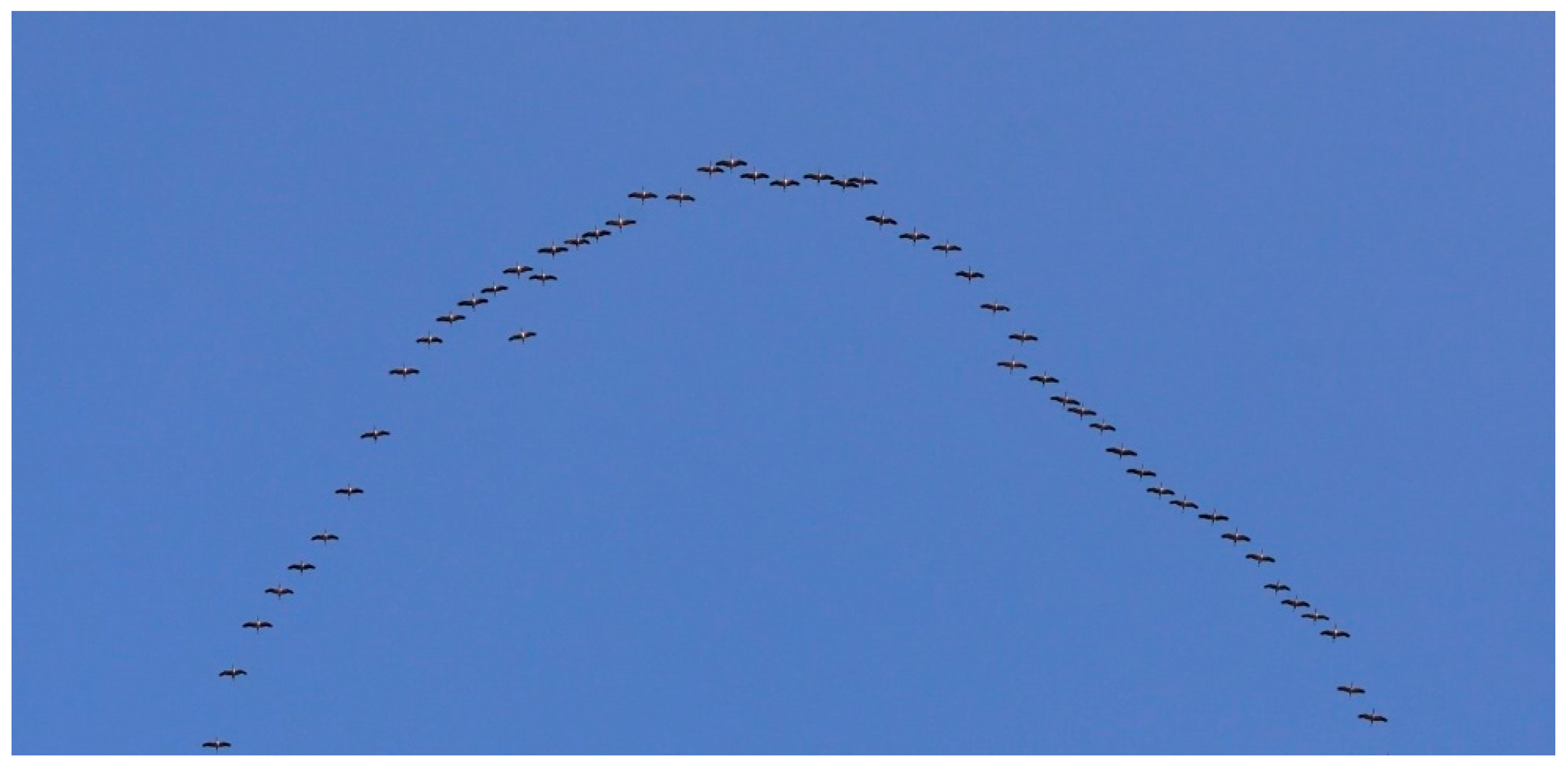
The principle of formation flight as it can be observed with migratory birds (see
Figure 1) has been known for over a century and Wieselsberger [
1] was the first to describe the underlying principle. In contrast to other flocks of birds that mainly serve the purpose of self-protection against predators or other purposes such as navigational advantages, some migratory birds use this technique to tap an external source of energy as it is given by another bird’s wake vortex in order to save energy and to extend their range during migration [
2]. In principle, during formation flight the following birds position themselves in the wake vortices of the preceding birds literally surfing on the upwash of the wake and, therefore, using less energy for flight. If the preceding birds get weaker after some time, they fall back, and the leading positions are swapped with the followers.
This aerodynamic effect can be transferred to man-made aircraft and is nowadays also called aerodynamic formation flight or aircraft wake-surfing for efficiency (AWSE). As with the migratory birds, the thrust of an aircraft flying in the upwash of another aircraft’s wake can be reduced.
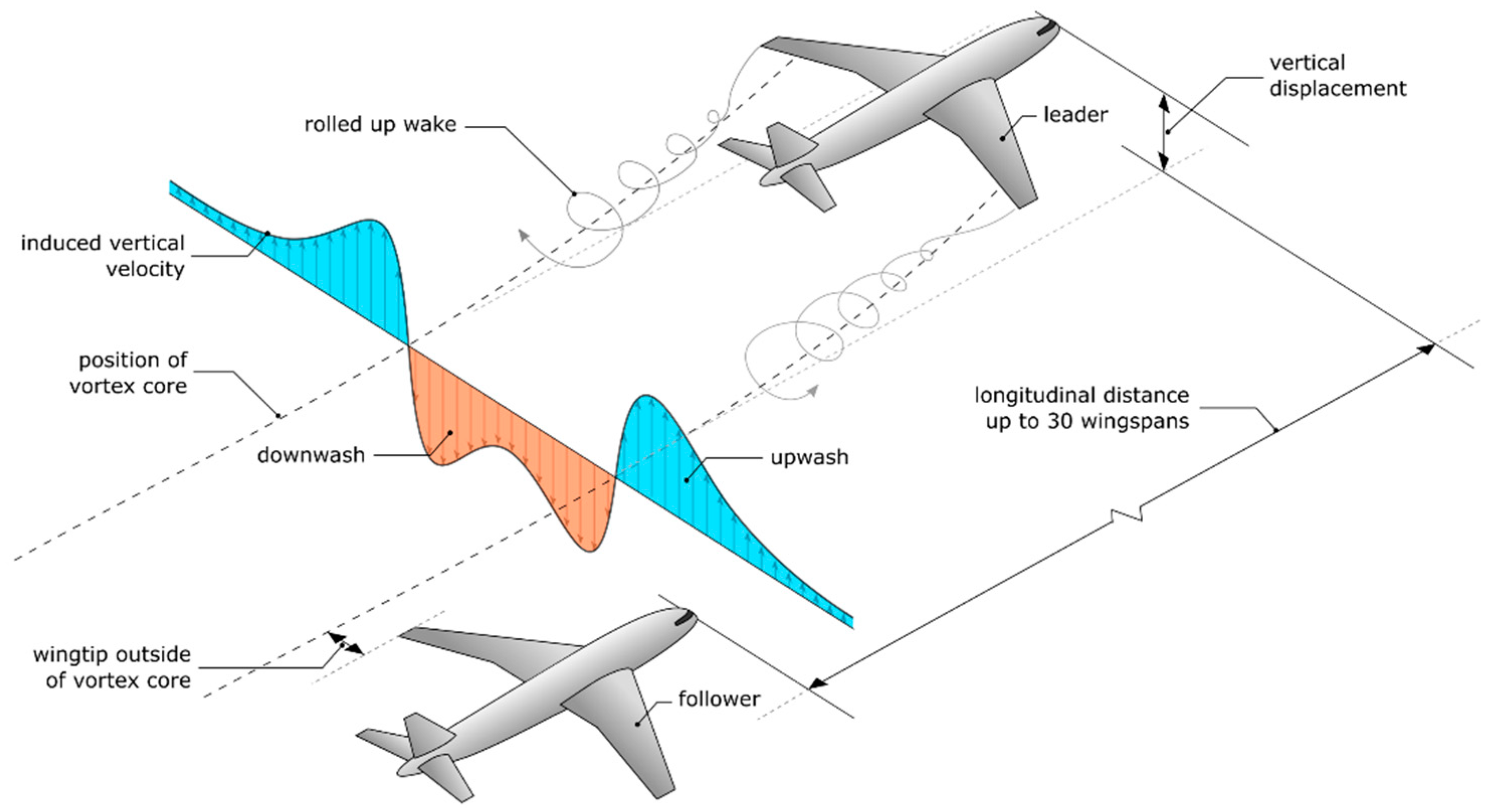
Figure 2 shows the basic configuration of a two-aircraft formation performing AWSE as modeled within this work. The follower aircraft is assumed to position itself about 30 wingspans behind the leader (extended formation flight; EFF) in the stable part of the wake vortex of the leader. To avoid buffeting and to maintain a stable flight state the follower is assumed to be positioned in the upwash field created by the leaders wake vortex with its wingtip at about 5% of the wingspan outside of the vortex core.
As by self-induction the wake vortex descends behind the leader, the follower needs to fly lower. However, as the follower positions itself in relation to the wake vortex of the leader and not to the leader itself the vertical displacement is not considered in this work.
While conducting AWSE the follower finds itself in an uprising air mass and would increase its altitude if not compensated for. This can be achieved by introducing a descent in relation to the surrounding air mass. As a result, the thrust setting needs to be reduced in order to maintain a stable flight state [
3]. The thereby harvested energy can then be traded for longer flight time, larger range or less fuel consumption, the latter leading to cost savings or higher payloads accordingly [
4]. These prospects make AWSE interesting for aviation and since the first description of the basic principle, research has been conducted on the various aspects of this new procedure to adapt it to man-made aircraft. Beside research in aerodynamics, aircraft design and control theory, flight testing (e.g., [
5,
6,
7,
8]) showed that the new procedure can be successfully executed by aircraft and that a considerable reduction of the fuel flow of the follower aircraft can be achieved in practice. To introduce this new procedure for a wider range of flights, operational aspects have to be considered in addition to the flight testing. Several works focused on the estimation of optimal joint flight tracks for formations (e.g., [
9,
10,
11]) as well as on the prediction of the achievable fuel saving benefits on system level based on real world flight plan data (e.g., [
12,
13,
14,
15]). For an exemplary fleet of aircraft, the estimated values for the relative fuel saving benefit were found to be within the range of 3–5%. Other research areas connected with formation flight include regulations (e.g., [
16]) as well as flight planning [
17] and more.
In the context of anthropogenic climate change, a new facet of aerodynamic formation flight appears as the reduced fuel consumption also yields a reduction of the emission of greenhouse gases (or precursors). Introducing a novel approach, we present for the first time an analysis of the potential climate impact reduction due to AWSE on a fleet level, by identifying formations based on global flight plan data. Within our approach several aspects are considered such as routing, aerodynamic modeling as well as the climate impact of CO
2 and especially non-CO
2 effects, arising from contrail-cirrus, NO
x- and H
2O-emissions. The non-CO
2 effects are particularly important, considering that location and quantity of the emissions caused by a formation can change due to the adapted routing. Furthermore, saturation effects of both contrail formation and ozone formation occur in the cumulated wake of a formation [
18,
19].
2. Approach and Methods
2.1. General Approach
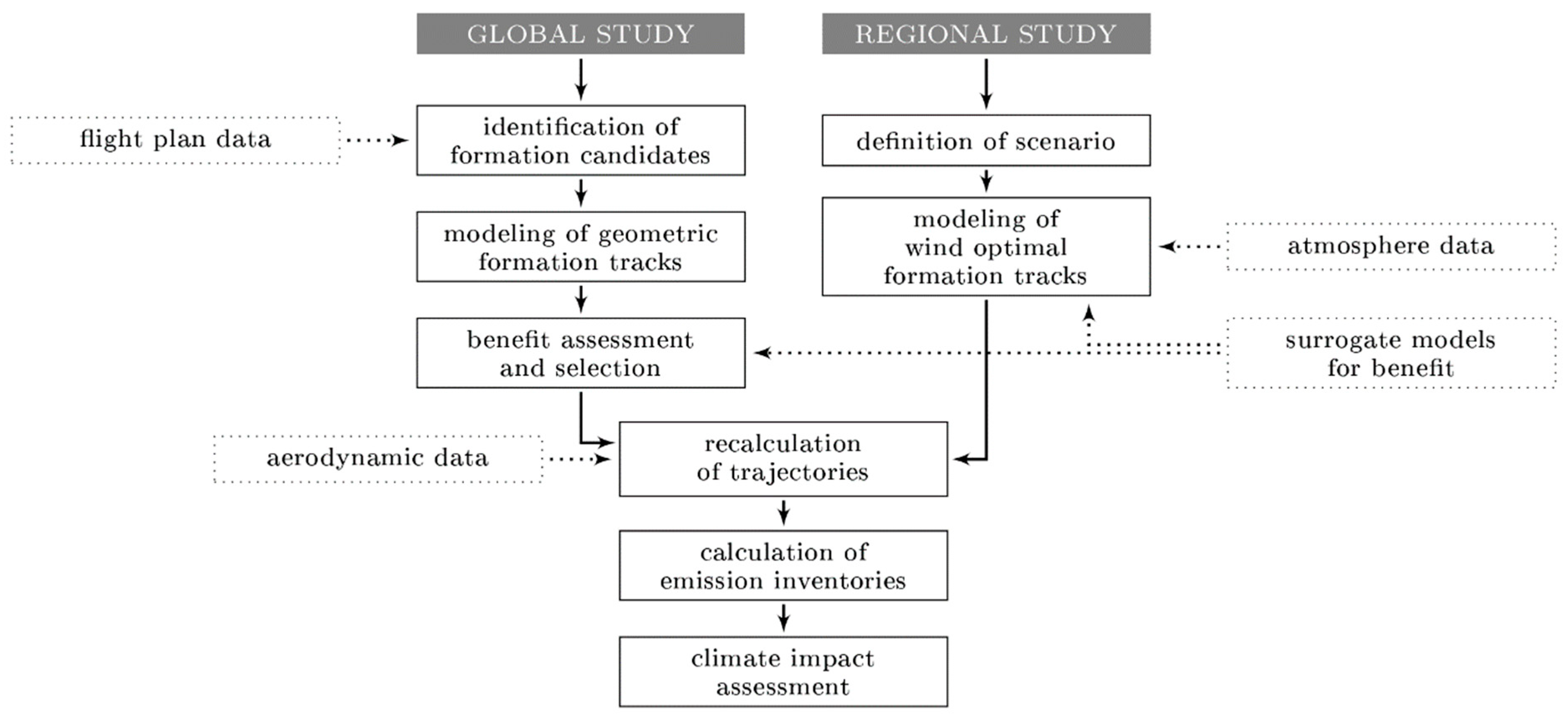
In order to quantify the climate impact mitigation potential of AWSE, this paper presents an interdisciplinary approach combining the fields of aerodynamics, aircraft operations and atmospheric physics in an integrated model chain. The approach we followed in the study is depicted in
Figure 3. It shows the two main studies that we conducted in order to assess the climate impact of AWSE as two branches with a global study (left branch) in contrast to a regional study focusing on the North Atlantic flight corridor (right branch). In the latter wind effects were considered additionally for optimization of the formation routing. Both studies are generally based on two-aircraft formations, assuming both aircraft to maintain a stable AWSE formation during cruise flight, constituting a single beneficial segment. However, possible maneuvers such as positional changes, breakups or rejoins are not considered. Furthermore, we assumed that the formation maintains a fixed altitude (formation cruise altitude; FCA) as well as a fixed speed (formation cruise Mach number; FCM) while conducting AWSE. In the following, the two studies are briefly described, followed by a detailed description of the applied methodology used for the single steps.
2.2. Global Study
In the global study, representative formation scenarios are derived for the world’s major airports by an assessment of global flight plans. Due to the huge amount of possible two-aircraft combinations between the single flights, the formation candidates are initially filtered in order to exclude all impractical formations. All remaining formation candidates are subsequently modeled and evaluated using surrogate models that can predict the AWSE benefits based on the formation route geometry (FRG) and the general mission data. Based on this assessment, the formation candidates with the highest relative benefit are selected to constitute a formation flight plan. The formations contained in this formation flight plan are subsequently recalculated by applying an adapted trajectory calculation tool. In our approach we use databases to assess the aerodynamic interactions between the formation members during the trajectory calculation to estimate the changed fuel flow of the follower. The trajectories are then used to derive emission inventories for the scenario under evaluation. Based on these inventories, the climate impact is then quantitatively estimated using the average temperature response (ATR) as climate metric, calculated as an average global near surface temperature change over a time horizon of 50 years using an adapted version of the climate model AirClim [
20] accounting for the saturation effects in the cumulated wake of the formation [
18].
2.3. Regional Study
In the regional study, a special focus is set on the North Atlantic (NAT). Since wind has been shown to bear a strong effect on the optimal routing and the achievable benefits [
21] as well as on the optimal timing [
22] of a formation, these effects are additionally considered in the regional study. For a predefined set of double origin–destination pairs (DODP), wind optimized formation- and reference routes are estimated. These routes are then used to assess the climate impact by detailed recalculation, creation of emission inventories and climate assessment as in the global study described above. Although the regional study does not represent formations derived from actual flight plans, it can be used to assess the climate effect of formation flight in more detail, since the distribution of emissions can be assumed to be closer to reality.
2.4. Methodology
The methods used for the global and regional studies comprise the identification of formation candidates, route modelling and optimization, surrogate modelling of benefits, trajectory calculation, aerodynamic modeling, climate impact modeling and more as shown in
Figure 3. All these methods are briefly presented in the following.
2.4.1. Identification of Formation Candidates
For the global study, an identification of formation candidates is performed using flight plan data extracted from the Sabre AirVision Market Intelligence Database (Sabre-MI). In order to reduce the enormous amount of possible formation pairings, several filters reduce the viable options based on flight time, location of origin and destination airports, range and the direction of the particular flight tracks (see [
23]). Further filters can be set for aircraft types, carrier, airports, and more. The filter settings for the global study assessed in this paper can be found in
Section 3.1.1.
2.4.2. Geometric Modeling of Formation Routes
In a second step, the formation candidates identified during the previously described process are modeled by a geometric approach as presented by Kent and Richards [
11]. Based on the geographically optimized locations of the rendezvous (rendezvous start point; RSP) and separation point (separation end point; SEP), as well as the origins and destinations of the formation members, full formation route geometries (FRGs) are constructed constituting great circle segments between the given points.
Figure 4 shows a schematic view of the general construction of such a FRG as assumed within this work. Each FRG is set up by seven segments: approach (index a), continuation (index c) and reference (index ref) for both leader (index ld) and follower (index fw), as well as their common beneficial segment (index b). The approach, beneficial and continuation segments constitute the AWSE mission (index awse) in contrast to the reference mission of a formation member which is considered in the global study to be the direct great circle connection between origin and destination.
However, if the departure time constraints given by the flight plan are considered, the geometrically optimal rendezvous location (RSP
geo) might not be reachable by the formation members simultaneously. Therefore, the geographically closest applicable rendezvous location (RSP
opt), that fulfills the given timing constraint, is modeled according to Drews et al. [
23].
Figure 4 shows the schematic adaption of an FRG to these constraints (orange, dashed). The rendezvous line (green) marks all possible locations of rendezvous points for the considered formation pairing. The optimal rendezvous location RSP
opt is assumed to be located as close as possible to the geometrically optimal rendezvous location RSP
geo.
2.4.3. Benefit Assessment by Surrogate Models
The benefit estimation for an AWSE formation is based on surrogate models, estimating the relative AWSE efficiency metric
for the whole formation (index f). This metric represents the difference between the burned fuel mass for the reference mission
and the burned fuel mass for the AWSE mission
set into relation of to the burned fuel mass of the reference mission
and aggregated for both formation members (see Equation (1)). Here,
represents the absolute fuel savings of the formation and is additionally used as the absolute formation efficiency metric during the evaluation.
In general, each FRG can be described by the detours
and relative lengths of the different segments
as given by Equations (2) and (3) for both leader (index ld) and follower (index fw). Here,
depicts the length of the air distance of a segment or full track, corresponding to the ground distance in the windless case.
Together with the mission parameters (passenger load factors,
; FCA; FCM) and a scaling length (formation route length of the leader,
), a full formation mission can be described using 11 parameters [
24].
The absolute and relative formation metric can then be estimated by the surrogate models using these parameters according to Equation (4).
To create the corresponding surrogate models, the Kriging method is applied on a set of sample data constituting various FRGs and mission settings selected by design of experiments (DOE) methods. Here, sample plans for model creation and validation are derived for all parameters by Latin hypercube sampling (LHS). The benefits for the sample and validation data are then calculated using the trajectory calculation and aerodynamic modelling as described in the next section. The surrogate models are then created and validated by using the calculation results accordingly. A detailed description of the process of surrogate modelling of formation flight benefits is presented in [
24].
2.4.4. Trajectory Calculation and Aerodynamic Modelling
For the recalculation of the trajectories, an adapted version of the trajectory calculation module (TCM) is applied, which calculates 4D aircraft trajectories using the total-energy model for solving the flight mechanical equations of motion in combination with aircraft performance data, Base of Aircraft Data (BADA 4.2) from EUROCONTROL [
25,
26].
Within this work the aerodynamic modeling according to
Figure 2 is assumed. Here the follower positions itself in the stable part of the wake vortex of the leader at about 30 wingspans behind and with the wingtip 5% of the wingspan outside of the vortex core. As the strength of the wake vortex of the leader depends on its flight state and weight, in the AWSE case the leader’s trajectory is handed over to the follower during the calculation process and the vortex strength is accounted for in the calculation of the reduced fuel flow of the follower. The follower’s benefits for the current flight state are derived from a database of precalculated drag values for the AWSE condition (drag reduction database, DRD) and solo flight (base drag database; BDD). During the trajectory calculation these benefits for the current flight state are obtained from the databases depending on the leader’s and follower’s masses, altitude, speed and the follower’s position in the vortex. The process to set up the corresponding databases using the Athena Vortex Lattice (AVL) method is described in [
27]. A comparison of the AVL method to an analytical model and the approach used in this paper is presented in [
28].
Additionally, wind effects can be accounted for in the course of the trajectory calculation process depending on the scenario under evaluation using European Centre for Medium-Range Weather Forecasts (ECMWF) wind data. As the TCM is optimizing the trajectories in terms of fuel consumption, fuel-for-fuel effects are included in the calculated block fuel masses of the formation members.
2.4.5. Wind Optimal Modeling of Formation Routes
Not only are the AWSE benefits of a formation influenced by wind, but the optimal FRG is also affected. For the estimation of wind optimal formation and reference tracks in the regional study an optimal control approach was developed as presented in [
21]. Here, for each segment of an FRG a wind optimal track is calculated using an optimal control approach. In order to build up a full FRG, all segments of a formation are calculated separately are finally connected. The resulting FRG is subsequently assessed using the surrogate models as described in
Section 2.4.3. This is possible as the surrogate models use the formation route length of the leader (
) for scaling the benefits. In the wind affected case
is given by the air distance in contrast to the windless case where
corresponds to the ground distance. As the geographic locations of the rendezvous (RSP) and separation points (SEP) are variable, they are subject to optimization. Therefore, to find the wind optimal geographic locations of these points, a higher-level pattern search algorithm is used varying both locations simultaneously, pinpointing the combination with maximum benefit. As it is assumed that the AWSE formation takes place along the cruise segment of the affected flights only, the optimizer additionally takes the geographic locations of top of climb (TOC) and top of descent (TOD) into account. To estimate the locations of TOC and TOD under wind influence, a standard climb profile is mapped on the wind optimal ground track accordingly.
2.4.6. Derivation of Emission Inventories
As input for the climate impact assessment, the changes in the geographical distributions of engine emissions are determined. So called emission inventories, i.e., 3-dimensional grids (horizontal and vertical) that contain the amount of emissions per species in each grid cell, are created. For this purpose, the engine state is evaluated along the trajectory and the amount of emissions in each trajectory segment is calculated from the fuel flow. For CO
2 and H
2O emissions this is done by multiplying the fuel flow with a constant emission index (EI) of 3.15 (CO
2) and 1.24 (H
2O), respectively, and integrating it over time. The EI of NO
x is not constant, but strongly dependent on the engine thrust and thermal conditions in the combustor, which is why we use the Boeing Fuel Flow Method 2 [
29] in conjunction with engine certification data, as provided by the ICAO Engine Emission Databank. Since this database contains ground test measurement data valid for the landing and take-off cycle (LTO), the in-flight conditions have to be translated (“reduced”) to equivalent sea-level conditions to correlate the fuel flow with the measured fuel flow data and obtain the corresponding NO
x EI, which is finally re-transformed to in-flight conditions. Based on the resulting segmented emission data, a gridding algorithm calculates the emission portions and assigns it to the relevant grid cells.
2.4.7. Climate Impact Assessment
The climate response model AirClim [
20,
30] is used to calculate the differences in climate impact between the different scenarios (with and without the effects of AWSE), based on the emission inventories. The tool is a non-linear climate-response model, which comprises the atmospheric response to local emissions and thereby establishes a direct link between emission location and their associated radiative forcing, resulting in an estimated near surface temperature change, which is presumed to be a reasonable indicator for climate change. AirClim has been designed to be applicable to (changes in) aircraft technology, including the climate agents CO
2, H
2O, CH
4, and O
3 (latter two resulting from NO
x emissions) and contrail cirrus. The climate response model combines a number of precalculated atmosphere data with aircraft emission data to obtain the temporal evolution of atmospheric concentration changes, radiative forcing and temperature changes. Dedicated high-resolution simulation of contrail processes [
19,
31] and atmospheric chemical responses with climate chemistry models [
18] show, that the ozone and contrail-cirrus impact in formation flight are reduced by roughly 5% and 50%, respectively. Thereby the mitigation impact is split evenly between leader and follower. The climate impact is calculated as an average global near surface temperature (average temperature response, ATR) over a time horizon of 50 years. For quantitative estimates of climate impact, as presented in this paper, the relative difference of the temperature responses
is used as climate metric. It is defined as the difference of the temperature responses from the AWSE (
) and the reference scenario (
) related to the reference scenario (see Equation (5)).
2.5. Reference Settings
The emissions of both formation members during the formation mission will be compared to the emissions of both reference flights, which are given by the direct flights each aircraft would take in solo mission. In order to establish comparability and to properly assess the effects of the AWSE benefits the reference missions are set to use the same altitude and cruise speed as the formation in contrast to the long-range cruise speed (LRC) and optimal step climb profiles that the solo flight would otherwise operate on. Hence, two settings are distinguished throughout this work. OPT denotes the setting with optimized step climb profile and LRC for the reference missions whereas FXD in contrast describes the assumption that the reference missions are conducted at the same altitude and speed as the formation missions. The latter scenario will help to better disentangle various climate-relevant effects.
3. Results
In this chapter some general statistics for the different scenarios are presented followed by an analysis of the route geometries and benefits that can be obtained by the scenarios under evaluation. The best formations concerning the fuel saving benefit will be identified and the geographic distribution of the formations will be presented. Finally, the emissions of the scenarios as well as the climate impact mitigation potential will be assessed.
3.1. Overall Formation Statistics
Table 1 summarizes some general statistics from the global and regional studies to get a first impression of their extent. As the calculation process for the regional study differs from the global study not all entries are applicable.
3.1.1. Global Study
Based on the given flight plan data, we identified a set of formation candidates for the global study while several filters were used to reduce the huge amount of possible combinations. The flight plan data we used for the studies contained all commercial flights of October 2014 (Sabre-MI database). Furthermore, we only considered routes longer than 5000 km for pairing up aircraft, in order reduce the data to long haul flights that can be expected to achieve high AWSE benefits. Since the aerodynamic data were not available for each combination of aircraft types at the time of conducting the study, our preliminary evaluation focused on the aircraft type Boeing 777 for being both, leader and follower. Concerning the overall scope of the global analysis, we evaluated three main scenarios constituting different sets of origin and destination airports: T30 and T50 (30 and 50 most popular world airports by passengers in 2017) and ALL (all 297 airports contained in the flight plan).
In line 1 of
Table 1, the number of single flights after the filtering steps (route length, aircraft type, airports) of the original flight plan are presented. For these flights, all viable formation candidates were then modeled and assessed resulting in a number of beneficial formation candidates as shown in line 2. Since some aircraft were assigned to more than one formation candidate the number of selected formations by relative fuel savings with no duplicate entries of a single aircraft are shown in line 3 constituting the formation flight plan. As some formations occur multiple times over the considered time period, line 4 shows the number of unique formations therein.
The feasibility of a formation is checked only during the recalculation process of the trajectory; therefore, it can occur, that some formations are not feasible due to flight performance limitations. The affected formations are then removed from the formation flight plan. Line 5, therefore, shows the number of feasible formations as for the reference setting FXD. As the occurrence of the feasible unique formations varies, line 6 presents the resulting amount of single flights and line 7 the percentage of these flights regarding all considered flights in the respective study (line 1).
It can be seen, that the percentage of flights assigned to a beneficial AWSE formation increases with the global scenarios from 13.7% to 19.9%. This can be explained with the effect, that more flights foster more opportunities of pairing up aircraft to beneficial formations. The values of assessed beneficial formations (line 2–4) confirm this effect. Note that the percentage of the flights in formation is relative to the single flights after the filtering process.
3.1.2. Regional Study
As the North Atlantic Flight Corridor (NAFC) represents one of the most frequented airspaces of the world, we focused in the regional study on this particular area. In the following the regional study will, therefore, be called NAT study. In order to give a more complete picture of the potential AWSE benefits, while focusing on the climate effects, we used the same scope of the study as used by the authors in another work dealing with the optimal timing and arrangement of formations on the North Atlantic [
22]. Here, for a set of representative major Central European (AMS, CDG, LHR) and North American (ATL, JFK, ORD) airports all possible combinations of two-aircraft formations were calculated for eight representative weather patterns characterizing the weather on the North Atlantic according to [
32]. We used the wind optimal FRGs of this study to assess the climate impact for the NAT scenario.
As the regional study follows a different approach than the global study not all lines of
Table 1 are applicable. Line 4 presents the amount of unique formations between the selected DODPs and line 5 the amount of feasible and selected formations as for each DODP and weather pattern both arrangements of the formation members have been assessed and only the best combination was selected for further investigation. Finally, line 6 shows the amount of resulting single flights. A more detailed description of the scenario setup can be found in [
22].
3.2. Comparison of Reference Settings
Considering at the study settings OPT and FXD, as defined in
Section 2.5, a variance regarding the AWSE induced benefits can be observed. While the AWSE missions of the formations remain unchanged the reference missions are varied concerning speed and altitude depending on the chosen setting.
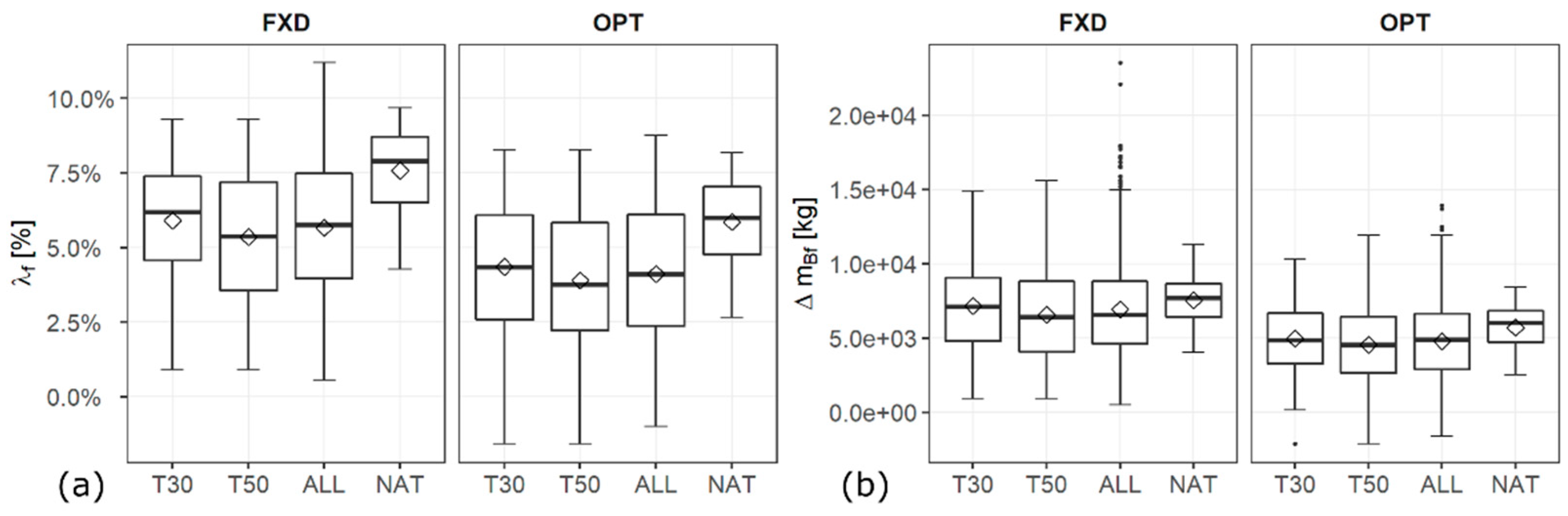
Figure 5 shows the relative (
) and absolute (
) formation efficiency metrics for the different studies and the different reference settings.
It can be observed, that if both, altitude and speed of the reference mission are constrained to the specification of the formation (setting FXD) the relative benefits increase as the reference mission is using more fuel than in the optimal case (setting OPT). For the global studies we estimated a difference of the average relative fuel savings between the two options in the range of 1.45–1.55% and for the average absolute fuel savings in the range of 2000–2200 kg. For the regional study we estimated a difference of around 1.72% for the relative and 1835kg for the absolute fuel savings. As the FXD setting represents comparable conditions for reference and formation missions it is more suitable to disentangle the climate effects and is, therefore, selected for further investigation within this study. However, in a real-world formation scenario, the reference flight would presumably choose an optimal flight profile and thereby indirectly reduce the AWSE benefits of the formation.
3.3. Route Geometry and Benefit Analysis
Figure 6 shows the relative (
) and absolute (
) efficiency metrics, detours (
) and relative lengths of the beneficial segment (
) for leader (orange) and follower (green) and the FXD setting for both the ALL and the NAT study. It can be observed, that for the relative and absolute benefits the follower generally consumes less, the leader more fuel while participating in an AWSE formation. This can be explained by the fact that the additional fuel consumption resulting from the detours, both formation members need to take to join the formation, are only compensated for the follower. The total benefit of the formation (red) turns out to be positive. The average values for both studies are presented in
Table 2.
The ALL study, in comparison to the NAT study, shows a considerably wider distribution of the values due to a greater range of FRG variance, as the formations in the NAT study generally are more similar to each other. This can be seen in the statistical distribution of the FRG parameters (see
Figure 6) as well. The spread of the values of the ALL study is generally larger than the spread of the values for the NAT study. For example, the average detours are at about 2.5% for the follower and 3.6% for the leader for the ALL study whereas in the NAT study the detours in average stay at around 0.8% for the leader and 1.1% for the follower. Furthermore, the distribution of the relative length of the beneficial segment
in the ALL study shows a considerably wider spread compared to the NAT study. The average length of the beneficial segment ranges between 75–90%, depending on position in the formation and study, indicating that long haul flights provide larger beneficial segments. In all studies, the follower shows a slightly shorter beneficial segment compared to the leader. Further investigation is needed to clarify if this is an effect caused by the selection process of the formation candidates or resulting from a different effect.
Figure 5 shows, that for the different global studies similar distributions of the relative benefits are obtained with average values
between 5% and 6% (FXD setting) resulting in average absolute savings
of about 6500 kg to 7200 kg of fuel per formation. Among the evaluated global studies, the T30 study was identified to achieve the highest relative benefits for the flights under evaluation. This is presumably a result of the airport selection, as the selected airports are located mainly in Europe, North America, the Middle East and Asia. Airports located geographically close to each other generally foster formations that are more profitable, since the length of the beneficial segment is maximized and detours are minimized. The mean values and standard deviations for the efficiency metrics, detours and beneficial segment lengths for all studies are presented in
Table 2. Here the T30 study shows the lowest detours and the highest formation segment lengths compared to the other global studies as well as the smallest standard deviations for almost all parameters. The ALL study shows the highest deviations which can be assumed to be a result of the higher variability of the FRGs due to the global extent of the study. Further investigation is needed to clarify this assumption.
For the NAT study the benefits generally turn out to be larger than for the global studies (see
Figure 6 and
Table 2) and the spread and standard deviations of the values are considerably lower than the values for the global studies. Here, as for the T30 study, the selection of origin and destination airports leads to more profitable formations with considerably lower detours, even when taking wind effects into account.
3.4. Formation Ranking
In order to get an idea of the fuel saving potential of AWSE in this chapter the five formations yielding the highest relative and absolute fuel savings found in the ALL study are shortly presented in
Table 3. We describe a formation by a double origin destination pair (DODP) given by the two origin (O) and destination (D) airports of the formation members (IATA airport codes) using a nomenclature as “O
ld-D
ld/O
fw-D
fw”.
The formation identified in the ALL scenario with the highest relative benefit turned out to be RUN-CDG/MRU-CDG originating from La Réunion (RUN) and Mauritius (MRU) going to Paris Charles-de-Gaulle airport (CDG) as common destination. This formation was estimated to reach a relative benefit of more than 11%. These high values can be explained by a very long AWSE segment (about 93–94% of the total route) and very small detours (0.2–0.3%).
While looking at the absolute benefits, the ranking shows a slightly different order. The formation with the highest estimated absolute fuel savings was identified to be IAH-DOH/DFW-DOH originating in Houston (IAH) and Dallas (DFW) going to Doha (DOH), saving about 23,530 kg of fuel in total followed by the formation with changed aircraft positions DFW-DOH/IAH-DOH with 22,087kg of estimated fuel savings.
3.5. Geographic Formation Distribution
For all studies we assessed the geographic distribution of the formations using global formation inventories. The formation inventories are derived by summing up the number of formations passing through a specific grid cell.
Figure 7 shows the corresponding inventories for the different studies within this paper. Note, that approach and continuation segments are not represented in these inventories.
It can be observed that the amount of formations strongly increases in the global scenarios (
Figure 7a–c), when more flights from more airports are considered and more opportunities for formation flight occur. As the scenario size grows from T30 to T50 to ALL, more formations occur in Asia, the Middle East and to the southern hemisphere. In all three global scenarios, a high formation density on the North Atlantic is recognizable (A). Note, that in all scenarios we only considered formations among B777 aircraft. The global maps may change if we had accounted for additional aircraft types in our analysis. Yet, the results can give a first hint on the geographical distribution of formation opportunities. The results presented in this paper show that, even when the aircraft are constrained to a single type, the NAFC as one of the most frequented airspaces of the world holds a high potential for formation flight, legitimating a closer look on this area. Another area with high formation densities we identified between Europe and the Middle East (B). Here, the big hub airports channel many flights from Europe to Asia, generating opportunities for pairing u aircraft.
As the NAT study is not based on real flight plan data the formation inventory (
Figure 7d) shows a more compact distribution reflecting the adaptive formation routing due to the weather patterns under evaluation. As the European airports examined in the study are located rather close to each other the geographic variance of the wind optimal rendezvous points for all combinations (C) is smaller than for the separation points [
21,
22]. An area with high formation occurrence forming a kind of formation corridor can be identified, beginning at the Irish Sea (C) to the US state Maine.
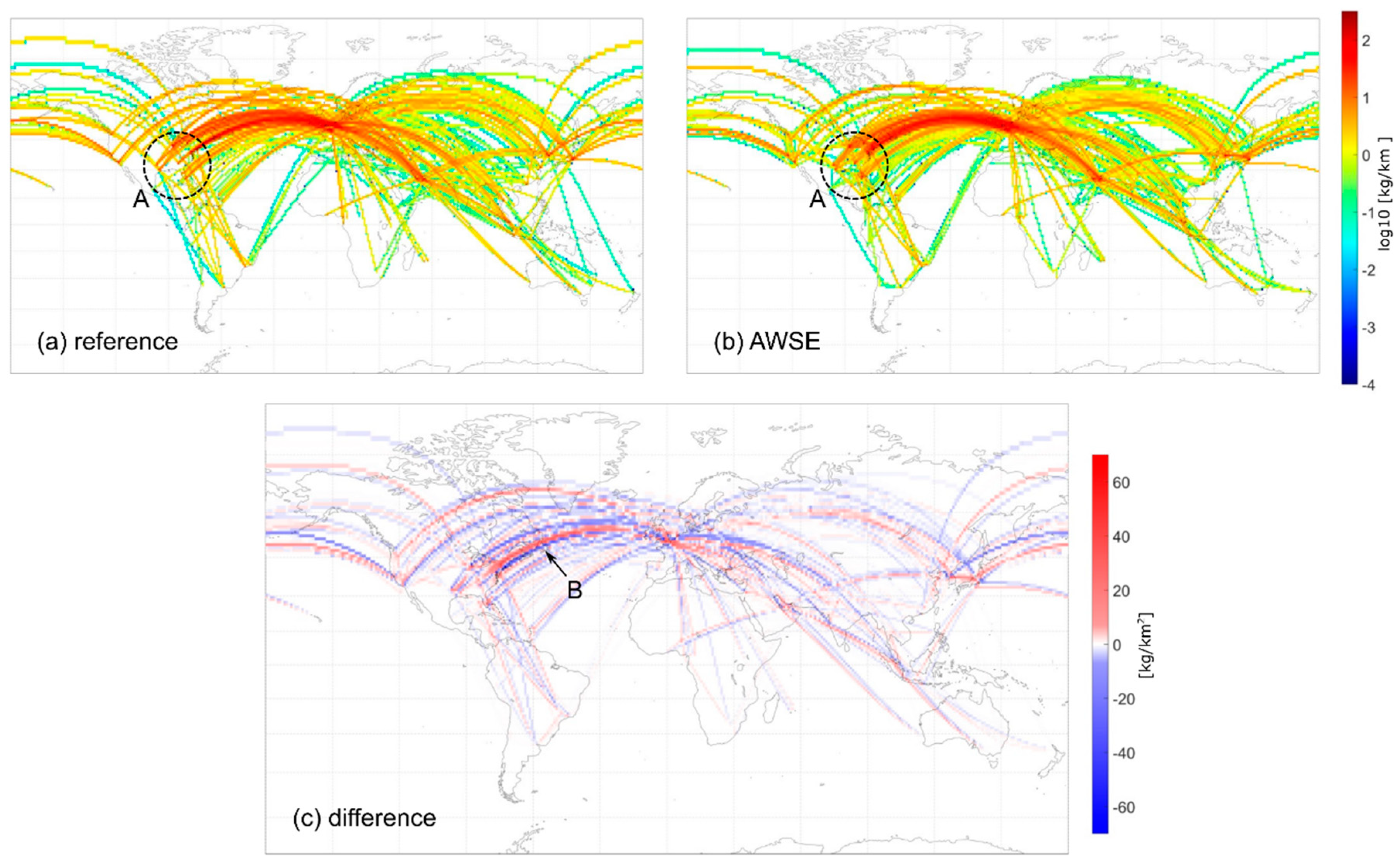
3.6. Emission Distribution
Figure 8 shows the inventories for the fuel consumption as a proxy for the emissions for the ALL study combined for leader and follower as well as for the reference and the AWSE scenario. For a better interpretability, a logarithmic scale is used. In the AWSE case (b), the flight tracks of both formation members are equal during the beneficial segment and only differ in the approach and continuation segments leading to a more condensed distribution of the fuel consumption compared to the reference scenario (a). Especially in North America, this merging of the fuel consumption in the AWSE scenario is clearly visible (A).
To further assess the difference between the AWSE and reference scenario,
Figure 8c shows an inventory of the differences in fuel consumption per grid cell using a linear scale. The shift of fuel consumption due to formation flight can clearly be identified in this figure with blue color indicating a decrease and red color indicating an increase accordingly. In the AWSE scenario both formation members may change their track in favor of the formation. The circumstance that both aircraft strive to minimize their detours and to maximize the benefits leads to the effect, that areas with decreasing and increasing emissions can be found to be situated close to each other. This effect is clearly visible, e.g., on the North Atlantic (B).
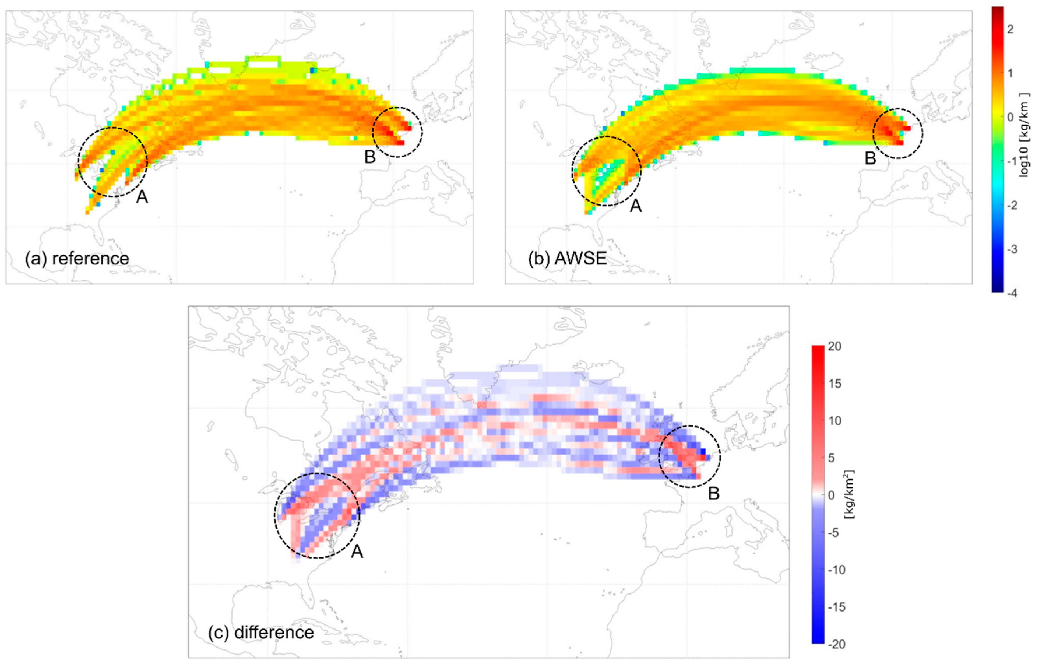
For the NAT study the corresponding fuel inventories are presented in
Figure 9. Analogous to
Figure 8, the locations of the fuel consumptions are merged together in the AWSE scenario compared to the reference scenario especially in the areas of approach and continuation of the formations (A, B). The overall geographic extend of the fuel consumption is slightly reduced as the routes are shifted in order to join the formations.
Figure 9c shows the inventory of the differences in fuel consumption for the NAT study using a linear scale. The above-mentioned effect of shifting the fuel consumption in favor of the formation routes can clearly be identified. Especially in the region of origin and destination airports, the approach and continuation segments of the formations drastically change the emission location (A, B).
3.7. Climate Impact
For the different studies and the FXD setting the resulting relative temperature responses
(see Equation (5)) in total are presented in
Figure 10a both for the leader, follower and the whole formation.
In all studies we found a positive effect of the AWSE scenario with respect to the reference scenario on the climate impact. In our analysis, the reduced contrail effect as well as the NOx effect is split evenly among the two formation partners. Hence, the leader also shows a reduced climate impact despite an increased fuel burn. The follower contributes even more to the effect as its fuel burn is additionally reduced by AWSE. The climate impact mitigation gains for the studies we performed averages out at about 22–24%. A more detailed analysis of the climate effects of formation flight is given by [
18], where implications for individual, direct, and indirect effects are presented.
Figure 10b shows the relative climate effect against the relative fuel saving benefits for the ALL and the NAT study. Here we identified a correlation for both studies, meaning that the more fuel is being saved (positive
) the more reduction of the climate effect is obtained (negative
). However, a strong variation of the values of
for the individual flights can be observed. This effect is presumably resulting from the geographic distribution of the formations and the variability of the underlying FRGs. In the NAT study this variation we found to be considerably lower than in the ALL study, as the routes are basically located in the same geographic region. However, the results imply that the construction of a surrogate model to assess the climate impact mitigation potential on the North Atlantic based on the FRG and the corresponding AWSE benefits might be feasible.
4. Discussion
The results show that formation flight and AWSE as a new operational procedure has a significant mitigation potential regarding the climate impact of aviation. Using current flight plans, we found that the fuel saving potential is already significant, even when limiting on a single aircraft type, as many opportunities for formation flight using AWSE for fuel saving were identified analyzing the data. Especially the region of the North Atlantic we found to hold a high potential for conducting AWSE as many opportunities for joining aircraft together can be expected while due to the close vicinity of the origin and destination airports detours can be minimized and AWSE duration maximized. However, it needs to be noted, that the overall climate mitigation potential of the new procedure we identified within our studies, needs to be interpreted in relation to all flights within the time period of evaluation.
The studies we conducted show in addition, that the climate impact mitigation potential of formation flight using AWSE can be expected to be even higher than the effects caused by the reduced fuel consumption of the follower aircraft alone. For a global scenario, we estimated the average climate impact reduction to be in the range of 22–24% while the fuel savings average out at about 5–6% for equivalent altitude and speed settings in the reference missions. This finding can be attributed to effects caused by overlying the two contrails of both formation members, as a notable shift of the geographic location of the emissions occurs from the single flights towards the joint formation routes. This implies that formation flight even without AWSE already might be reasonable from a climate impact mitigation perspective.
Furthermore, we found, that the correlation of the relative change in climate response and the fuel saving benefits especially on the North Atlantic region might allow for the creation of surrogate models predicting the fuel climate mitigation potential of a formation based on a set of simple parameters. However, further investigation is needed to confirm this assumption.
Another aspect that has to be mentioned is the fact, that due to the detours that both formation members need to take, the cash operating cost (COC) savings can be expected to be lower than the fuel savings alone. It will be interesting in future works to select formation candidates by COC or even direct operating costs (DOC) instead of fuel savings alone as it can be expected that this will result in different formation flight plans and hence lead to different emission scenarios.
As the studies we conducted were limited to a single aircraft type, future work will also include the simulation and analysis of larger scenarios, giving a more complete picture of the climate mitigation potential of formation flight and AWSE to substantiate the findings presented in this work while at the same time expanding our understanding of the relation between climate effects and scenario parameters.
Author Contributions
Conceptualization, T.M.; data curation: T.M., M.S., C.Z., and K.D., methodology, T.M., F.L., M.S., K.D., S.U., V.G. (Volker Grewe), S.M., C.Z., and H.Y.; writing—original draft preparation, T.M.; writing—review and editing, T.M., F.L., M.S., S.U., V.G. (Volker Grewe), and K.D.; visualization, T.M. and F.L.; project administration, V.G. (Volker Gollnick); funding acquisition, T.M., F.L., V.G. (Volker Gollnick), V.G. (Volker Grewe), and E.S. All authors have read and agreed to the published version of the manuscript.
Funding
This research was funded by the German Ministry of Economic Affairs and Energy (BMWi) under the National Aeronautical Research Programme (LuFo) V-2 under the grant agreement no. 20E1508A.
Institutional Review Board Statement
Not applicable.
Informed Consent Statement
Not applicable.
Data Availability Statement
Not applicable.
Conflicts of Interest
The authors declare no conflict of interest. The funders had no role in the design of the study; in the collection, analyses, or interpretation of data; in the writing of the manuscript, or in the decision to publish the result.
Abbreviations
The following abbreviations are used in the manuscript:
| AMS | Amsterdam Airport Schiphol, Netherlands |
| ATL | Hartsfield–Jackson Atlanta International Airport, USA |
| ATR | average temperature response |
| AVL | Athena Vortex Lattice |
| AWSE | aircraft wake-surfing for efficiency |
| BADA | Base of Aircraft Data |
| BDD | base drag database |
| CDG | Charles de Gaulle Airport, Paris, France |
| COC | cash operating cost |
| DOC | direct operating cost |
| DFW | Dallas Fort Worth International Airport, USA |
| DODP | double origin-destination pair |
| DOH | Hamad International Airport, Doha, Katar |
| DRD | drag reduction database |
| ECMWF | European Centre for Medium-Range Weather Forecasts |
| EFF | extended formation flight |
| FCA | formation cruise altitude |
| FCM | formation cruise Mach number |
| FRG | formation route geometry |
| IAH | George Bush Intercontinental Airport, Houston, USA |
| JFK | John F. Kennedy International Airport, New York, USA |
| LHR | Heathrow Airport, London, England |
| LHS | Latin Hypercube Sampling |
| LRC | long-range cruise speed |
| LTO | landing and take-off cycle |
| MRU | Sir Seewoosagur Ramgoolam International Airport, Mauritius |
| NAFC | North Atlantic flight corridor |
| NAT | North Atlantic |
| ORD | Chicago O’Hare International Airport, USA |
| RUN | Roland Garros Airport, La Réunion, France |
| SEP | separation end point |
| RSP | rendezvous start point |
| TCM | Trajectory Calculation Module |
| TOC | top of climb |
| TOD | top of descent |
References
- Wieselsberger, C. Beitrag zur Erklärung des Winkelfluges einiger Zugvögel. Z. Flugtech. Mot. 1914, 15, 225–229. [Google Scholar]
- Lissaman, P.B.S.; Shollenberger, C.A. Formation Flight of Birds. Science 1970, 168, 1003–1005. [Google Scholar] [CrossRef] [PubMed]
- Koloschin, A.; Fezans, N. Flight Physics of Fuel-Saving Formation Flight. In Proceedings of the AIAA Scitech 2020 Forum, Orlando, FL, USA, 6–10 January 2020. [Google Scholar]
- Erbschloe, D.; Carter, D.L.; Dale, G.A.; Doll, C.; Niestroy, M.A.; Marks, T. Operationalizing Flight Formations for Aerodynamic Benefits. In Proceedings of the AIAA Scitech 2020 Forum, Orlando, FL, USA, 6–10 January 2020. [Google Scholar]
- Beukenberg, M.; Hummel, D. Aerodynamics, Performance and Control of Airplanes in Formation Flight. In Proceedings of the 17st Congress of the International Council of the Aeronautical Sciences, Stockholm, Sweden, 9–14 September 1990; pp. 1777–1794. [Google Scholar]
- Vachon, M.J.; Ray, R.; Walsh, K.; Ennix, K. F/A-18 Aircraft Performance Benefits Measured During the Autonomous Formation Flight Project. In Proceedings of the AIAA Atmospheric Flight Mechanics Conference and Exhibit, Monterey, CA, USA, 5–8 August 2002. [Google Scholar]
- Pahle, J.; Berger, D.; Venti, M.; Faber, J.; Duggan, C.; Cardinal, K. A Preliminary Flight Investigation of Formation Flight for Drag Reduction on the C-17 Aircraft. In Proceedings of the Atmospheric Flight Mechanics Conference, Portland, OR, USA, 8–11 August 2011. [Google Scholar]
- Brown, N.; Hanson, C. Wake-Surfing: Automated Cooperative Trajectories; NASA Armstrong Flight Research Center: Edwards, CA, USA, 2017. [Google Scholar]
- Ribichini, G.; Frazzoli, E. Efficient coordination of multiple-aircraft systems. In Proceedings of the 42nd IEEE International Conference on Decision and Control (IEEE Cat. No.03CH37475), Maui, HI, USA, 9–12 December 2003; Volume 1, pp. 1035–1040. [Google Scholar]
- Rao, V.; Kabamba, P. Time-optimal graph traversal for two agents: When is formation travel beneficial? In Proceedings of the 2003 American Control Conference, Denver, CO, USA, 4–6 June 2003; Volume 4, pp. 3254–3259. [Google Scholar]
- Kent, T.; Richards, A. A Geometric Approach to Optimal Routing for Commercial Formation Flight. In Proceedings of the AIAA Guidance, Navigation, and Control Conference, Minneapolis, MN, USA, 13–16 August 2012. [Google Scholar]
- Hange, C. Evaluation of Formation Flight as a Fuel Reduction Strategy Given Real World Flight Dispatching Constraints. In Proceedings of the 2013 Aviation Technology, Integration, and Operations Conference, Los Angeles, CA, USA, 12–14 August 2013. [Google Scholar]
- Xue, M.; Hornby, G. An Analysis of the Potential Savings from Using Formation Flight in the NAS. In Proceedings of the AIAA Guidance, Navigation, and Control Conference, Minneapolis, MN, USA, 13–16 August 2012. [Google Scholar]
- Visser, H.G.; Santos, B.F.; Verhagen, C.M.A. A Decentralized Approach to Formation Flight Routing. In Proceedings of the ATRS World Conference, Rhodes, Greece, 23–26 June 2016. [Google Scholar]
- Boling, B.; Liu, Y.; Stumpf, E. Understanding Fleet Impacts of Formation Flight. In Proceedings of the 5th CEAS Air & Space Conference, Delft, The Netherlands, 7–11 September 2015. [Google Scholar]
- Flanzer, T.C.; Bieniawski, S.R.; Brown, J.A. Advances in Cooperative Trajectories for Commercial Applications. In Proceedings of the AIAA Scitech 2020 Forum, Orlando, FL, USA, 6–10 January 2020. [Google Scholar]
- Swaid, M.; Marks, T.; Lührs, B.; Gollnick, V. Quantification of Formation Flight Benefits under Consideration of Uncertainties on Fuel Planning. In Proceedings of the 31st Congress of the International Council of the Aeronautical Sciences, Belo Horizonte, Brazil, 9–14 September 2018. [Google Scholar]
- Dahlmann, K.; Matthes, S.; Yamashita, H.; Unterstrasser, S.; Grewe, V.; Marks, T. Assessing the Climate Impact of Formation Flights. Aerospace 2020, 7, 172. [Google Scholar] [CrossRef]
- Unterstrasser, S.; Stephan, A. Far field wake vortex evolution of two aircraft formation flight and implications on young contrails. Aeronaut. J. 2020, 124, 667–702. [Google Scholar] [CrossRef] [Green Version]
- Grewe, V.; Stenke, A. AirClim: An efficient tool for climate evaluation of aircraft technology. Atmos. Chem. Phys. Discuss. 2008, 8, 4621–4639. [Google Scholar] [CrossRef] [Green Version]
- Marks, T.; Swaid, M.; Lührs, B.; Gollnick, V. Identification of optimal rendezvous and separation areas for formation flight under consideration of wind. In Proceedings of the 31st Congress of the International Council of the Aeronautical Sciences, Belo Horizonte, Brasil, 9–14 September 2018. [Google Scholar]
- Marks, T.; Swaid, M. Optimal Timing and Arrangement for Two-Aircraft Formations on North Atlantic under Consideration of Wind. In Proceedings of the AIAA Scitech 2020 Forum, Orlando, FL, USA, 6–10 January 2020. [Google Scholar]
- Drews, K.; Marks, T.; Konieczny, G.; Linke, F.; Gollnick, V. Identification and Modeling of Civil Formation Flight Routes Based on Global Flight Schedule Data. In Proceedings of the 66. Deutscher Luft- und Raumfahrtkongress (DLRK), Munich, Germany, 5–7 September 2017. [Google Scholar]
- Marks, T. Modellansätze zur Bewertung von Formationsflügen im Lufttransportsystem. Ph.D. Thesis, Hamburg Technical University, Hamburg, Germany, 2019. [Google Scholar]
- Linke, F. Trajectory Calculation Module (TCM)—Tool Description and Validation; Internal Report; German Aerospace Center: Hamburg, Germany, 2014. [Google Scholar]
- Lührs, B.; Linke, F.; Gollnick, V. Erweiterung eines Trajektorienrechners zur Nutzung meteorologischer Daten für die Optimierung von Flugzeugtrajektorien. In Proceedings of the 63. Deutscher Luft- und Raumfahrtkongress (DLRK), Augsburg, Germany, 16–18 September 2014. [Google Scholar]
- Zumegen, C.; Stumpf, E. Flight behaviour of long-haul commercial aircraft in formation flight. In Proceedings of the Air Transport Research Society, ATRS World Conference, Amsterdam, The Netherlands, 2–5 July 2019. [Google Scholar]
- Marks, T.; Zumegen, C.; Gollnick, V.; Stumpf, E. Assessing formation flight benefits on trajectory level including turbulence and gust. In Proceedings of the Italian Association of Aeronautics and Astronautics XXV International Congress, Rome, Italy, 9–12 September 2019. [Google Scholar]
- Dubois, D.; Paynter, G.C. “Fuel Flow Method2” for Estimating Aircraft Emissions; SAE International: Warrendale, PA, USA, 2006. [Google Scholar]
- Dahlmann, K.; Grewe, V.; Frömming, C.; Burkhardt, U. Can we reliably assess climate mitigation options for air traffic scenarios despite large uncertainties in atmospheric processes? Transp. Res. Part D Transp. Environ. 2016, 46, 40–55. [Google Scholar] [CrossRef] [Green Version]
- Unterstrasser, S. The Contrail Mitigation Potential of Aircraft Formation Flight Derived from High-Resolution Simulations. Aerospace 2020, 7, 170. [Google Scholar] [CrossRef]
- Irvine, E.; Hoskins, B.J.; Shine, K.P.; Lunnon, R.W.; Froemming, C. Characterizing North Atlantic weather patterns for climate-optimal aircraft routing. Meteorol. Appl. 2012, 20, 80–93. [Google Scholar] [CrossRef] [Green Version]
Figure 1.
Migratory birds flying in a typical V-shaped formation (photography by Tobias Marks).
Figure 1.
Migratory birds flying in a typical V-shaped formation (photography by Tobias Marks).
Figure 2.
Basic principle of a two-aircraft formation performing AWSE as assumed within this work.
Figure 2.
Basic principle of a two-aircraft formation performing AWSE as assumed within this work.
Figure 3.
General approach as followed in this paper. The two study branches are merged together for the detailed recalculation and the climate assessment of the identified formations.
Figure 3.
General approach as followed in this paper. The two study branches are merged together for the detailed recalculation and the climate assessment of the identified formations.
Figure 4.
General construction of formation route geometry (FRG) with approach and continuation segments (black), reference tracks (gray) and beneficial segment (blue); RSP adaption due to timing constraints (orange) and qualitative representation of a rendezvous line (green).
Figure 4.
General construction of formation route geometry (FRG) with approach and continuation segments (black), reference tracks (gray) and beneficial segment (blue); RSP adaption due to timing constraints (orange) and qualitative representation of a rendezvous line (green).
Figure 5.
Comparison of the benefits for the different settings and studies. Relative efficiency metric (a), absolute efficiency metric (b); mean values (diamond).
Figure 5.
Comparison of the benefits for the different settings and studies. Relative efficiency metric (a), absolute efficiency metric (b); mean values (diamond).
Figure 6.
Histograms and mean values of the relative () and absolute () formation efficiency metrics, detours (), relative lengths of the beneficial segment () for the FXD setting; leader (orange), follower (green), combined (red); note: occurrence is shown on y-axis.
Figure 6.
Histograms and mean values of the relative () and absolute () formation efficiency metrics, detours (), relative lengths of the beneficial segment () for the FXD setting; leader (orange), follower (green), combined (red); note: occurrence is shown on y-axis.
Figure 7.
Formation inventories for all studies: T30 (a), T50 (b), ALL (c) and NAT (d). Note: scale of NAT study differing from others. Note: the rasterization effect is due to the cell size of the inventories.
Figure 7.
Formation inventories for all studies: T30 (a), T50 (b), ALL (c) and NAT (d). Note: scale of NAT study differing from others. Note: the rasterization effect is due to the cell size of the inventories.
Figure 8.
Inventories for fuel consumption for the ALL study and the FXD setting combined for leader and follower. Reference scenario (a), AWSE scenario (b); Inventory for difference in fuel consumption for the ALL study and the FXD setting, combined for leader and follower (c). Note: the rasterization effect is due to the cell size of the inventories.
Figure 9.
Inventories for fuel consumption for the NAT study and the FXD setting combined for leader and follower. Reference scenario (a), AWSE scenario (b); Inventory for difference in fuel consumption for the NAT study and the FXD setting (c). Note: the rasterization effect is due to the cell size of the inventories.
Figure 10.
Relative temperature responses for the FXD setting separated by leader, follower and formation for the studies performed within this work (a); against for the ALL and NAT scenarios with regression lines (b).
Figure 10.
Relative temperature responses for the FXD setting separated by leader, follower and formation for the studies performed within this work (a); against for the ALL and NAT scenarios with regression lines (b).
Table 1.
General statistics for the different scenarios assessed in this study.
Table 1.
General statistics for the different scenarios assessed in this study.
| | T30 | T50 | ALL | NAT |
|---|
| single flights after filtering | 10,457 | 16,503 | 32,939 | n/a |
| beneficial formations | 2701 | 5599 | 16,046 | n/a |
| selected formations | 1122 | 1878 | 4569 | n/a |
| unique formations | 155 | 292 | 795 | 648 |
| feasible/selected formations | 100 | 203 | 555 | 334 |
| single flights | 1434 | 2558 | 6564 | 668 |
| percentage | 13.7 | 15.5 | 19.9 | n/a |
Table 2.
Average statistics for the different scenarios assessed in this study and the FXD setting.
Table 2.
Average statistics for the different scenarios assessed in this study and the FXD setting.
| | | T30 | T50 | ALL | NAT |
|---|
| | | Mean | sd | Mean | sd | Mean | sd | Mean | sd |
|---|
| [%] | 5.9 | 1.96 | 5.35 | 2.22 | 5.66 | 2.28 | 7.57 | 1.34 |
| [kg] | 7162 | 3066 | 6555 | 3137 | 6923 | 3401 | 7536 | 1494 |
| [%] | 3.25 | 3.25 | 3.75 | 3.66 | 3.57 | 3.66 | 0.81 | 1.48 |
| [%] | 2.30 | 2.52 | 2.93 | 2.66 | 2.52 | 2.62 | 1.1 | 2.13 |
| [%] | 88.50 | 3.77 | 88.09 | 3.58 | 88.27 | 3.83 | 81.54 | 7.51 |
| [%] | 79.13 | 11.59 | 78.41 | 11.81 | 77.29 | 12.71 | 78.08 | 8.02 |
Table 3.
Ranking of DODPs by and for the ALL study and the FXD setting.
Table 3.
Ranking of DODPs by and for the ALL study and the FXD setting.
| DODP | Rank by | [%]
| Rank by | [kg]
| [%]
| [%]
| [%]
| [%]
|
|---|
| RUN-CDG/MRU-CDG | 1 | 11.184 | 3 | 17,954 | 0.323 | 0.213 | 94.22 | 93.55 |
| IAH-DOH/DFW-DOH | 2 | 10.964 | 1 | 23,530 | 0.279 | 0.585 | 94.80 | 95.91 |
| LHR-GRU/CDG-GRU | 3 | 10.500 | 6 | 17,254 | 0.986 | 0.155 | 92.49 | 93.81 |
| DFW-DOH/IAH-DOH | 4 | 10.292 | 2 | 22,088 | 2.183 | 0.009 | 95.28 | 95.94 |
| FRA-SGN/CDG-BKK | 5 | 9.961 | 9 | 16,605 | 0.816 | 0.106 | 86.76 | 89.32 |
| MRU-CDG/RUN-CDG | 6 | 9.882 | 5 | 17,725 | 0.243 | 0.274 | 93.65 | 94.39 |
| ATL-DXB/IAD-AUH | 13 | 9.327 | 4 | 17,846 | 0.055 | 2.573 | 90.87 | 95.04 |
| Publisher’s Note: MDPI stays neutral with regard to jurisdictional claims in published maps and institutional affiliations. |
© 2021 by the authors. Licensee MDPI, Basel, Switzerland. This article is an open access article distributed under the terms and conditions of the Creative Commons Attribution (CC BY) license (http://creativecommons.org/licenses/by/4.0/).

 ,
, 


