
Tuning of a Linear-Quadratic Stabilization System for an Anti-Aircraft Missile


Faculty of Mechatronics, Armament and Aerospace, Military University of Technology, Gen. S. Kaliskiego 2 Street, 00-908 Warsaw, Poland
Aerospace 2021, 8(2), 48; https://0-doi-org.brum.beds.ac.uk/10.3390/aerospace8020048
Submission received: 30 September 2020
/
Revised: 31 January 2021
/
Accepted: 9 February 2021
/
Published: 12 February 2021
Abstract
:A description is given of an application of a linear-quadratic regulator (LQR) for stabilizing the characteristics of an anti-aircraft missile, and an analytical method of selecting the weighting elements of the gain matrix in feedback loop is proposed. A novel method of LQR tuning via a single parameter was proposed and tested. The article supplements and develops the topics addressed in the author’s previous work. Its added value includes the observation that the solutions obtained are symmetric pairs, and that the tuning parameter proposed for the designed linear-quadratic regulator enables the selection of suitable parameters for the airframe stabilizing loop for the majority of the analytical solutions of the considered Riccati equation.
1. Introduction
In anti-aircraft missile homing systems equipped with both mechanically and electronically controlled seekers, one observes a phenomenon of the impact of the airframe oscillations on the operation of the tracking systems. Due to the imperfect disturbance rejection performance, missile motion may severely degrade the tracking accuracy [1,2,3,4,5]. This situation is particularly disadvantageous during the terminal guidance phase, as it requires a very rapid reaction on the part of the missile, involving significant rotations of its airframe. In extremely unfavorable tactical conditions—despite the use of an adequate seeker stabilization loop—the target tracking process may break. It therefore becomes necessary to identify solutions enabling stabilization of the operating conditions of the on-board seeker [6,7,8]. They are often designed using adaptive linear control, which has certain benefits.
Adaptive linear control is an important component of autonomous vehicle control systems, in which case linear approximations are useful for analysis and design [9]. Linear theory is successfully used for the analysis and synthesis of control systems even though most real systems are nonlinear. The field of linear systems has been declared many times to be exploited and obsolete from a research point of view, but interest has repeatedly been renewed due to new viewpoints and the introduction of new theories [9,10]. Recently, an interest in linear adaptive control in missile and space technology can be observed, where adaptive-tuned PID [11,12,13,14], FPID [11,15,16,17] and linear-quadratic regulator (LQR) [18,19,20,21,22,23,24,25] controllers are widely proposed.
Recent research has focused on satisfying performance and stability robustness requirements by designing missile autopilots using optimal control theory [18,23]. These requirements for current and future missiles are crucial because of the necessity to use multivariable digital flight control systems [26], which in turn are dictated by the conditions of the modern air battlefield. In this context, LQR state feedback designs are generally perceived as providing good performance characteristics and stability margins, with the availability of the states required for implementation [18,22]. Thus, in the literature, linear-quadratic regulators are proposed for both integrated missile guidance systems and the stabilization of their individual components. For example, in [19] the use of an LQR was considered wherein entries of the weighting matrix were chosen as an inverse function of the range-to-go, on the assumption that it is possible to construct a feedback linearized dynamic system from a simulation model of the missile at every value of the state automatically. In [20], a time-varying LQR design method was proposed to deal with the various disturbances in the hypersonic vehicle reentry profile, by calculating the weighting matrices constructed based on the Bryson principle using time-varying parameters. As opposed to classical approaches, the actual states of the flight system were employed to calculate the parameters in weighting matrices. The LQR method is also applied in [21] as a solution for the anti-tank missile guiding process and determines the commands controlling the fin deflections and the thrust vector via continuously calculating Jacobians. In turn, in [18], the LQR formulation is the same, but it was extended to describe the full-state feedback robust integral servo controller equations. The article [24] illustrates that in order to stabilize a highly unstable missile airframe and achieve the required performance, a hybrid of two control schemes may be used. In this case, a state feedback linear quadratic regulator was proposed to stabilize the plant and a forward path optimal controller was used to achieve the required performance and robustness. Several papers describe the use of an LQR as a part of the missile stabilization system; e.g., [25] discusses a cascaded LQR controller for effective roll stabilization of the missile autopilot in a realistic model; robust missile roll autopilot design with an LQR application for solving the flexible airframe dynamics is also discussed in [23]; and in [7] LQR was chosen as an equivalent part of the sliding mode control (SMC) airframe stabilization system. These selected examples show the multitude of possible LQR applications in aerospace and missile technology.
In the case of a linear time-invariant (LTI) system, the gain coefficients of a linear-quadratic controller used in a feedback loop can usually be determined without difficulty. The problem becomes more complicated when the system analyzed contains nonstationary and nonlinear features. This situation occurs, among others, when guiding the missile against an aerial target. The lack of stationarity of the airframe dynamics determines the properties of the whole guidance loop, and can lead to a loss of stability of the entire system. In the case under consideration, when solving the Riccati equation to find the gain coefficients for a missile autopilot feedback loop, numerical computation methods can be applied to a set of static values describing the state of the “frozen” system (i.e., at the moment—for a short finite-time horizon). The fundamental difficulty with this approach is the necessity for the computations to be carried out in real time [19,27]. There are also certain technical hitches related to the software implementation, e.g., the weak conditioning of the matrices [7,8]. It is therefore valuable to find an analytical solution of the controller, which ensures adaptability according to the state of the system.
In this paper, an adaptive linear-quadratic stabilization system is considered for which a novel method of tuning via a single tuning parameter was proposed and tested. Reducing the stabilization system settings to the case of a single parameter seems attractive from a practical point of view. The main effort is focused on analyzing obtained solutions in detail and describing a procedure for selecting appropriate values of the LQR tuning parameter for the proposed airframe stabilization system. In the author’s previous work, an initial concept of achieving an analytical solution of a time-varying linear-quadratic stabilization system was proposed and tested. A basic formula of feedback loop gain matrix equations (without a tuning parameter) was introduced and used as a part of the SMC stabilization system in [7].
It has been shown that the proposed solution provides a favorable effect on the operating conditions of the seeker and a reduction in energy losses resulting from oscillations of the airframe. In turn, [8] signaled the possibility of introducing a single tuning parameter and improving the performance of the designed airframe stabilization system. The main contributions of this paper include: (a) a comparative analysis of the analytical solutions of a time-varying linear-quadratic airframe stabilization system; (b) a procedure for selecting appropriate tuning parameter values; and (c) an observation that the solutions obtained are symmetric pairs, which on the one hand confirms the correctness of the calculations, and on the other introduces the possibility of narrowing the range of the sought settings of the LQR tuning parameter.
The paper is organized as follows. The problem is formulated in Section 2.1. The missile’s airframe dynamics model’s description is given in Section 2.2. The draft of the stabilization system design is discussed in Section 2.3. The tuning procedure is presented in Section 2.4. Issues related to numerical computation methods are described in Section 2.5. To show the features of the proposed solutions, numerical simulations were performed, and their results are given in Section 3. Finally, Section 4 offers some conclusions.
2. Methods
2.1. Problem Formulation
When guiding a missile towards an aerial target, it is requested that
namely, the angular rate of the airframe should be equal to the angular rate of the missile’s velocity vector, and not depend on the dynamics of the missile itself [6,7,8]. This requirement, impossible to fulfill in practice however, leads to the conclusion that the absolute rotation angle of the airframe should be approximately equal to the absolute rotation angle of the missile velocity vector; i.e.,
Obtaining equality given by Equation (2) depends on the system’s ability to reduce the effect of the components related to the dynamics of the missile airframe. The left side of the Equation (2) will be close to the right side when the transitional processes occurring during guidance are shorter and less oscillatory. Minimizing the value of the left side of Equation (2) is the task of the designed adaptive linear-quadratic stabilization system.
In the classical approach, the infinite horizon LQR settings are determined based on linear dynamic equations and a quadratic cost function in the form
where and are symmetric, positive (semi-positive) definite matrices of weighting parameters for the state vector and the control vector , respectively. In general, there are no unified methods of selecting the and entries; however, several approaches can be found in the literature [21,27,28,29,30,31,32,33,34,35,36], usually based on modified (e.g., time-varying) Bryson principle or “trial and error” methods. The main problem connecting all of these is the need to define the values of and to find the solution of the feedback gain matrix .
In this study, determining the entry values of matrix is not necessary. Instead, a novel method is proposed by introducing a single tuning parameter into equations describing the entries of gain matrix , allowing the change of LQR performance. A linear-quadratic controller is applied to a cruciform, canard-controlled, roll-stabilized missile, treated as a SIMO (single-input, multi-output) system, in which control command u is the input signal and the airframe angular rate and angle of attack are the output signals. The motion of such a missile can be separated into two perpendicular channels, and the problem can be treated as planar in each of these channels.
2.2. Missile Airframe Dynamics
As mentioned above, the study relates to a cruciform, canard-controlled, roll-stabilized missile. The stabilization loop in the roll control plane is assumed to be ideal. Using this assumption, its motion can be separated into two perpendicular channels and analyzed independently. The equation of motion relative to an axis normal to the velocity vector is obtained by projecting the forces acting on the missile onto that axis. The equation of rotational motion is obtained by balancing the moments of forces acting on the missile. This is a typical approach to missile dynamics model determination and it can be found in the form presented or a similar form in a number of research papers [6,37,38,39,40,41,42,43,44,45,46]. Neglecting the gravitational force, for the after-burning phase of flight, the dynamics of the missile in the control plane are described by the equations:
The symbols in Equations (4)–(7) have the following meanings: m is the missile mass (kg); I is the missile moment of inertia (kg·m); V is the module missile velocity vector (m/s); is the airframe angular rate (rad/s); is the angle of attack (rad); is the angle of the missile velocity vector in control plane (rad); S is the reference area (m); l is the reference length (m); is the air density (kg/m); is the canard servo time constant (s); and are actual and commanded canard deflections (rad), respectively; is induced drag coefficient (–); and is the zero-lift drag coefficient (–). The variables described by the common symbol represent derivatives of the missile nonlinear aerodynamic coefficients, where subscript M describes moment related components and subscript L is the lift force related component, as follows:
The force and moment coefficients describing the airframe aerodynamics have complex forms, whose derivations lie outside the scope of this work and will not be considered here. Polynomial approximations are taken for Mach’s number , and the following are assumed to hold
Noting that
where is the airframe rotation angle in the control plane (rad), the following equivalent for Equations (4) and (5) can be obtained:
For controller design purposes, and for reasons of simplicity, it is assumed that ; i.e., the inertia of the canards is ignored. Taking this into account, approximate dynamics, which will be used for the design of the linear-quadratic stabilization system, can be described by linearized vector-matrix equations as
where
The entries of matrices and are assumed to have the following forms:
2.3. Stabilization System Design
Using Equation (3), by the variation method of the optimal control theory, the feedback gain matrix can be obtained as follows:
where is the stabilizing solution of the Riccati equation
Let us take the matrices and to be
Scaling for single-input systems results only in the same amount of scaling on . In the case under consideration, was therefore chosen. Assuming that
the expanded form of the Equation (17) can be obtained as
In previous work [7,8], a complete solution was given for the controller in question. Here, a draft is presented for the sake of brevity. By summation of the matrices in Equation (20), rearrangement and while noting that , the system of equations takes the form:
By multiplying both sides of the second line in Equation (21) by 2 and summing, we have
The values of and are positive-defined and can be freely chosen by the designer. Let us assume that
There are two possible solutions of Equation (23)
By using Equation (24) to solve the system in Equation (21), with Equation (16), after some transformations, eight pairs of entries for the matrix can be found as follows:
where is treated as a tuning parameter of the proposed controller, and and are functions given as
Based on Equation (16) and Equations (25)–(30), the control law can be defined as
where is one of the feedback gain matrices given by Equations (25)–(28). The following expressions are used as the feed-forwarding scaling factors of the input signal (cf. Appendix A):
with . Due to the application specifics, the condition is always met.
2.4. LQR Tuning Procedure
The choice of the tuning parameter value for the particular feedback loop gain matrix is determined on the basis of Equation (2) and three additional quantity indices, defined as
in which A, and X are given as
where a is the normal acceleration of the airframe (m/s), is the angle of attack (rad) and is the number of signal samples considered.
The quantity index enables the detection of oscillations of the airframe in response to a step canard-fin deflection: in the case where the instantaneous value of the normal acceleration of the airframe is smaller than the value of that acceleration at the previous instant, the value of is increased by 1.
The index is used to detect over-regulation in the stabilization system. Over-regulation is examined based on the angle of attack (in view of the dynamic properties of the system, it is inappropriate to detect over-regulation using the airframe’s angular rate ). The reference value is taken to be the angle of attack at instant N, for which it is known a priori that the steady state of the system was achieved.
The index , in turn, is useful in determining the speed of the airframe’s response to a step canard-fin deflection. The value of the index is increased by 1 for every instant n greater than for which the airframe’s angle of attack does not attain 95% of the value of the angle of attack in the steady state . In the numerical simulations, was set equal to 1500, which corresponds to a time of 0.15 s for a sampling frequency of = 10 kHz.
The tuning parameter waa s selected according to the following rules. For chosen value of : (a) the absolute airframe rotation angle given by Equation (2) takes the minimum value; (b) the quality indices and take the minimum values in the considered range. The quality index plays an auxiliary role and establishes that the response of the airframe in the considered case may be slower than the required one. In the case of missiles number 6 and number 7, the values of were chosen arbitrarily, because the obtained values of the quality indices did not make it possible to clearly indicate the solutions, and the responses of the tested airframes were mostly unstable. To make a decision in this case, the values of the absolute rotation angle obtained for the individual values of the tuning parameter were used.
With respect to the tuning procedure, an iterative method was investigated for the response of the missile airframe to stepped canard-fin deflections. Calculations were performed for a set of coefficients defined in Equation (15) with constant values, describing the system state in a short-time horizon, for the instant of commencement of the terminal phase of missile guidance to an aerial target.
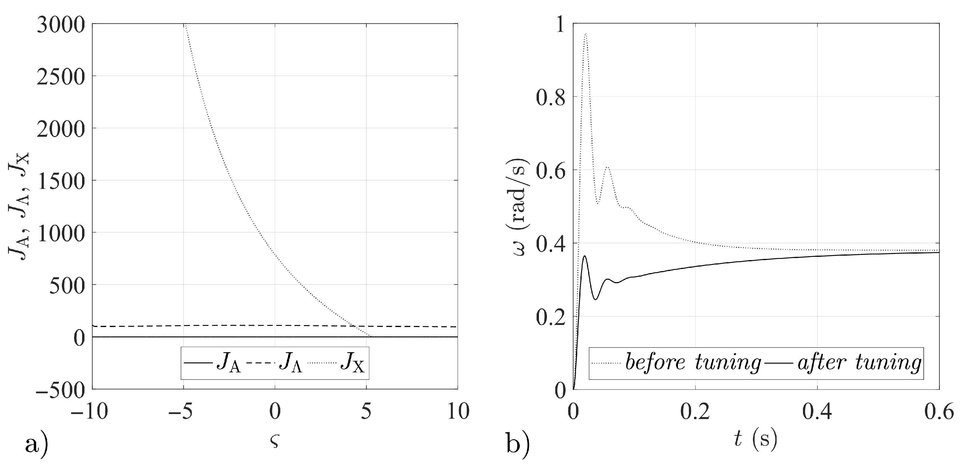
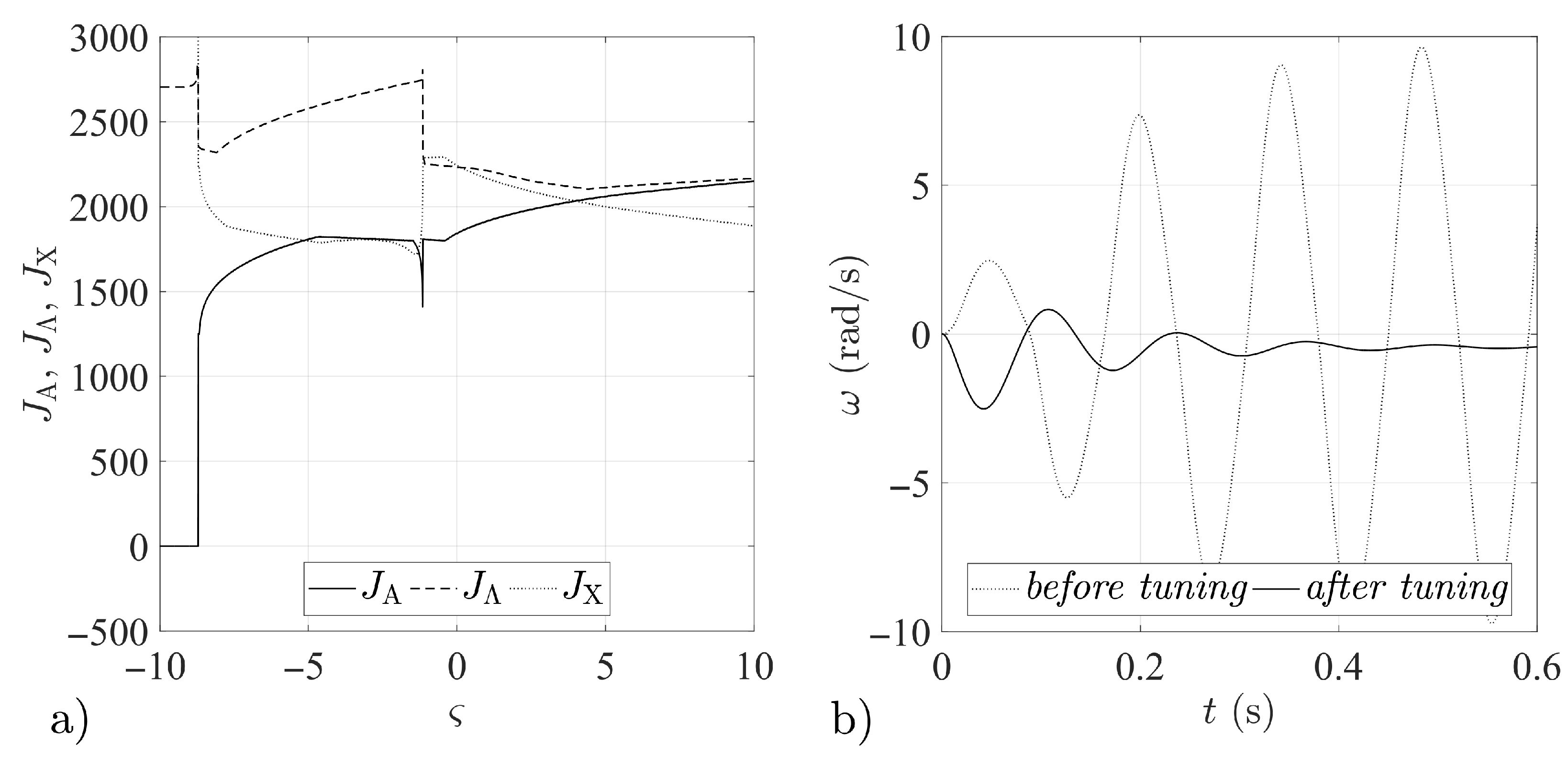
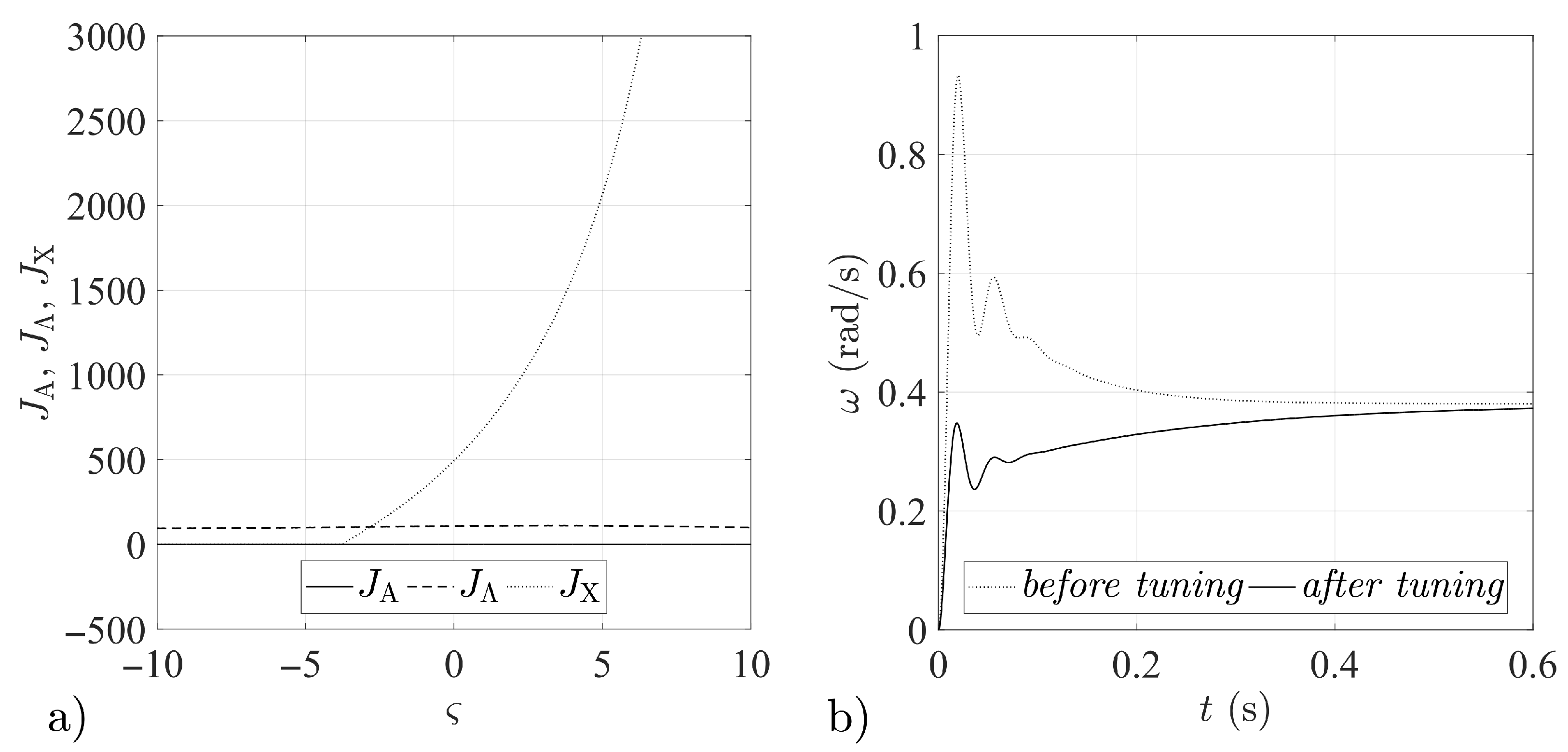
As it can be deduced from [7], setting an initial value of = 1 gives a good start point for the beginning of the LQR tuning procedure. Figure 1, Figure 2, Figure 3, Figure 4, Figure 5, Figure 6, Figure 7 and Figure 8 show the results of numerical computations for the different forms of the gain matrix implemented in the stabilizing loop, and the values taken for the airframe coefficients: s, s, s, s.
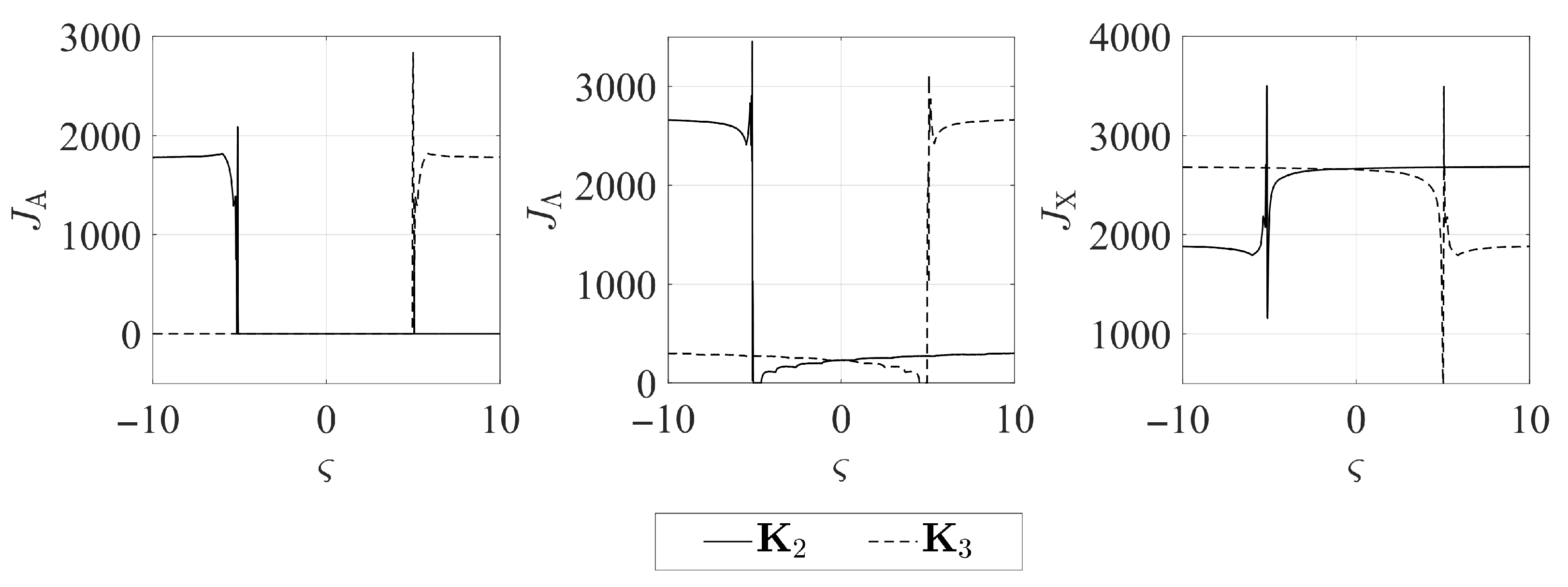
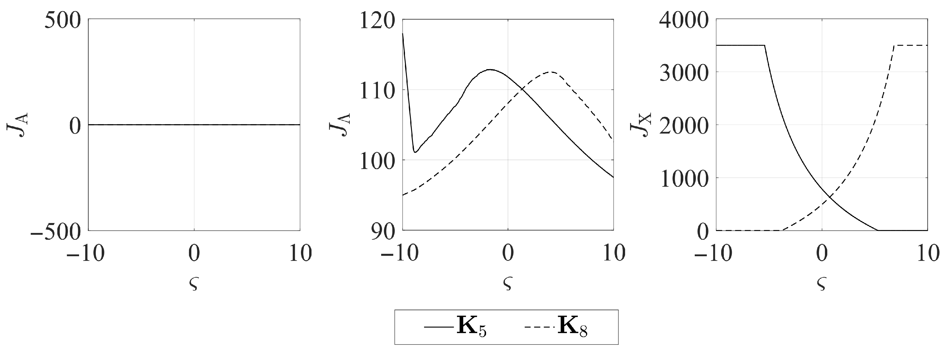
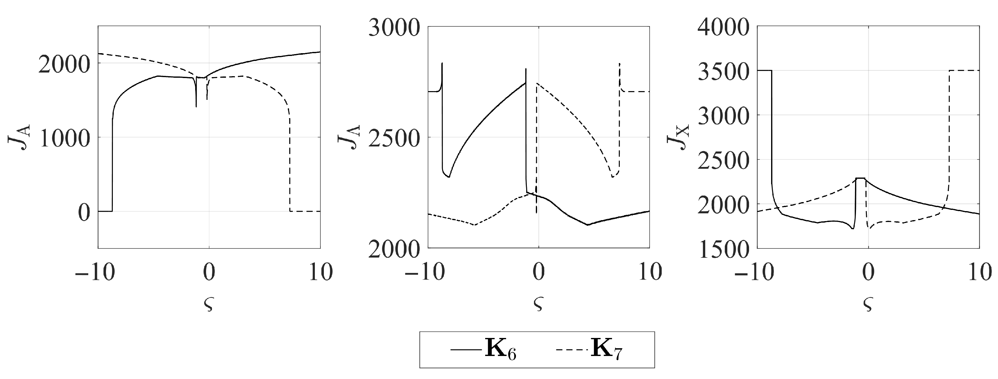
In Figure 1, Figure 2, Figure 3, Figure 4, Figure 5, Figure 6, Figure 7 and Figure 8, the results obtained for the quantity indices defined by Equation (33) are shown only in the range , due to the fact that the numerical analysis did not reveal any significant changes in the functioning of the analyzed stabilization systems outside that range (relative to the results attained for the boundary values of the assumed range of variation of the parameter ).
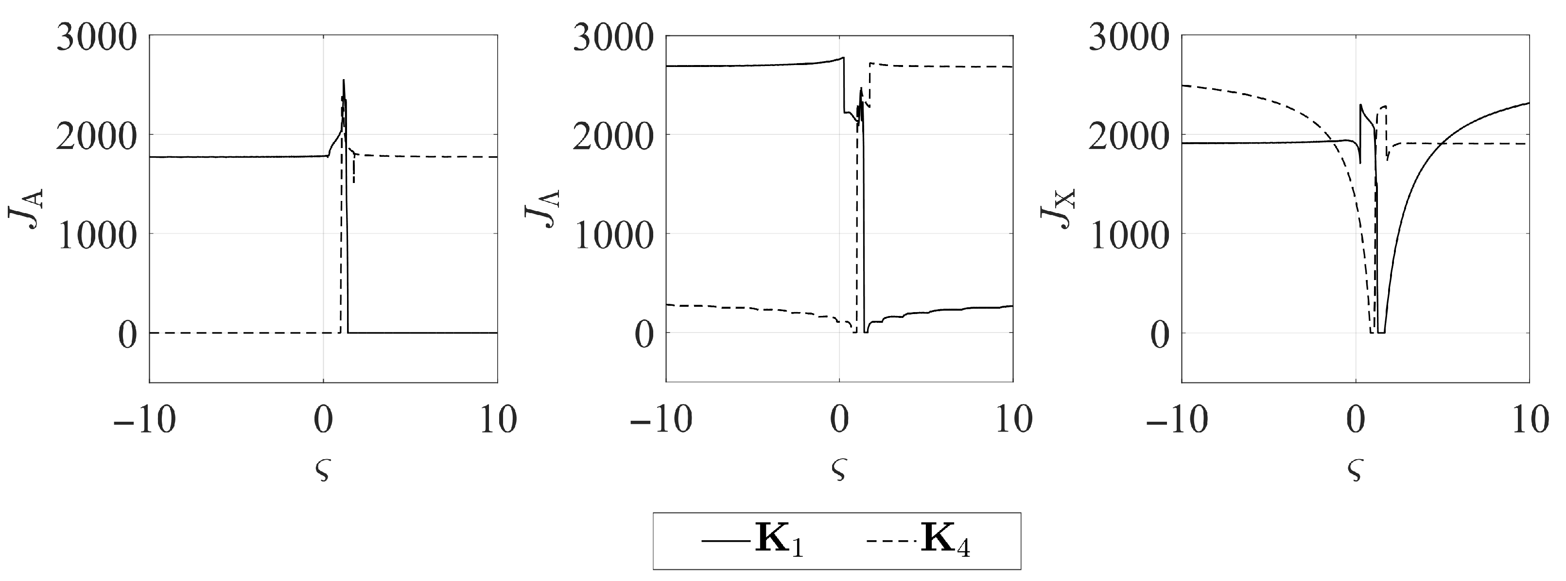
The numerical simulations revealed symmetries between the forms of the quantity indices determined for particular gain matrices (compare Figure 1a and Figure 4a, Figure 2a and Figure 3a, Figure 5a and Figure 8a, Figure 6a and Figure 7a). It may thus be assumed that the matrices given by Equations (25)–(28) form symmetric pairs of solutions, namely: – (with the axis of symmetry passing through the point = 1.25), – (with axis of symmetry = −0.045), – (with axis of symmetry = 0.79) and – (with axis of symmetry = −0.73). This is illustrated in detail in Figure 9, Figure 10, Figure 11 and Figure 12.
This fact suggests that the sought values of the tuning parameter should be distributed symmetrically with respect to those axes, i.e., . Indeed, the tuning values determined numerically based on the indices (33) for particular forms of the matrices given by Equations (25)–(28) satisfy that relationship (cf. Table 1).
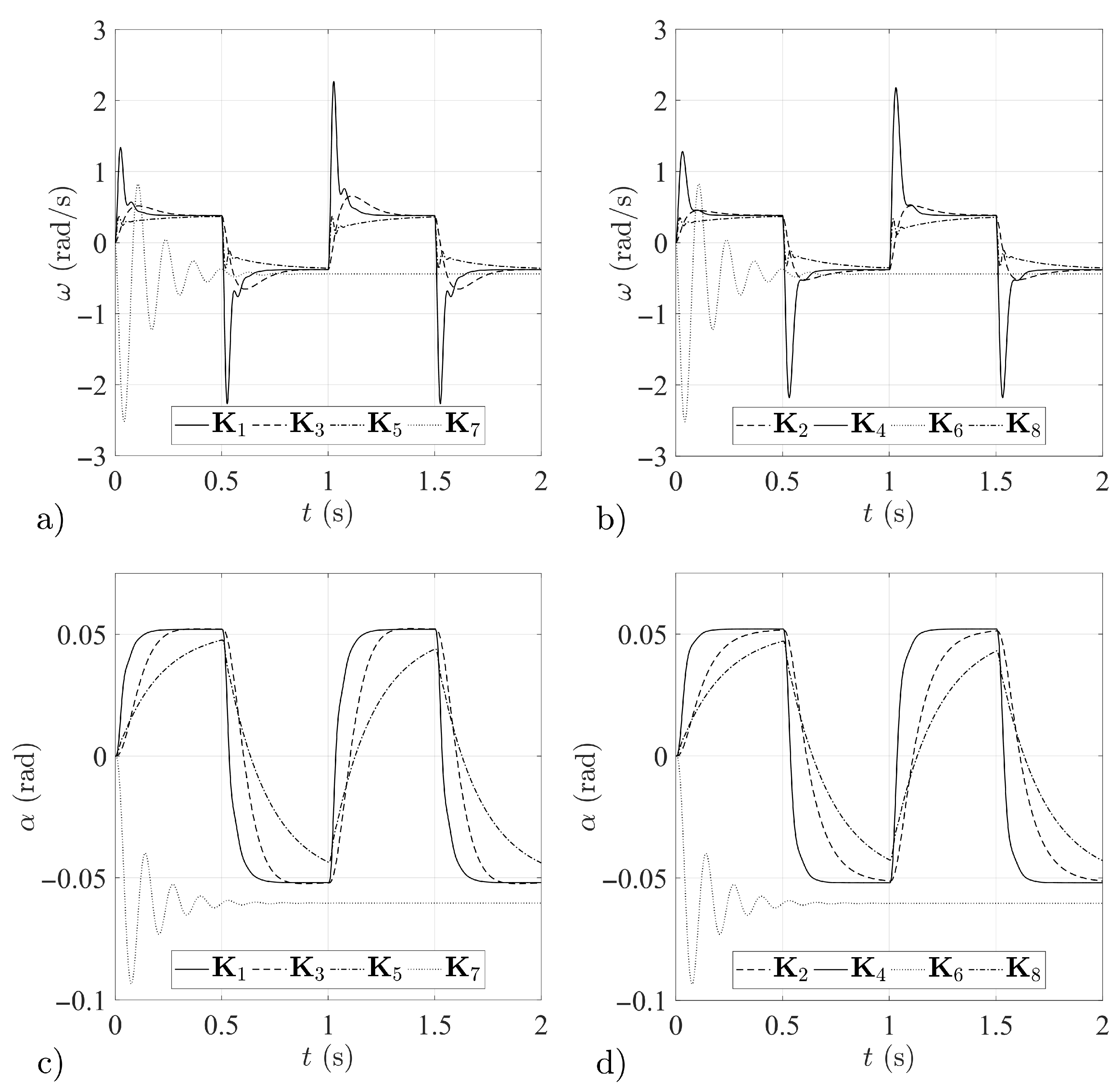
Figure 13 shows the graphs of angular rates and angles of attack obtained as a result of the response of missile airframes with stabilization systems using the matrices – to an applied test signal. A symmetric rectangular signal with values ±0.3 rad and a 50% duty cycle was input to the system, simulating stepped, alternating canard-fin deflections.
The following conclusions can be drawn from the results obtained.
Stabilization system solutions using the gain matrices – ensure a correct reaction to the applied input signal. In the case of stabilization systems configured based on the matrices and , smooth graphs are obtained with the required response dynamics, although it should be noted that the system with the matrix exhibits slightly higher inertia, which may lead to poorer results for missile guidance to an aerial target of high maneuverability. The graphs of airframe angular rates in the case of stabilization systems with the matrices and suggest that missiles with these systems will respond very rapidly to all changes in the input signal, but this may lead to oscillations if changes in the signal are of too high a frequency. In turn, stabilization systems based on the matrices and , in spite of the absence of oscillations in the recorded responses, exhibit high inertia, which substantially restricts their possible use in practical solutions.
The simulation results obtained for the systems with matrices and indicate that these are unsuitable for use in the problem under consideration.
2.5. Numerical Simulation Issues
The performance of the proposed gain matrices is evaluated through numerical simulations. The fourth-order Runge-Kutta numerical integration method was used for the derivation of approximating differential equations for the elements of the system. The time of the simulation was = 2 s.
The numerical examples presented in Section 3 relate to the missile model with parameters similar to those of modern short-range surface-to-air missiles. The missile’s initial mass is 250 kg, and the fuel load was taken as 60% of the total mass. The rocket engine allows the missile to achieve a maximum speed of 1030 m/s with a burning-phase time of 3 seconds. It is assumed that the terminal missile-engagement phase is considered, i.e., the missile has no thrust during the tests. Missile velocity change is described according to the Equation (6). The following additional parameters were assumed in the simulations: I = 35 kg·m, S = 0.67 m, and l = 1.36 m. Partial derivatives of aerodynamic force and moment coefficients with respect to the variables , and , and a zero-lift drag coefficient were determined on the basis of the classical methodology outlined among others in [47,48,49] and approximated by polynomial functions, as shown by Equation (9). The canard deflection angle is bounded to rad and the canard servo time constant is taken as = 0.01 s, cf. Equation (7). The atmosphere has been modelled in compliance with International Standard Atmosphere.
Data supply for the coordinate determination system is provided by the simplified missile seeker model given by Equation (37). The signal returned by the seeker contains information about the angular rate of the line of sight (LOS) distorted by the inertia of the seeker system, by the signal proportional to the angular rate of the airframe, and by generally understood measurement errors:
where and are the actual and measured LOS angles (rad); ms is the sampling period; = 5 ms is the time constant of the seeker drives; denotes the fluctuating interference caused by the noise from on-board devices, mechanical vibrations, and the environment, and is modelled as white noise with Gaussian distribution.
A classical form of proportional navigation law is applied to guide the missiles to the aerial target [37,38,39]. The target is assumed as a mass point moving at a constant velocity. Its first-order lateral manoeuvre dynamics is expressed in the control plane by
where is the time constant of the target dynamics (s), is the manoeuvre command (m/s), and is the lateral acceleration (m/s) of the aerial target (cf. Appendix B for details).
3. Results and Discussion
The proposed gain matrix formulas were examined for the terminal guidance phase. A comparison of the guidance processes was made for the eight missile models using the feedback loop gain matrices given by Equations (25)–(28) with the tuning parameter values presented in Section 2.4 (cf. Table 1). First, a basic examination of the proposed structures was performed using the sample run test. Next, a Monte Carlo simulation study was carried out to evaluate and compare the performance of the solutions.
3.1. Sample Run Test
The missiles are aimed at an aerial target maneuvering with sinus-wave lateral acceleration = ±10 g in the yaw plane. Target dynamics is described by time constant = 1 s. At time t = 0 the target is located at course angle = 3/4 rad and is moving at = 220 m/s at a height of 4000 m and a distance of 1800 m from the initial position of the missiles. At t = 0 the missiles have a height of 4000 m, the yaw angle of the airframe is equal to the yaw angle of the velocity vector = = 0 rad, and the initial velocity is V = 950 m/s. According to Equation (2), absolute rotation angle is defined by
in which n is the sample index, is the guidance time, and = 10 kHz is the sampling frequency. Guidance time is understood as the time elapsed between t = 0 and the instant at which the closing velocity changes the sign. The miss distance d is defined as
where , , are the Cartesian coordinates of the instantaneous position of the aerial target, and x, y, z are the Cartesian coordinates of the instantaneous position of the missile at time .
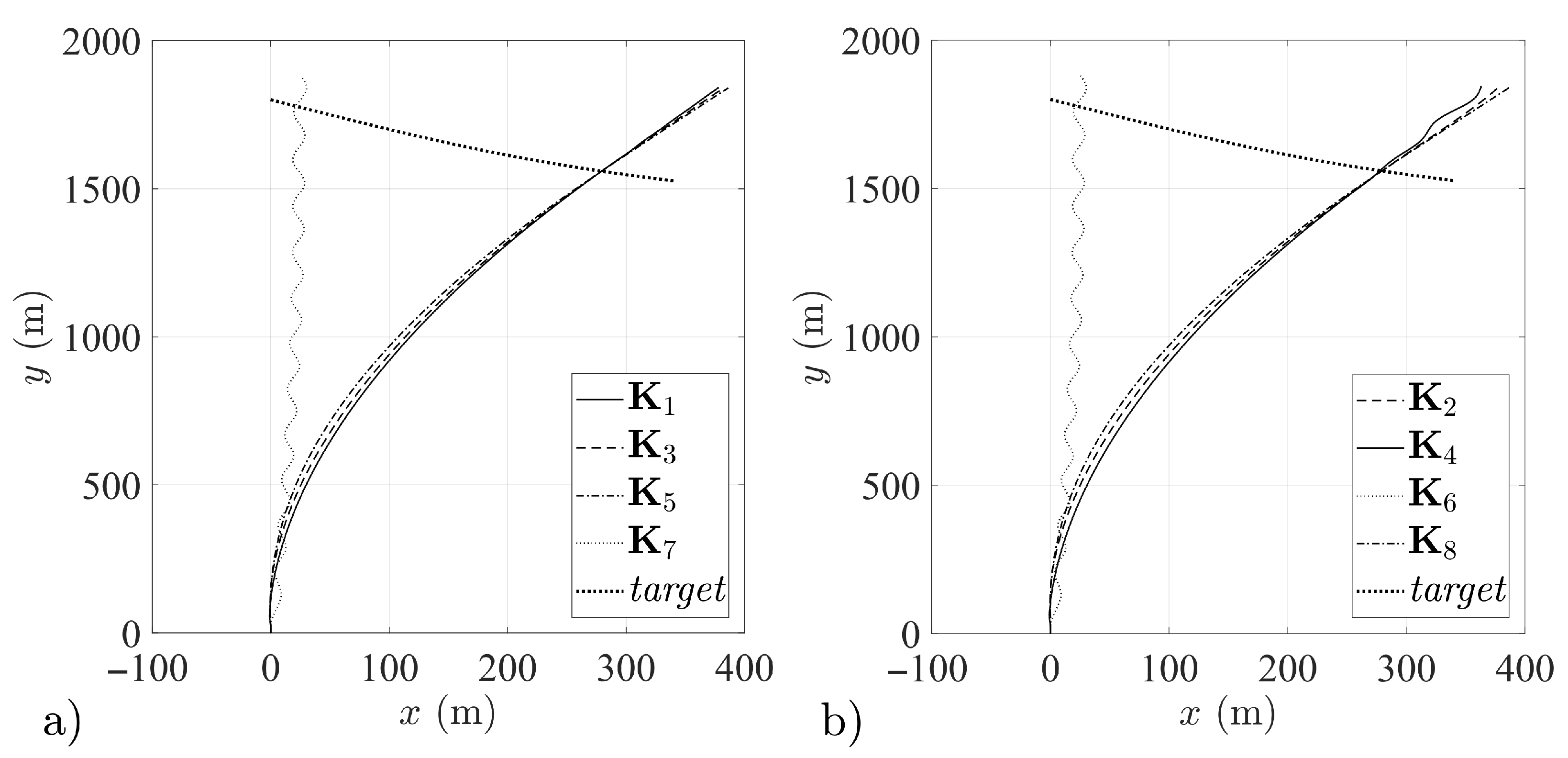
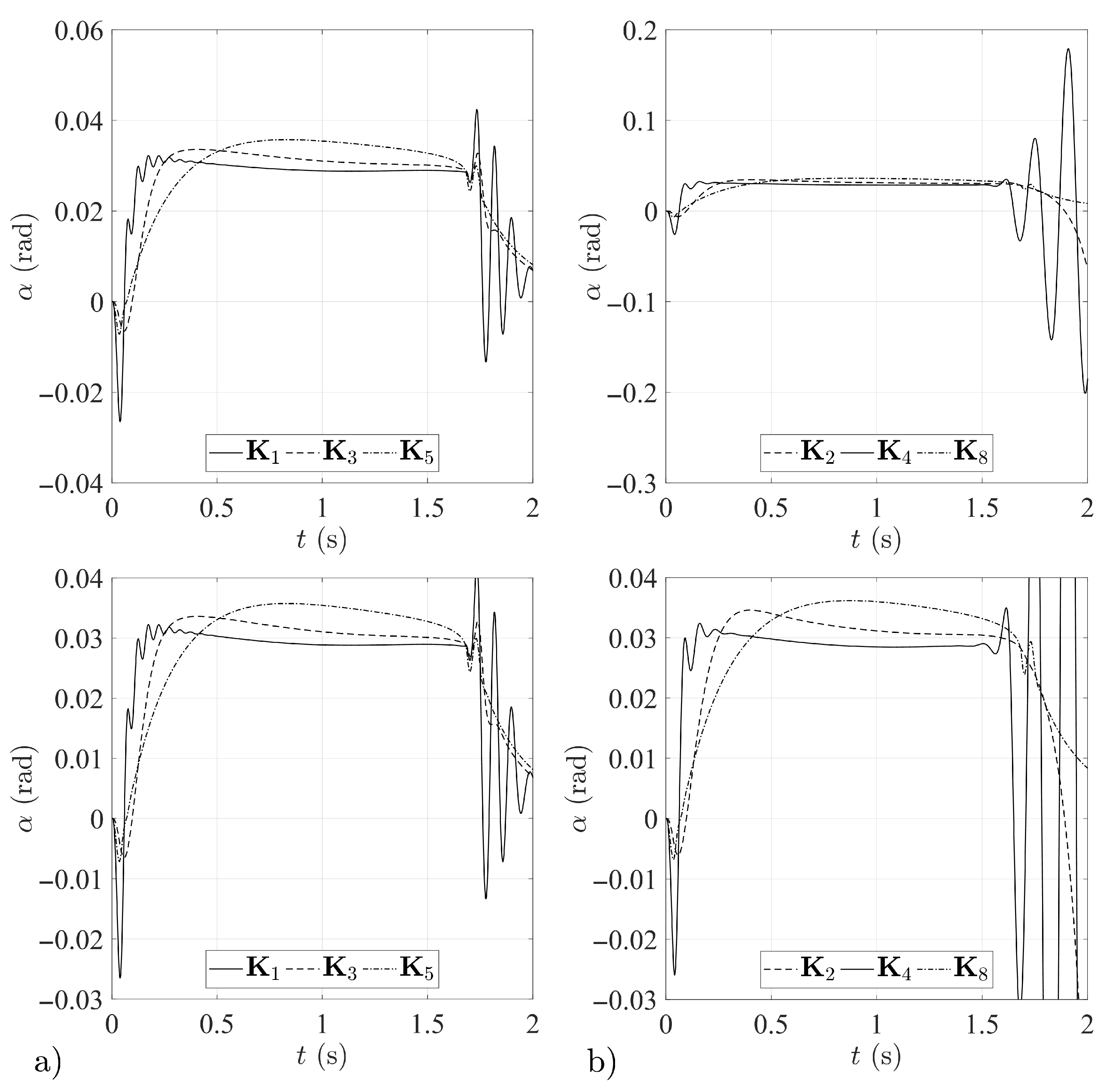
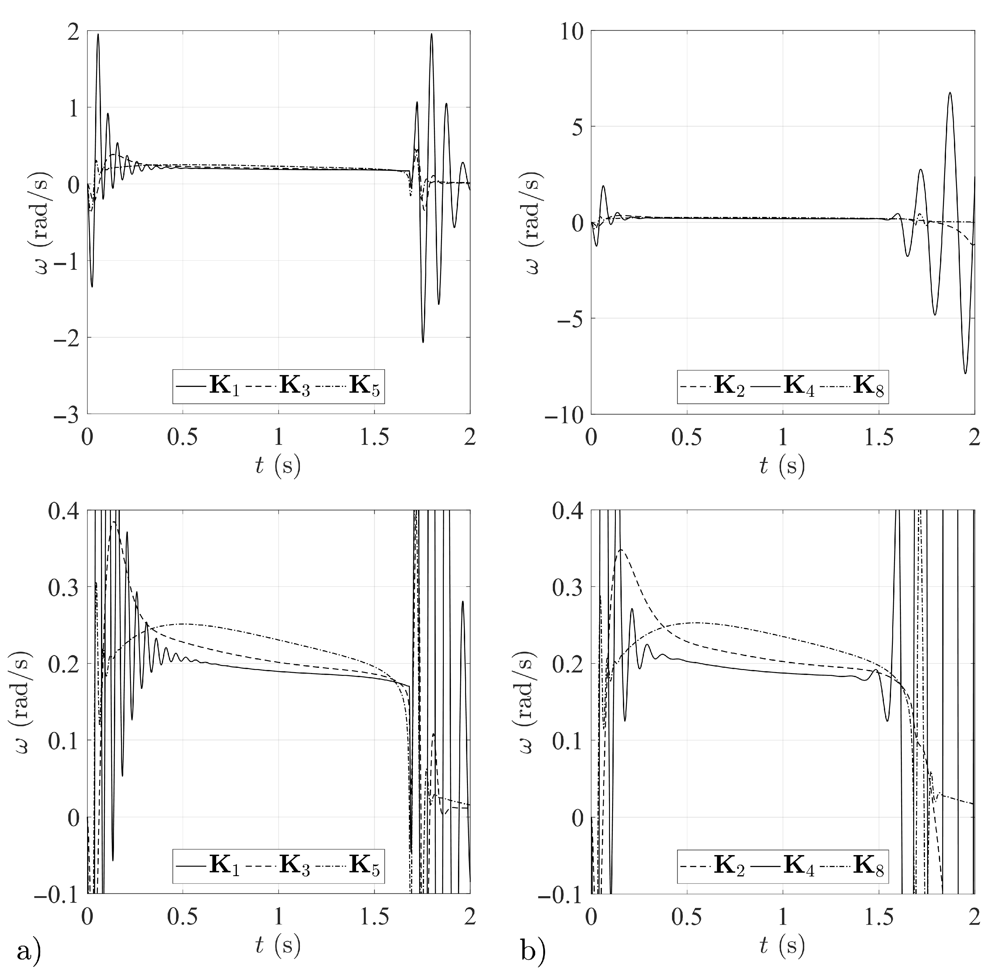
The results of the sample run test are presented in Table 2 and Figure 14, Figure 15, Figure 16, Figure 17 and Figure 18. The values of missile airframe normal acceleration a, angular rate , and angle of attack given in Table 2 are compared for the time instant .
The following conclusions can be drawn based on the simulation results.
Although in Section 2.4 values were indicated for the tuning parameter , for which the gain matrices and ought potentially to provide limited stability for the missile airframe, it was shown in the simulation tests that the proposed forms of and do not ensure the required properties of the stabilization system within the entire guidance loop (Figure 14). For this reason, these solutions were excluded from further considerations.
In the case of the gain matrices and , tests confirmed the oscillations predicted in Section 2.4, which appeared in the initial phase of guidance towards an aerial target. Over the time of the simulation the oscillations are suppressed (Figure 15, Figure 16, Figure 17 and Figure 18), but the fact of their occurrence is an unfavorable phenomenon and excludes the matrices and from the set of desired solutions. This is an interesting observation, leading to the conclusion that it is not appropriate to design individual elements of the system while neglecting properties of the guidance loop as a whole.
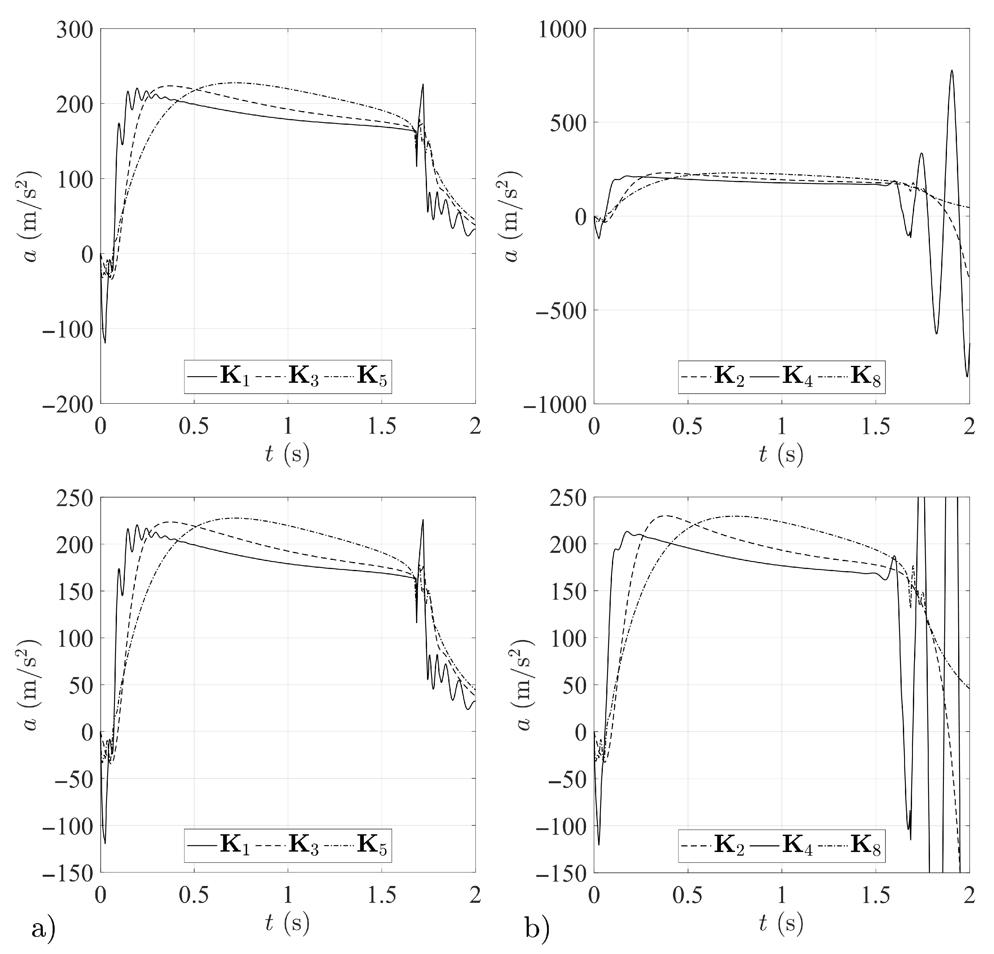
It should be noted, however, that in the case under consideration the presence of these oscillations, in spite of the increase in the value of the index , did not have a significant impact on miss distances (cf. Table 2). Moreover, missiles 1 and 4 attained the smallest instantaneous values of angle of attack (Figure 15) and normal acceleration (Figure 16) among all of the cases considered.
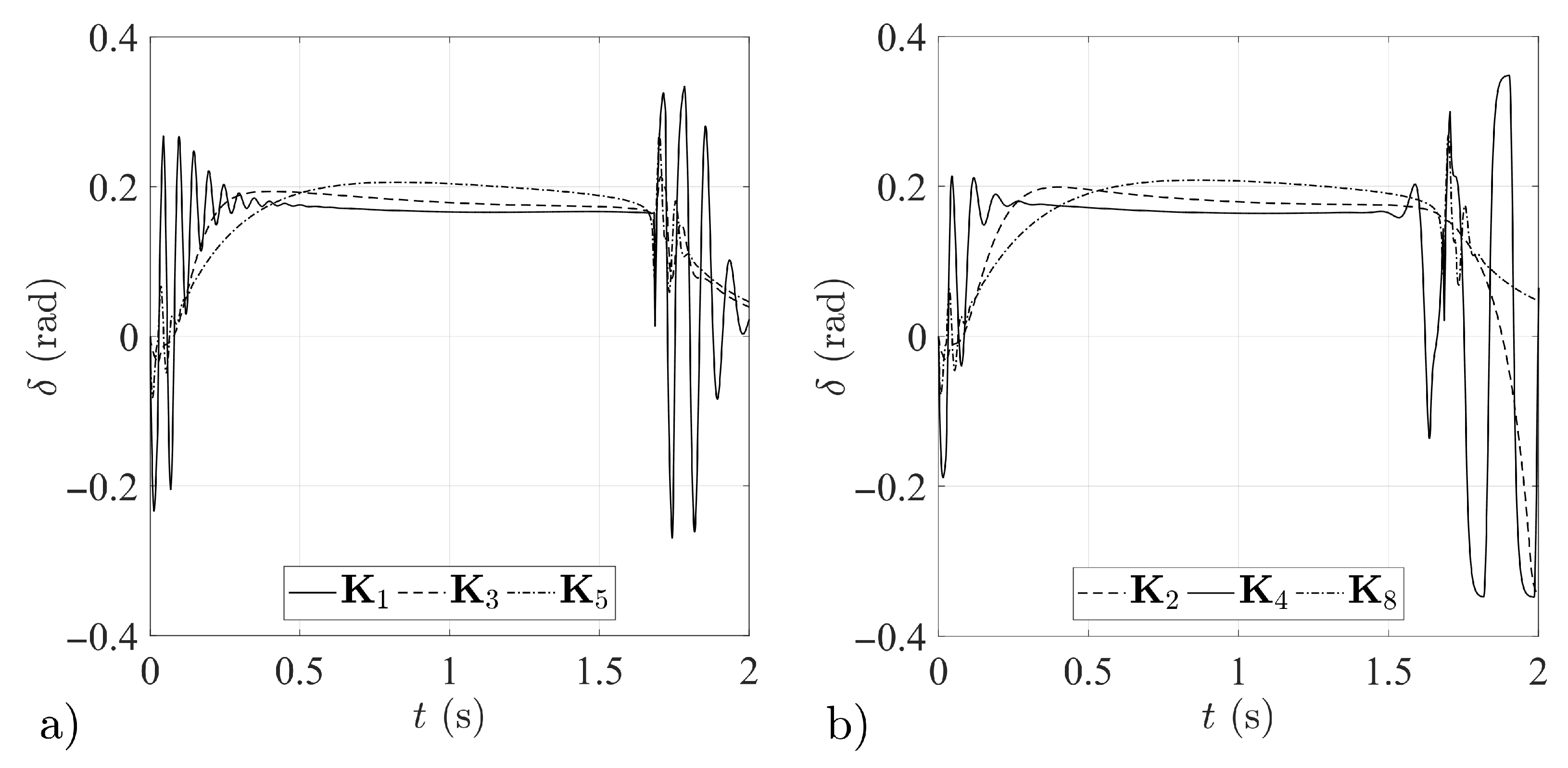
The gain matrices , , and ensure the correct operation of the airframe stabilizing loop. They correctly perform the task of regulation within the entire guidance loop. It may be noted here that the solution pair – produces greater inertia of operation than the pair –. This manifested in the higher values of the angular rates (Figure 17), angles of attack (Figure 15) and normal accelerations (Figure 16) attained by missiles 5 and 8. In this way, their regulation systems attempt to make up for the initial losses related to the delayed time of response to the input signal. Finally, however, in the case of all four missiles (numbers 2, 3, 5 and 8) the same values were obtained for the miss distances and guidance times, although the values indicate the slight superiority of missiles 2 and 3.
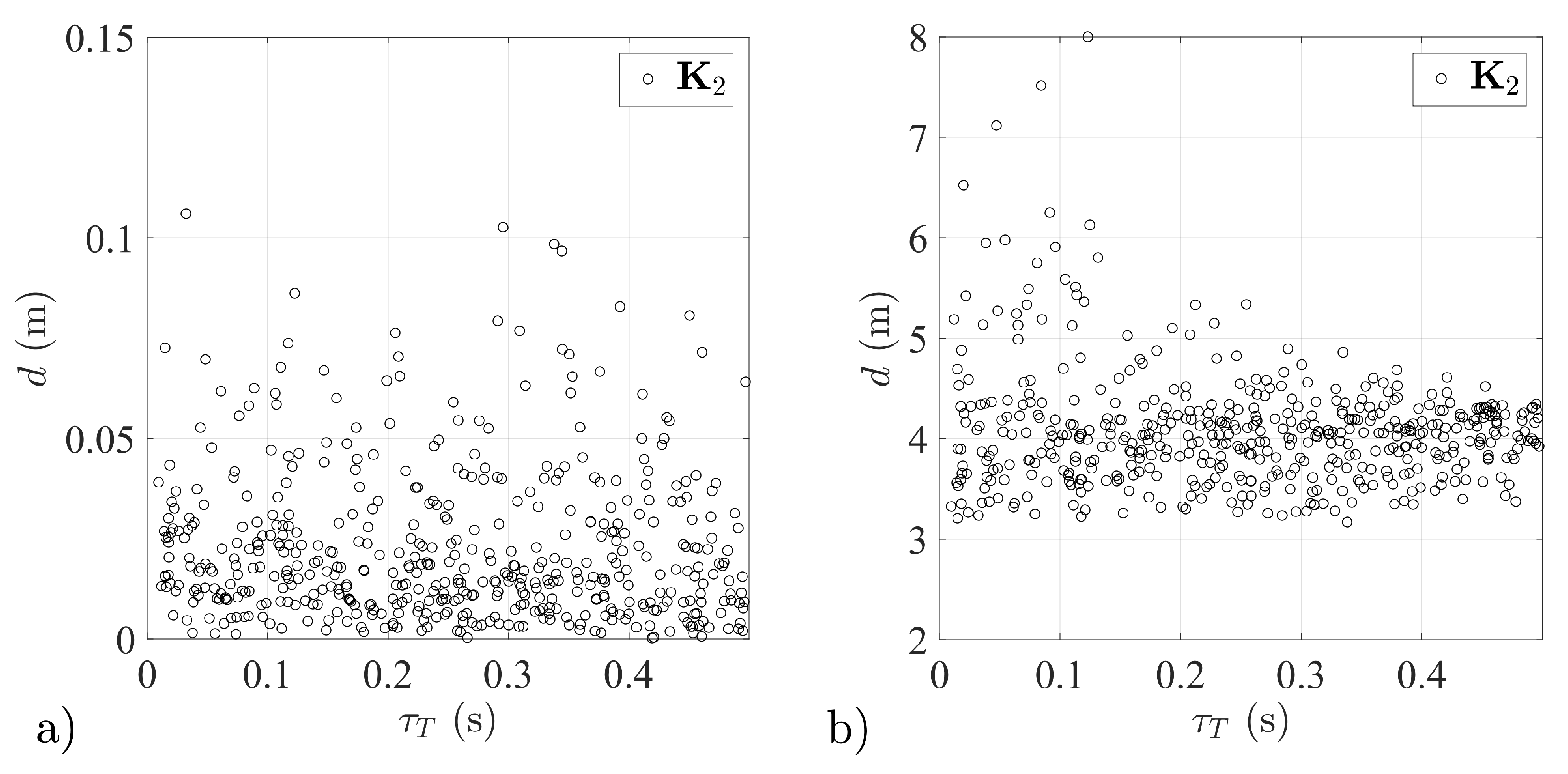
3.2. Monte Carlo Simulation Study
A Monte Carlo simulation study consisting of 500 sample runs for each missile model was carried out. In these simulations, the aerial target was located at a height of 4000 m and a distance of 1800 m from the initial position of the missiles, which was taken as described in Section 3.1. The target control commands performed square-wave evasive maneuvers in the pitch and yaw planes with a period of and a phase of relative to t = 0. For each test case, the random variables were distributed uniformly and chosen to be: time constant = (0.01 ÷ 0.5) s, velocity = (220 ÷ 340) m/s, initial pitch angle = rad and initial course angle = rad of the aerial target.
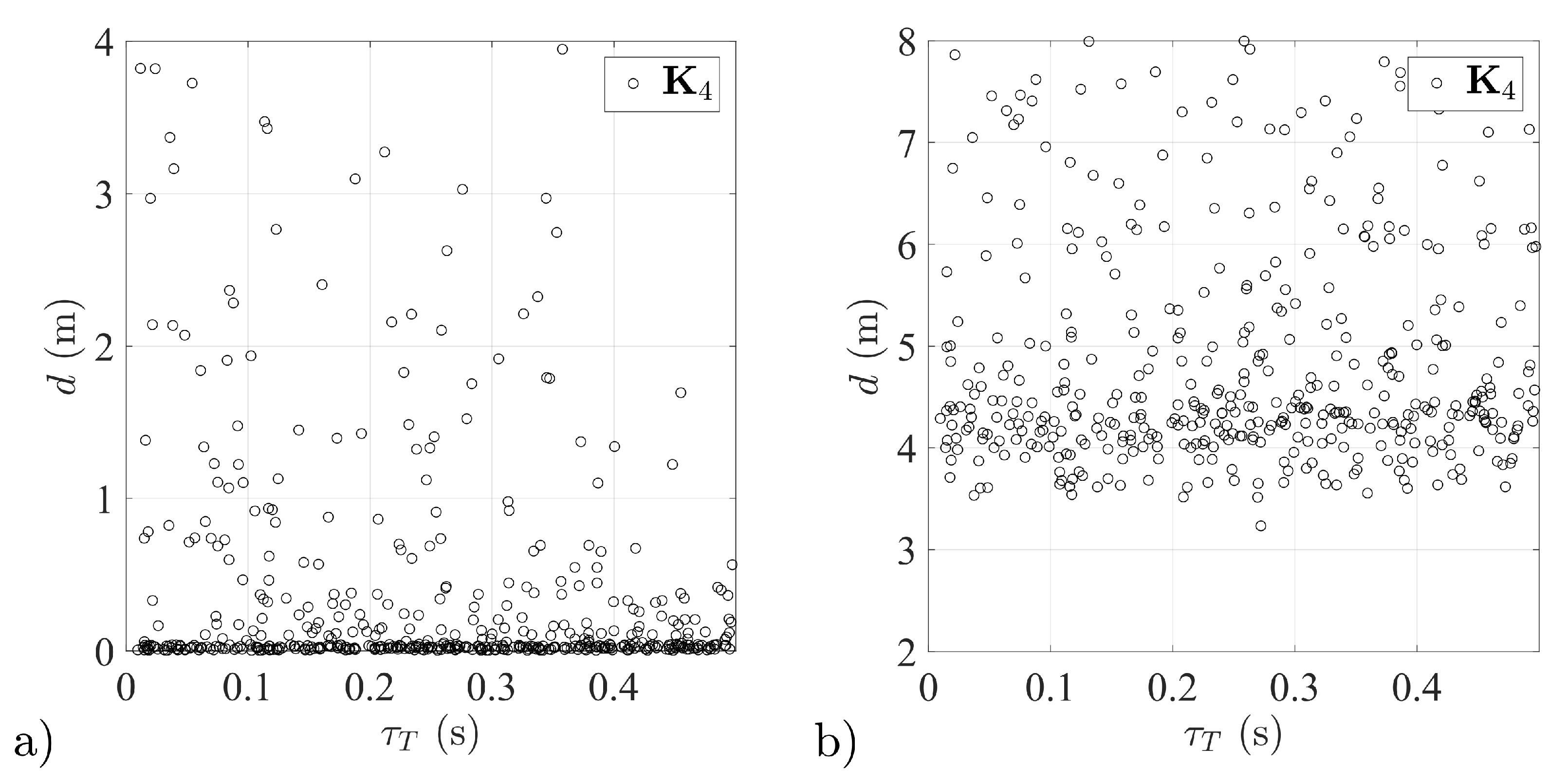
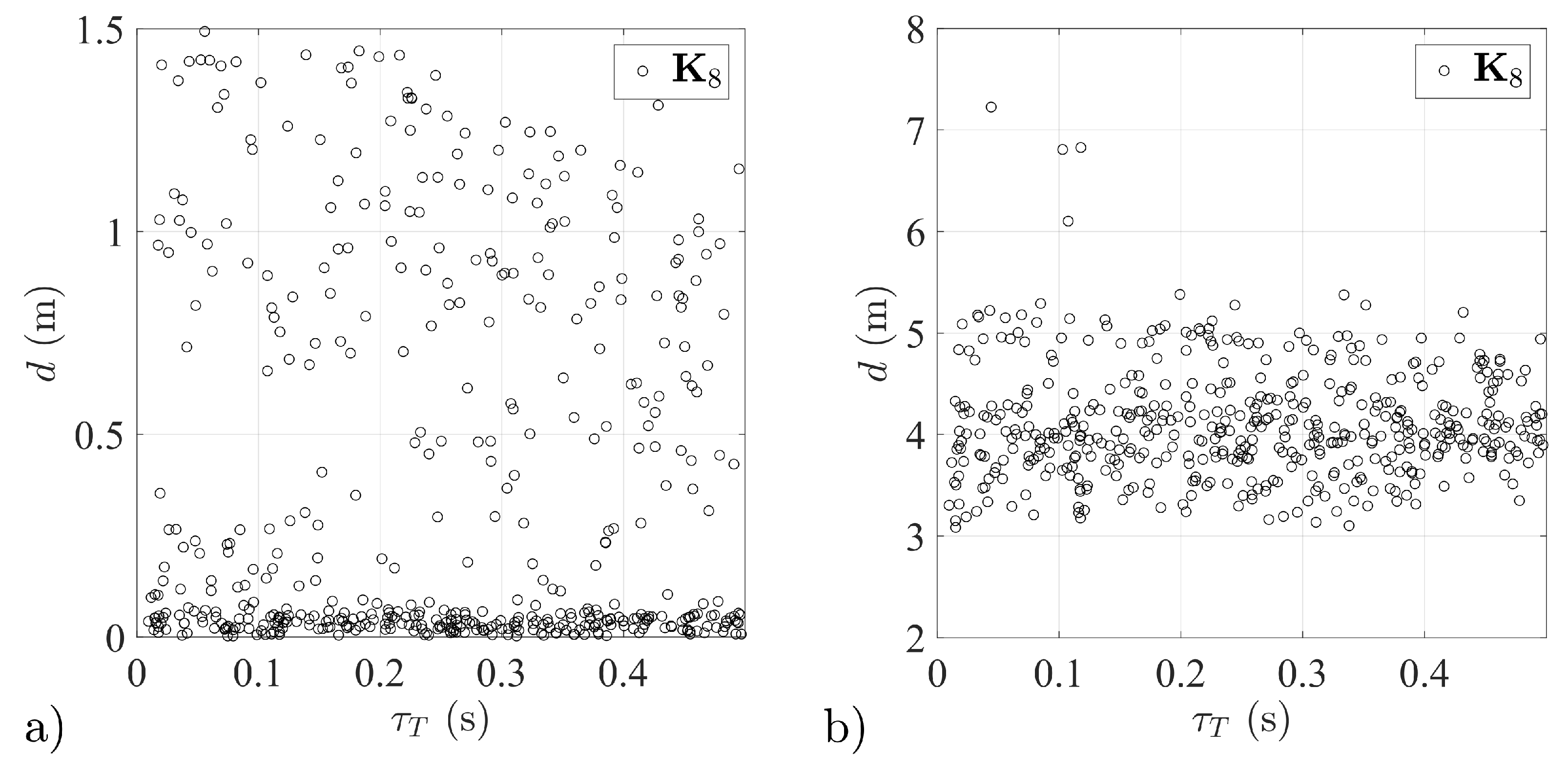
The results of the Monte Carlo simulation study are presented in Figure 19, Figure 20, Figure 21, Figure 22, Figure 23 and Figure 24. Figure 19a, Figure 20a, Figure 21a, Figure 22a, Figure 23a and Figure 24a correspond to the results of the simulation in which the proposed stabilization system was treated separately and tested in isolated conditions, where only the phenomena connected with the missile airframe dynamics were taken into account, i.e., for , and .
Figure 19b, Figure 20b, Figure 21b, Figure 22b, Figure 23b and Figure 24b correspond to the numerical simulation results achieved for the stabilization system tested as a part of the whole guidance loop. The remaining elements of the guidance loop were selected as typical and were not optimized in any way due to the final miss distance or time-to-go. Mean values of guidance results for missiles 1–5 and 8 are given in Table 3 and Table 4. For comparison, the simulation results obtained for the unstabilized airframe (missile 9) are presented, for which only the basic condition of static stability was met (the center of pressure was located behind the center of mass); cf. Figure 25, Table 3 and Table 4.
The absolute rotation angle for a Monte Carlo simulation study was taken as
where and are the missile airframe angular rates in the pitch and yaw planes (rad/s), respectively.
The following conclusions can be drawn based on the simulation results.
The greatest effectiveness of the guidance processes was obtained, in line with expectations, for missile number 3, with a stabilization system configured based on the gain matrix . It should be noted that in the case under consideration, not only was the smallest mean miss distance obtained (cf. Table 3 and Table 4) but the scatter of miss distances around the mean value was also the smallest. Moreover, this scatter tends to decrease with increasing values of the time constant characterizing the aerial target dynamics (Figure 21b).
In line with prior expectations, missile number 2, with a stabilization system based on matrix , exhibited reduced effectiveness in the case of guidance to aerial targets with a short time constant (for > 0.4 s the results are analogous to those for missile number 3; compare Figure 20 and Figure 21). This led to an increase in the mean miss distance.
Surprisingly high effectiveness was achieved in the case of missile number 1, stabilized by means of a system with matrix (Figure 19). In spite of the imperfections of this solution as outlined in Section 3.1, the system enabled the execution of guidance processes to an aerial target with an effectiveness equal to that of the system using matrix (compare Figure 19 and Figure 21). The following proved to be key factors in the case of missile number 1: rapid reaction of the system to a dynamically changing combat situation, and the ability to suppress undesired oscillations effectively.
The stabilization systems configured based on matrices and had higher mean miss distances than those based on matrices and . In the case of missiles 5 and 8, as for missiles 1, 2 and 3, a reduction was observed in the scatter of the miss distances around the mean value as the time constant increased (Figure 23 and Figure 24).
The solution using the gain matrix is to be rejected (cf. Figure 22).
It can be seen that for each of tested systems the miss distance was reduced by an order of magnitude with a radical reduction of the airframe rotation. It must be highlighted that the proposed airframe stabilization system is just a part of the autopilot and is not able to reduce the miss distance to zero. Its main task is to protect the on-board seeker before unexpected and rapid dynamic changes, which exert a negative influence on the target-tracking process. The non-zero miss distances observed in Figure 19b, Figure 20b, Figure 21b, Figure 22b, Figure 23b and Figure 24b can be explained by the fact that there are inertial components in the assumed guidance loop, e.g., from the seeker drives and actuators. Moreover, the simplest version of the proportional navigation method is used. The missiles are not guided to an overtaken point, so there are always lags behind the indications, which are evident in the case of maneuvering targets. A zero miss distance in this situation would only be achieved were the angular rate of the LOS equal to zero.
4. Conclusions
This paper has described the use of an adaptive linear-quadratic regulator to stabilize the static and dynamic characteristics of the airframe of a canard-controlled anti-aircraft missile. A procedure to determine analytically the entries of the feedback-loop gain matrix was outlined and a novel method of LQR tuning via single parameter was proposed and tested. The main effort was directed towards describing a procedure for selecting appropriate values of parameter for the designed airframe stabilization system, and presenting the results of the simulation tests. It was observed moreover, that the solutions obtained are symmetric pairs, and that the tuning parameter proposed for the designed adaptive linear-quadratic regulator enables the selection of suitable parameters for the airframe stabilizing loop for the majority of the analytical solutions of the considered matrix, the Riccati equation.
The results confirm that the analytical methods initially applied in [7,8] are correct. Likewise, they confirm the implication that the solutions found to the equations should display symmetry. In the case of six of the eight analytical solutions, it was possible to find values of the tuning parameter for which the system with a linear-quadratic regulator effectively performs the task of stabilizing the missile airframe. It should be noted, however, that not all of these solutions also provide effective guidance of the missile to an aerial target. Rather, this is a result of the properties of the guidance loop as a whole.
As mentioned at the beginning of the paper, in the aerospace field, for the applications of the LQR, the and matrices are usually determined based on Bryson principle (or modified, e.g., time-varying Bryson) or “trial and error” methods. The main problem connecting all of these is the need to define the values to find the solution of the feedback gain matrix . In the proposed concept, a basic formula of feedback loop gain matrix equations (without defining parameter , or—more precisely from the point of view of this paper—for tuning parameter = 1 in covert form) for the time-varying linear-quadratic stabilization system eliminates the need to choose values at all, as was shown in [7]. However, the approach proposed in [7] does not use all the available pairs of equations (i.e., potential solutions) describing the required operation of the stabilization system. In previous works [7,8], these pairs of equations, which give unstable solutions (with positive feedback) or which lead to inappropriate system response quality, were rejected. Here, by introducing a single tuning parameter into the equations describing the entries of gain matrix , all of the analytical solutions can be examined and fully exploited against assumed requirements.
Obtaining an analytical solution for an LQR with a single tuning parameter is very attractive from a practical (applicational) point of view. First of all, the basic form of an adaptive controller is obtained naturally. Secondly, the tuning procedure is reduced to the selection of one parameter instead of the whole matrix. The disadvantage of the proposed method is that the condition for its application is to find an analytical solution of the controller, which in general cases is difficult or impossible, e.g., because of obtaining systems of equations in entangled forms. For this reason, the discussed concept may constitute a solution for some specific control systems (those for which it is possible to find a solution in analytical form), but it cannot be treated as a universal method of designing LQR controllers.
The proposed method could be useful, e.g., when upgrading anti-aircraft missile systems of previous generations, enabling a significant increase in the capabilities of the missile with relatively negligible hardware and software interference. The algorithm is relatively easy to implement in practice. Since the coefficients given by Equation (8) are generally functions of missile velocity, with knowledge of the velocity profile, the entries of gain matrix can be found for successive time instants via preprocessing mode and then tabulated or approximated by polynomial functions. Moreover, knowledge of the airframe angular rate and the angle of attack is required. The actual value of in the control plane is supplied by an angular rate gyroscope. The value of may be determined directly or indirectly: by using an on-board instrument for measuring the angle of attack or by means of Equation (10) where the actual angle of the airframe in the control plane is supplied by a free gyroscope, whereas the angle of the velocity vector is obtained by integrating, with respect to time, the ratio of the airframe acceleration in the control plane to the missile velocity module. Both approaches give rise to certain technical and implementation problems. Discussion of these issues is beyond the scope of this paper.
However, it is necessary to note the potential dangers of the proposed approach, especially from the robustness point of view. After linearization, the control action can be very sensitive to omitted high-order terms; i.e., linear systems are not stable in a Lyapunov sense. In this paper, by calculating the feedback loop gain matrix based on the time-varying parameters and tuning parameter , an adaptive-tuned linear-quadratic stabilization system design is proposed to deal with the various disturbances affecting the operation of the seeker during the missile–target engagement process. The fact that the missile airframe behaves as a natural low-pass filter gives some additional protection (the airframe bandwidth, depending on the missile class, is usually in the range from a few to several Hz). This airframe dynamics feature quite effectively removes unwanted distortions and reduces the impacts of high order terms on the guidance process. Nevertheless, under certain unfavorable conditions, the stability of the whole system could be potentially violated. Therefore, further work should take into account the development of the proposed stabilization system towards adaptive linear robust control under external disturbance effects. From this point of view, the analysis based on the attractive ellipsoid method (AEM) seems adequate to the problem under consideration, as a methodology providing robust stabilization of dynamic systems [50,51]. In this approach, use of the dynamic model of the system is not necessary. Instead, the AEM uses basic information (i.e., the number of state variables, the number of measurable outputs and the bounds of disturbances), while providing practical stability and guaranteeing that each of the possible trajectories of the closed-loop system achieves an ellipsoid of a minimal size [50]. Future work will also be aimed at searching for a solution for the system of equations, taking into account the inertia caused by fin servos and attempting to generalize the proposed solution for the case of the pitch–yaw–roll-integrated stabilization system.
Funding
I have not received external funding.
Institutional Review Board Statement
Not applicable.
Informed Consent Statement
Not applicable.
Data Availability Statement
Sample data available on request.
Conflicts of Interest
I declare no conflict of interest.
Appendix A
The transfer function due to the takes the form
The full-state feedback system does not compare the output to the reference. Instead, it compares the state vector multiplied by the gain matrix to the reference. To obtain the desired output, the reference input must be scaled:
where N is the extra gain used to scale the closed-loop transfer function. Now we have:
It can be computed that
Appendix B
For simulation purposes, the aerial target is modeled as a mass point [6,41,45,53,54,55] whose motion in space is described by the vector of parameters
where , , are the coordinates of the target’s position (m); and are the pitch and yaw angles of the target’s velocity vector (rad), respectively; is the roll angle (rad); is the modulus of the target’s velocity vector (m/s). Changes in the target’s accelerations are approximated by the first-order dynamics
where is the commanded longitudinal acceleration (m/s); and are the manoeuvre commands in the pitch and yaw plane (m/s), respectively; is the actual longitudinal acceleration (m/s); and are the actual accelerations in the pitch and yaw plane (m/s), respectively; is the time constant of the target’s dynamics (s). The manoeuvre commands are subject to limitations in the form
Changes in the target’s velocity and in the pitch and yaw angles are defined as
while the roll angle is approximated by
where g is the gravitational acceleration (m/s). The following kinematic equations for the motion of the target’s center of mass are used:
References
- Holloway, J.C.; Krstic, M. A Predictor Observer for Seeker Delay in the Missile Homing Loop. IFAC Pap. 2015, 48, 416–421. [Google Scholar] [CrossRef]
- Kaiwei, C.; Qunli, X.; Xiao, D.; Yuemin, Y. Influence of Seeker Disturbance Rejection and Radome Error on the Lyapunov Stability of Guidance Systems. Math. Probl. Eng. 2018, 2018, 1890426. [Google Scholar] [CrossRef]
- Lin, S.; Lin, D.; Wang, W. A Novel Online Estimation and Compensation Method for Strapdown Phased Array Seeker Disturbance Rejection Effect Using Extended State Kalman Filter. IEEE Access 2019, 7, 172330–172340. [Google Scholar] [CrossRef]
- Yunli, D.; Qunli, X.; Zhuomin, W. Effect of seeker disturbance rejection performance on the control system stability. In Proceedings of the 3rd International Symposium on Systems and Control in Aeronautics and Astronautics, Harbin, China, 8–10 June 2010. [Google Scholar] [CrossRef]
- Shixiang, L.; Tianyu, L.; Teng, S.; Qunli, X. Dynamic Modeling and Coupling Characteristic Analysis of Two-Axis Rate Gyro Seeker. Int. J. Aerosp. Eng. 2018, 2018, 8513684. [Google Scholar] [CrossRef] [Green Version]
- Grycewicz, H.; Mosiewicz, R.; Pietrasieński, J. Radio Control Systems, 1st ed.; Military University of Technology: Warsaw, Poland, 1984. (In Polish) [Google Scholar]
- Bużantowicz, W. A sliding mode controller design for a missile autopilot system. J. Theor. Appl. Mech. 2020, 58, 169–182. [Google Scholar] [CrossRef]
- Bużantowicz, W. A linear-quadratic stabilization system for a canard-controlled missile. In Proceedings of the 25th International Conference “Engineering Mechanics 2019”, Svratka, Czech Republic, 13–16 May 2019; pp. 73–76. [Google Scholar] [CrossRef] [Green Version]
- Åström, K.J.; Kumar, P.R. Control: A perspective. Automatica 2014, 50, 3–43. [Google Scholar] [CrossRef]
- Ogata, K. Modern Control Engineering, 5th ed.; Prentice Hall: New York, NY, USA, 2010. [Google Scholar]
- Alameri, S.; Lazic, D.; Ristanovic, M. A Comparative Study of PID, PID with Tracking, and FPID Controller for Missile Canard with an Optimized Genetic Tuning Method Using Simscape Modelling. Teh. Vjestn. 2018, 25 (Suppl. 2), 427–436. [Google Scholar] [CrossRef]
- Kada, B. A New Methodology to Design Sliding-PID Controllers: Application to Missile Flight Control System. IFAC Proc. Vol. 2012, 45, 673–678. [Google Scholar] [CrossRef] [Green Version]
- Kianfar, K.; Amiri, R.; Bozorgmehr, A. Designing the Non-Linear PID Controller for a Missile. In Proceedings of the 1st International Conference on Informatics and Computational Intelligence, Bandung, Indonesia, 12–14 December 2011; pp. 171–175. [Google Scholar] [CrossRef]
- Zhang, W.; Lei, J.; Shi, X.; Liang, G. Research on Robustness of Double PID Control of Supersonic Missiles. In Information Computing and Applications. ICICA 2011. Communications in Computer and Information Science; Liu, C., Chang, J., Yang, A., Eds.; Springer: Berlin/Heidelberg, Germany, 2011; Volume 244. [Google Scholar] [CrossRef]
- Aboelela, M.A.S.; Ahmed, M.F.; Dorrah, H.T. Design of aerospace control systems using fractional PID controller. J. Adv. Res. 2012, 3, 225–232. [Google Scholar] [CrossRef] [Green Version]
- Ahmed, M.F.; Dorrah, H.T. Design of gain schedule fractional PID control for nonlinear thrust vector control missile with uncertainty. Automatika 2018, 59, 357–372. [Google Scholar] [CrossRef]
- Pan, B.; Fareed, U.; Qing, W.; Tian, S. A novel fractional order PID navigation guidance law by finite time stability approach. ISA Trans. 2019, 94, 80–92. [Google Scholar] [CrossRef]
- Çimen, T. A Generic Approach to Missile Autopilot Design using State-Dependent Nonlinear Control. IFAC Proc. Vol. 2011, 44, 9587–9600. [Google Scholar] [CrossRef] [Green Version]
- Menon, P.K.; Ohlmeyer, E.J. Integrated design of agile missile guidance and autopilot systems. Control Eng. Pract. 2001, 9, 1095–1106. [Google Scholar] [CrossRef]
- Chen, J.; Xiong, Z.; Liang, Z.; Bai, C.; Yi, K.; Ren, Z. Hypersonic Vehicles Profile-Following Based on LQR Design Using Time-Varying Weighting Matrices. In Advances in Some Hypersonic Vehicles Technologies, 1st ed.; Agarwal, R.K., Ed.; IntechOpen: London, UK, 2018; pp. 133–151. [Google Scholar] [CrossRef] [Green Version]
- Nocoń, Ł.; Koruba, Z. Modified linear-quadratic regulator used for controlling anti-tank guided missile in vertical plane. J. Theor. Appl. Mech. 2020, 58, 723–732. [Google Scholar] [CrossRef]
- Park, J.; Kim, Y.; Kim, J.H. Integrated Guidance and Control Using Model Predictive Control with Flight Path Angle Prediction against Pull-Up Maneuvering Target. Sensors 2020, 20, 3143. [Google Scholar] [CrossRef] [PubMed]
- Talole, S.E.; Godbole, A.A.; Kolhe, J.P.; Phadke, S.B. Robust Roll Autopilot Design for Tactical Missiles. J. Guid. Control Dyn. 2011, 34, 107–118. [Google Scholar] [CrossRef]
- Vincent, R.V.; Economou, J.; Wall, D.G.; Cleminson, J. H∞/LQR Optimal Control for a Supersonic Air-Breathing Missile of Asymmetric Configuration. IFAC Pap. 2019, 52, 214–218. [Google Scholar] [CrossRef]
- Devan, V.; Chandar, T.S. Cascaded LQR Control for Missile Roll Autopilot. In Proceedings of the 2018 International CET Conference on Control, Communication, and Computing (IC4), Trivandrum, India, 5–7 July 2018; pp. 45–50. [Google Scholar] [CrossRef]
- Wise, K.A. A Trade Study on Missile Autopilot Design Using Optimal Control Theory. In Proceedings of the AIAA Guidance, Navigation and Control Conference and Exhibit, Hilton Head, SD, USA, 20–23 August 2007. [Google Scholar] [CrossRef]
- Çimen, T. State-Dependent Riccati Equation (SDRE) Control: A Survey. IFAC Proc. Vol. 2008, 41, 3761–3775. [Google Scholar] [CrossRef] [Green Version]
- Franklin, G.F.; Powell, D.J.; Emami-Naeini, A. Feedback Control of Dynamic Systems, 6th ed.; Pearson Education: London, UK, 2011. [Google Scholar]
- Åström, K.J.; Murray, R.M. Feedback Systems: An Introduction for Scientists and Engineers, 1st ed.; Princeton University Press: Princeton, NJ, USA, 2012. [Google Scholar]
- Deng, X.; Sun, X.; Liu, R.; Wei, W. Optimal analysis of the weighted matrices in LQR based on the differential evolution algorithm. In Proceedings of the 29th Chinese Control and Decision Conference (CCDC), Chongqing, China, 28–30 May 2017; pp. 832–836. [Google Scholar] [CrossRef]
- Dong-Qing, F. Simulation Research on the Weighting Matrix of the Optimal Linear System. J. Zhengzhou Univ. Technol. 2000, 21, 11–14. [Google Scholar]
- Li, Y.; Liu, J.; Wang, Y. Design Approach of Weighting Matrices for LQR Based on Multi-objective Evolution Algorithm. In Proceedings of the 2008 IEEE International Conference on Information and Automation, Changsha, China, 20–23 June 2008; pp. 1188–1192. [Google Scholar] [CrossRef]
- Peng, Y.; Chen, Y.Q. Optimal design of the LQR controller based on the improved shuffled frog-leaping algorithm. CAAI Trans. Intell. Syst. 2014, 9, 480–484. [Google Scholar] [CrossRef]
- Siddiq, M.K.; Cheng, F.J.; Bo, Y.W. SDRE Based Integrated Roll, Yaw and Pitch Controller Design for 122 mm Artillery Rocket. Appl. Mech. Mater. 2013, 415, 200–208. [Google Scholar] [CrossRef]
- Abdelhamid, A.M.; El-Gaafary, A. Optimal Decentralized LQR Control to Enhance Multi-Area LFC System Stability. Math. Probl. Eng. 2018, 2018, 7232915. [Google Scholar] [CrossRef] [Green Version]
- Stefanescu, R.M.; Prioroc, C.L.; Stoica, A.M. Weighting matrices determination using pole placement for tracking maneuvers. UPB Sci. Bull. Ser. D Mech. Eng. 2013, 75, 31–40. [Google Scholar]
- Siouris, G.M. Missile Guidance and Control Systems, 1st ed.; Springer: New York, NY, USA, 2004. [Google Scholar]
- Zarchan, P. Tactical and Strategic Missile Guidance, 6th ed.; AIAA: Reston, VA, USA, 2012. [Google Scholar]
- Zaikang, Q.; Defu, L. Design of Guidance and Control Systems for Tactical Missiles, 1st ed.; CRC Press: Boca Raton, FL, USA, 2020. [Google Scholar]
- Brugarolas, P.B.; Fromion, V.; Safonov, M.G. Robust switching missile autopilot. In Proceedings of the American Control Conference, Philadelphia, PA, USA, 24–26 June 1998; Volume 6, pp. 3665–3669. [Google Scholar] [CrossRef]
- Idan, M.; Shima, T.; Golan, O.M. Integrated Sliding Mode Autopilot-Guidance for Dual Control Missiles. J. Guid. Control Dyn. 2007, 30, 1081–1089. [Google Scholar] [CrossRef]
- Lee, H.C.; Choi, J.W.; Song, T.L.; Song, C.H. Agile Missile Autopilot Design via Time-Varying Eigenvalue Assigment. In Proceedings of the 8th International Conference on Control, Automation, Robotics and Vision, Kunming, China, 6–9 December 2004; pp. 1832–1837. [Google Scholar] [CrossRef]
- McLain, T.W.; Beard, R.W. Nonlinear Robust Missile Autopilot Design Using Successive Galerkin Approximation. In Proceedings of the AIAA Guidance, Navigation, and Control Conference and Exhibit, Portland, OR, USA, 9–11 August 1999; pp. 384–391. [Google Scholar] [CrossRef] [Green Version]
- Shamma, J.S.; Cloutier, J.R. Gain-Sheduled Missile Autopilot Design Using Linear Parameter Varying Transformations. J. Guid. Control Dyn. 1993, 16, 256–263. [Google Scholar] [CrossRef]
- Shima, T.; Idan, M.; Golan, O.M. Sliding-Mode Control for Integrated Missile Autopilot Guidance. J. Guid. Control Dyn. 2006, 29, 250–260. [Google Scholar] [CrossRef]
- Zhao, Z.; Jun, H. A High Gain Integral Dynamic Compensation Method for Nonlinear Missile Control. IFAC Proc. Vol. 2011, 44, 2048–2053. [Google Scholar] [CrossRef] [Green Version]
- Cronvich, L.L. Missile Aerodynamics. Johns Hopkins APL Tech. Dig. 1983, 4, 175–186. [Google Scholar]
- Kurov, V.D.; Dolzhansky, J.M. Principles Behind the Solid-Propellant Rocket Design, 1st ed.; Publishing House of Ministry of National Defense: Warsaw, Poland, 1964. (In Polish) [Google Scholar]
- Moore, F. Approximate Methods for Weapon Aerodynamics, 1st ed.; Progress in Astronautics and Aeronautics; AIAA: Reston, VT, USA, 2000; Volume 186. [Google Scholar] [CrossRef]
- Ordaz, P.; Poznyak, A. The Furuta’s Pendulum Stabilization without the Use of a Mathematical Model: Attractive Ellipsoid Method with KL-adaptation. In Proceedings of the 51st IEEE Conference on Decision and Control (CDC), Maui, HI, USA, 10–13 December 2012; pp. 7285–7290. [Google Scholar] [CrossRef]
- Ordaz, P.; Poznyak, A. Adaptive-Robust Stabilization of the Furuta’s Pendulum via Attractive Ellipsoid Method. J. Dyn. Syst. Meas. Control 2016, 138, 021005. [Google Scholar] [CrossRef]
- Franklin, G.F.; Powell, D.J.; Workman, M.L. Digital Control of Dynamic Systems, 3rd ed.; Addison-Wesley: Menlo Park, CA, USA, 1997. [Google Scholar]
- Lin, C.L.; Chen, Y.Y. Design of Fuzzy Logic Guidance Law Against High-Speed Target. J. Guid. Control Dyn. 2000, 23, 17–25. [Google Scholar] [CrossRef]
- Bużantowicz, W. Dual-control missile guidance: A simulation study. J. Theor. Appl. Mech. 2018, 56, 727–739. [Google Scholar] [CrossRef]
- Bużantowicz, W. A Method of Visualizing Velocity and Acceleration Profiles of an Air Target. Probl. Mechatronics. Armament Aviat. Saf. Eng. 2018, 9, 9–20. [Google Scholar] [CrossRef]
Figure 1.
Tuning procedure results for feedback loop gain matrix : (a) Quantity indices for different values. (b) Step responses of the airframe before and after the tuning procedure.
Figure 1.
Tuning procedure results for feedback loop gain matrix : (a) Quantity indices for different values. (b) Step responses of the airframe before and after the tuning procedure.

Figure 2.
Tuning procedure results for feedback loop gain matrix : (a) Quantity indices for different values. (b) Step responses of the airframe before and after the tuning procedure.
Figure 2.
Tuning procedure results for feedback loop gain matrix : (a) Quantity indices for different values. (b) Step responses of the airframe before and after the tuning procedure.

Figure 3.
Tuning procedure results for feedback loop gain matrix : (a) Quantity indices for different values. (b) Step responses of the airframe before and after the tuning procedure.
Figure 3.
Tuning procedure results for feedback loop gain matrix : (a) Quantity indices for different values. (b) Step responses of the airframe before and after the tuning procedure.

Figure 4.
Tuning procedure results for feedback loop gain matrix : (a) Quantity indices for different values. (b) Step responses of the airframe before and after the tuning procedure.
Figure 4.
Tuning procedure results for feedback loop gain matrix : (a) Quantity indices for different values. (b) Step responses of the airframe before and after the tuning procedure.

Figure 5.
Tuning procedure results for feedback loop gain matrix : (a) Quantity indices for different values. (b) Step responses of the airframe before and after the tuning procedure.
Figure 5.
Tuning procedure results for feedback loop gain matrix : (a) Quantity indices for different values. (b) Step responses of the airframe before and after the tuning procedure.

Figure 6.
Tuning procedure results for feedback loop gain matrix : (a) Quantity indices for different values. (b) Step responses of the airframe before and after the tuning procedure.
Figure 6.
Tuning procedure results for feedback loop gain matrix : (a) Quantity indices for different values. (b) Step responses of the airframe before and after the tuning procedure.

Figure 7.
Tuning procedure results for feedback loop gain matrix : (a) Quantity indices for different values. (b) Step responses of the airframe before and after the tuning procedure.
Figure 7.
Tuning procedure results for feedback loop gain matrix : (a) Quantity indices for different values. (b) Step responses of the airframe before and after the tuning procedure.

Figure 8.
Tuning procedure results for feedback loop gain matrix : (a) Quantity indices for different values. (b) Step responses of the airframe before and after the tuning procedure.
Figure 8.
Tuning procedure results for feedback loop gain matrix : (a) Quantity indices for different values. (b) Step responses of the airframe before and after the tuning procedure.

Figure 9.
Symmetry between quantity indices of matrices and .

Figure 10.
Symmetry between quantity indices of matrices and .

Figure 11.
Symmetry between quantity indices of matrices and .

Figure 12.
Symmetry between quantity indices of matrices and .

Figure 13.
Missile airframe: (a,b) angular rate, (c,d) angle of attack histories for different feedback loop gain matrices.
Figure 13.
Missile airframe: (a,b) angular rate, (c,d) angle of attack histories for different feedback loop gain matrices.

Figure 14.
Missile and target trajectories for: (a) missiles 1, 3, 5 and 7, (b) missiles 2, 4, 6 and 8.
Figure 14.
Missile and target trajectories for: (a) missiles 1, 3, 5 and 7, (b) missiles 2, 4, 6 and 8.

Figure 15.
Angle of attack histories for: (a) missiles 1, 3 and 5, (b) missiles 2, 4 and 8.

Figure 16.
Airframe normal acceleration histories for: (a) missiles 1, 3 and 5, (b) missiles 2, 4 and 8.
Figure 16.
Airframe normal acceleration histories for: (a) missiles 1, 3 and 5, (b) missiles 2, 4 and 8.

Figure 17.
Canard-fin deflection histories for: (a) missiles 1, 3 and 5; (b) missiles 2, 4 and 8.

Figure 18.
Airframe angular rate histories for: (a) missiles 1, 3 and 5; (b) missiles 2, 4 and 8.

Figure 19.
Miss distance distributions for different aerial target dynamics—stabilization system with matrix tested: (a) in isolated conditions, (b) as a part of a guidance loop.
Figure 19.
Miss distance distributions for different aerial target dynamics—stabilization system with matrix tested: (a) in isolated conditions, (b) as a part of a guidance loop.

Figure 20.
Miss distance distributions for different aerial target dynamics—stabilization system with matrix tested: (a) in isolated conditions, (b) as a part of a guidance loop.
Figure 20.
Miss distance distributions for different aerial target dynamics—stabilization system with matrix tested: (a) in isolated conditions, (b) as a part of a guidance loop.

Figure 21.
Miss distance distributions for different aerial target dynamics—stabilization system with matrix tested: (a) in isolated conditions, (b) as a part of a guidance loop.
Figure 21.
Miss distance distributions for different aerial target dynamics—stabilization system with matrix tested: (a) in isolated conditions, (b) as a part of a guidance loop.

Figure 22.
Miss distance distributions for different aerial target dynamics—stabilization system with matrix tested: (a) in isolated conditions, (b) as a part of a guidance loop.
Figure 22.
Miss distance distributions for different aerial target dynamics—stabilization system with matrix tested: (a) in isolated conditions, (b) as a part of a guidance loop.

Figure 23.
Miss distance distributions for different aerial target dynamics—stabilization system with matrix tested: (a) in isolated conditions, (b) as a part of a guidance loop.
Figure 23.
Miss distance distributions for different aerial target dynamics—stabilization system with matrix tested: (a) in isolated conditions, (b) as a part of a guidance loop.

Figure 24.
Miss distance distributions for different aerial target dynamics—stabilization system with matrix tested: (a) in isolated conditions, (b) as a part of a guidance loop.
Figure 24.
Miss distance distributions for different aerial target dynamics—stabilization system with matrix tested: (a) in isolated conditions, (b) as a part of a guidance loop.

Figure 25.
Miss distance distributions for different aerial target dynamics—unstabilized airframe tested: (a) in isolated conditions, (b) as a part of guidance loop.
Figure 25.
Miss distance distributions for different aerial target dynamics—unstabilized airframe tested: (a) in isolated conditions, (b) as a part of guidance loop.


Table 1.
Symmetry between gain matrices and tuning parameter values.
| Gain | Tuning Parameter | Axis of Symmetry | Tuning Parameter | Gain | ||
|---|---|---|---|---|---|---|
| Matrix | Matrix | |||||
| −5.060 | −5.015 | −0.045 | 5.015 | 4.970 | ||
| 0.940 | −0.310 | 1.250 | 0.310 | 1.560 | ||
| −9.190 | −8.455 | −0.735 | 8.455 | 7.720 | ||
| −6.210 | −7.000 | 0.790 | 7.000 | 7.790 |
Table 2.
Simulation results for the sample run test.
| Missile | Gain | d | |||||
|---|---|---|---|---|---|---|---|
| Number | Matrix | (s) | (m) | (m/s) | (rad/s) | (rad) | (rad) |
| 1 | 1.68 | 3.51 | 163.28 | 0.170 | 0.029 | 0.4009 | |
| 2 | 1.68 | 3.51 | 161.05 | 0.136 | 0.029 | 0.3608 | |
| 3 | 1.68 | 3.51 | 164.26 | 0.154 | 0.029 | 0.3615 | |
| 4 | 1.68 | 4.22 | −102.01 | −0.459 | −0.032 | 0.4604 | |
| 5 | 1.68 | 3.51 | 159.16 | 0.090 | 0.029 | 0.3744 | |
| 6 | 1.61 | 242.53 | ― | ― | ― | 6.6262 | |
| 7 | 1.61 | 242.48 | ― | ― | ― | 6.6212 | |
| 8 | 1.68 | 3.51 | 155.68 | 0.067 | 0.029 | 0.3751 |
Table 3.
Mean values of guidance results (for isolated conditions).
| Missile Number | Gain Matrix | |||
|---|---|---|---|---|
| (s) | (m) | (rad) | ||
| 1 | 1.5536 | 0.0269 | 0.8779 | |
| 2 | 1.5442 | 0.0324 | 0.8034 | |
| 3 | 1.5536 | 0.0259 | 0.8046 | |
| 4 | 1.5535 | 0.6617 | 1.0073 | |
| 5 | 1.5544 | 0.2885 | 0.8369 | |
| 8 | 1.5543 | 0.4090 | 0.8334 | |
| 9 | unstabilized | 1.5536 | 5.7028 | 6.3302 |
Table 4.
Mean values of guidance results (for the whole guidance loop).
| Missile Number | Gain Matrix | |||
|---|---|---|---|---|
| (s) | (m) | (rad) | ||
| 1 | 1.5575 | 3.87 | 0.7433 | |
| 2 | 1.5580 | 4.10 | 0.6692 | |
| 3 | 1.5580 | 3.86 | 0.6705 | |
| 4 | 1.5576 | 5.44 | 0.8537 | |
| 5 | 1.5585 | 4.07 | 0.6946 | |
| 8 | 1.5553 | 4.17 | 0.6945 | |
| 9 | unstabilized | 1.5609 | 23.99 | 5.3195 |
Publisher’s Note: MDPI stays neutral with regard to jurisdictional claims in published maps and institutional affiliations. |
© 2021 by the author. Licensee MDPI, Basel, Switzerland. This article is an open access article distributed under the terms and conditions of the Creative Commons Attribution (CC BY) license (http://creativecommons.org/licenses/by/4.0/).
Share and Cite
MDPI and ACS Style
Bużantowicz, W. Tuning of a Linear-Quadratic Stabilization System for an Anti-Aircraft Missile. Aerospace 2021, 8, 48. https://0-doi-org.brum.beds.ac.uk/10.3390/aerospace8020048
AMA Style
Bużantowicz W. Tuning of a Linear-Quadratic Stabilization System for an Anti-Aircraft Missile. Aerospace. 2021; 8(2):48. https://0-doi-org.brum.beds.ac.uk/10.3390/aerospace8020048
Chicago/Turabian StyleBużantowicz, Witold. 2021. "Tuning of a Linear-Quadratic Stabilization System for an Anti-Aircraft Missile" Aerospace 8, no. 2: 48. https://0-doi-org.brum.beds.ac.uk/10.3390/aerospace8020048
Note that from the first issue of 2016, this journal uses article numbers instead of page numbers. See further details here.