
Methods of Identifying Correlated Model Parameters with Noise in Prognostics


Department of Mechanical and Aerospace Engineering, University of Florida, Gainesville, FL 32611, USA
*
Author to whom correspondence should be addressed.
Aerospace 2021, 8(5), 129; https://0-doi-org.brum.beds.ac.uk/10.3390/aerospace8050129
Submission received: 14 March 2021
/
Revised: 29 April 2021
/
Accepted: 1 May 2021
/
Published: 5 May 2021
(This article belongs to the Special Issue Fault Detection and Prognostics in Aerospace Engineering)
Abstract
:In physics-based prognostics, model parameters are estimated by minimizing the error or maximizing the likelihood between model predictions and measured data. When multiple model parameters are strongly correlated, it is challenging to identify individual parameters by measuring degradation data, especially when the data have noise. This paper first presents various correlations that occur during the process of model parameter estimation and then introduces two methods of identifying the accurate values of individual parameters when they are strongly correlated. The first method can be applied when the correlation relationship evolves as damage grows, while the second method can be applied when the operating (loading) conditions change. Starting from manufactured data using the true parameters, the accuracy of identified parameters is compared with various levels of noise. It turned out that the proposed method can identify the accurate values of model parameters even with a relatively large level of noise. In terms of the marginal distribution, the standard deviation of a model parameter is reduced from 0.125 to 0.03 when different damage states are used. When the loading conditions change, the uncertainty is reduced from 0.3 to 0.05. Both are considered as a significant improvement.
1. Introduction
Aircraft structures are designed based on the damage-tolerance concept, where flaws can exist in any structure and such flaws propagate with usage. A maintenance program will result in the detection and repair of damage, corrosion and fatigue cracking before such damage threatens the safety of the system. Structural maintenance of aircraft is currently based on scheduled maintenance, which accounts for more than 27% of the lifecycle cost of an aircraft [1]. There are ongoing research efforts to reduce the maintenance cost by utilizing condition-based maintenance where the health status of the system is continuously monitored, and maintenance is requested when the safety of the system is threatened [2].
Structural health monitoring (SHM) [3,4,5] is the process of identifying damage and evaluating the safety of a system based on online and/or offline data. It uses an array of sensors to obtain measurement data that are directly or indirectly related to damage. The statistical analysis of these measurements can help predict the future state of the system and thus improve the safety of the system. SHM can be found in a wide variety of applications such as bridges and dams [6], buildings [7], stadiums, platforms, airframes [8], power plants [9], etc. Prognostics is an extension of SHM, which is the process of estimating the time beyond which a system can no longer function to meet desired performances [10]. The time, in terms of cycles/hours, remaining to run the system before failure is called the remaining useful life (RUL).
There are two types of prognostics methods: data-driven and physics-based approaches [11]. The data-driven approaches [12] are advantageous when many training data are available for a complex system, while the physics-based approaches [13,14] are good when a physical model of damage degradation is available. In this paper, the physics-based approach is used for prognostics, where a well-defined physics model is assumed to be available to represent the progression of degradation, and measurement data are used to estimate the model parameters, from which the RUL can be predicted.
Identifying model parameters is the key step in the prognostics using physics-based approaches [15] because, with the identified parameters, the RUL can easily be calculated by propagating the degradation model to the future. In addition to operating conditions and model-form errors, it is critically important to identify uncertainty in the parameters, as they are directly related to the uncertainty in the RUL. In addition, when multiple parameters are involved, it is important to identify the correlation between them. Correlation occurs when the combinations of more than one parameter can represent the same physical phenomenon. For example, in Paris crack growth model, different combinations of two model parameters can yield the same crack growth rate [16]. This often happened because a single physical quantity is measured, while multiple parameters influence the quantity.
Model parameter identification is equivalent to a curve-fitting process where the errors between model predictions and measured data are minimized using linear/nonlinear regression [10]. Recently, statistical estimation methods have become popular to consider the uncertainty in future degradation [17]. Many of the statistical approaches have their theoretical foundation on the Bayesian inference, where the observed data can improve the information on the current model parameters. In the case of statistical approaches, the maximum likelihood estimation is often used to identify the probability distribution of model parameters [18]. In Bayesian inference, the joint probability density function (PDF) of model parameters is updated from its prior PDF to the posterior PDF. The posterior PDF shows the level of knowledge in the unknown parameters based on the observed data.
In general, correlation in statistics measures the similarity in trend between two or more random variables. In the regime of epistemic uncertainty of model parameters, two parameters are considered to be correlated when multiple combinations of them can predict the same degradation state. Since the predicted value is the same, it is inherently difficult to identify individual values of parameters. Instead, a relationship between them can be obtained. If the marginal PDF of individual parameters is used, the RUL prediction can significantly be different from the true one. Therefore, it is important to identify the correlation structure between degradation parameters. Li and Vu [19] presented non-identifiability problems of biology model parameters in nonlinear dynamic models due to correlations between parameters. Santos and Pinto [20] showed that when a variable correlation is unknown, the simultaneous estimation of model parameters and variable correlation may lead to meaningless parameter estimates and parameter uncertainties. In statistical approaches, Matzke et al. [21] used Bayesian inference to quantify the correlation uncertainty in the presence of measurement error. Most literature on correlation focuses on identifying the correlation structure, not the value of parameters.
An important contribution of the present work is related to the fact that the number of unknown model parameters is normally larger than that of the measurement data types. Normally a single type of degradation data is measured while multiple model parameters need to be estimated. In addition, these parameters are often strongly correlated. In such a situation, it is difficult, if not impossible, to identify the accurate model parameters. An et al. [16] showed that even if the accurate model parameters may not be identified, the correlation relationship can still be used to predict the RUL accurately. However, it is often necessary to identify accurate model parameters in order to use them under different operating conditions or to use them in different systems.
The objective of this paper is to present various types of correlations that occur during model parameter estimation and then introduce two ways of identifying degradation parameters even if the correlation between them is strong. The idea is that it is possible to identify the accurate degradation parameters when the correlation structure changes over time or when different operating conditions are used. The proposed methods of identifying degradation parameters are demonstrated using a crack growth model with synthetic data. In particular, it is shown that the proposed method is robust even if relatively a large level of noise is present in the data.
The remaining sections are organized as follows. In Section 2, it is shown that different types of correlations can occur in the model parameter estimation process. In Section 3, Bayesian inference is introduced to obtain the distribution of model parameters. In Section 4, two methods of identifying accurate model parameters are introduced using the Paris model of fatigue crack growth, followed by conclusions in Section 5.
2. Correlations in the Identification Process
Crack growth is an important phenomenon related to structural failure [22]. In this section, the Paris–Erdogan crack growth model is used to explain the fundamental nature of correlation. The fatigue crack growth rate of the Paris–Erdogan model is given as:
where is the half crack size, is the cycle of fatigue loading, is the range of Mode I stress intensity factor, is the range of applied stress, and and are the two model parameters that need to be estimated. Equation (1) is nonlinear because the stress intensity factor depends on the crack size . Although the loading cycle, , is an integer, it is considered as a continuous variable in the above differential equation. Since the degradation model requires the crack size as a function of time and model parameters, Equation (1) can be integrated to obtain the following degradation model:
where is the initial size of the crack when . It is assumed that the crack sizes are measured using an SHM system, where the measured data include random noise and a constant bias. It is assumed that the random noise follows a normal distribution as where is the standard deviation (STD) of the noise. The deterministic bias represents the error in the model form or the calibration error of SHM sensors.
In the following sub-sections, three types of correlations that occur during model parameter estimation will be discussed.
2.1. Correlation between Model Parameters
In statistics, correlation is defined as the degree to which a pair of random variables are linearly related. This commonly happens when two variables are not statistically independent. The degree of correlation is often measured using correlation coefficients such as Pearson correlation coefficient or Spearman’s rank correlation [23]. The former can be applied for a linear relationship, while the latter is robust for a nonlinear relationship. In this section, the concept of correlation is utilized to describe statistical dependency between model parameters, which is represented in the form of the posterior joint PDF using Bayesian inference.
Correlation in estimating model parameters can be shown using a simple example of where is the measured output, while model parameters, and , need to be identified. For example, when is measured, there are infinite combinations of and to yield ; i.e., . Although it is impossible to identify the true values of and , the sum of the two variables always shows a consistent outcome; i.e., .
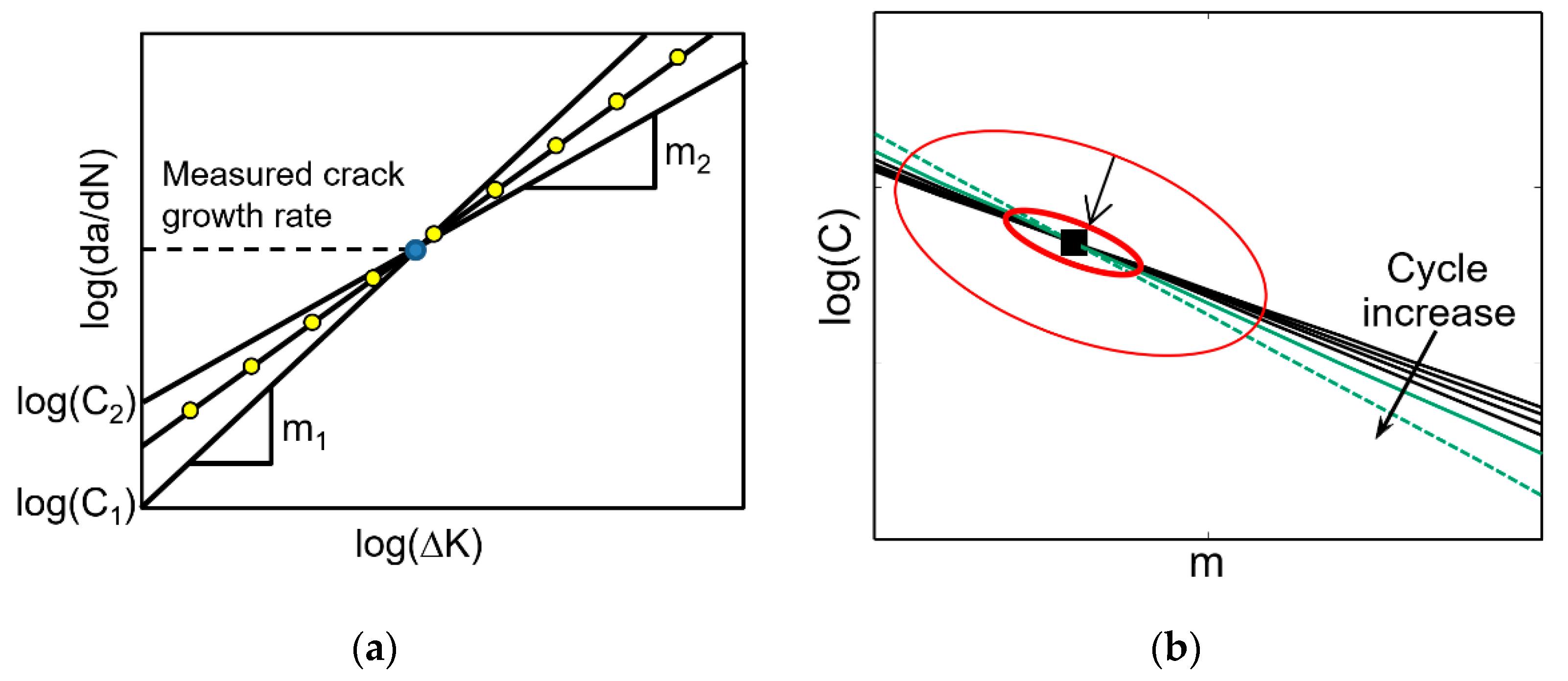
It turned out that the correlation between the two parameters, and , was strong, which means that it would be difficult to identify individual values. Instead, the correlation relationship can be identifiable [16]. Figure 1a shows a log-log scale graph of the crack growth rate versus the range of stress intensity factor. When the crack growth is in a stable stage, the crack growth rate shows a linear trend, which can be determined using the slope and y-intercept .
As shown in Figure 1a, for a given , the measured crack growth rate can be obtained by infinitely many combinations of and . That is, different combinations of and can represent the same crack growth. This is the basic nature of correlation that this paper addresses. Indeed, a functional relation between them can be obtained as:
where and are the true model parameters that we want to identify. The above equation can be considered as a linear relationship between and . Considering Equation (3) as a linear curve, the slope will change as the crack grows.
As the crack grows and the stress intensity factor increases, the correlation line between the two parameters gradually rotates with the true values at the center, which makes the correlation shape to be identified as a narrow-banded ellipse as shown in Figure 1b. If the slopes of two lines are significantly different, the intersection of two lines can be used to identify the true values of model parameters. This characteristic will be used in Section 4 to identify individual model parameters under correlation.
2.2. Correlation between Load Condition and Model Parameters
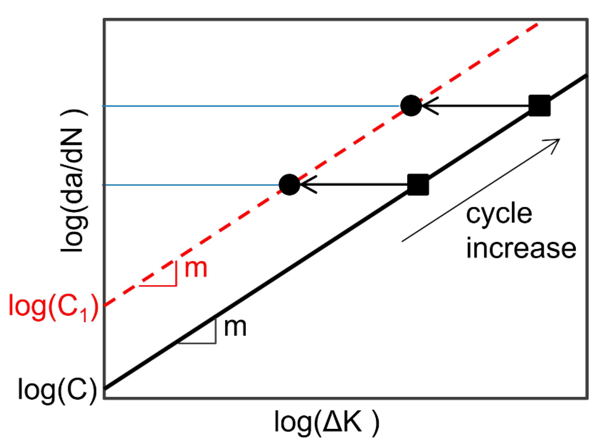
In addition to the correlation between two parameters, another interesting correlation in physics-based models occurs between the applied loadings (operating conditions) and degradation parameters. The black solid line in Figure 2 represents the true crack growth when both applied loadings and degradation parameters are correct. In fatigue crack growth, the range of stress intensity factor, , corresponds to the loading condition. Since depends on the local stress, it is possible that an incorrect stress can be used due to the error in stress calculation. When engineers assume a lower value of , the same observed crack growth can be obtained by increasing the y-intercept from to . That is, the same crack growth can be obtained by decreasing and increasing y-intercept, which is another case of correlation. This linear relationship between and can also be seen from Equation (3) with a fixed .
This kind of correlation is different from that of degradation parameters. The conclusion in the correlation between degradation parameters in the previous section was that even if the true values cannot be identifiable, the correlation allows predicting the RUL properly. Different from the fact that degradation parameters need to be identified, loading conditions are not a part of identification. Rather, they are input conditions. Therefore, this case happens when the information on the applied loading is wrong. If a lower than the actual one is used, the crack growth in the black line moves to the dashed red line in Figure 2. Therefore, a new combination of parameters, and , will be identified as equivalent parameters with a lower stress intensity factor. When the loading remains constant, it is equivalent to correlated parameter identification. Therefore, the equivalent parameters, and , would predict the RUL properly.
In order to show the relationship clearly, let us assume that the exponent is fixed to . Then by taking the logarithm of Equation (1) at two different loading conditions, the following equation can be derived as:
where and are the correct model parameters under .
For practical applications, this correlation and equivalent degradation parameters are in favor of prognostics. It has been mentioned that the model–form error is an important issue in physics-based prognostics. Since most models include assumptions and simplifications, the actual degradation behavior is different from that of the model. Such a model-form error often appears in the form of loading conditions. As an example, it is well-known that the Paris–Erdogan model is designed for an infinite flat plate with a loading direction being perpendicular to the crack. In practice, all plates have a finite size under various boundary conditions. Therefore, the model needs to be modified/corrected to compensate for the effect of geometry, crack shape and location, and boundary conditions. In order to compensate for these effects, the stress intensity factor is modified by:
where is the correction factor, given as the ratio of the true stress intensity factor to the value predicted by . The correction factor depends on the geometry ratio of the crack and plate and the loading conditions. Therefore, the apparent stress intensity factor is different from the correct stress intensity factor . However, the process of identifying model parameters can compensate for this error by identifying equivalent model parameters that can yield the same RUL.
2.3. Correlation between Measurement Bias and Initial Crack Size
When damage is measured using sensors, the signals may have calibration error or the conversion model may have model form error, which leads to bias error. In particular, when a crack is measured using SHM, the exact location of the crack is often unknown. Since the crack size is estimated using the signal strength and since the signal strength depends on the crack location, the estimated crack size may include bias error [24]. In prognostics algorithms, bias can significantly affect predictions. While estimating the crack size, for example, if the estimated crack size is larger than the actual one, this is referred to as a positive bias. Such a positive bias leads to overestimating because the crack size is larger than the true one. When the crack size is large, but the crack growth is the same, the exponent will be underestimated. In the case of a negative bias, it will be overestimated [25].
For simplicity, it is assumed that the bias is a constant, and it needs to be included as an unknown parameter. It is possible that the bias may change as a function of the stress intensity factor, but it would require a more complicated bias function with more unknown parameters. With the physics model for the crack size given in Equation (2) and a constant bias, the relationship between the measured and actual crack sizes can be written as:
where is the unknown bias, and is the actual crack size at loading cycle . When the measurement process has a systematic bias, the stress intensity factor should be calculated using the actual crack size; i.e., .
A new type of correlation occurs between the initial crack size and systematic bias, which will influence the results of the prognostic. In order to show the correlation, let the initial measure crack size be . Under the assumption that the measurement system does not have any noise, the relationship between measured size and the true size can be written as:
Since infinitely many combinations of and can produce the same , linear correlation exists between the two.
3. Model Parameter Estimation Using Bayesian Inference
As previously mentioned, the noise in data makes the identification process difficult. In addition, all three correlations may present simultaneously, which may cause the process more challenging. Although there are many parameter identification methods, such as the least-squares method, the Bayesian method is used in this paper.
In the following explanation, represents the uncertain variable of unknown model parameter, and represents the uncertain variable of the degradation feature. A variable with an upper case denotes an uncertain variable, while a variable with a lower case denotes a realization of the uncertain variable. Bayesian inference estimates the degree of belief in a hypothesis based on collected evidence. Bayes [26] formulated the degree of belief using the following identity in conditional probability:
where is the conditional probability of given . In the case of estimating the model parameter using measured data, the conditional probability of when the probability of measured data is available can be written as:
where is the posterior probability of parameter for given measurement data , and is called the likelihood function or the probability of obtaining data for a given parameter . In Bayesian inference, is called the prior probability, and is the marginal probability of and acts as a normalizing constant. The above equation can be used to improve the knowledge of when additional information is available.
Bayes’ theorem in Equation (9) can be extended to the continuous probability distribution with a probability density function (PDF), which is more appropriate for the purpose of the present paper [27]. Let be a PDF of model parameter . When there are more than one model parameters, can be a joint PDF of multiple parameters. If SHM measures a degradation feature Y, it is also a random variable, whose PDF is denoted by . Then, the joint PDF of and can be written in terms of and , as:
When and are independent, the joint PDF can be written as and Bayesian inference cannot be used to improve the probabilistic distribution of . Using the above identity, the original Bayes’ theorem can be extended to the PDF as [28]:
Since the denominator is a constant and since the integral of is one from the property of PDF, the denominator in Equation (11) can be considered as a normalizing constant. By comparing Equation (11) with Equation (9), is the posterior PDF of parameter given measured data , and is the likelihood function or the PDF value of measured data given model parameter . The process of updating the posterior distribution of model parameter using the measured data is called Bayesian inference.
When multiple, independent data are available, Bayesian inference can be applied for all data at once. When number of measurements are available; i.e., , the Bayes’ theorem in Equation (11) can be modified to:
where is a normalizing constant to make the integral of the posterior PDF equal to one. In the above expression, it is possible that the likelihood functions of individual data are multiplied together to build the total likelihood function, which is then multiplied by the prior PDF followed by normalization to yield the posterior PDF.
An important advantage of Bayes’ theorem over other parameter identification methods, such as the least-squares method and maximum likelihood estimate, is its capability to estimate the uncertainty structure of the identified parameters. These uncertainty structures depend on the prior distribution and likelihood function. Accordingly, the accuracy of the posterior distribution is directly related to that of the likelihood and the prior distribution. Thus, the uncertainty in the posterior distribution must be interpreted in that context.
In the Bayesian method, it is assumed that the users know the prior distribution of model parameters and the distribution type of measurement noise. In this paper, it is assumed that the prior distribution is given as a uniform distribution with a lower- and upper-bound. It is also assumed that the measurement noise has a Gaussian distribution; that is , where s is the standard deviation of the noise. In most cases, since the standard deviation of the noise is unknown, it should be a part of unknown model parameters. In the case of crack growth, the vector of unknown model parameters is defined as . It is also possible that the initial crack size and measurement bias can be included in the unknown model parameters. For the correlation caused by the initial crack size and bias can be found in An et al. [16]. The prior distribution of each parameter is assumed as a uniform distribution. By assuming that all model parameters are statistically independent, the prior joint PDF of the parameters can be defined as:
The posterior distribution can be obtained by multiplying the prior distribution with the likelihood function.
With the given prior distribution, the next step is to calculate the likelihood function using the measured data, as shown in Equation (12). The definition of the likelihood function is the probability (in this case the value of PDF) of obtaining the measured data for given model parameters . Since the measured data are fixed, the likelihood function is a function of model parameters. If the model prediction is close to the measured data, then the likelihood is large, while the likelihood is small when the two values are significantly different. To build the likelihood, it is necessary to compare the measured degradation with the predicted one from the model. Since the measured degradation data are given at discrete times, the degradation model is also evaluated at the same discrete times as . It is noted that since the degradation model is evaluated at discrete times tk, is only a function of model parameters and . The measured data include the random noise that is governed by , while the model prediction depends on and . Then, the likelihood function of the k-th measured data can be defined as:
When multiple measured data are present, the likelihood of individual data are multiplied together as shown in Equation (12). With Ndata data, , the posterior joint PDF can be calculated by multiplying all likelihood functions with the prior PDF as:
where is a normalizing constant.
The posterior distribution in Equation (15) can be estimated using a sampling method, such as the Markov-chain Monte-Carlo simulation. However, since the goal is to identify accurate model parameters, a grid method is used to show the posterior PDF. In order to present the results in 2D graph, the third parameter, s, is integrated over its range. The posterior joint PDF is calculated at a 100 × 100 grid. The marginal distribution is calculated by integrating each variable using the grid values.
4. Identification of Correlated Model Parameters
In this section, the fatigue crack growth data presented in Forman et al. [29] are used to estimate the damage growth model parameters. Section 4.1 presents the first method of identifying model parameters using two different stages of crack growth, while Section 4.2 presents the second method of identifying model parameters using two different operating conditions.
4.1. Identification of Correlated Model Parameters Using Two Different Stages
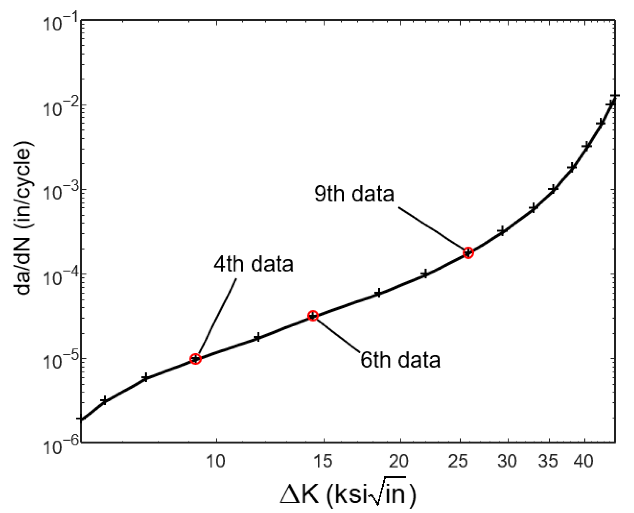
Figure 3 shows the measured fatigue crack growth rate of AL 7075-T651 plate, where the 4th and 9th data are used to show the process of model parameter identification. Without knowing the true model parameters, Equation (3) cannot be used for the identification process. Instead, the logarithmic version of Equation (1) is used, as:
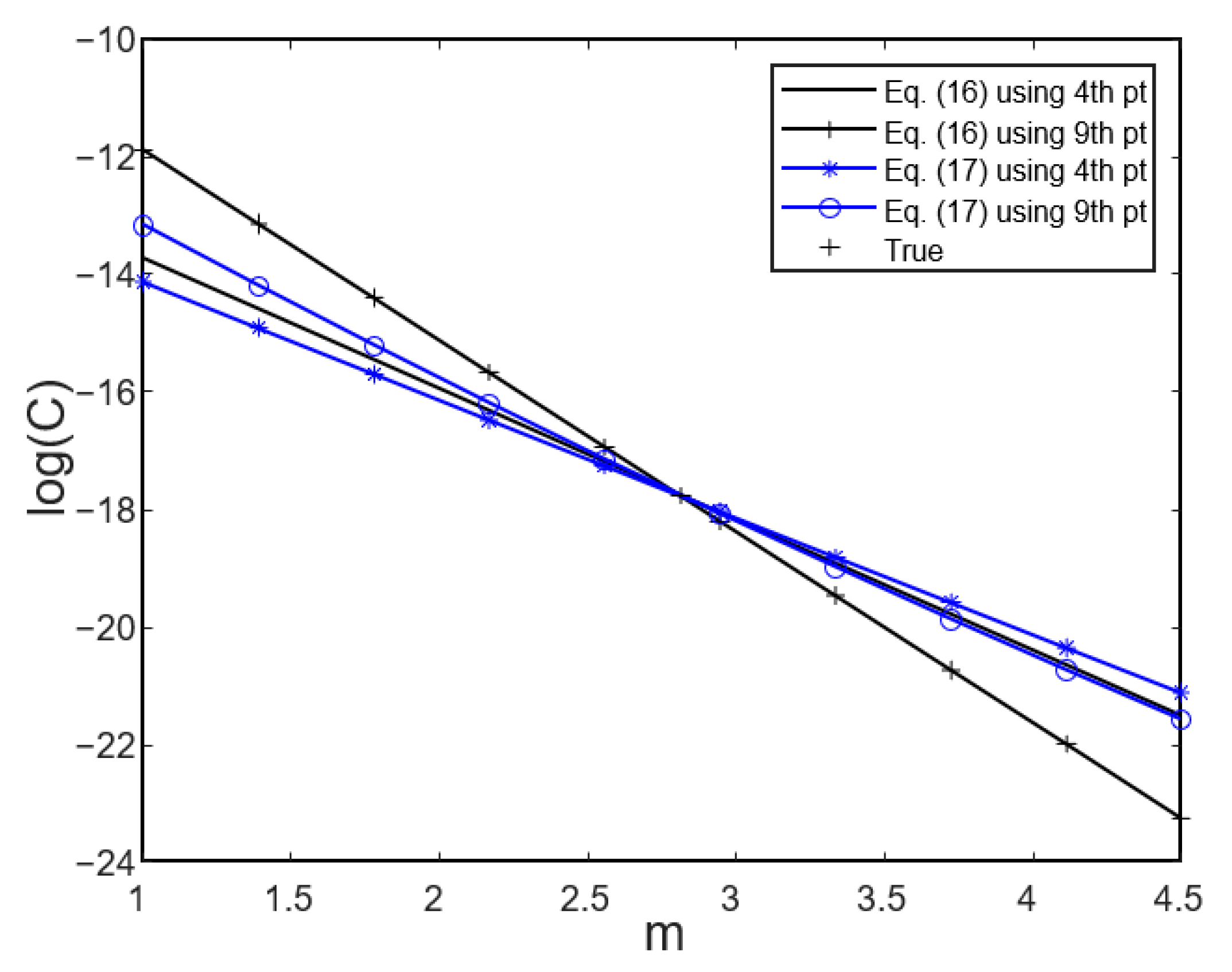
With given and data, Equation (16) yields an equation of line between and . That is, with a measured crack growth rate, it is impossible to identify the two model parameters because they are perfectly correlated. However, if two different crack growth rates are measured, then they can perfectly determine the two model parameters. For example, two black-colored lines in Figure 4 show the linear relationships in Equation (16) at the fourth and ninth data points. These two lines intersect at and (cross marker), which is considered as the true model parameters in this paper.
The above process of identifying multiple model parameters has two idealized assumptions that cannot easily be overcome in structural health monitoring. Firstly, the current state-of-the-art SHM sensors can measure the crack size, not the crack growth rate. Secondly, the measured crack size includes a significant amount of noise. Small noise and error in data can significantly affect the identification results. For the first difficulty, the linear relationship in Equation (16) has to be revised in terms of measured crack size. By taking the logarithm of Equation (2), the relationship between and can be obtained when a crack size of is measured, as:
Although the relationship is nonlinear, and the expression seems complicated, it actually shows almost a linear relationship as shown in Figure 4. In addition, the intersection between the two blue-colored curves is identical to the identified true parameters. Therefore, the measured crack sizes at different sizes can be used to identify the correlated model parameters.
The second challenge is related to the noise in measured data. The data provided in Figure 3 are measured manually in the laboratory. When sensors in an SHM system are used to measure the crack size, there is inevitably noise in the measurement. In addition, the effect of noise in measured crack size is amplified further in crack growth rate, . Although there are many different ways of identifying model parameters under noisy measurements, Bayesian inference in Section 3 is utilized here. First, from the true values of model parameters, and , simulated measurement data are generated around fourth and ninth points in Figure 3, where and . In the interval of , 20 simulated measurement data are generated, while in the interval of , five simulated measurement data are generated. More data are generated around because the crack grows slowly in the early stage, and more data are required in the inference process. All data are generated using the true model parameters and added random noise . The magnitude of the standard deviation of the noise, 0.15 in, is significant compared to the initial crack size of 0.097 in. The true model parameters are only used for the purpose of generating data, not in the inference process.
For the prior, a uniform distribution is assumed for and , independence assumption as in Equation (13) is used. These prior distributions were obtained using the lower- and upper-bounds of all test data in Forman et al. [29] for AL 7075-T651 under various load ratios. This uniform distribution and independence assumption are used because they are considered as a prior knowledge.
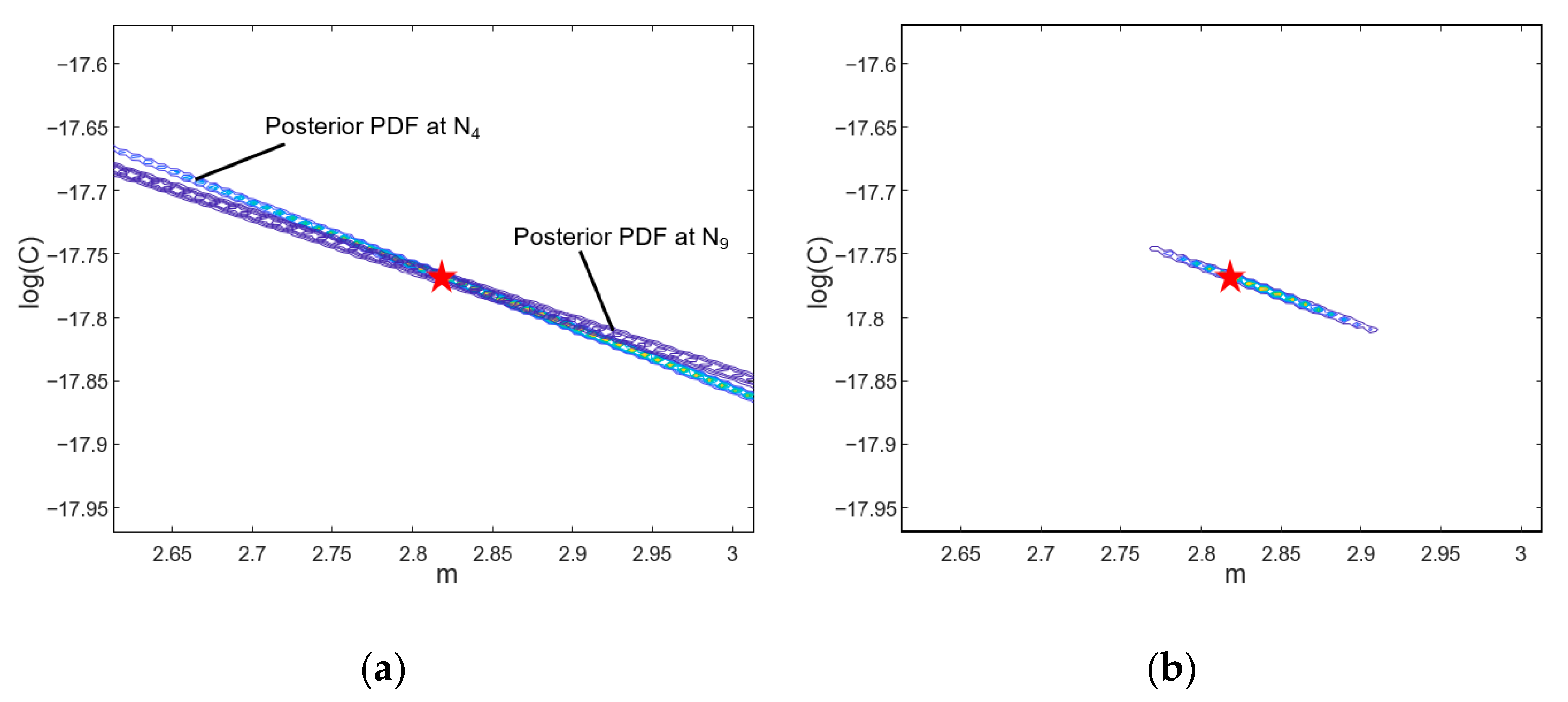
Using the likelihood function that is calculated using the measured data, the posterior distribution can be obtained using Equation (15). Figure 5a shows the posterior joint distributions that are obtained separately using 20 data around and 5 data around . As explained before, due to the strong correlation, the posterior distribution shows a narrow-banded shape, where it is difficult to identify the model parameters. If the marginal distribution is calculated, the distribution is almost identical to the prior distribution. This happens because of the strong correlation between the two parameters. In addition, the peaks of individual posterior distributions do not match with the true parameter values in the start marker. As shown in Figure 5b, however, the combined posterior distributions with and converges to the true values of model parameters, which is shown with a star marker. If the marginal distributions are calculated, and . Therefore, the uncertainties for both parameters are significantly reduced compared to the posterior distributions from individual case in Figure 5a, and the mean values are close to the true model parameters. Table 1 compares the uncertainty reduction by combining the two posterior distributions in the form of the standard deviation of the marginal distribution. The uncertainty in parameter is reduced by four times, while that in is three times.
When two different crack sizes are used, the performance of uncertainty reduction is significant as the difference between the two crack sizes is large. This is because the slope depends on the crack size . However, there is a limitation of crack size because as the crack size increases, the crack grows quickly, and the plate is near the fracture. Therefore, it is important to consider two significantly different crack sizes but not too close to the fracture.
4.2. Identification of Correlated Model Parameters Using Two Different Loading Conditions
The second method of identifying the accurate values of model parameters under correlation is related to changing the loading conditions. In order to show the correlation between the model parameters and loading conditions in Section 2.2, the same Paris model in the previous section is used with the data shown in Figure 3. Since it is unnecessary to use data at two different crack growth rates, a single 6th data point is used, where the consumed cycles are , the crack size , the range of stress intensity factor , and the crack growth rate .
Since the stress intensity factor is the function of stress and crack size, it is possible to change the level of stress while keeping the same stress intensity factor. Therefore, it is assumed that the first case is when , while the second case is when . In the industry, this kind of two amplitude loadings is common. For example, in a gas turbine power plant, the system is operated in nominal conditions most of the time, but during the peak season, the system is operated in the maximum loading conditions. Such a change in operating conditions can be used to identify the correlated model parameters.
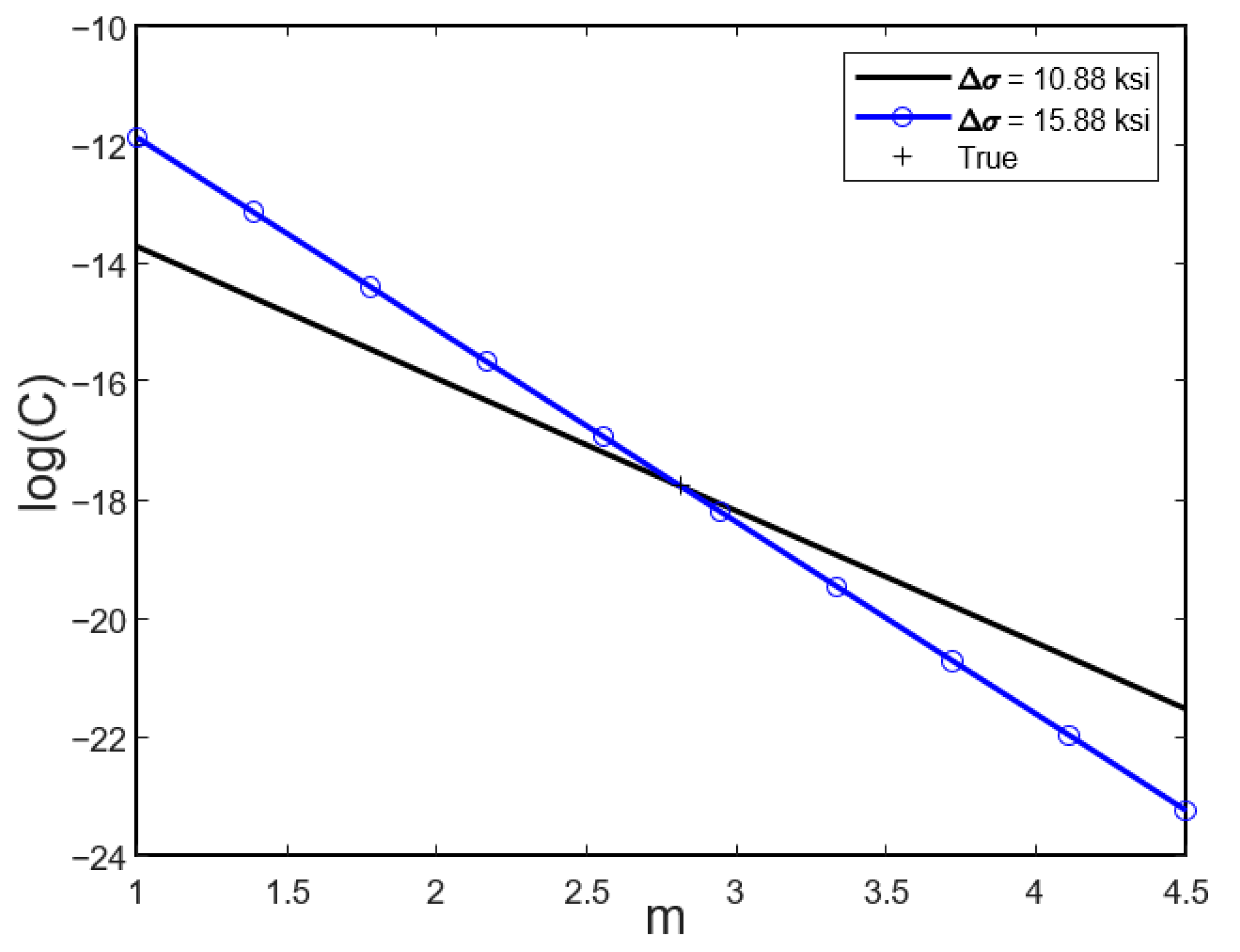
The correlation relationship in Equation (4) cannot be used here because it requires the knowledge of the true model parameters. Instead, Equation (16) is used to show the nature of correlation and how to identify the accurate model parameters. It is noted that Equation (17) can also be used, but it will produce identical results. The linear relationship between and in Equation (16) is plotted at two different loading conditions, and , in Figure 6. As expected, the two correlation lines meet at the true model parameters. Therefore, measuring crack growth rates at different loading conditions can be used to identify the correlated model parameters.
The identification of model parameters as in Figure 6 has two challenges in practice. The first challenge is the fact that the crack growth rates at different loading conditions cannot be measured simultaneously. Therefore, a possible way is to measure the crack growth before and after the loading condition changes. For that purpose, starting from the 6th data (N6 = 40,886 cycles) in Figure 3, 20 crack size data are generated during 12,000 cycles under the nominal operating condition . Then, it is assumed that the loading condition is increased to the maximum operating condition , and 5 crack size data are generated during the next 4000 cycles. Like the previous example, synthetic data are generated based on the true model parameters. Random noise is added to all data.
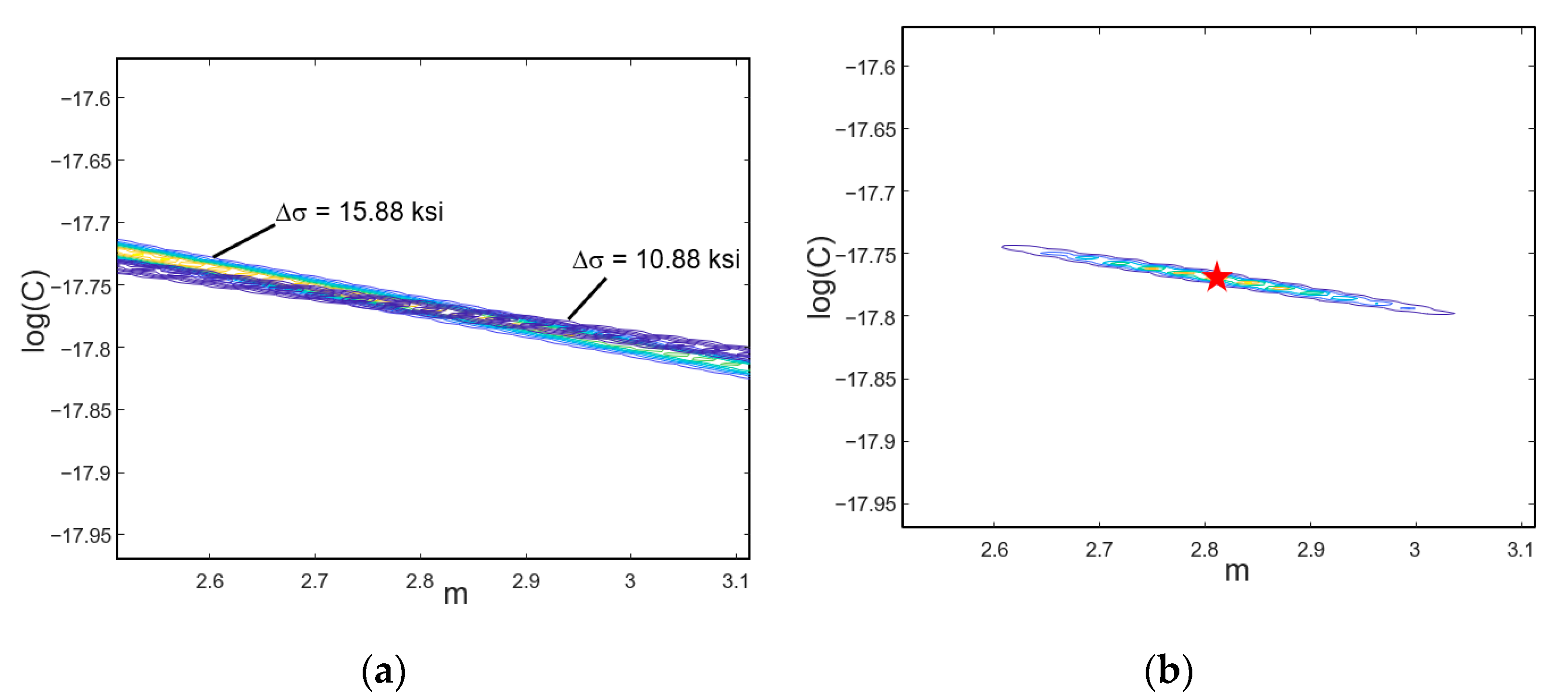
Figure 7a shows the two posterior joint distributions that are obtained separately using two sets of data. Even if two datasets are located closely, the correlation line in Figure 7a shows a significant difference. This is due to the fact that the crack growth rates are significantly different. When the two posterior PDFs are multiplied, Figure 7b shows a much better identification of the two model parameters. The marginal distributions are estimated as and . Therefore, the uncertainties for both parameters are significantly reduced, and the mean values are close to the true model parameters. Table 2 compares the uncertainty reduction by combining the two posterior distributions in the form of the standard deviation of the marginal distribution. The uncertainty in parameter is reduced by ten times, while that in is three times.
In theory, two lines with different slopes can have a single intersection, which corresponds to the identified model parameters. In practice, however, the noise in data makes the line a probability distribution, and the width of the distribution increases proportionally to the level of noise. Therefore, it would require more data to clearly identify individual parameters. In addition, if the difference in slopes is small, the intersection region will be large, as shown in Figure 7b. This happens in the early stage of crack growth where the cracks grow slowly. A better identification can be achieved in the region where the crack grows fast. The performance of uncertainty reduction is improved proportionally to the difference between load amplitudes. This is also because the slope depends on the load amplitude .
5. Conclusions
In this paper, we showed that it is challenging to identify model parameters of physics-based prognostics when they are strongly correlated. We illustrated this aspect using the fatigue crack growth example, where common correlations occur between model parameters, between model parameter and loading conditions, and between initial damage size and measurement bias. By utilizing the fact that the correlation structure evolves at different damage sizes or different loading conditions, the paper proposes two methods of identifying model parameters accurately even if they show a strong correlation. By utilizing different damage sizes, the standard deviation of the marginal distribution of exponent is reduced from 0.125 to 0.03. When different loading conditions are used, it is reduced from 0.3 to 0.05. Since both results were obtained under a significant level of noise, the standard deviation of 0.15 in, the proposed methods were effective in reducing the uncertainty of correlated parameters. The performance of uncertainty reduction will be more significant if the difference in the two crack sizes and the two loads is large.
Author Contributions
Conceptualization, N.H.K.; methodology, T.D.; software, T.D.; validation, N.H.K.; formal analysis, T.D.; investigation, T.D.; resources, N.H.K.; data curation, T.D.; writing—original draft preparation, T.D.; writing—review and editing, N.H.K.; visualization, T.D.; supervision, N.H.K. All authors have read and agreed to the published version of the manuscript.
Funding
This research received no external funding.
Institutional Review Board Statement
Not applicable.
Informed Consent Statement
Not applicable.
Data Availability Statement
All data in this paper were numerically generated using random number generator.
Conflicts of Interest
The authors declare no conflict of interest.
References
- Kessler, S.S. Certifying a structural health monitoring system: Characterizing durability, reliability and longevity. In Proceedings of the 1st International Forum on Integrated Systems Health Engineering and Management in Aerospace, Napa, CA, USA, 7–10 November 2005; pp. 7–10. [Google Scholar]
- Jardine, A.K.; Lin, D.; Banjevic, D. A review on machinery diagnostics and prognostics implementing condition-based maintenance. Mech. Syst. Signal Process. 2006, 20, 1483–1510. [Google Scholar] [CrossRef]
- Giurgiutiu, V. Structural Health Monitoring with Piezoelectric Wafer Active Sensors; Academic Press: Cambridge, MA, USA, 2008. [Google Scholar]
- Sohn, H.; Farrar, C.R.; Hemez, F.M.; Czarnecki, J.J.; Shunk, D.D.; Stinemates, D.W.; Nadler, B.R. A Review of Structural Health Monitoring Literature: 1996–2001; Report Number LA-13976-MS; Los Alamos National Laboratory: Los Alamos, NM, USA, 2004. [Google Scholar]
- Dong, T.; Kim, N.H. Cost-effectiveness of structural health monitoring in fuselage maintenance of civil aviation industry. Aerospace 2018, 5, 87. [Google Scholar] [CrossRef] [Green Version]
- Bukenya, P.; Moyo, P.; Beushausen, H.; Oosthuizen, C. Health monitoring of concrete dams: A literature review. J. Civ. Struct. Health Monit. 2014, 4, 235–244. [Google Scholar] [CrossRef]
- Pentaris, F.P.; Stonham, J.; Makris, J.P. A review of the state-of-the-art of wireless SHM systems and an experimental set-up towards an improved design. Eurocon 2013, 2013, 275–282. [Google Scholar] [CrossRef]
- Staszewski, W.J.; Boller, C.; Tomlinson, G.R. Health Monitoring of Aerospace Structures: Smart Sensor Technologies and Signal Processing; Wiley & Sons: Hoboken, NJ, USA, 2004. [Google Scholar]
- Farrar, C.R.; Lieven, N.A.J. Damage prognosis: The future of structural health monitoring. Philos. Trans. R. Soc. A 2006, 365, 623–632. [Google Scholar] [CrossRef] [PubMed]
- Kim, N.H.; An, D.; Choi, J. Prognostics and Health Management of Engineering Systems: An Introduction; Springer International Publishing: Cham, Switzerland, 2017. [Google Scholar] [CrossRef]
- An, D.; Kim, N.H.; Choi, J.-H. Practical options for selecting data-driven or physics-based prognostics algorithms with reviews. Reliab. Eng. Syst. Saf. 2015, 133, 223–236. [Google Scholar] [CrossRef]
- Wang, P.; Youn, B.D.; Hu, C. A generic probabilistic framework for structural health prognostics and uncertainty management. Mech. Syst. Signal Process. 2012, 28, 622–637. [Google Scholar] [CrossRef]
- Baraldi, P.; Compare, M.; Sauco, S.; Zio, E. Ensemble neural network-based particle filtering for prognostics. Mech. Syst. Signal Process. 2013, 41, 288–300. [Google Scholar] [CrossRef] [Green Version]
- Lim, C.K.R.; Mba, D. Switching Kalman filter for failure prognostic. Mech. Syst. Signal Process. 2015, 52–53, 426–435. [Google Scholar] [CrossRef]
- Gašperin, M.; Juričić, Đ.; Boškoski, P.; Vižintin, J. Model-based prognostics of gear health using stochastic dynamical models. Mech. Syst. Signal Process. 2011, 25, 537–548. [Google Scholar] [CrossRef]
- An, D.; Choi, J.; Kim, N.H. Identification of correlated damage parameters under noise and bias using Bayesian inference. Struct. Health Monit. 2012, 11, 293–303. [Google Scholar] [CrossRef]
- An, D.; Choi, J.; Kim, N.H. Prognostics 101: A tutorial for particle filter-based prognostics algorithm using Matlab. Reliab. Eng. Syst. Saf. 2013, 115, 161–169. [Google Scholar] [CrossRef]
- Gelman, A.; Carlin, J.B.; Stern, H.S.; Dunson, D.; Vehtari, A.; Rubin, D. Bayesian Data Analysis; Chapman & Hall: New York, NY, USA, 2004. [Google Scholar]
- Li, P.; Vu, Q.D. Identification of parameter correlations for parameter estimation in dynamic biological models. BMC Syst. Biol. 2013, 7, 91. [Google Scholar] [CrossRef] [PubMed] [Green Version]
- Santos, T.J.; Pinto, J.C. Taking variable correlation into consideration during parameter estimation. Braz. J. Chem. Eng. 1998, 15. [Google Scholar] [CrossRef]
- Matzke, D.; Ly, A.; Selker, R.; Weeda, W.D.; Scheibehenne, B.; Lee, M.D.; Wagenmakers, E. Bayesian inference for correlations in the presence of measurement error and estimation uncertainty. Collabra Psychol. 2017, 3, 25. [Google Scholar] [CrossRef]
- Swanson, D.C.; Spencer, J.M.; Arzoumanian, S.H. Prognostic modelling of crack growth in a tensioned steel band. Mech. Syst. Signal Process. 2000, 14, 789–803. [Google Scholar] [CrossRef]
- Park, C.; Kim, N.H.; Haftka, R.T. The effect of ignoring dependence between failure modes on evaluating system reliability. Struct. Multidiscip. Optim. 2015, 52, 251–268. [Google Scholar] [CrossRef]
- An, J.; Haftka, R.T.; Kim, N.H.; Yuan, F.G.; Kwak, B.M.; Sohn, H.; Yeum, C.M. Experimental study on identifying cracks of increasing size using ultrasonic excitation. Struct. Health Monit. 2012, 11, 95–108. [Google Scholar] [CrossRef]
- Coppe, A.; Haftka, R.T.; Kim, N.H.; Yuan, F. Uncertainty reduction of damage growth properties using structural health monitoring. J. Aircr. 2010, 47, 2030–2038. [Google Scholar] [CrossRef]
- Bayes, T.; Price, R. An Essay towards solving a problem in the doctrine of chances. By the late Rev. Mr. Bayes, communicated by Mr. Price, in a let-ter to John Canton, A.M.F.R.S. Philos. Trans. R. Soc. Lond. 1763, 53, 370–418. [Google Scholar] [CrossRef]
- An, D.; Choi, J.; Kim, N.H.; Pattabhiraman, S. Fatigue life prediction based on Bayesian approach to incorporate field data into probability model. Struct. Eng. Mech. 2011, 37, 427–442. [Google Scholar] [CrossRef] [Green Version]
- Athanasios, P. Probability, Random Variables, and Stochastic Processes; McGraw-Hill: New York, NY, USA, 1984. [Google Scholar]
- Forman, R.G.; Shivakumar, V.; Cardinal, J.W.; Williams, L.C.; McKeighan, P.C. Fatigue Crack Growth Database for Damage Tolerance Analysis; Final report DOT/FAA/AR-05/15; Federal Aviation Administration: Washington, DC, USA, 2005. [Google Scholar]
Figure 1.
Correlation in model parameters and its evolution; (a) same crack growth rate with different combinations of parameters; (b) evolving correlation relationship with respect to cycles.
Figure 1.
Correlation in model parameters and its evolution; (a) same crack growth rate with different combinations of parameters; (b) evolving correlation relationship with respect to cycles.

Figure 2.
Overestimation of log(C) due to underestimation of stress intensity factor.

Figure 3.
Fatigue crack growth rate for AL 7075-T651 plate [29].
Figure 3.
Fatigue crack growth rate for AL 7075-T651 plate [29].

Figure 4.
Two correlation lines at different crack growth rates with the true model parameters.

Figure 5.
Posterior joint distributions of and . (a) around and cycles, and (b) combined posterior distribution.
Figure 5.
Posterior joint distributions of and . (a) around and cycles, and (b) combined posterior distribution.

Figure 6.
Two correlation lines at different loading conditions with the true model parameters.

Figure 7.
Posterior joint distributions of and . (a) Nominal and maximum operating conditions, and (b) combined posterior distribution.
Figure 7.
Posterior joint distributions of and . (a) Nominal and maximum operating conditions, and (b) combined posterior distribution.


Table 1.
Comparison of standard deviation (STD) of model parameters using two different stages.
| Conditions | STD of | STD of |
|---|---|---|
| Using 20 data around N4 | 0.125 | 0.06 |
| Using 5 data around N9 | 0.14 | 0.06 |
| Combined posterior dist. | 0.03 | 0.02 |
Table 2.
Comparison of standard deviation (STD) of model parameters using two different loading conditions.
Table 2.
Comparison of standard deviation (STD) of model parameters using two different loading conditions.
| Conditions | STD of | STD of |
|---|---|---|
| 0.3 | 0.06 | |
| 0.3 | 0.06 | |
| Combined posterior dist. | 0.05 | 0.02 |
Publisher’s Note: MDPI stays neutral with regard to jurisdictional claims in published maps and institutional affiliations. |
© 2021 by the authors. Licensee MDPI, Basel, Switzerland. This article is an open access article distributed under the terms and conditions of the Creative Commons Attribution (CC BY) license (https://creativecommons.org/licenses/by/4.0/).
Share and Cite
MDPI and ACS Style
Dong, T.; Kim, N.H. Methods of Identifying Correlated Model Parameters with Noise in Prognostics. Aerospace 2021, 8, 129. https://0-doi-org.brum.beds.ac.uk/10.3390/aerospace8050129
AMA Style
Dong T, Kim NH. Methods of Identifying Correlated Model Parameters with Noise in Prognostics. Aerospace. 2021; 8(5):129. https://0-doi-org.brum.beds.ac.uk/10.3390/aerospace8050129
Chicago/Turabian StyleDong, Ting, and Nam H. Kim. 2021. "Methods of Identifying Correlated Model Parameters with Noise in Prognostics" Aerospace 8, no. 5: 129. https://0-doi-org.brum.beds.ac.uk/10.3390/aerospace8050129
Note that from the first issue of 2016, this journal uses article numbers instead of page numbers. See further details here.