Three-Surface Model with Redundant Longitudinal Control: Modeling, Trim Optimization and Control in a Preliminary Design Perspective

Abstract

Notwithstanding the interest in the three-surface concept shown by aircraft designers, this configuration was not thoroughly investigated in conjunction with the adoption of two-elevator surfaces, on both canard and tail. In fact, the inclusion of an additional elevator produces a redundant longitudinal control which can be specifically exploited to target trim optimization. The same redundancy can be also employed to improve the flying qualities of the three-surface aircraft. In this paper, after introducing a simple flight mechanics model, ideal for preliminary design and analyses, the advantages of this configuration are explored. Firstly, the problem of finding the elevator deflections of canard and tail for minimum drag in trim is formulated and solved. Secondarily, the updating of a two-surface back-tailed airplane into an equivalent three-surface one is demonstrated, showing the potential improvement in cruise performance. Finally, the controls are employed through a smart control law for achieving better flying qualities.

1. Introduction

Examples of aircraft featuring a three-surface configuration have indeed existed since the early stages of aviation, a noteworthy successful example from the era being the Curtiss N.2 which flew in 1909. Since then, this configuration has surfaced several times along the evolution of aviation design. With the exception of warplanes, where this configuration has been adopted in the quest for better maneuverability (like in the experimental McDonnell-Douglas F-15 STOL/MTD or the production Sukhoi Su-30, Su-33 and Su-34), it has however been met with limited popularity, especially in civil aviation, where the only large scale production example is the Piaggio P-180 Avanti from the 1980s. The reason for the reduced spreading of this configuration may be searched in the general mistrust of aircraft manufacturers in a departure from traditional and successful designs, as well as the risk of a lower public acceptance for a less common configuration [1]. In fact, the adoption of a three-surface configuration on civil aircraft enables the achievement of some unquestionable technical advantages. The most obvious and worth citing are a generally lower wing and tail area, thanks to the addition of a surface ahead of the center of mass producing positive lift, which if properly sized, should produce reduced induced drag, and a mitigation of the erosion of the static margin typical to purely canard configurations, which bear the greatest advantages in terms of drag minimization in cruise.

Despite the comparatively generally lower interest raised by this configuration shown by manufacturers of civil aircraft, there exists a good knowledge base, investigating this type of design since a few decades ago. In the works of Agnew and Kendall [2,3,4] the aerodynamics of three-surface aircraft and their impact on flight mechanics performance are investigated on very simplified testbeds with no control on the canard surface. In [4], it is shown a significant potential drag advantage for the case of a configuration very similar to the Piaggio P-180, in particular without a continuous deflection of the trailing edge surfaces of the canard (the real aircraft actually implements a discrete control of the canard elevator, conceptually similar to a wing flap).

Early experimental testing, comparing different configurations and assessing the respective potential advantages, are reported in [5].

The idea has been retrieved also more recently at a conceptual level [6], as well as in more advanced studies, concerned with aero-elastic stability and structural control [7,8], the latter achieved also by means of a dedicated use of fully pivoting canard surfaces.

In the current quest for more fuel-efficient designs, one of the advantages of a three-surface configuration is of great potential interest, i.e., the chance to optimize cruise performance. This would yield the result of lower emissions as well as fuel expenditure, making this type of aircraft an advantageous and realistic solution towards commercially viable and energetically efficient aviation [9,10].

To this aim, the introduction of an elevator control surface located at the trailing edge of the canard, used in conjunction with the control surfaces typically mounted on more widespread back-tailed aircraft, generates a redundant longitudinal control to be exploited for pursuing an optimal performance. Moreover, the same type of control configurations can be used to condition the dynamics of the aircraft in such a way to re-obtain a dynamic performance very closely resembling that of a traditional aircraft. This would mitigate the need for specific pilot type rating, and increase safety by avoiding the introduction of different dynamics with respect to existing aircraft and easing pilot’s operations.

To explore and demonstrate these possibilities, the present paper introduces a complete flight mechanics model for the longitudinal behavior of a three-surfaces aircraft, featuring trailing-edge elevators on both the canard and horizontal tail. The model is then exploited to demonstrate, in a rigorous mathematical way, the existence and the qualities of an optimal cruise condition. It will be shown how the redundancy in longitudinal control plays a prominent role in the achievement of the desired performance. A parametric update of a baseline aircraft, a Diamond DA42 Twin Star twin engine aircraft [11], to a three-surface configuration is then proposed. The update process is carried out with stringent hypotheses yielding an equivalence of the resulting machine with respect to the traditionally shaped, existent baseline, so as to show the actual advantage brought in by the inclusion of a canard. In a final stage, the dynamic model of the aircraft is further exploited to design a controller suitable for the task of reassigning the dynamics of the three-surface aircraft, to the aim of reproducing that of the back-tailed, two-surface baseline.

2. Flight Mechanics Models for a Three-Surface Aircraft

As explained in the introduction, the present research deals with both static and dynamic performance of a three-surface aircraft. In order to develop the optimal analysis of trim in cruise, a characterization of the aircraft via a static model, based on lumped lift and aerodynamic moment components, is a required asset. This will be introduced in Section 2.1. For dynamic analyses, a classical rigid model for longitudinal aircraft dynamics will be employed, modified to account for the presence of the canard elevator deflection. This will be introduced in Section 2.2, making use of some notions previously included in Section 2.1.

2.1. Static Lumped Model for a Three-Surface Aircraft

Figure 1 displays the adopted geometrical scheme for the lumped model needed for static flight mechanics analyses of a three-surface aircraft. Distances $l_c^{\prime }$ and $l_t^{\prime }$ are defined respectively between the aerodynamic centers of the canard surface ${\mathit{AC}}^c$ and the center of gravity $\mathit{CG}$, and between the latter and the aerodynamic center of the tail ${\mathit{AC}}^t$. The distance between $\mathit{CG}$ and the aerodynamic center of the wing ${\mathit{AC}}^w$ is defined as $l_w^{\prime }$. Distances $l_c$ and $l_t$ are defined between ${\mathit{AC}}^c$ and ${\mathit{AC}}^w$, and between the latter and ${\mathit{AC}}^t$ respectively.

In Figure 1, the distribution of aerodynamic forces on each of the three surfaces is represented by an equivalent lift force, $L^c$, $L^w$ and $L^t$, as well as a pitching moment measured about the aerodynamic center of the corresponding lifting surface, namely ${\mathcal{M}}_{{\mathit{AC}}^c}^c$, ${\mathcal{M}}_{{\mathit{AC}}^w}^w$ and ${\mathcal{M}}_{{\mathit{AC}}^t}^t$, respectively for the canard, wing and tail.

Correspondingly, each surface generates also a drag force, noted as $D^c$, $D^w$ and $D^t$ for the canard, wing and tail respectively (not displayed for simplicity).

Total lift, drag and moment, the latter measured about a generic point $\mathit{P}$, for the three-surface aircraft can be written as

$$\left\{\begin{array}{c}L=L^w+L^t+L^c\hfill \\ D=D^w+D^t+D^c\hfill \\ {\mathcal{M}}_{\mathit{P}}={\mathcal{M}}_{\mathit{P}}^w+{\mathcal{M}}_{\mathit{P}}^t+{\mathcal{M}}_{\mathit{P}}^c\hfill \end{array}\right.,$$

(1)

wherein the terms pertaining to each of the surfaces can be developed as typical for aerodynamic forces and moments, based on a dynamic pressure term $q_d$, a reference surface S, and a non-dimensional force/moment coefficient. For moments, also a length is needed in the dimensional term, and this is the chord $\overline{c}$ of the corresponding surface. This yields

$$\begin{array}{ccccc}\left\{\begin{array}{c}{L}^w=q_{d}S{C}_L^w\hfill \\ L^t=q_d^t{S}^t{C}_L^t\hfill \\ L^c=q_d^c{S}^c{C}_L^c\hfill \end{array}\right.,& & \left\{\begin{array}{c}{D}^w=q_{d}S{C}_D^w\hfill \\ D^t=q_d^t{S}^t{C}_D^t\hfill \\ D^c=q_d^c{S}^c{C}_D^c\hfill \end{array}\right.,& & \left\{\begin{array}{c}{\mathcal{M}}_{\mathit{P}}^w=q_{d}S\overline{c}{C}_{{\mathcal{M}}_{\mathit{P}}}^w\hfill \\ {\mathcal{M}}_{\mathit{P}}^t=q_d^t{S}^t{\overline{c}}^t{C}_{{\mathcal{M}}_{\mathit{P}}}^t\hfill \\ {\mathcal{M}}_{\mathit{P}}^c=q_d^c{S}^c{\overline{c}}^c{C}_{{\mathcal{M}}_{\mathit{P}}}^c\hfill \end{array}\right..\end{array}$$

(2)

In Equation (2), $q_d$ and S pertain to the wing, whereas $q_d^t$ and $S^t$ to the tail, and $q_d^c$ and $S^c$ to the canard.

By extracting the dimensional term $q_{d}S\overline{c}$ in the expressions of forces and moments (Equation (2)), and by substituting in the total lift, drag and moments in Equation (1), the following is obtained

$$\left\{\begin{array}{c}L=q_{d}S\left(C_L^w+{\eta }^t{\sigma }^t{C}_L^t+{\eta }^c{\sigma }^c{C}_L^c\right)\hfill \\ D=q_{d}S\left(C_D^w+{\eta }^t{\sigma }^t{C}_D^t+{\eta }^c{\sigma }^c{C}_D^c\right)\hfill \\ {\mathcal{M}}_{\mathit{P}}=q_{d}S\left(C_{{\mathcal{M}}_{\mathit{P}}}^w+{\eta }^t{\sigma }^t{\kappa }^t{C}_{{\mathcal{M}}_{\mathit{P}}}^t+{\eta }^c{\sigma }^c{\kappa }^c{C}_{{\mathcal{M}}_{\mathit{P}}}^c\right)\hfill \end{array}\right.,$$

(3)

wherein parameters ${\eta }^t$, ${\eta }^c$, ${\sigma }^t$, ${\sigma }^c$, ${\kappa }^t$, ${\kappa }^c$ are defined as follows

$${\eta }^t:=\frac{q_d^t}{q_d},{\sigma }^t:=\frac{S^t}{S},{\kappa }^t:=\frac{{\overline{c}}^t}{\overline{c}},{\eta }^c:=\frac{q_d^c}{q_d},{\sigma }^c:=\frac{S^c}{S},{\kappa }^c:=\frac{{\overline{c}}^c}{\overline{c}}.$$

(4)

Finally, the non-dimensional total lift and moment coefficients can be defined from Equation (3) as

$$\left\{\begin{array}{c}{C}_L=C_L^w+{\eta }^t{\sigma }^t{C}_L^t+{\eta }^c{\sigma }^c{C}_L^c\hfill \\ C_D=C_D^w+{\eta }^t{\sigma }^t{C}_D^t+{\eta }^c{\sigma }^c{C}_D^c\hfill \\ C_{{\mathcal{M}}_{\mathit{P}}}=C_{{\mathcal{M}}_{\mathit{P}}}^w+{\eta }^t{\sigma }^t{\kappa }^t{C}_{{\mathcal{M}}_{\mathit{P}}}^t+{\eta }^c{\sigma }^c{\kappa }^c{C}_{{\mathcal{M}}_{\mathit{P}}}^c\hfill \end{array}\right..$$

(5)

The controls adopted in the current model are the deflection of the canard and that of the horizontal tail, respectively, ${\delta }_c$ and ${\delta }_e$. Both are positive downward, and can be actuated with continuity over a range of positive and negative values, just like the tail elevator control on usual aircraft.

The dependencies of the coefficients in Equation (5) with respect to the angle of attack $\alpha$ of the aircraft and the two elevator controls will be investigated next, separately for lift, drag and pitching moment.

2.1.1. Lift for a Three-Surface Aircraft

Based on the considered scheme (see Equation (5)), as usual a linear dependency of lift coefficients of the three lifting surfaces on the respective angles of attack (${\alpha }^c$, ${\alpha }^w$ and ${\alpha }^t$ for the canard, wing and tail respectively), as well as on ${\delta }_c$ and ${\delta }_e$, is assumed as per Equation (6)

$$\left\{\begin{array}{c}{C}_L^w=C_{L_{{\alpha }^w}}^w{\alpha }^w\hfill \\ C_L^t=C_{L_{{\alpha }^t}}^t{\alpha }^t+C_{L_{{\delta }_e}}^t{\delta }_e\hfill \\ C_L^c=C_{L_{{\alpha }^c}}^c{\alpha }^c+C_{L_{{\delta }_c}}^c{\delta }_c\hfill \end{array}\right..$$

(6)

Figure 2 shows the definition of the angles of attack of the three lifting surfaces ${\alpha }^w$, ${\alpha }^t$ and ${\alpha }^c$, which include the constant incidences $i^w$, $i^c$ and $i^t$ of the wing, canard and tail respectively.

In Figure 2 the angles ${\epsilon }_D$ and ${\epsilon }_U$ represent respectively the downwash angle associated to the wing wake and experienced by the horizontal tail, and the upwash angle experienced by the canard, as an effect of the wing-airflow interaction ahead of the wing leading edge. The description of the interaction effect between surfaces by means of solely these two characteristic angles follows the approach presented in [12,13]. This is based on a few hypotheses.

Firstly, the tail is dominated by the effect of the wing only, so that any interaction between the canard and tail can be safely ruled out, and an effect of the tail on the wing and canard is similarly negligible. As a result, the downwash angle ${\epsilon }_D$ measures the effect of the wing wake deflection at the level of the horizontal tail, which is the only interaction effect experienced by the tail. Secondarily, the interaction of the canard and the wing, in principle a complex phenomenon to describe, is reduced via the reverse flow theorem [12] to an equivalent upwash effect ${\epsilon }_U$ on the canard, whereas the wing is interested by a downwash ${\epsilon }_C$, induced by the canard. In particular, the angle of attack of the canard is increased by effect of the presence of the wing behind it at a relatively short longitudinal distance, whereas the wing angle of attack is reduced by effect of the canard downwash effect. The latter, not accounted for in Figure 2 for simplicity, is clearly also a function of the canard elevator deflection ${\delta }_c$, which affects the flow around the canard, and the wake behind it. It should be remarked that this way of modeling the interaction between surfaces is typically acceptable only when a sufficient separation exists. In particular, for the canard and wing, this can be quantified in more than half-span between the aerodynamic centers of the canard and wing respectively.

This modeling approach would not be accurate for a description of the local aerodynamic phenomena (e.g., on a specific airfoil along the span) taking place on the canard and wing as well. However, it is acceptable when looking at the resultants in terms of total forces and moments on the corresponding lifting surfaces, of interest to characterize a lumped scheme as introduced in Figure 1, and for use in a preliminary design framework.

According to these working hypotheses, the following definitions can be given for the canard-induced downwash angle on the wing ${\epsilon }_C$, wing-induced downwash angle on the tail ${\epsilon }_D$, and wing-induced upwash angle on the canard ${\epsilon }_U$, assuming a linear dependence upon the angles of attack ${\alpha }^c$, ${\alpha }^w$ of the canard and wing respectively, and upon the canard elevator deflection ${\delta }_c$,

$$\left\{\begin{array}{c}{\epsilon }_C={\epsilon }_{C_{{\alpha }^c}}{\alpha }^c+{\epsilon }_{C_{{\delta }_c}}{\delta }_c+{\epsilon }_{C_0}\hfill \\ {\epsilon }_D={\epsilon }_{D_{{\alpha }^w}}{\alpha }^w+{\epsilon }_{D_0}\hfill \\ {\epsilon }_U={\epsilon }_{U_{{\alpha }^w}}{\alpha }^w+{\epsilon }_{U_0}.\hfill \end{array}\right.$$

(7)

Figure 2 can be exploited to draw dependencies of ${\alpha }^c$ and ${\alpha }^t$ on ${\alpha }^w$, thus making Equation (6) explicit in the angle of attack of the wing ${\alpha }^w$. The resulting expressions are

$$\left\{\begin{array}{c}{\alpha }^t={\alpha }^w\left(1-{\epsilon }_{D_{{\alpha }^w}}\right)-{\epsilon }_{D_0}+i^t-i^w\hfill \\ {\alpha }^c={\alpha }^w\left(1+{\epsilon }_{U_{{\alpha }^w}}\right)+{\epsilon }_{U_0}+i^c-i^w\hfill \end{array}\right..$$

(8)

However, as said the angle of attack of the wing is influenced by the downwash of the canard ${\epsilon }_C$ defined in Equation (7), therefore yielding

$${\alpha }^w=\alpha +i^w-{\epsilon }_{C_{{\alpha }^c}}{\alpha }^c-{\epsilon }_{C_{{\delta }_c}}{\delta }_c-{\epsilon }_{C_0}.$$

(9)

Substituting the expression of the angle of attack ${\alpha }^c$ from Equation (8) into Equation (9), and introducing a definition for the combination

$$e_c=1+{\epsilon }_{C_{{\alpha }^c}}+{\epsilon }_{C_{{\alpha }^c}}{\epsilon }_{U_{\alpha }},$$

(10)

the following expression for ${\alpha }^w$ as a function of $\alpha$ of the aircraft and of the canard elevator deflection ${\delta }_c$ is obtained

$${\alpha }^w=\frac{\alpha +\left(1+{\epsilon }_{C_{{\alpha }^c}}\right)i^w-{\epsilon }_{C_{{\alpha }^c}}\left(i^c+{\epsilon }_{U_0}\right)-{\epsilon }_{C_{{\delta }_c}}{\delta }_c-{\epsilon }_{C_0}}{e_c}.$$

(11)

Retrieving now the expression of $C_L$ of the aircraft from Equation (5), making use of Equation (6) wherein the angles of attack have been substituted according to Equations (8) and (11), upon rearrangement of the terms, it is finally possible to express the value of $C_L$ as an explicit linear function of $\alpha$, ${\delta }_e$ and ${\delta }_c$ as

$$C_L=C_{L_{\alpha }}\alpha +C_{L_{{\delta }_e}}{\delta }_e+C_{L_{{\delta }_c}}{\delta }_c+C_{L_0},$$

(12)

with the following definitions of the coefficients, depending on the geometry and aerodynamic characteristics of the aircraft,

$$\begin{array}{cc}\hfill C_{L_{\alpha }}& =C_{L_{\alpha }}^w\frac{\left(1+F\right)}{e_c},\hfill \end{array}$$

(13a)

$$\begin{array}{cc}\hfill C_{L_{{\delta }_e}}& ={\eta }^t{\sigma }^t{C}_{L_{{\delta }_e}}^t,\hfill \end{array}$$

(13b)

$$\begin{array}{cc}\hfill C_{L_{{\delta }_c}}& ={\eta }^c{\sigma }^c{C}_{L_{{\delta }_c}}^c-C_{L_{\alpha }}^w\frac{\left(1+F\right){\epsilon }_{C_{{\delta }_c}}}{e_c},\hfill \end{array}$$

(13c)

$$\begin{array}{c}\hfill \begin{array}{cc}\hfill C_{L_0}& =\left[C_{L_{\alpha }}^w\left(1+F\right)\frac{1+{\epsilon }_{C_{{\alpha }^c}}}{e_c}-{\eta }^t{\sigma }^t{C}_{L_{\alpha }}^t-{\eta }^c{\sigma }^c{C}_{L_{\alpha }}^c\right]i^w+{\eta }^t{\sigma }^t{C}_{L_{\alpha }}^t{i}^t+\hfill \\ \hfill & +\left[-C_{L_{\alpha }}^w\left(1+F\right)\frac{{\epsilon }_{C_{{\alpha }^c}}}{e_c}+{\eta }^c{\sigma }^c{C}_{L_{\alpha }}^c\right]i^c-{\eta }^t{\sigma }^t{C}_{L_{\alpha }}^t{\epsilon }_{D_0}+\hfill \\ \hfill & +\left[-C_{L_{\alpha }}^w\left(1+F\right)\frac{{\epsilon }_{C_{{\alpha }^c}}}{e_c}+{\eta }^c{\sigma }^c{C}_{L_{\alpha }}^c\right]{\epsilon }_{U_0}-C_{L_{\alpha }}^w\left(1+F\right)\frac{{\epsilon }_{C_{{\alpha }^c}}}{e_c},\hfill \end{array}\end{array}$$

(13d)

where the aggregated constant coefficient F has been introduced for a more compact notation as

$$F={\eta }^t{\sigma }^t\frac{C_{L_{\alpha }}^t}{C_{L_{\alpha }}^w}\left(1-{\epsilon }_{D_{\alpha }}\right)+{\eta }^c{\sigma }^c\frac{C_{L_{\alpha }}^c}{C_{L_{\alpha }}^w}\left(1+{\epsilon }_{U_{\alpha }}\right).$$

(14)

Provided the aerodynamic characteristics for each of the three lifting surfaces are known, and their size and mutual geometrical placement is assigned, Equations (13a)–(13d) can be populated, and the lifting coefficient of the aircraft can be computed correspondingly from Equation (12), for an assigned angle of attack $\alpha$ of the aircraft, deflection ${\delta }_c$ of the canard elevator and ${\delta }_e$ of the tail elevator.

2.1.2. Drag and Polar for a Three-Surface Aircraft

The drag coefficient $C_D$ of each surface can be modeled through the classical parabolic polar, written in the generic form

$$C_D=C_{D_0}+k{C}_L^2,$$

(15)

wherein ${C_D}_0$ and k represent respectively parasite drag and the multiplier of the square of $C_L$ of the lifting surface, making for the induced drag term. Coefficient k, in accordance to potential flow theory, is set equal to $k=1/\left(\pi \lambda e\right)$, where $\lambda$ is the aspect ratio of the lifting surface, and Oswald’s efficiency factor $0\le e\le 1$ models the impact of span-wise lift distribution on drag.

The drag coefficient of the three lifting surfaces can be separately worked out according to Equations (8) and (11), so as to obtain the overall drag coefficient as a function of the variables $\alpha$, ${\delta }_e$ and ${\delta }_c$ and on their combinations up to the second order.

To this end, introducing the coefficients of the main wing polar $C_{D_0}^w$ and $k^w$, the expression of the drag coefficient $C_D^w$ for the wing becomes

$$\begin{array}{cc}\hfill C_D^w& =C_{D_0}^w+k^w{C_L^w}^2=C_{D_0}^w+k^w{\left(C_{L_{\alpha }}^w{\alpha }^w\right)}^2=\hfill \\ & =A^w+B_{\alpha }^w\alpha +B_{{\delta }_c}^w{\delta }_c+C_{\alpha {\delta }_c}^w\alpha {\delta }_c+D_{{\alpha }^2}^w{\alpha }^2+D_{{\delta }_c^2}^w{\delta }_c^2,\hfill \end{array}$$

(16)

where

$$\left\{\begin{array}{c}\begin{array}{cc}\hfill A^w& =C_{D_0}^w+\frac{k^w{C_{L_{\alpha }}^w}^2}{e_c^2}(\left(1+{\epsilon }_{C_{{\alpha }^c}}\right){i^w}^2+{{\epsilon }_{C_{{\alpha }^c}}}^2{\left(i^c+{\epsilon }_{U_0}\right)}^2+{{\epsilon }_{C_0}}^2+\hfill \\ \hfill & -2\left(1+{\epsilon }_{C_{{\alpha }^c}}\right)\left(i^c+{\epsilon }_{U_0}\right){\epsilon }_{C_{{\alpha }^c}}{i}^w-2\left(1+{\epsilon }_{C_{{\alpha }^c}}\right)i^w{\epsilon }_{C_0}+2{\epsilon }_{C_{{\alpha }^c}}{\epsilon }_{C_0}\left(i^c+{\epsilon }_{U_0}\right))\hfill \end{array}\hfill \\ B_{\alpha }^w=2\frac{k^w{C_{L_{\alpha }}^w}^2}{e_c^2}\left(\left(1+{\epsilon }_{C_{{\alpha }^c}}\right)i^w-{\epsilon }_{C_{{\alpha }^c}}\left(i^c+{\epsilon }_{U_0}\right)-{\epsilon }_{C_0}\right)\hfill \\ B_{{\delta }_c}^w=2\frac{k^w{C_{L_{\alpha }}^w}^2}{e_c^2}\left(-\left(1+{\epsilon }_{C_{{\alpha }^c}}\right)i^w{\epsilon }_{C_{{\delta }_c}}+{\epsilon }_{C_{{\alpha }^c}}\left(i^c+{\epsilon }_{U_0}\right){\epsilon }_{C_{{\delta }_c}}+{\epsilon }_{C_{{\delta }_c}}{\epsilon }_{C_0}\right)\hfill \\ C_{\alpha {\delta }_e}^w=-2\frac{k^w{C_{L_{\alpha }}^w}^2}{e_c^2}{\epsilon }_{C_{{\delta }_c}}\hfill \\ D_{{\alpha }^2}^w=\frac{k^w{C_{L_{\alpha }}^w}^2}{e_c^2}\hfill \\ D_{{\delta }_c^2}^w=\frac{k^w{C_{L_{\alpha }}^w}^2}{e_c^2}{{\epsilon }_{C_{{\delta }_c}}}^2\hfill \end{array}\right.$$

(17)

In a similar fashion, introducing $C_{D_0}^t$ and $k^t$ as the coefficients of the tail polar, the equation for tail drag can be written as

$$\begin{array}{cc}\hfill C_D^t& =C_{D_0}^t+k^t{C_L^t}^2=A^t+B_{\alpha }^t\alpha +B_{{\delta }_e}^t{\delta }_e+C_{\alpha {\delta }_e}^t\alpha {\delta }_e+D_{{\alpha }^2}^t{\alpha }^2+D_{{{\delta }_e}^2}^t{\delta }_e^2,\hfill \end{array}$$

(18)

where

$$\left\{\begin{array}{c}{A}^t=C_{D_0}^t+k^t{C_{L_{\alpha }}^t}^2{\left(i^t-{\epsilon }_{D_0}\right)}^2\hfill \\ B_{\alpha }^t=2k^t{C_{L_{\alpha }}^t}^2\left(1-{\epsilon }_{D_{\alpha }}\right)\left(i^t-{\epsilon }_{D_0}\right)\hfill \\ B_{{\delta }_e}^t=2k^t{C}_{L_{\alpha }}^t{C}_{L_{{\delta }_e}}^t\left(i^t-{\epsilon }_{D_0}\right)\hfill \\ C_{\alpha {\delta }_e}^t=2k^t{C}_{L_{\alpha }}^t{C}_{L_{{\delta }_e}}^t\left(1-{\epsilon }_{D_{\alpha }}\right)\hfill \\ D_{{\alpha }^2}^t=k^t{C_{L_{\alpha }}^t}^2{\left(1-{\epsilon }_{D_{\alpha }}\right)}^2\hfill \\ D_{{{\delta }_e}^2}^t=k^t{C_{L_{{\delta }_e}}^t}^2\hfill \end{array}\right.$$

(19)

Finally, by introducing coefficients $C_{D_0}^c$ and $k^c$ for the polar of the canard surface, the following expression is obtained

$$C_D^c=C_{D_0}^c+k^c{C_L^t}^2=A^c+B_{\alpha }^c\alpha +B_{{\delta }_c}^c{\delta }_c+C_{\alpha {\delta }_c}^c\alpha {\delta }_c+D_{{\alpha }^2}^c{\alpha }^2+D_{{\delta }_c^2}^c{\delta }_c^2,$$

(20)

where

$$\left\{\begin{array}{c}{A}^c=C_{D_0}^c+k^c{C_{L_{\alpha }}^c}^2{\left(i^c+{\epsilon }_{U_0}\right)}^2\hfill \\ B_{\alpha }^c=2k^c{C_{L_{\alpha }}^c}^2\left(1+{\epsilon }_{U_{\alpha }}\right)\left(i^c+{\epsilon }_{U_0}\right)\hfill \\ B_{{\delta }_c}^c=2k^c{C}_{L_{\alpha }}^c{C}_{L_{{\delta }_c}}^c\left(i^c+{\epsilon }_{U_0}\right)\hfill \\ C_{\alpha {\delta }_c}^c=2k^c{C}_{L_{\alpha }}^c{C}_{L_{{\delta }_c}}^c\left(1+{\epsilon }_{U_{\alpha }}\right)\hfill \\ D_{{\alpha }^2}^c=k^c{C_{L_{\alpha }}^c}^2{\left(1+{\epsilon }_{U_{\alpha }}\right)}^2\hfill \\ D_{{\delta }_c^2}^c=k^c{C_{L_{{\delta }_c}}^c}^2\hfill \end{array}\right.$$

(21)

Putting all contributions from the wing, tail and canard drag coefficients, obtained in Equations (16), (18) and (20), into the second line of Equation (5), an expression for the drag coefficient of the entire aircraft is obtained as

$$\begin{array}{cc}\hfill C_D& =C_D^w+{\eta }^t{\sigma }^t{C}_D^t+{\eta }^c{\sigma }^c{C}_D^c=\hfill \\ \hfill & =A+B_{\alpha }\alpha +B_{{\delta }_e}{\delta }_e+B_{{\delta }_c}{\delta }_c+C_{\alpha {\delta }_e}\alpha {\delta }_e+C_{\alpha {\delta }_c}\alpha {\delta }_c+D_{\alpha }^2{\alpha }^2+D_{{\delta }_e^2}{\delta }_e^2+D_{{\delta }_c^2}{\delta }_c^2,\hfill \end{array}$$

(22)

where

$$\left\{\begin{array}{c}A=A^w+{\eta }^t{\sigma }^t{A}^t+{\eta }^c{\sigma }^c{A}^c\hfill \\ B_{\alpha }=B_{\alpha }^w+{\eta }^t{\sigma }^t{B}_{\alpha }^t+{\eta }^c{\sigma }^c{B}_{\alpha }^c\hfill \\ B_{{\delta }_e}={\eta }^t{\sigma }^t{B}_{{\delta }_e}^t\hfill \\ B_{{\delta }_c}=B_{{\delta }_c}^w+{\eta }^c{\sigma }^c{B}_{{\delta }_c}^c\hfill \\ C_{\alpha {\delta }_e}={\eta }^t{\sigma }^t{C}_{\alpha {\delta }_e}^t\hfill \\ C_{\alpha {\delta }_c}=C_{\alpha {\delta }_c}^w+{\eta }^c{\sigma }^c{C}_{\alpha {\delta }_c}^c\hfill \\ D_{{\alpha }^2}=D_{{\alpha }^2}^w+{\eta }^t{\sigma }^t{D}_{{\alpha }^2}^t+{\eta }^c{\sigma }^c{D}_{{\alpha }^2}^c\hfill \\ D_{{\delta }_e^2}={\eta }^t{\sigma }^t{D}_{{\delta }_e^2}^t\hfill \\ D_{{\delta }_c^2}={\mathit{D}}_{{\delta }_c^2}^w+{\eta }^c{\sigma }^c{D}_{{\delta }_c^2}^c.\hfill \end{array}\right.$$

(23)

Equation (22) can be given a more convenient expression through the matrix formalism, as

$$C_D=\mathit{A}+\left[\begin{array}{ccc}{B}_{\alpha }& B_{{\delta }_e}& B_{{\delta }_c}\end{array}\right]\left[\begin{array}{c}\alpha \\ {\delta }_e\\ {\delta }_c\end{array}\right]+\frac{1}{2}{\left[\begin{array}{c}\alpha \\ {\delta }_e\\ {\delta }_c\end{array}\right]}^T\left[\begin{array}{ccc}2D_{{\alpha }^2}& C_{\alpha {\delta }_e}& C_{\alpha {\delta }_c}\\ C_{\alpha {\delta }_e}& 2D_{{\delta }_e^2}& 0\\ C_{\alpha {\delta }_c}& 0& 2D_{{\delta }_c^2}\end{array}\right]\left[\begin{array}{c}\alpha \\ {\delta }_e\\ {\delta }_c\end{array}\right].$$

(24)

Equation (24) represents the overall drag coefficient of the three-surface airplane, and includes the interaction among the lifting surfaces through the upwash and downwash angles. The two null elements in the matrix of the quadratic term results from the assumption of a null downwash effect induced on the tail by the canard.

Introducing now the following vectors and matrices

$$\begin{array}{ccc}\mathit{\theta }={[\alpha ,{\delta }_e,{\delta }_c]}^T,& \mathit{B}={\left[\begin{array}{ccc}{B}_{\alpha }& B_{{\delta }_e}& B_{{\delta }_c}\end{array}\right]}^T,& \mathit{C}=\frac{1}{2}\left[\begin{array}{ccc}2D_{{\alpha }^2}& C_{\alpha {\delta }_e}& C_{\alpha {\delta }_c}\\ C_{\alpha {\delta }_e}& 2D_{{\delta }_e^2}& 0\\ C_{\alpha {\delta }_c}& 0& 2D_{{\delta }_c^2}\end{array}\right],\end{array}$$

(25)

it is possible to rewrite Equation (24) as

$$C_D=A+{\mathit{B}}^T\mathit{\theta }+{\mathit{\theta }}^T\mathit{C}\mathit{\theta }.$$

(26)

2.1.3. Pitching Moment for a Three-Surface Aircraft

A representation of the pitching moment coefficient of each of the three surfaces in the measuring point $\mathit{P}$ can be obtained based on a constant component, measured around the aerodynamic center of that surface, and on a variable component, due to the lift force pertaining to the same surface. This produces for the third line in Equation (5)

$$\begin{array}{cc}\hfill C_{{\mathcal{M}}_{\mathit{CG}}}=& \left(C_{{\mathcal{M}}_{{\mathit{AC}}^w}}+C_L^w\frac{l_w^{\prime }}{\overline{c}}\right)+{\eta }^t{\sigma }^t\left({\kappa }^t{C}_{{\mathcal{M}}_{{\mathit{AC}}^t}}-{\eta }^t{\sigma }^t{C}_L^t\frac{l_t-l_w^{\prime }}{\overline{c}}\right)+\hfill \\ \hfill & +{\eta }^c{\sigma }^c\left({\kappa }^c{C}_{{\mathcal{M}}_{{\mathit{AC}}^c}}+{\eta }^c{\sigma }^c{C}_L^c\frac{l_c+l_w^{\prime }}{\overline{c}}\right),\hfill \end{array}$$

(27)

where, according to Figure 1, definitions $l_t=l_t^{\prime }+l_w^{\prime }$ and $l_c=l_c^{\prime }-l_w^{\prime }$ have been adopted. Introducing the canard volume and tail volume as

$${\overline{V}}^c=\frac{S^c{l}_c}{S\overline{c}},{\overline{V}}^t=\frac{S^t{l}_t}{S\overline{c}},$$

(28)

substituting in Equation (27) and rearranging yields

$$C_{{\mathcal{M}}_{\mathit{CG}}}=C_{{\mathcal{M}}_{\mathit{AC}}}-{\eta }^t{\overline{V}}^t{C}_L^t+{\eta }^c{\overline{V}}^c{C}_L^c+\left(C_L^w+{\eta }^t{\sigma }^t{C}_L^t+{\eta }^c{\sigma }^c{C}_L^c\right)\frac{l_w^{\prime }}{\overline{c}},$$

(29)

where the term within brackets is the aircraft $C_L$ according to Equation (5). Starting from Equation (29), it is possible to proceed in a similar fashion to Section 2.1.1, substituting the expressions of the lifting coefficients of the three surfaces from Equation (6). Therefore, making use of Equations (8) and (11), it is possible to obtain a linear form for $C_{{\mathcal{M}}_{\mathit{CG}}}$ as a function of $\alpha$, ${\delta }_c$ and ${\delta }_e$, formally similar to Equation (12). This yields

$$C_{{\mathcal{M}}_{\mathit{CG}}}=C_{{\mathcal{M}}_{{\mathit{CG}}_{\alpha }}}\alpha +C_{{\mathcal{M}}_{{\mathit{CG}}_{{\delta }_e}}}{\delta }_e+C_{{\mathcal{M}}_{{\mathit{CG}}_{{\delta }_c}}}{\delta }_c+C_{{\mathcal{M}}_{{\mathit{CG}}_0}},$$

(30)

where the multipliers can be expressed as assigned constant functions of the geometrical and aerodynamic characteristics of the aircraft, like

$$\begin{array}{cc}\hfill C_{{\mathcal{M}}_{{\mathit{CG}}_{\alpha }}}& =C_{L_{\alpha }}\frac{l_w^{\prime }}{\overline{c}}-{\eta }^t{\overline{V}}^t{C}_{L_{\alpha }}^t\frac{1-{\epsilon }_{D_{\alpha }}}{e_c}+{\eta }^c{\overline{V}}^c{C}_{L_{\alpha }}^c\frac{1+{\epsilon }_{U_{\alpha }}}{e_c},\hfill \end{array}$$

(31a)

$$\begin{array}{cc}\hfill C_{{\mathcal{M}}_{{\mathit{CG}}_{{\delta }_e}}}& =C_{L_{{\delta }_e}}\frac{l_w^{\prime }}{\overline{c}}-{\eta }^t{\overline{V}}^t{C}_{L_{{\delta }_e}}^t,\hfill \end{array}$$

(31b)

$$\begin{array}{cc}\hfill C_{{\mathcal{M}}_{{\mathit{CG}}_{{\delta }_c}}}& =C_{L_{{\delta }_c}}\frac{l_w^{\prime }}{\overline{c}}+{\eta }^c{\overline{V}}^c{C}_{L_{{\delta }_c}}^c+\left[{\eta }^t{\overline{V}}^t{C}_{L_{\alpha }}^t\left(1-{\epsilon }_{D_{\alpha }}\right)-{\eta }^c{\overline{V}}^c{C}_{L_{\alpha }}^c\left(1+{\epsilon }_{U_{\alpha }}\right)\right]\frac{{\epsilon }_{C_{{\delta }_c}}}{e_c},\hfill \end{array}$$

(31c)

$$\begin{array}{c}\hfill \begin{array}{cc}\hfill C_{{\mathcal{M}}_{{\mathit{CG}}_0}}& =C_{{\mathcal{M}}_{\mathit{AC}}}+C_{L_0}\frac{l_w^{\prime }}{\overline{c}}+\hfill \\ \hfill & +\left\{{\eta }^t{\overline{V}}^t{C}_{L_{\alpha }}^t\left[1-\frac{\left(1+{\epsilon }_{C_{{\alpha }^c}}\right)\left(1-{\epsilon }_{D_{\alpha }}\right)}{e_c}\right]+{\eta }^c{\overline{V}}^c{C}_{L_{\alpha }}^c\left[\frac{\left(1+{\epsilon }_{C_{{\alpha }^c}}\right)\left(1+{\epsilon }_{U_{\alpha }}\right)}{e_c}+1\right]\right\}{i}^w+\hfill \\ \hfill & +\left\{{\eta }^t{\overline{V}}^t{C}_{L_{\alpha }}^t\frac{{\epsilon }_{C_{{\alpha }^c}}\left(1-{\epsilon }_{D_{\alpha }}\right)}{e_c}+{\eta }^c{\overline{V}}^c{C}_{L_{\alpha }}^c\left[1-\frac{{\epsilon }_{C_{{\alpha }^c}}\left(1+{\epsilon }_{U_{\alpha }}\right)}{e_c}\right]\right\}{i}^c+\hfill \\ \hfill & +\left\{{\eta }^t{\overline{V}}^t{C}_{L_{\alpha }}^t\frac{{\epsilon }_{C_{{\alpha }^c}}\left(1-{\epsilon }_{D_{\alpha }}\right)}{e_c}+{\eta }^c{\overline{V}}^c{C}_{L_{\alpha }}^c\left[1+\frac{{\epsilon }_{C_{{\alpha }^c}}\left(1+{\epsilon }_{U_{\alpha }}\right)}{e_c}\right]\right\}{\epsilon }_{U_0}+\hfill \\ \hfill & -{\eta }^t{\overline{V}}^t{C}_{L_{\alpha }}^t\left(i^t-{\epsilon }_{D_0}\right)+\left[{\eta }^t{\overline{V}}^t{C}_{L_{\alpha }}^t\frac{1-{\epsilon }_{D_{\alpha }}}{e_c}-{\eta }^c{\overline{V}}^c{C}_{L_{\alpha }}^c\frac{1+{\epsilon }_{U_{\alpha }}}{e_c}\right]{\epsilon }_{C_0}.\hfill \end{array}\end{array}$$

(31d)

Finally, from $C_{{\mathcal{M}}_{{\mathit{CG}}_{\alpha }}}$ and $C_{L_{\alpha }}$ defined in Equations (13a) and (31a), we can readily compute the static margin of the aircraft through the difference between the longitudinal position of the neutral point $x_{\mathit{N}}$ and the center of gravity $x_{\mathit{CG}}$, yielding

$$\mathrm{S}.\mathrm{M}.=\frac{x_{\mathit{N}}-x_{\mathit{CG}}}{\overline{c}}=\frac{C_{{\mathcal{M}}_{{\mathit{CG}}_{\alpha }}}}{C_{L_{\alpha }}}.$$

(32)

2.2. Model for the Longitudinal Dynamics of a Three-Surface Aircraft

The usual description of longitudinal flight dynamics by means of a decoupled set of four linearized dynamic equations still holds for a three-surface aircraft [14] (Chapter 4). Considering linearized aerodynamics, as assumed also in Equations (12) and (30), and taking a barycentric body frame as a reference, for an aerodynamically and inertially symmetric aircraft in a symmetric flight condition, the following form can be adopted for the dynamic equations

$${\mathit{M}}_{LON}{\dot{\mathit{x}}}_{LON}+{\mathit{K}}_{LON}{\mathit{x}}_{LON}={\mathit{U}}_{LON}{\mathit{u}}_{LON},$$

(33)

where the state and control arrays of the system, defined as perturbations of a reference condition adopted for linearization, are

$$\begin{array}{cc}\hfill {\mathit{x}}_{LON}& ={(u,\Delta \alpha ,\Delta q,\Delta \mathit{\theta })}^T,\hfill \end{array}$$

(34a)

$$\begin{array}{cc}\hfill {\mathit{u}}_{LON}& ={(\Delta {\delta }_T,\Delta {\delta }_e,\Delta {\delta }_c)}^T,\hfill \end{array}$$

(34b)

wherein $u=\Delta U/{\mathcal{U}}_0$, $\Delta \alpha$, $\Delta q$ and $\Delta \mathit{\theta }$ represent perturbations of the forward velocity, angle of attack, pitch rate and pitch attitude, with ${\mathcal{U}}_0$ reference speed, whereas $\Delta {\delta }_T$, $\Delta {\delta }_e$ and $\Delta {\delta }_c$ represent perturbations of the thrust setting, tail elevator and canard elevator controls respectively. The mass, stiffness and control matrices ${\mathit{M}}_{LON}$, ${\mathit{K}}_{LON}$ and ${\mathit{U}}_{LON}$ are respectively

$$\begin{array}{cc}\hfill {\mathit{M}}_{LON}& =\left[\begin{array}{cccc}{m}_1-c_1{C}_{X_u}& -c_1{C}_{X_{\dot{\alpha }}}& 0& 0\\ -C_{Z_u}& -c_1{C}_{Z_{\dot{\alpha }}}+m_1& 0& 0\\ -c_1{C}_{{\mathcal{M}}_{\mathit{CG}u}}& -c_1{C}_{{\mathcal{M}}_{{\mathit{CG}}_{\dot{\alpha }}}}& J_{y1}& 0\\ 0& 0& 0& 1\end{array}\right],\hfill \end{array}$$

(35a)

$$\begin{array}{cc}\hfill {\mathit{K}}_{LON}& =\left[\begin{array}{cccc}-C_{X_u}-2C_{X_0}& -C_{X_{\alpha }}+m_1{q}_0& -c_1{C}_{X_q}+m_1\frac{W_0}{U_0}& m_1\frac{g}{0}\cos {\mathit{\theta }}_0\\ -C_{Z_u}-2C_{Z_0}-m_1{q}_0& -C_{Z_{\alpha }}& -c_1{C}_{Z_q}-m_1& m_1\frac{g}{U_0}\sin {\mathit{\theta }}_0\\ -C_{{\mathcal{M}}_{\mathit{CG}u}}-2C_{{\mathcal{M}}_{{\mathit{CG}}_0}}& -C_{{\mathcal{M}}_{\mathit{CG}\alpha }}& -c_1{C}_{{\mathcal{M}}_{\mathit{CG}q}}& 0\\ 0& 0& -1& 0\end{array}\right],\hfill \end{array}$$

(35b)

$$\begin{array}{cc}\hfill {\mathit{U}}_{LON}& =\left[\begin{array}{ccc}{C}_{X_{{\delta }_T}}& C_{X_{{\delta }_e}}& C_{X_{{\delta }_c}}\\ C_{Z_{{\delta }_T}}& C_{Z_{{\delta }_e}}& C_{Z_{{\delta }_c}}\\ C_{{\mathcal{M}}_{{\mathit{CG}}_{{\delta }_T}}}& C_{{\mathcal{M}}_{{\mathit{CG}}_{{\delta }_e}}}& C_{{\mathcal{M}}_{{\mathit{CG}}_{{\delta }_c}}}\\ 0& 0& 0\end{array}\right],\hfill \end{array}$$

(35c)

wherein the following definitions apply

$$\begin{array}{ccccc}{m}_1=\frac{m}{\frac{1}{2}{\rho }_0{U}_{0}S},& & c_1=\frac{\overline{c}}{2U_0},& & J_{y1}=\frac{J_y}{\frac{1}{2}\rho U_0^{2}S\overline{c}}.\end{array}$$

(36)

In Equation (36) symbol m represents the mass of the aircraft, ${\rho }_0$ is density in the reference condition for linearization, and $J_y$ is the pitching component of the barycentric tensor of inertia. In Equation (35) symbol g represents gravitational acceleration, ${\mathit{\theta }}_0$ and $q_0$ the pitch attitude and pitch rate in the reference condition, and $C_{X_{\dot{\alpha }}}$, $C_{Z_{\dot{\alpha }}}$, $C_{{\mathcal{M}}_{{\mathit{CG}}_{\dot{\alpha }}}}$, $C_{X_u}$, $C_{Z_u}$, $C_{{\mathcal{M}}_{\mathit{CG}u}}$, $C_{X_{\alpha }}$, $C_{Z_{\alpha }}$, $C_{{\mathcal{M}}_{\mathit{CG}\alpha }}$, $C_{X_q}$, $C_{Z_q}$, $C_{{\mathcal{M}}_{\mathit{CG}q}}$ are stability derivatives. Coefficients $C_{X_0}$, $C_{Z_0}$ and $C_{{\mathcal{M}}_{{\mathit{CG}}_0}}$ are related to the reference linearization condition. All parameters in Equation (35c) are control derivatives. Looking at the formulation in Equations (33)–(36), the only formal difference between an aircraft of traditional configuration, for which an extensive literature is already available [14] (Chapter 4), and a three-surface aircraft is the presence of control ${\delta }_c$ in Equation (34) and the corresponding third column in the r.h.s. of Equation (35c). However, stability derivatives appearing in Equations (35a) and (35b) will also be different in the case of a three-surface aircraft, with respect to the more usual case of a traditional back-tailed aircraft. Correspondingly, a quick review of the stability and control derivatives for a three-surface aircraft will be provided next.

2.2.1. Derivatives with Respect to the Angle of Attack $\alpha$

Recurring to the typical equivalence between the body components X and Z of body force and the corresponding components in the wind frame D and L [14] (Chapter 4), it is possible to study the derivatives $C_{L_{\alpha }}$ and $C_{D_{\alpha }}$ in place of $C_{Z_{\alpha }}$ and $C_{X_{\alpha }}$ respectively. An estimation of $C_{L_{\alpha }}$ has been provided in Equation (13a), whereas considering a parabolic polar model as assumed in Section 2.1.2 the derivative $C_{D_{\alpha }}$ can be estimated analytically as

$$C_{D_{\alpha }}=2k{C}_L{C}_{L_{\alpha }}.$$

(37)

Finally, an estimation of $C_{{\mathcal{M}}_{{\mathit{CG}}_{\alpha }}}$ has been provided through Equation (31a).

2.2.2. Derivatives with Respect to Forward Velocity U

These derivatives are proportional to the corresponding derivatives with respect to flight Mach. Limiting the scope of the analysis to the range of subsonic and lower transonic regions, where cruise usually takes place, and where Mach is usually not much effective in modifying the aerodynamics of the aircraft, it can be safely assumed that $C_{L_u}$, $C_{D_u}$ and $C_{{\mathcal{M}}_{\mathit{CG}u}}$ are null.

2.2.3. Derivatives with Respect to the Pitch Rate Q

Looking at Figure 1, a positive pitch rate perturbation $\Delta q$ imposes a counter-clockwise rotation to the aircraft. This in turn induces a change in the angle of attack of the canard and tail, which can be quantified as

$$\begin{array}{ccc}\Delta {\alpha }^c=-\frac{\Delta q{l}_c^{\prime }}{U_0},& & \Delta {\alpha }^t=\frac{\Delta q{l}_t^{\prime }}{U_0}.\end{array}$$

(38)

With the understanding that $\Delta q$ produces a change in the angle of attack of the canard and tail, $\Delta {\alpha }^c$ and $\Delta {\alpha }^t$, a contribution to $C_L$, $C_D$ and $C_{{\mathcal{M}}_{\mathit{CG}}}$ will be obtained by suitably inscribing these components of the angle of attack in Equation (8). Consequently, with passages similar to Section 2.1.1 and Section 2.1.3, it is possible to obtain expressions for $C_L$, $C_D$ and $C_{{\mathcal{M}}_{\mathit{CG}}}$ depending on $\Delta q$, which upon derivation yield for $C_{L_q}$

$$C_{L_q}=\frac{\partial C_L}{\partial \left(\frac{q\overline{c}}{2U_0}\right)}=2{\eta }^t{\overline{V}}^t{C}_{L_{\alpha }}^t-2{\eta }^c{\overline{V}}^c{C}_{L_{\alpha }}^c,$$

(39)

and for the derivative of the pitching moment $C_{{\mathcal{M}}_{\mathit{CG}q}}$

$$C_{{\mathcal{M}}_{{\mathit{CG}}_q}}=\frac{\partial C_{{\mathcal{M}}_{\mathit{CG}}}}{\partial \left(\frac{q\overline{c}}{2U_0}\right)}=-2{\eta }^t{\overline{V}}^t\frac{l_t^{\prime }}{\overline{c}}{C}_{L_{\alpha }}^t-2{\eta }^c{\overline{V}}^c\frac{l_c^{\prime }}{\overline{c}}{C}_{L_{\alpha }}^c.$$

(40)

The value of $C_{D_q}$, representing the change in induced drag of the tail and canard as a result of the gain in the angle of attack in Equation (38), is generally small and negligible.

2.2.4. Derivatives with Respect to the Time Rate of the Angle of Attack $\dot{\alpha }$

The derivatives with respect to the rate of the angle of attack are typically employed to model the lag effect due to wake convection between the wing and horizontal tail, on aircraft featuring a back-tailed configuration [14] (Chapter 4). For a three-surface aircraft, it is possible to adopt the same modeling scheme for the influence of the wing wake on the horizontal tail. However, also the effect of the wing on the canard might be interested by a delayed upwash effect, for which a simple model will be introduced in the following.

For the wing-tail (from which the symbol ${(·)}^{w-t}$) interaction, the delay between the inception of a perturbation in the wake and the impact of this perturbation on the tail can be estimated as

$$\Delta t^{w-t}=\frac{l_t^{\prime }}{U_0}.$$

(41)

Adopting a linear expansion of $\alpha$ over time, yielding

$$\alpha (t-\Delta t^{w-t})=\alpha \left(t\right)-\dot{\alpha }\Delta t^{w-t},$$

(42)

it is possible to substitute ${\alpha }^t$ in the definition of the angle of attack of the tail reported in Equation (8), where it affects the downwash angle ${\epsilon }_D$. Through passages similar to Section 2.1.1 and Section 2.1.3, expressions for $C_L$, $C_D$ and $C_{{\mathcal{M}}_{\mathit{CG}}}$ depending on $\dot{\alpha }$ can be obtained.

The effect induced by the wing on the angle of attack of the canard is modeled by the upwash angle ${\epsilon }_U$, already introduced. A dynamic effect may be associated to a change in the angle of attack ${\alpha }^w$ of the wing taking a finite time to reach the canard. Considering a sub-sonic regime, a perturbation in the pressure field around the wing travels at the speed of sound c. As a consequence, a delay $\Delta t^{w-c}$ between the wing and canard may be written as

$$\Delta t^{w-c}=\frac{l_c^{\prime }}{c},$$

(43)

and the upwash will be consequently

$${\epsilon }_U\left(t\right)=\frac{d{\epsilon }_U}{d\alpha }\alpha (t-\Delta t^{w-c})=\frac{d{\epsilon }_U}{d\alpha }(\alpha \left(t\right)-\dot{\alpha }\Delta t^{w-t}),$$

(44)

where an expression formally identical to Equation (42), with $\Delta t^{w-c}$ instead of $\Delta t^{w-t}$, has been employed to make $\dot{\alpha }$ appear in ${\epsilon }_U\left(t\right)$.

Upon substitution of the expression in Equation (44) in that for the angle of attack of the canard in Equation (8), the definitions for $C_L$, $C_D$ and $C_{{\mathcal{M}}_{\mathit{CG}}}$ worked out in Section 2.1.1 and Section 2.1.3, already modified according to the effect of the wing wake on the horizontal tail, can be enriched with a term again related to $\dot{\alpha }$, but this time due to the effect induced by the wing on the canard.

The corresponding derivative of $C_L$ for the entire aircraft with respect to the rate $\dot{\alpha }$ is therefore

$$C_{L_{\dot{\alpha }}}=\frac{\partial C_L\left(t\right)}{\partial \left(\frac{\dot{\alpha }\overline{c}}{2U_0}\right)}=2{\eta }^t{\overline{V}}^t{\epsilon }_{D_{\alpha }}{C}_{L_{\alpha }}^t-2{\eta }^c{\overline{V}}^c{\mathrm{M}}_0{\epsilon }_{U_{\alpha }}{C}_{L_{\alpha }}^c,$$

(45)

where $M_0=\frac{U_0}{c}$ is the reference flight Mach. In a similar fashion, for $C_{{\mathcal{M}}_{\mathit{CG}}}$

$$C_{{\mathcal{M}}_{{\mathit{CG}}_{\dot{\alpha }}}}=\frac{\partial C_{{\mathcal{M}}_{\mathit{CG}}}\left(t\right)}{\partial \left(\frac{\dot{\alpha }\overline{c}}{2U_0}\right)}=-2{\eta }^t{\overline{V}}^t\frac{l_t^{\prime }}{\overline{c}}{\epsilon }_{D_{\alpha }}{C}_{L_{\alpha }}^t-2{\eta }^c{\overline{V}}^c\frac{l_c^{\prime }}{\overline{c}}{\mathrm{M}}_0{\epsilon }_{U_{\alpha }}{C}_{L_{\alpha }}^c.$$

(46)

In Equations (45) and (46) the two components on the r.h.s. refer to the wing-tail wake interaction and the wing-canard upwash interaction respectively.

The value of $C_{D_{\dot{\alpha }}}$, associated to the change in $C_L$ on the canard and tail as a result of the wing interaction phenomena just described, and the corresponding alteration of the drag due to lift in $C_D$, is generally small and negligible.

2.2.5. Control Derivatives

Control derivatives corresponding to $C_L$ and $C_{{\mathcal{M}}_{\mathit{CG}}}$ have been already computed and included in the static model, respectively in Equations (13b) and (13c) and Equations (31b) and (31c). The dependence of $C_D$ on the deflections of canard and tail elevator control is considered small and negligible.

3. Optimization of Three-Surface Aircraft with Redundant Control

3.1. Minimum Drag Solution and Optimal Trimmed Polar

As demonstrated in Section 2, and in particular in Equations (12) and (30), lift and pitching moment for the three-surface airplane with redundant longitudinal control can be viewed as linear functions of three independent variables, $\alpha$, ${\delta }_e$ and ${\delta }_c$. 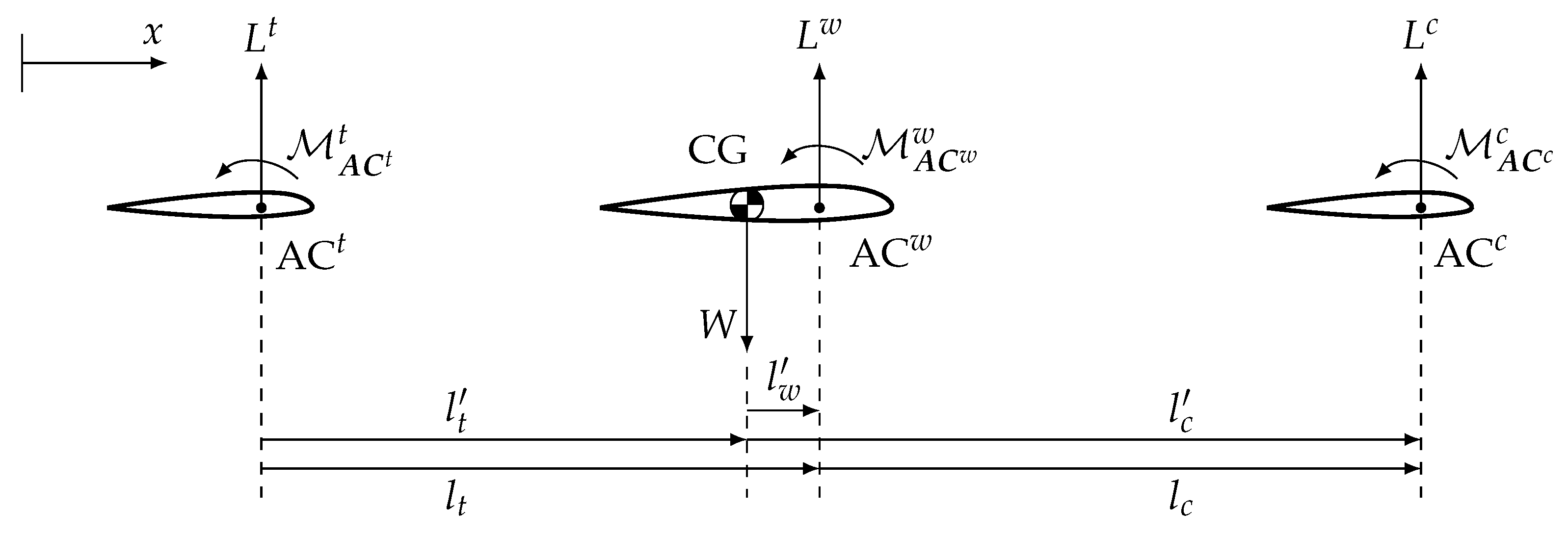Consider a steady flight condition along a straight horizontal trajectory, at a specific altitude with air density $\rho$ and speed V. In such flight regime, the vertical and pitching rotation equilibrium can be written as

$$\left\{\begin{array}{cc}\hfill C_L^{*}=& C_{L_{\alpha }}\alpha +C_{L_{{\delta }_e}}{\delta }_e+C_{L_{{\delta }_c}}{\delta }_c+C_{L_0}\hfill \\ \hfill 0=& C_{{\mathcal{M}}_{{\mathit{CG}}_{\alpha }}}\alpha +C_{{\mathcal{M}}_{{\mathit{CG}}_{{\delta }_e}}}{\delta }_e+C_{{\mathcal{M}}_{{\mathit{CG}}_{{\delta }_c}}}{\delta }_c+C_{{\mathcal{M}}_{{\mathit{CG}}_0}}\hfill \end{array}\right.$$

(47)

where $C_L^{*}$ is the lift coefficient at trim

$$C_L^{*}=\frac{2W/S}{\rho V^2},$$

(48)

and W is the airplane weight.

For convenience, Equation (48) can be written as

$${\mathit{y}}^{*}=\mathit{X}\mathit{\theta }+{\mathit{y}}_{\mathit{0}},$$

(49)

where

$$\begin{array}{ccc}{\mathit{y}}^{*}={[C_L^{*},0]}^T,& {\mathit{y}}_{\mathit{0}}={[C_{L_0},C_{{\mathcal{M}}_{{\mathit{CG}}_0}}]}^T,& \mathit{X}=\left[\begin{array}{ccc}{C}_{L_{\alpha }}& C_{L_{{\delta }_e}}& C_{L_{{\delta }_c}}\\ C_{{\mathcal{M}}_{{\mathit{CG}}_{\alpha }}}& C_{{\mathcal{M}}_{{\mathit{CG}}_{{\delta }_e}}}& C_{{\mathcal{M}}_{{\mathit{CG}}_{{\delta }_c}}}\end{array}\right].\end{array}$$

(50)

Equation (47) represents a set of two equations with three unknowns, which actually shows the redundancy in the longitudinal control when it comes to finding the trim solution, i.e., one has an ideally infinite number of possibilities to satisfy both vertical and pitch moment equilibria with different triads $\{\alpha ,{\delta }_e,{\delta }_c\}$.

This indeterminacy can be exploited for optimizing a merit index connected to the specific flight regime at hand. Moreover, since the trim lift coefficient $C_L^{*}$ will be function of the airplane speed V and weight W, optimizing the control inputs, ${\delta }_e$ and ${\delta }_c$, will be possible for each speed and weight, as opposed to what happens for standard aircraft, which are optimally designed only for a single condition.

To show this concept, one may consider the set $\{\alpha ,{\delta }_e,{\delta }_c\}$ which minimizes the drag coefficient $C_D$, given a specific trim lift coefficient, $C_L^{*}$. The drag coefficient $C_D$ as a merit function represents a suitable choice for coping with the redundancy. In fact, for a specific speed and weight—hence, for a specific $C_L^{*}$—minimum drag is associated to maximum lift-to-drag ratio $C_L/C_D$, maximum power index $C_L^{3/2}/C_D$ and maximum index $C_L^{1/2}/C_D$, which are all conditions associated to optimal performance in cruise for jet and propeller airplanes [14] (Chapter 2).

From a practical standpoint, the problem at hand could be viewed as the one of finding the angle of attack $\alpha$ and the controls ${\delta }_c$ and ${\delta }_e$, grouped in vector ${\mathit{\theta }}_{\mathit{opt}}$, that, for each specific speed, are able to trim the aircraft and, at the same time, to minimize its drag.

The optimal trim problem is then formalized as

$$\begin{array}{cc}\hfill {\mathit{\theta }}_{\mathit{opt}}=& \arg \min \left(C_D\left(\mathit{\theta }\right)\right)\hfill \\ \hfill \mathrm{s}.\mathrm{t}.& {\mathit{y}}^{*}=\mathit{X}\mathit{\theta }+{\mathit{y}}_{\mathit{0}}\hfill \end{array}$$

(51)

where function $C_D\left(\mathit{\theta }\right)$ is given in Equation (26).

Solution of the constrained problem (51) can be found with an unconstrained minimization of a suitable cost function J where constraints are considered through the Lagrange multipliers. To this end, J is defined as

$$J^{(=)}A+{\mathit{B}}^T\mathit{\theta }+{\mathit{\theta }}^T\mathit{C}\mathit{\theta }+{\mathit{\lambda }}^T\left(\mathit{X}\mathit{\theta }+{\mathit{y}}_{\mathit{0}}-{\mathit{y}}^{*}\right)$$

(52)

where $\mathit{\lambda }={\{{\lambda }_1,{\lambda }_2\}}^T$ represents the array of the Lagrange multipliers.

Imposing null partial derivatives with respect to $\mathit{\theta }$ and $\mathit{\lambda }$, to find the minimum J, leads to the following system of two equations

$$\left\{\begin{array}{c}\frac{\partial j}{\partial \mathit{\theta }}=\mathit{B}+2\mathit{C}\mathit{\theta }+{\mathit{X}}^T\mathit{\lambda }=0\hfill \\ \frac{\partial j}{\partial \mathit{\lambda }}=\mathit{X}\mathit{\theta }+{\mathit{y}}_{\mathit{0}}-{\mathit{y}}^{*}=0,.\hfill \end{array}\right.$$

(53)

which admits the following solution for ${\mathit{\theta }}_{\mathit{opt}}$

$$\begin{array}{c}\hfill {\mathit{\theta }}_{\mathit{opt}}=\frac{1}{2}{\mathit{C}}^{-1}\left({\mathit{X}}^T{\left(\mathit{X}{\mathit{C}}^{-1}{\mathit{X}}^T\right)}^{-1}\mathit{X}{\mathit{C}}^{-1}-\mathit{I}\right)\mathit{B}-{\mathit{C}}^{-1}{\mathit{X}}^T{\left(\mathit{X}{\mathit{C}}^{-1}{\mathit{X}}^T\right)}^{-1}\left({\mathit{y}}_{\mathit{0}}-{\mathit{y}}^{*}\right).\end{array}$$

(54)

where I is the 3 × 3 identity matrix.

Equation (54) can be rearranged to separate a constant contribution ${\mathit{\theta }}_{\mathit{0}}$ and a coefficient which multiplies y*, as

$$\begin{array}{c}\hfill {\mathit{\theta }}_{\mathit{opt}}={\mathit{\theta }}_{\mathit{0}}+{\Theta }_{\mathit{1}}{\mathit{y}}^{*},\end{array}$$

(55)

where

$$\begin{array}{c}\hfill {\mathit{\theta }}_{\mathit{0}}=-\frac{1}{2}{\mathit{C}}^{-1}\mathit{B}-{\mathit{C}}^{-1}{\mathit{X}}^T{\left(\mathit{X}{\mathit{C}}^{-1}{\mathit{X}}^T\right)}^{-1}{\mathit{y}}_{\mathit{0}}+\frac{1}{2}{\mathit{C}}^{-1}{\mathit{X}}^T{\left(\mathit{X}{\mathit{C}}^{-1}{\mathit{X}}^T\right)}^{-1}\mathit{X}{\mathit{C}}^{-1}\mathit{B}\end{array}$$

(56)

and

$$\begin{array}{c}\hfill {\Theta }_{\mathit{1}}={\mathit{C}}^{-1}{\mathit{X}}^T{\left(\mathit{X}{\mathit{C}}^{-1}{\mathit{X}}^T\right)}^{-1}.\end{array}$$

(57)

Notice that, since the second column of ${\Theta }_{\mathit{1}}$ multiplies the null element of ${\mathit{y}}^{*}$, vector ${\mathit{\theta }}_{\mathit{opt}}$ may be expressed directly as a linear function of the trim lift coefficient $C_L^{*}$, as

$${\mathit{\theta }}_{\mathit{opt}}={\mathit{\theta }}_{\mathit{0}}+\gamma C_L^{*},$$

(58)

where $\gamma ={[{\gamma }_{\alpha },{\gamma }_{{\delta }_e},{\gamma }_{{\delta }_c}]}^T$ is the first column of ${\Theta }_{\mathit{1}}$. Equation (58) demonstrates that there exists a simple linear relationship between the trim lift $C_L^{*}$ and the variables $\alpha$, ${\delta }_e$ and ${\delta }_c$, which allows for the minimization of the overall drag while trimming the aircraft. Furthermore, since Equation (54) is of general validity, we can expect that coefficients ${\mathit{\theta }}_{\mathit{0}}$ and $\gamma$ will be different for different aircraft configurations (e.g., different positions of the center of gravity) and flight regimes (e.g., passing from subsonic to transonic flight). However, as long as we consider linear aerodynamics and a quadratic drag polar, the optimal trim variables will be easily described as linear functions of the lift coefficient $C_L^{*}$.

Finally, due to the linearity of all trim variables with respect to $C_L^{*}$, it is possible to find a linear dependency between the deflection of the canard tail elevator for minimal drag.

To show this, first expand Equation (58) for each scalar variable in ${\mathit{\theta }}_{\mathit{opt}}$,

$$\left\{\begin{array}{c}{\alpha }_{opt}={\alpha }_0+{\gamma }_{\alpha }{C}_L^{*}\hfill \\ {\delta }_{e_{opt}}={{\delta }_e}_0+{\gamma }_{{\delta }_e}{C}_L^{*}\hfill \\ {\delta }_{c_{opt}}={{\delta }_c}_0+{\gamma }_{{\delta }_c}{C}_L^{*}.\hfill \end{array}\right.$$

(59)

with ${\alpha }_0$, ${{\delta }_e}_0$ and ${{\delta }_c}_0$, respectively the first, second and third elements of ${\mathit{\theta }}_{\mathit{0}}$. The last two lines of Equation (59) can be used to derive the relationship between the deflection of the two control surfaces as

$${\delta }_c={{\delta }_c}_0+\frac{{\gamma }_{{\delta }_c}}{{\gamma }_{{\delta }_e}}\left({\delta }_e-{{\delta }_e}_0\right)=q_{\delta }+r_{\delta }{\delta }_e,$$

(60)

with $r_{\delta }={\gamma }_{{\delta }_c}/{\gamma }_{{\delta }_e}$ and $q_{\delta }={{\delta }_c}_0-({\gamma }_{{\delta }_c}/{\gamma }_{{\delta }_e}){{\delta }_e}_0$.

As a final remark, inserting the optimal values for $\alpha$, ${\delta }_e$ and ${\delta }_c$ of Equation (59) into the expression of the drag coefficient in Equation (24), an expression of the optimal trimmed polar is readily obtained, which may be used for flight mechanics performance evaluation.

3.2. Optimization of Three-Surface Configuration for Maximum Lift-To-Drag Ratio

In this paragraph, the potential benefit of the three-surface configuration with redundant control on flight mechanics performance will be illustrated. In particular, a revision of the configuration of an existing two-surface aircraft will be considered, transforming it into a three-surface one, through the addition of a canard equipped with a movable surface. The final aim of this part is to assess the possibility to find a three-surface version of a standard two-surface aircraft with an improved lift-to-drag ratio.

From a technical standpoint, although limited, such an approach has the advantage of providing an indication of the goodness of the three-surface concept without requiring a complete design process—itself an activity of interest, which however falls outside of the scope of the present paper.

In fact, when thinking of the longitudinal configuration of a brand-new three-surface aircraft, in order to satisfy stringent performance, stability and maneuverability requirements, one should define, for a given fuselage, the values of six variables, e.g., the sizes of canard, tail and wing, $S^c$, $S^t$ and S, and the related location of their aerodynamic centers $x_{{\mathit{AC}}^t}$, $x_{{\mathit{AC}}^c}$ and $x_{{\mathit{AC}}^w}$. On the other hand, as it will be shown in the rest of this paragraph, when formulating the problem as an update of an existing two-surface airplane, one may introduce some constraints, which are necessary to primarily ensure that any new aircraft configuration share with the nominal one the same performance, and secondarily to limit the number of design parameters, and make the analysis easier to manage.

In accordance with the previous discussion, the wing area S was kept fixed to its nominal value. Furthermore, in order to provide for an airplane with similar stability and maneuvering characteristics, the static margin, defined in Equation (32), and the total empennage volume ${\overline{V}}_{tot}$, defined as the sum of the volumes of the tail and canard, ${\overline{V}}_{tot}={\overline{V}}^c+{\overline{V}}^t$, were kept constant. Moreover, the position of the third surface to be added to the nominal (two-surface) airplane is constrained by the length of the fuselage. Accordingly, the canard surface was placed in the farthermost forward position, which is expected to entail the best stability and maneuverability performance thanks to the beneficial impact of a higher moment arm. Based on a similar argument, the tail location is kept frozen and equal to that of the nominal airplane.

Dealing with the balance between degrees of freedom and constraints, after fixing the wing area and the location of tail and canard, and imposing the equality of the static margin and the total empennage volume between updated (three-surface) and nominal (two-surface) aircraft, the sizing problem results characterized by a single degree of freedom to be chosen among variables $S^t$, $S^c$ and $x_{{\mathit{AC}}^w}$. The canard surface $S^c$ is here selected as the optimization parameter.

For the sake of clarity, in the present work, the optimal three-surface configuration was found through a simple sensitivity analysis in which different canard surfaces are considered, rather than via a full optimization problem. Accordingly, the following approach was adopted to update the aircraft configuration. Given a specific value for $S^c$, in order to satisfy the total tail volume and static margin constraints, both the size of the tail $S^t$ and the position of the aerodynamic center of the main wing $x_{{\mathit{AC}}^w}$ are altered solving the following nonlinear problem

$$\begin{array}{cc}\hfill \mathrm{for}\mathrm{a}\mathrm{given}{S}^c,& \mathrm{find}\{S^t,x_{{\mathit{AC}}^w}\}\hfill \\ \hfill \mathrm{s}.\mathrm{t}.& {\overline{V}}_{tot}(S^c,S^t,x_{{\mathit{AC}}^w})={\overline{V}}_{to{t}_{\mathrm{nom}}}\hfill \\ \hfill & \mathrm{S}.\mathrm{M}.(S^c,S^t,x_{{\mathit{AC}}^w})=\mathrm{S}.\mathrm{M}{.}_{\mathrm{nom}}\hfill \end{array}$$

(61)

where ${\overline{V}}_{to{t}_{\mathrm{nom}}}$ and $\mathrm{S}.\mathrm{M}{.}_{\mathrm{nom}}$ are respectively the total empennage volume and the static margin of the nominal airplane.

Notice that, in this framework, we are including also the standard back-tailed airplane, corresponding to the nominal airplane, i.e., when $S^c=0$, and a canard version with same static margin and canard volume, in case $S^t=0$—which is obtained through a specific setting of $S^c$, to be better defined next. In between these two cases, we have all possible three-surface configurations, characterized again by the same total tail volume and static margin.

Obviously, the addition of the new forward surface, along with the modification in the tail size and wing location, generates also a change in the position of the aircraft center of gravity, which is to be taken into account. To this end, in any iteration of the solution of problem (61), the actual position of the aircraft center of gravity $x_{\mathrm{CG}}$ is computed as

$$x_{\mathrm{CG}}=\frac{m_{\mathrm{nom}}{x_{\mathrm{CG}}}_{\mathrm{nom}}-m^w\left(x_{{\mathrm{CG}}^w}-{x_{{\mathrm{CG}}^w}}_{\mathrm{nom}}\right)+\Delta m^t{x}_{{\mathrm{CG}}^t}+\Delta m^c{x}_{{\mathrm{CG}}^c}}{m_{\mathrm{nom}}+\Delta m^t+\Delta m^c},$$

(62)

where $m_{\mathrm{nom}}$ is the total mass of the nominal aircraft, while $m^w$ the mass of the wing, $x_{{\mathrm{CG}}^w}$ and ${x_{{\mathrm{CG}}^w}}_{\mathrm{nom}}$ are respectively the locations of the center of gravity of the actual and nominal wing, $x_{{\mathrm{CG}}^t}$ and $x_{{\mathrm{CG}}^c}$ are the locations of the center of gravity of tail and canard. Finally, $\Delta m^t$ and $\Delta m^c$ are the differences in the actual mass of tail and canard with respect to the nominal ones, which are estimated exploiting the Torenbeek method reported in Roskam [15] (Part V, Chapter 5), which relates the empennage mass with its own surface, as

$$W_{\mathrm{emp}}=K_h{S}_{\mathrm{emp}}\frac{3.81S_{\mathrm{emp}}^{0.2}{V}_D}{1000\sqrt{\cos \Lambda }}$$

(63)

where $W_{\mathrm{emp}}$ and $S_{\mathrm{emp}}$ are the weight in ${\mathrm{lb}}_{\mathrm{f}}$ and the area in ${\mathrm{ft}}^2$ of the empennage, $V_D$ the reference dive speed in $\mathrm{kn}$ and $K_h$ a coefficient equal to 1.0 or 1.1 respectively for fixed- or variable-incidence empennage.

Given a specific canard surface, the solution of problem (61) yields a new configuration of an equivalent three-surface airplane, featuring a trimmed polar which can be computed employing the optimization method described in Section 3.1. Clearly, for two-surface back-tailed and canard configurations, the trimmed polar is obtained following the standard methodology [16].

3.3. Updating a Twin-Engine, Two-Surface, Propeller Driven Airplane into an Optimal Three-Surface One

In this paragraph, the reconfiguration process explained in Section 3.2 will be applied to an aircraft model loosely based on the Diamond DA42 Twin Star, hereafter called nominal aircraft. The main characteristics of this nominal model are reported in

Table 1. Main characteristics of the nominal aircraft model, loosely based on the Diamond DA42 Twin Star. Longitudinal axis is pointing forward and has origin in the aerodynamic center of the tail.

Variable	Value	Unit of Measure
Aircraft mass, m	2000	$\mathrm{kg}$
Wing mass, $m^w$	571.5	$\mathrm{kg}$
Tail mass, $m^t$	20.0	$\mathrm{kg}$
Wing area, S	16.29	${\mathrm{m}}^2$
Tail area, $S^t$	2.35	${\mathrm{m}}^2$
Wing mean aerodynamic chord $\overline{c}$	1.1	$\mathrm{m}$
Tail mean aerodynamic chord ${\overline{c}}^t$	0.55	$\mathrm{m}$
Wing position, $x_{A{C}^w}$	4.6	$\mathrm{m}$
Maximum forward fuselage extension	7.35	$\mathrm{m}$
Nominal center of gravity position, $x_{CG}$	4.11	$\mathrm{m}$
Wing Oswald’s efficiency factor, $e^w$	0.8265	-
Tail Oswald’s efficiency factor, $e^t$	0.75	-
Wing incidence, $i^w$	0	$\mathrm{deg}$
Tail incidence, $i^w$	−1.1	$\mathrm{deg}$
Slope of wing lift curve, $C_{L_{\alpha }}^w$	0.0585	$1/\mathrm{deg}$
Slope of tail lift curve, $C_{L_{\alpha }}^t$	0.0775	$1/\mathrm{deg}$
Tail lift-to-elevator derivative, $C_{L_{{\delta }_e}}^t$	0.051	$1/\mathrm{deg}$
Constant drag coefficient of wing-body, $C_{D_0}^w$	0.03	-
Constant drag coefficient of tail, $C_{D_0}^t$	0.01	-
Wing aspect ratio, ${\lambda }^w$	11.06	-
Tail aspect ratio, ${\lambda }^t$	3.7	-
Wing pitching moment coefficient, $C_{{\mathcal{M}}_{{\mathit{AC}}^w}}$	−0.03	-
Tail pitching moment coefficient, $C_{{\mathcal{M}}_{{\mathit{AC}}^t}}$	−0.02	-
Constant downwash angle at tail, ${\epsilon }_{D_0}$	0.0	$\mathrm{deg}$
Derivative of downwash angle respect $\alpha$ at tail, ${\epsilon }_{D_{{\alpha }^w}}$	0.33	-

. Aerodynamic coefficients were computed based on [17].

Different equivalent aircraft were generated adding a canard lifting surface with $S^c\in \{0,2.38\}\left[\mathrm{m}\right]$ at a location corresponding to fuselage maximum forward extension. For each new configuration, the size of the tail $S^t$ and the location of the wing $x_{{\mathit{AC}}^w}$ were altered so as to maintain the same static margin and the same total tail volume of the nominal aircraft, as described by the constraints formulated in Section 3.2. The extreme values of the range of $S^c$ refer respectively to the nominal configuration, for $S^c=0$, and to an equivalent two-surface canard airplane, for $S^c=2.38{\mathrm{m}}^2$, which resulted associated to null $S^t$, given the data of the nominal aircraft and the problem constraints in Equation (61).

The characteristics of the canard surface common to all considered three-surface configurations are reported in

Table 2. Characteristics of the canard surface common to all considered three-surface configurations.

Canard-Related Variable	Value	Unit of Measure
Slope of canard lift curve, $C_{L_{\alpha }}^c$	0.098	$1/\mathrm{deg}$
Lift-to-elevator derivative, $C_{L_{{\delta }_c}}^c$	0.0654	$1/\mathrm{deg}$
Incidence, $i^c$	0	$\mathrm{deg}$
Constant drag coefficient, $C_{D_0}^c$	0.01	-
Oswald’s efficiency factor, $e^c$	0.85	-
Aspect ratio, ${\lambda }^c$	5.5	-
Pitching moment coefficient, $C_{{\mathcal{M}}_{{\mathit{AC}}^c}}$	−0.02	-
Constant downwash angle at wing, ${\epsilon }_{C_0}$	0.0	$\mathrm{deg}$
Derivative wrt. $\alpha$ of downwash angle at wing, ${\epsilon }_{C_{{\alpha }^c}}$	0.02	-
Derivative wrt. ${\delta }_c$ of downwash angle at wing, ${\epsilon }_{C_{{\delta }_c}}$	0.01	-
Wing-induced constant upwash, ${\epsilon }_{U_0}$	0.0	$\mathrm{deg}$
Derivative wrt. $\alpha$ of wing-induced upwash, ${\epsilon }_{U_{{\alpha }^w}}$	0.001	-

.

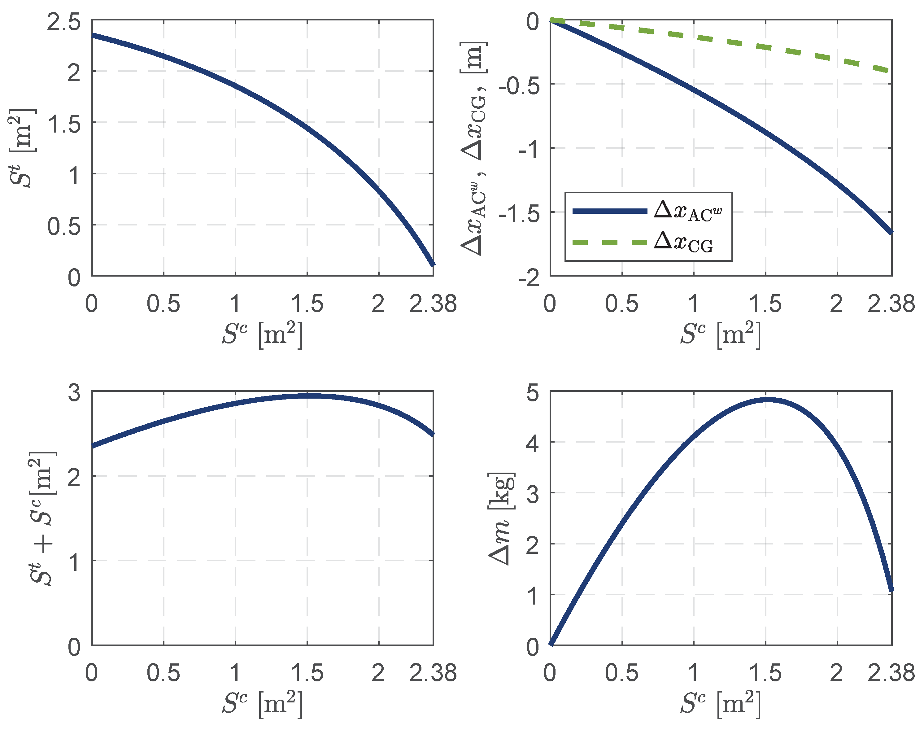
Figure 3 shows as functions of the canard surface $S^c$ some characteristics of the updated three-surface aircraft. The variation of the tail size and wing location are displayed respectively in the top-left and top-right plot. The top-right plot reports also the change of the airplane center of gravity, induced by the alteration of the wing position and the modification of the area of tail and canard. The bottom-left plot shows the total area of the empennages, while the bottom-right plot refers to the addition of the mass $\Delta m$ resulting from the generation of the equivalent new configurations.

Notice how the location of the wing moves backward as the canard surface increases to compensate for the destabilizing effect of the canard itself. This happens because the sensitivity of the neutral point with respect to the wing position is higher than that of the center of gravity. A mild increase in the total area of the empennages, sum of that of tail and canard, is experienced due to the introduction of the third lifting surface. This effect results from the fact that canard and tail are not equally distant from the aerodynamic center of the wing. Therefore, to impose the constraint on the total volume of the empennages, an increase in the canard area is associated to a tail area reduction of a lower magnitude, which eventually leads to an increase in the total mass. However, from the bottom-right plot in Figure 3, the latter appears negligible with respect to the total weight of the airplane.

As a remark, it can be observed that based on the assumed aspect ratio of the canard (Table 2, yielding a value of ${\lambda }^c=$ 5.5), the corresponding values of the canard span can be computed from Figure 3. This allows to accurately compare the canard span to the distance between the canard and wing aerodynamic centers. For instance, for a value of $S^c=$ 1.2 m${}^2$, this comparison yields a ratio of about 2.6 between the distance of the aerodynamic centers and the canard span, which is in good accordance with the hypothesis required for decoupling (as previously mentioned, a ratio greater than 1). For the top considered value of the canard surface (about $S^c=$ 2.38 m${}^2$), this ratio is equal to 2.4, showing that the aforementioned hypothesis on aerodynamics decoupling holds through all considered values of canard surface.

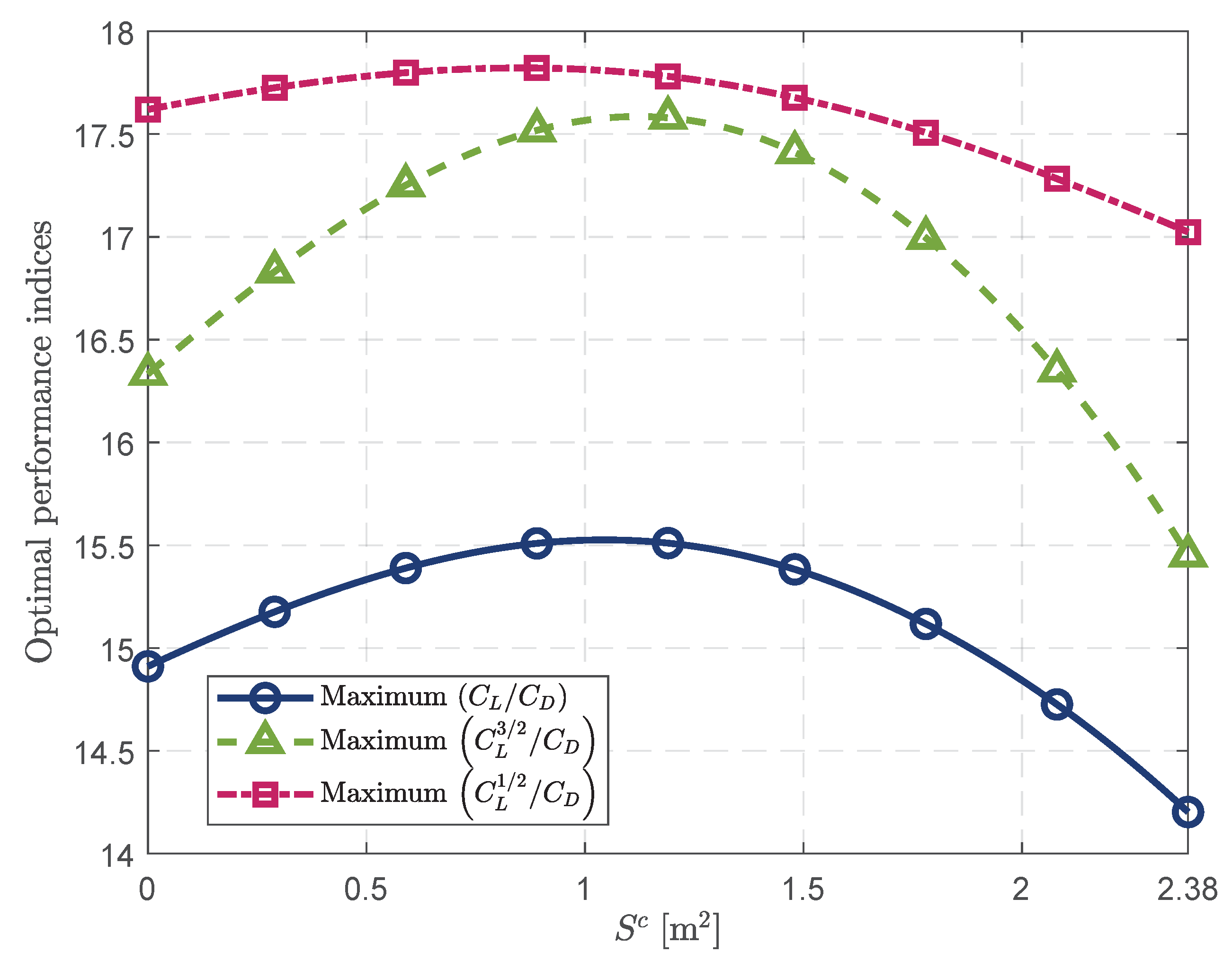
A relevant result of this analysis is reported in Figure 4, which shows the maximum achievable performance indices as function of the different configurations of three-surface airplane for variable canard areas. The maximum lift-to-drag ratio $C_L/C_D$, maximum power index $C_L^{3/2}/C_D$ and maximum $C_L^{1/2}/C_D$ were chosen as indicators for assessing the best possible airplane configuration among traditional back-tailed, canard and three-surface ones.

Both lift-to-drag ratio $C_L/C_D$ and power index $C_L^{3/2}/C_D$ are measures of performance of paramount importance for cruise of a prop-driven airplane, with ideally constant BSFC (Brake Specific Fuel Consumption), for which the maximum range and maximum endurance are respectively proportional to the maximum $C_L/C_D$ and to the maximum $C_L^{3/2}/C_D$ [14] (Chapter 2). It turns out that any increment in the values of such indices will lead to improved cruise performance, either in terms of range and endurance, or through a reduction of fuel consumption.

From the plot, it can be clearly noticed that a three-surface configuration with $S^c$ of about $1.2$${\mathrm{m}}^2$ is associated to the maximum values of the optimal indices for both performance indices, with an increase of about 4.0% in the maximum lift-to-drag ratio and about 7.6% in the power index.

Firstly, this fact demonstrates that it is possible to obtain an airplane with improved performance thanks to the addition of a third lifting surface with redundant longitudinal control. The expected gains are non-negligible, and may be worth the additional complexity entailed by such configuration.

Secondarily, since the update process is applied to an existing aircraft, it is reasonable to expect that a full redesign, which might consider also the size of the main wing as an optimization parameter, could in principle lead to more significant improvements. For example, with reference to the plots in Figure 3 one may immediately see that the optimal canard area $S^c$ is associated to a tail area of about 1.7 ${\mathrm{m}}^2$ and to an increment of the total empennage area $S^t+S^c$ of about 0.54 ${\mathrm{m}}^2$. Consequently, in order to compensate for such increment, one may imagine to reduce of the same entity the area of the main wing with a potential beneficial impact on weight, drag and size of the entire airplane.

Thirdly, looking again at Figure 3, the optimal configuration is associated to an increase of the total mass of the airplane of less than 5 $\mathrm{kg}$, which appears negligible given the mass of the nominal airplane, as already remarked. Clearly, that increment is related to the balance between the addition of a canard surface, as well as a reduction of the tail area. Other effects on the overall mass of the aircraft, potentially linked to the appearance of a new aerodynamic surface (like further control links), have not been accounted for at this level.

Fourthly, due to limited size of the canard, it is even reasonable to envision that the optimal three-surface configuration might not impact dramatically on the fuselage design and on its weight. In fact, the possible weight increment due to the addition of structural reinforcements in correspondence of the canard may be compensated by a lightening in the aft fuselage as a consequence of the smaller tail. Hence, although this should be verified with a detail design, a strong penalization in terms of fuselage structures and weight is not to be expected.

Figure 4 shows also the maximum $C_L^{1/2}/C_D$ index as a function of $S^c$. Clearly, such index is relevant only for jet airplanes with ideally constant TSFC (Thrust Specific Fuel Consumption), featuring the optimal range in the very correspondence of the maximum of that index. Hence, it may be of limited interest for the case considered in this paper. However, the plot reveals a potential gain of about 1.1% also for that index, for $S^c=0.9{\mathrm{m}}^2$. That area is slightly smaller than that obtained for optimal lift-to-drag ratio and power index. This finding suggests that the redundant control may be beneficial also for different types of airplane with respect to the one analyzed here. Moreover, since optimal performance indices may be obtained for different canard sizes, it is thought that a compromise choice will have to be done, when it will come to the full design or re-design of a new airplane on the basis of the relative importance that indices $C_L/C_D$, $C_L^{3/2}/C_D$ or $C_L^{1/2}/C_D$ have in accordance with the airplane mission.

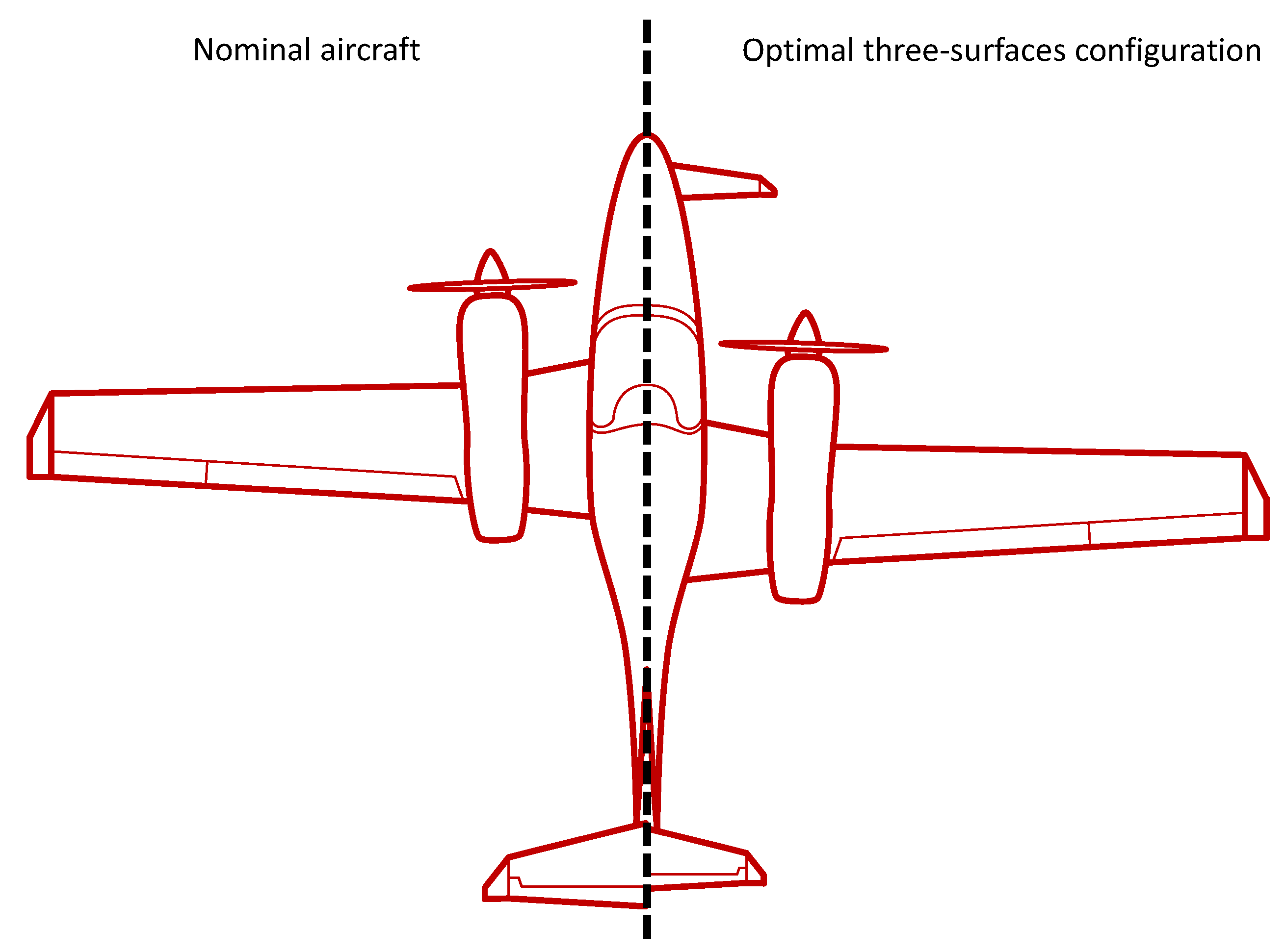
Finally, Figure 5 proposes a comparison in the appearance of the three-surface modified airplane for optimal lift-to-drag ratio and power index (right part) and the nominal one (left part). Through the sketch, the main changes in the configuration, i.e., the addition of the third surface, the subsequent reduction of the tail area and the backward shift of the main wing, are easily detectable. Both airplanes have similar mass, the same total empennage volume and the same static margin, but the updated one is characterized by a lift-to-drag ratio increased of about 4.0%, and power index of about 7.6%.

4. Flying Qualities and Control of a Three-Surface Aircraft: Assessment and Applications

In this section two studies will be presented, making use of the model for flight dynamics of the three-surface aircraft introduced in Section 2.2. In a first one, a control system will be proposed and tuned, aiming to make the three-surface aircraft perform in a similar way to a classical back-tailed, two-surface aircraft. A pole-placement design approach will be employed in this application. In a second study, a linear-quadratic regulator (LQR) will be designed to control the three-surface aircraft, allowing an investigation of an optimal use of the control surfaces in cruise, in turn suggesting how to better exploit some specific characteristics of the three-surface architecture for control.

4.1. Emulating the Dynamics of a Back-Tailed Aircraft with a Three-Surface Aircraft via Automatic Control

The increased number of controls on a three- surface aircraft, while allowing for the achievement of optimal cruise control (see Section 3), produces a greater control complexity in the longitudinal plane, compared to back-tailed two-surface aircraft. However, a purpose-designed control system may not only allow to condition the dynamics of the aircraft to match flying qualities acceptability criteria on eigenmodes, but when properly tuned, it might allow reproducing the response of a two-surface aircraft. This feature may be useful for easing pilot’s transition to a three-surface machine, making dynamic reaction of the three-surface aircraft in the longitudinal plane very similar to that of a standard back-tailed two-surface one.

4.1.1. Control Scheme A

A first control scheme proposed here for the task, and referred to as Scheme A in the following, is presented in Figure 6.

Working in a linearized framework, the corresponding dynamic equations include the linearized dynamics of the aircraft, introduced in Equation (33), and populated according to the extensive discussion in Section 2.2. Rearranged in state-space form, through the definitions of matrices ${\mathit{A}}_{LON}=-{\mathit{M}}_{LON}^{-1}{\mathit{K}}_{LON}$ and ${\mathit{B}}_{LON}=-{\mathit{M}}_{LON}^{-1}{\mathit{U}}_{LON}$, it yields Equation (64a), where the state and control vectors have been defined in Equation (34).

Measurement filters, required to wipe out turbulence and generally high-frequency disturbances in the measurements, will be associated to corresponding first order dynamics, reported in Equations (64b)–(64e).

The action of proportional controllers on the filtered control measures is associated to further dynamics, as per Equations (64f) and (64g). Finally, the closed-loop input variables for the canard and tail elevator controls, $u_c$ and $u_e$, are defined through Equations (64h) and (64i).

$$\begin{array}{cc}\hfill {\dot{\mathit{x}}}_{LON}& ={\mathit{A}}_{LON}{\mathit{x}}_{LON}+{\mathit{B}}_{LON}{\mathit{u}}_{LON}\hfill \end{array}$$

(64a)

$$\begin{array}{cc}\hfill {\dot{u}}_F& =-\frac{1}{{\tau }_{u_F}}\left(u_F-u\right)\hfill \end{array}$$

(64b)

$$\begin{array}{cc}\hfill \Delta {\dot{\alpha }}_F& =-\frac{1}{{\tau }_{{\alpha }_F}}\left(\Delta {\alpha }_F-\Delta \alpha \right)\hfill \end{array}$$

(64c)

$$\begin{array}{cc}\hfill \Delta {\dot{q}}_F& =-\frac{1}{{\tau }_{q_F}}\left(\Delta q_F-\Delta q\right)\hfill \end{array}$$

(64d)

$$\begin{array}{cc}\hfill \Delta {\dot{\theta }}_F& =-\frac{1}{{\tau }_{{\theta }_F}}\left(\Delta {\theta }_F-\Delta \theta \right)\hfill \end{array}$$

(64e)

$$\begin{array}{cc}\hfill \Delta \dot{{\delta }_e}& =-\frac{1}{{\tau }_{{\delta }_e}}\left(\Delta {\delta }_e-u_e\right)\hfill \end{array}$$

(64f)

$$\begin{array}{cc}\hfill \Delta \dot{{\delta }_c}& =-\frac{1}{{\tau }_{{\delta }_c}}\left(\Delta {\delta }_c-u_c\right)\hfill \end{array}$$

(64g)

$$\begin{array}{cc}\hfill u_e& ={\delta }_{e_{pilot}}-k_{u_e}{u}_F-k_{{\alpha }_e}\Delta {\alpha }_F-k_{q_e}\Delta q_F-k_{{\theta }_e}\Delta {\theta }_F\hfill \end{array}$$

(64h)

$$\begin{array}{cc}\hfill u_c& ={\delta }_{c_{pilot}}-k_{u_c}{u}_F-k_{{\alpha }_c}\Delta {\alpha }_F-k_{q_c}\Delta q_F-k_{{\theta }_c}\Delta {\theta }_F.\hfill \end{array}$$

(64i)

It is noteworthy that, apart from $\alpha$ which might require in practice some sophistication in the design of the sensor chain, all measurements are standarly obtained via gyros, inertial units and air data measurement systems.

4.1.2. Results of Dynamics Reassignment with Scheme A

Considering the same optimal three-surface testbed introduced in Section 3.3, obtained through an update of the Diamond DA-42, with a suitable tuning of the gains in Equation (64), it is possible to re-obtain the dynamics of the standard two-surface aircraft.

In the following comparison in Figure 7, the eigenvalues corresponding to the short period and phugoid modes are presented on the left and right plots respectively. The free response of the two-surface nominal aircraft is represented by triangles, whereas the free response of the updated optimal three-surface aircraft is represented by circles. Finally, crosses correspond to the re-assigned dynamics of the three-surface aircraft. Ideally, the latter should coincide with triangles, representing a match between the controlled dynamics of the three-surface and the free response of the two-surface aircraft. The reference flight Mach for linearization is $Ma=0.28$.

A pole-placement technique is used to design the gains in the control scheme introduced in Figure 6.

As it can be seen from the plots in Figure 7, where for short period a very good correspondence is achieved between the conditioned dynamics of the three-surface aircraft and the two-surface baseline, the corresponding phugoid is less accurately placed with respect to the target.

4.1.3. Control Scheme B

A second control scheme, referred to as Scheme B in the following, is based on the same baseline of Scheme A, with the feedback of two measures of elevator deflections $\Delta {\delta }_c$ and $\Delta {\delta }_e$. These are typically obtainable from sensor readings in the control chain. Scheme B is presented in Figure 8.

Correspondingly, the associated dynamic equations in Equation (64) are augmented by

$$\begin{array}{cc}\hfill \Delta {\dot{{\delta }_e}}_F& =-\frac{1}{{\tau }_{{{\delta }_e}_F}}\left(\Delta {\delta }_{e_F}-\Delta {\delta }_e\right)\hfill \end{array}$$

(65a)

$$\begin{array}{cc}\hfill \Delta {\dot{{\delta }_c}}_F& =-\frac{1}{{\tau }_{{{\delta }_e}_F}}\left(\Delta {\delta }_{c_F}-\Delta {\delta }_c\right),\hfill \end{array}$$

(65b)

and Equations (64h) and (64i), strictly referring to Scheme A, are substituted by Equation (66) from the flowchart of Scheme B, yielding

$$\begin{array}{cc}\hfill u_e& ={\delta }_{e_{pilot}}-k_{u_e}{u}_F-k_{{\alpha }_e}\Delta {\alpha }_F-k_{q_e}\Delta q_F-k_{{\theta }_e}\Delta {\theta }_F-k_{{\delta }_e}^e\Delta {\delta }_{e_F}-k_{{\delta }_c}^e\Delta {\delta }_{c_F}\hfill \end{array}$$

(66a)

$$\begin{array}{cc}\hfill u_c& ={\delta }_{c_{pilot}}-k_{u_c}{u}_F-k_{{\alpha }_c}\Delta {\alpha }_F-k_{q_c}\Delta q_F-k_{{\theta }_c}\Delta {\theta }_F-k_{{\delta }_c}^e\Delta {\delta }_{e_F}-k_{{\delta }_c}^c\Delta {\delta }_{c_F}.\hfill \end{array}$$

(66b)

4.1.4. Results of Dynamics Reassignment with Scheme B

A comparison qualitatively similar to Figure 7, is presented in Figure 9, where the left plot refers again to short period and the right one to phugoid. The reference flight Mach for linearization is $Ma=0.28$, equal to the value considered in Section 4.1.2.

By comparison with Figure 7, results in Figure 9 are clearly better, not only providing a good match in resembling the short period dynamics of the nominal aircraft with the controlled three-surface, but also allowing for a better accuracy on phugoid.

With this control scheme, it can be argued that the same longitudinal dynamics of a two-surface aircraft can be obtained on a conditioned three-surface aircraft, re-designed under the constraints and with the optimal cruise objective presented in Section 3.2. This ensures that a similar meneuvering flight performance may be achieved, despite the addition of a new surface, by means of a rather low-technology, easily implementable control scheme.

4.2. Linear-Quadratic Regulator Law for Dynamics Stabilization on a Three-Surface Aircraft

The gains in the controllers presented in Section 4.1 have been tuned through a pole placement design scheme. A linear-quadratic regulator (LQR) makes for an alternative to that type of design, well suited for a multi-input, multi-output system for which the dynamics are assigned in a linear form, here represented by Equations (64a)–(64e), accounting also for filtering dynamics.

As known, among the advantages of the LQR control design technique is the knowledge of the complete dynamics of the system, which are entirely accounted for by the design, and the higher degree of automation achievable in the controller synthesis with respect to a pole placement procedure.

In order for the design procedure to be carried out, the covariance matrices $\mathit{Q}$ and $\mathit{R}$ of the states and controls respectively need to be assigned.

Results of LQR Control for Longitudinal Stabilization

An LQR controller has been designed based on state equation Equations (64a)–(64g), aimed at the stabilization of the free response of the optimal three-surface aircraft considered in the previous sections.

To the aim of stabilizing the system without incurring in non-realistic control histories, the following covariances have tested satisfactory,

$$\begin{array}{ccc}\mathit{Q}=\mathrm{diag}(0.01,0.1,0.1,0.01,0,0,0,0),& & \mathit{R}=\mathrm{diag}(100,10).\end{array}$$

(67)

The resulting plots for short period (left) and phugoid (right) modes are presented in Figure 10.

It can be noticed how the eigenvalues of the stabilized system are correctly shifted towards higher frequency and higher damping.

4.3. Comparison of Control Loads in Time Domain for Pole-Placement and Lqr Techniques

An insight provided by a suitable use of the model for a three-surface aircraft presented in this work is related to the different use of control inputs obtained from the adoption of a pole-placement—in particular, Scheme B, as seen in Section 4.1.3 and Section 4.1.4—or an LQR scheme—as seen in Section 4.2—for the reassignment of the dynamics of the aircraft.

Consider a scenario where the aircraft in steady horizontal flight is excited according to the time history of pilot’s control set-points displayed in Figure 11.

The response of the conditioned system for the two cases of pole placement and LQR can be analyzed computing in particular the body vertical and longitudinal control force components, as well as the pitching moment control component, which can be defined as follows

$$\begin{array}{cc}\hfill \Delta {C_Z}^{t,ctrl}& =C_{Z_{{\delta }_e}}\Delta {\delta }_e,\hfill \end{array}$$

(68a)

$$\begin{array}{cc}\hfill \Delta {C_Z}^{c,ctrl}& =C_{Z_{{\delta }_c}}\Delta {\delta }_c,\hfill \end{array}$$

(68b)

$$\begin{array}{cc}\hfill \Delta C_Z^{ctrl}& =\Delta {C_Z}^{t,ctrl}+\Delta {C_Z}^{c,ctrl},\hfill \end{array}$$

(68c)

$$\begin{array}{cc}\hfill \Delta C_{{\mathcal{M}}_{\mathit{CG}}}^{t,ctrl}& =C_{{\mathcal{M}}_{{\mathit{CG}}_{{\delta }_e}}}\Delta {\delta }_e,\hfill \end{array}$$

(68d)

$$\begin{array}{cc}\hfill \Delta C_{{\mathcal{M}}_{\mathit{CG}}}^{c,ctrl}& =C_{{\mathcal{M}}_{{\mathit{CG}}_{{\delta }_c}}}\Delta {\delta }_c,\hfill \end{array}$$

(68e)

$$\begin{array}{cc}\hfill \Delta C_{{\mathcal{M}}_{\mathit{CG}}}^{ctrl}& =\Delta C_{{\mathcal{M}}_{\mathit{CG}}}^{t,ctrl}+\Delta C_{{\mathcal{M}}_{\mathit{CG}}}^{c,ctrl},\hfill \end{array}$$

(68f)

where superscript ${(·)}^{ctrl}$ stands for control component.

Figure 12 displays on the plots to the left and right respectively the response of the three-surface aircraft considered in the previous sections, augmented by a conditioning controller designed on Scheme B (left) or an LQR approach (right). Considered time histories are those of controls, vertical control force coefficients and control pitching moment (respectively from top to bottom).

Looking at the control inputs (top row), following the neutralization of the control set-points at $t=3$ s according to Figure 11, the two controllers show an opposite behavior. Where the pole-placement designed control tends to push the controls in the same direction, with a limited phase shift, the LQR immediately pushes the controls in the opposite direction, moving them at a $\pi$ phase angle for the rest of the time history.

The ensuing control force behavior (mid row) features for the case of the pole-placement designed controller a canard and tail contribution producing an oscillating overall control force, whereas for the LQR the contributions of the two surfaces balance each other, leading to a lower oscillating, quickly decaying global control force. In turn, this results in a different control moment behavior (bottom row), where both controllers display an oscillating behavior, with the LQR decaying faster back to the equilibrium condition.

It might be argued that the LQR, through a better knowledge of the overall coupled behavior obtained through a design making use of the dynamics modeled as shown in Section 2, smartly acts on control forces to avoid any unbalance in the vertical force, and through a smart coordinated action on the canard and tail it achieves a more effective control through pitching moment only.

5. Conclusions and Outlook

In this paper, a three-surface aircraft with redundant longitudinal control is analyzed in order to understand whether such configuration can be an effective means for improving the flight mechanics performance of modern fleets. The three-surface configuration is realized using, in the same aircraft, both a horizontal tail and a canard wing respectively located in the aft and fore parts of the fuselage. More importantly, both empennages are equipped with a control input, i.e., a movable aerodynamic appendix, creating a redundancy in the longitudinal control of the aircraft.

Although there exists a multitude of aircraft with three lifting surfaces, i.e., the main wing, the horizontal tail and the canard, the possibility of using the third surface for hosting an additional degree of longitudinal control to optimize the trimmed polar was never the object of a systematic analysis.

With the aim of providing a mathematical framework for studying such aircraft already at a preliminary design phase, this paper started off by developing a steady and a dynamic flight mechanics models, including both tail and canard empennages along with their control degrees.

The steady mathematical model was then used for optimizing the three-surface configuration through a two-pronged approach.

Firstly, it was shown that the redundant control can be used for minimizing the trimmed drag coefficient for any trimmed lift coefficient, i.e., for any weight, altitude and speed of the aircraft, as opposed to traditional planes which are optimized only for a single condition. In particular, the solution of this minimization problem can be found in closed form and leads to a linear relationship between the canard and the tail deflection.

Secondarily, the problem of turning an existent traditional back-tailed aircraft into an equivalent three-surface version was considered. Many updated configurations were generated by adding a canard wing of variable size constraining the three-surface versions to have the same static margin and total empennage volume (i.e., the sum of canard and tail volume) of the nominal airplane. This led to modifications in the location of the wing and tail surfaces. It was then demonstrated that there exists a three-surface configuration associated to optimal values for the maximum lift-to-drag ratio $C_L/C_D$, maximum power index $C_L^{3/2}/C_D$ and maximum $C_L^{1/2}/C_D$, featuring gains with respect to the nominal airplane equal to 4.0%, 7.6% and 1.0% respectively. These promising results on the one hand demonstrate the possibility of improving the flight mechanics characteristics of an aircraft through an update to a three-surface configuration with redundant control, and on the other they show that such a configuration can be a valuable option to be considered in the preliminary phases of the airplane conceptual design. The improvements obtained as a result of the addition and proper sizing of a canard are preliminary, but they provide a meaningful proof of concept of the potential of a three-surface configuration with redundant control.

Finally, the dynamic model was used for quantifying the characteristics of the longitudinal modes and for synthesizing some automatic controls in the unusual case of the three-surface airplane with two longitudinal degrees of freedom. In a first exercise, it was demonstrated that through a simple state feed-back, it is possible to emulate the dynamics of the nominal aircraft with the updated configuration, via a pole-placement based control design.

In a second exercise, the optimal LQR (linear quadratic regulator) has been employed to increase the damping factors of short period and phugoid. From the obtained results, it seemed that, if left free to control the system, the optimal regulator acts on the two control degrees in counter-phase. This leads to a minimization of the imbalance in the vertical force produced by the couple tail-canard, generating this way a pure pitching moment which results more effective in damping out the oscillations in pitch. Note that this interesting feature can be obtained only with the double longitudinal empennage and the redundant control, characterizing the innovative configuration studied in this work.

In terms of possible improvements of this work, one should first analyze the proposed configuration for aircraft of different sizes and typology, e.g., jet liners, to possibly verify the consistency of the obtained results for heavier airplanes. Additionally, one may consider the full design of a three-surface aircraft to understand whether such a configuration may be further ameliorated thanks to a proper sizing of the wing, featuring a possible smaller area with a consequent lower drag.

In terms of possible extensions, it is certainly interesting to evaluate the possibility of improving the aircraft capabilities in cruise and terminal maneuvers thanks to the redundancy in the longitudinal control. For example, in principle, an imbalance between the lift and weight may be generated by a coordinated control of both canard and elevator deflections without an increase of the angle of attack and pitch. This fact could be exploited for both improving turning performance, and during the rotation phase within take-off, for decreasing take-off distance or reducing the required clearance between fuselage aft and tail, with a beneficial impact on landing gear size and weight.

References

1. Gundlach, J. Designing Unmanned Aircraft Systems: A Comprehensive Approach, 2nd ed.; American Institute of Aeronautics and Astronautics: Reston, VA, USA, 2012. [Google Scholar]
2. Agnew, J.; Hess, J. Benefits of aerodynamic interaction to the three-surface configuration. J. Aircr. 1980, 17, 823–827. [Google Scholar] [CrossRef]
3. Kendall, E.R. The minimum induced drag, longitudinal trim and static longitudinal stability of two-surface and three-surface airplanes. In Proceedings of the AIAA 2nd Applied Aerodynamics Conference, Seattle, WA, USA, 21–23 August 1984. [Google Scholar]
4. Kendall, E.R. The theoretical minimum of induced drag of three-surface airplanes in trim. J. Aircr. 1985, 22, 847–854. [Google Scholar] [CrossRef]
5. Kroo, I. A general approach to multiple lifting surface design and analysis. In Proceedings of the Aircraft Design Systems and Operations Meeting, San Diego, CA, USA, 31 October–2 November 1984. [Google Scholar]
6. Strohmeyer, D.; Seubert, R.; Heinze, W.; Osterheld, C.; Fornasier, L. Three surface aircraft—A concept for future transport aircraft. In Proceedings of the 38th AIAA Aerospace Science Meeting and Exhibit, Reno, NV, USA, 1–3 January 2000. [Google Scholar]
7. Ricci, S.; Scotti, A.; Zanotti, D. Control of an all-movable foreplane for a three surface aircraft wind tunnel model. Mech. Syst. Signal Process. 2006, 20, 1044–1066. [Google Scholar] [CrossRef]
8. Mattaboni, M.; Quaranta, G.; Mantegazza, P. Active flutter suppression for a three-surface transport aircraft by recurrent neural networks. J. Guid. Control Dyn. 2009, 32, 1295–1307. [Google Scholar] [CrossRef]
9. Riboldi, C.E.D.; Gualdoni, F. An integrated approach to the preliminary weight sizing of small electric aircraft. Aerosp. Sci. Technol. 2016, 58, 134–149. [Google Scholar] [CrossRef]
10. Riboldi, C.E.D. An optimal approach to the preliminary design of small hybrid-electric aircraft. Aerosp. Sci. Technol. 2018, 81, 14–31. [Google Scholar] [CrossRef]
11. Diamond Aircraft Industries GmbH N.A.-Otto Straße 5, 2700 Wiener Neustadt. Available online: https://www.diamondaircraft.com/en/about-diamond/why-diamond/locations/ (accessed on 7 May 2021).
12. Phillips, J.D. Approximate Neutral Point of a Subsonic Canard Aircraft; NASA Technical Memorandum 86694; NASA Ames Research Center: Moffett Field, CA, USA, 1985.
13. Levy, D. Prediction of average downwash gradient for canard configurations. In Proceedings of the 30th AIAA Aerospace Science Meeting and Exhibit, Reno, NV, USA, 6–9 January1992. [Google Scholar]
14. Pamadi, B.N. Performance, Stability, Dynamics and Control of Aircraft; American Institute of Aeronautics and Astronautics: Reston, VA, USA, 1998. [Google Scholar]
15. Roskam, J. Airplane Design; Roskam Aviation and Engineering Corporation: Ottawa, KS, USA, 1988. [Google Scholar]
16. Borri, M.; Trainelli, L. Airplane equilibrium and stability: A simplified teaching approach. In Proceedings of the 17th Congresso Nazionale AIDAA, Rome, Italy, 15–17 September 2003. [Google Scholar]
17. Gudmundsson, S. General Aviation Aircraft Design: Applied Methods and Procedures; Butterworth-Heinemann: Amsterdam, The Netherlands, 2014. [Google Scholar]
Figure 1. Three-surface model scheme for lift and pitching moment.
Aerospace 08 00139 g001
Figure 2. Definition of aerodynamic angles for all surfaces. ZLL stands for ’Zero-Lift Line’.
Aerospace 08 00139 g002
Figure 3. Tail surface (top-left), sum of tail and canard surface (bottom-left), variation in main wing location Δ x AC w and in center of gravity position Δ x CG (top-right) and increase in mass Δ m (bottom-right) as functions of the canard size S c . S c = 0 indicates the traditional two-surface back-tailed configuration. The black thin dashed line at S c = 2.38 refers to the two-surface canard configuration.
Aerospace 08 00139 g003
Figure 4. Maximum lift-to-drag ratio as function of the canard surface. Circle markers: analyzed configurations; solid line: spline interpolation.
Aerospace 08 00139 g004
Figure 5. Sketch of the nominal DA42 airplane (left) and optimal three-surface equivalent version (right).
Aerospace 08 00139 g005
Figure 6. Scheme A for dynamics reassignment of a three-surface aircraft.
Aerospace 08 00139 g006
Figure 7. Eigenvalues of short period (a) and phugoid (b) for the two-surface testbed (triangles), three-surface testbed (circles) and three-surface with re-assigned dynamics via Scheme A (crosses). Lines represent limits for Level 1 flying qualities (black lines: phugoid, blue lines: Category B short period, red lines: Category A short period.
Aerospace 08 00139 g007
Figure 8. Scheme B for dynamics reassignment of a three-surface aircraft.
Aerospace 08 00139 g008
Figure 9. Eigenvalues of short period (a) and phugoid (b) for the two-surface testbed (triangles), three-surface testbed (circles) and three-surface with reassigned dynamics (crosses) via Scheme B. Lines represent limits for Level 1 flying qualities (black lines: phugoid, blue lines: Category B short period, red lines: Category A short period.
Aerospace 08 00139 g009
Figure 10. Eigenvalues of short period (a) and phugoid (b) for the three-surface testbed (circles) and three-surface with reassigned dynamics (crosses) via LQR. Lines represent limits for Level 1 flying qualities (black lines: phugoid, blue lines: Category B short period, red lines: Category A short period.
Aerospace 08 00139 g010
Figure 11. Pilot control set-points δ e p i l o t and δ c p i l o t for response comparison.
Aerospace 08 00139 g011
Figure 12. Comparison of the time histories of controls (first row, a,b), vertical control force coefficient (mid row, c,d) and control pitching moment (bottom row, e,f), for a control set-point history as in Figure 11, for the three-surface testbed conditioned by a Scheme B, pole placement designed controller (left) and an LQR controller (right).
Aerospace 08 00139 g012