
PSO-Based Soft Lunar Landing with Hazard Avoidance: Analysis and Experimentation


1
School of Aerospace Engineering, Sapienza University of Rome, Via Salaria 851, 00138 Rome, Italy
2
Italian Space Agency, Via del Politecnico snc, 00133 Rome, Italy
*
Author to whom correspondence should be addressed.
Aerospace 2021, 8(7), 195; https://0-doi-org.brum.beds.ac.uk/10.3390/aerospace8070195
Submission received: 26 May 2021
/
Revised: 9 July 2021
/
Accepted: 15 July 2021
/
Published: 19 July 2021
Abstract
:The problem of real-time optimal guidance is extremely important for successful autonomous missions. In this paper, the last phases of autonomous lunar landing trajectories are addressed. The proposed guidance is based on the Particle Swarm Optimization, and the differential flatness approach, which is a subclass of the inverse dynamics technique. The trajectory is approximated by polynomials and the control policy is obtained in an analytical closed form solution, where boundary and dynamical constraints are a priori satisfied. Although this procedure leads to sub-optimal solutions, it results in beng fast and thus potentially suitable to be used for real-time purposes. Moreover, the presence of craters on the lunar terrain is considered; therefore, hazard detection and avoidance are also carried out. The proposed guidance is tested by Monte Carlo simulations to evaluate its performances and a robust procedure, made up of safe additional maneuvers, is introduced to counteract optimization failures and achieve soft landing. Finally, the whole procedure is tested through an experimental facility, consisting of a robotic manipulator, equipped with a camera, and a simulated lunar terrain. The results show the efficiency and reliability of the proposed guidance and its possible use for real-time sub-optimal trajectory generation within laboratory applications.
1. Introduction
In recent years, space agencies have experienced a renewed interest in lunar robotic missions. Indeed, China National Space Administration and Indian Space Research Organization are involved in the Chang’e [1,2,3] and the Chandrayaan [4,5] project respectively: both the projects are made up of multiple missions directed to the Moon which exploit orbiters, landers, rovers, and sample return spacecraft. Moreover, the Korea Aerospace Research Institute (South Korea) and Roscomos (Russia) are planning to explore the Moon thanks to the mission Korea Pathfinder Lunar Orbiter [6] and the program Luna [7]. Finally, many companies will also deliver technological demonstrators, landers, and rovers on the Moon (mostly in the south polar region) as contracts of NASA Commercial Lunar Payload Services (CLPS) program [8], with the goals of testing in situ resource utilization concepts, scouting for lunar resources, and delivering science and technology payloads to support the Artemis lunar program (https://www.nasa.gov/specials/artemis/, accessed on 16 July 2021).
As can be perceived from the aforementioned missions, robotic space exploration is essential to achieve all the mission objectives. In particular, automation is a crucial feature of such spacecraft, since it allows for obtain accurate, reliable, and safe maneuvers, such as those required for landing trajectories. Within this framework, it is necessary to have an onboard trajectory generation, for example in case of failure of the engines or lack of communication with the ground. Moreover, the presence of craters on the Moon requires an autonomous hazard avoidance [9], which allows for achieving the landing in a safe region outside craters. This means that a new trajectory should be planned as soon as one of the previous conditions occurs; the new guidance should also be optimal in terms of the minimum time or the minimum fuel consumption. This is actually the goal of this paper, i.e., to propose and test, with an experimental application, a sub-optimal guidance based on the well-known metaheuristic algorithm Particle Swarm Optimization (PSO) [10] and the inverse dynamics approach [11] for lunar landing trajectories.
Lunar landing trajectories have already been the objectives of many studies in literature. They have been studied by means of the circular guidance law and polynomials in Ref. [12]. Many other works consider optimal trajectories; for instance, multi-phase constrained fuel-optimal lunar landings have been obtained through a Legendre pseudospectral philosophy [13]. Legendre pseudospectral method is also considered in Ref. [14] together with Nonlinear Programming (NLP) to obtain fuel-optimal, two-dimensional soft lunar landing trajectories starting from a parking orbit. Optimal lunar landings have also been studied in [15], in which the authors have proposed a novel nonlinear spacecraft guidance scheme, based on the optimal sliding surface, utilizing a hybrid controller. Furthermore, propellant-optimal trajectories for a powered descent pinpoint lunar landing, based on the Pontryagin Maximum Principle (PMP), have also been obtained in Ref. [16] by means of a polynomial guidance law: in this work, the pinpoint soft landing problem is transformed into a Two Point Boundary Value Problem (TPBVP) solved by a NLP algorithm. Polynomial guidance is also exploited in Ref. [17], together with the inverse dynamics approach, to obtain fuel-optimal trajectories. Metaheuristic algorithms have also been used to study lunar landing optimal trajectories, as demonstrated by Ref. [18], in which the Ant Colony Optimization is used.
In addition, real-time optimal guidance is an open research field because of the difficulties in rapidly computing optimal trajectories. Based on the above considerations, this paper illustrates how it is possible to obtain a sub-optimal guidance for lunar landing trajectories with low computational times. This goal is reached by using the combination of two approaches. First, PSO is employed to ensure a fast optimal global search; its effectiveness and reliability within space guidance have already been proved and widely accepted in literature [19,20,21,22,23]. However, at the best of the authors’ knowledge, PSO has never been used to design real-time optimal trajectories for lunar landing to be used for laboratory’s experimental applications. Secondly, a particular subclass of inverse dynamics technique, called differential flatness [24,25], and polynomial approximation of the trajectory are exploited; this approach allows for overcoming some issues of direct dynamics, i.e., the integration of the dynamics equations is avoided, the dynamical constraints are a priori satisfied, the boundary conditions are directly fulfilled, and the control policy is obtained in an analytical closed form. This procedure causes the fast computation of the whole optimization process and consequently the possibility to generate fast optimal trajectories. It is important to highlight that the combination of the inverse dynamics approach, based on the polynomial approximation of the trajectory, and a basic version of the PSO actually allows for obtaining low computational times. Therefore, the software can be implemented on hardware to obtain sub-optimal trajectories for laboratory’s experimental simulations, as it is shown in this paper. The sub-optimality is due to the polynomial approximation of the trajectory; however, in general, computing fast and real-time optimal trajectories is always a compromise between the computational time and the optimality of the results. The proposed methodology is practically tested through an experimental facility represented by a simulated lunar terrain and a Cartesian robotic manipulator [26,27] equipped with a camera through which craters could be detected.
Furthermore, since a thruster that works in pulsed mode is considered, a Pulse Width Modulation (PWM) is actually employed to transform the continuous computed optimal control into the pulsed one, actually implemented. This can introduce some errors in the final target position and velocity, as will be explained in the next sections. Hence, to reduce the errors due to PWM and to counteract the possibility of failure of the PSO-based optimization (for example, if a feasible solution is not found because of the randomness or the not fulfilled control constraints), some additional (analytically computed) maneuvers are proposed to safely land at the expense of a greater flight time and amount of propellant. This results in a more robust trajectory planning. All the work presented in this paper represents the first step for future real-time testing on hardware that has already been tested for flight, such as FPGA [28].
This paper is organized as follows: Section 2 and Section 3 introduce the state of the art of autonomous trajectory planning, the experimental facility, and the environment of the lunar landing, including the equations of motion, the boundary, and control constraints. Section 4 describes the general guidance approach, based on PSO and inverse dynamics techniques together with the method to transform continuous into pulsed control acceleration. Moreover, hazard detection and avoidance techniques and the control proposed for the very last phase of the landing trajectory are discussed. Section 5 presents numerical and experimental results. Finally, concluding remarks are given in Section 6.
2. Autonomous Trajectory Planning Framework
The first part of this Section deals with some studies already developed in literature related to autonomous (real-time) trajectory planning, in order to highlight the importance of this topic and better understand the reasons behind the project the authors of this paper are working on. Afterwards, the experimental facility employed to test the autonomous trajectory planning algorithm, proposed in this work, is presented.
2.1. Related Works
This section focuses on some works related to real-time autonomous trajectory planning, whose aim is to increase the autonomy of the spacecraft in taking safe and reliable decisions without the need of the mission controllers to interfere. Until now, spacecraft independence is often limited and the maneuvers are usually computed offline and uploaded by ground control. Overall, this limits the mission flexibility and efficiency, impacting the capability.
Trajectory planning is a part of the wider area involving trajectory optimization. Generally, optimization algorithms can be really expensive in terms of the computational time. This is actually the problem that arises when dealing with real-time optimal guidance, for which computational speed is an essential requirement to operate in real cases; such algorithms should be as fast as possible in order to be run rapidly in case of unexpected events. Some strategies have been proposed to obtain fast algorithms for autonomous trajectory planning. For example, self-decisions for rendezvous and proximity space operations are implemented as a nonlinear optimal control problem and solved by a lossless relaxation technique in Ref. [29]. The problem of fuel optimal lunar landing trajectories is faced through successive reductions of the number of equations and unknowns, passing from the system of five nonlinear equations in five unknowns (corresponding to the fuel optimal bilinear tangent steering law problem) to one equation in one unknown (time of flight) in Ref. [30]. Fuel-optimal landing trajectories on Mars have been studied in Ref. [31], implementing a successive convexification and linearization of system’s state and control, obtaining a sequence of second-order cone programming problems (SOCP) that are then solved using Interior Point Method algorithms. The problem of a soft landing on Mars has also been faced in Ref. [32], exploiting lossless convexification of nonconvex control bound and pointing constraints. Indeed, convexification is a widely employed technique within aerospace applications [33]; in particular, it has been shown to provide accurate solutions also for landing trajectories on asteroids [34,35]. Furthermore, real-time autonomous planning trajectories are addressed in [36] to minimize the mass consumption of an interplanetary low-thrust transfer to reach Venus. In this case, deep neural networks have been employed to compute the solution. The same technique has been used to solve optimal low-thrust multi-target interplanetary missions [37]. Moreover, the combination of machine learning and metaheuristic algorithms is exploited in [38], where offline optimization is first carried out and then Evolutionary Genetic Algorithm and general regression neural networks, together with learning algorithms, are used for online execution to achieve real-time optimal missile guidance. Indeed, machine learning techniques are achieving very good results and engineers have also started to consider these algorithms also for in orbit demonstration for future applications, as shown by the hyperspectral and thermal sensing of Phisat-1 [39]. Fast autonomous trajectory planning is also employed in [40] to capture a free-floating space target.
As can be noted, all the aforementioned works show the importance of real-time autonomous trajectory planning and justify the reason behind the work carried out in the present paper, which represents the first step of a more complex and ambitious project. The goal of this project is to practically demonstrate the effectiveness and reliability of artificial intelligence and metaheuristic techniques and the implementation of algorithms that can work in real time. Among all the aims, this project involves, for example, the development of real-time optimal trajectory generation algorithms, based on metaheuristic algorithms like the PSO; the autonomous crater detection and avoidance modules; and finally the implementation on hardware already tested for the space flight.
Because of the complexity of the project, the current work focuses just on the following goals:
- Development and practical implementation of a sub-optimal trajectory generation algorithm that can allow for fast trajectory re-planning.
- Development of a strategy to eventually counteract possible algorithm failures and allow for a soft landing.
- Tests for the reliability and robustness analysis of the proposed approach based on a Monte Carlo campaign.
It is worth noting that this paper mainly focuses on guidance and control. Instead, with regard to the optical navigation, a simple crater detection and avoidance technique, based on the Canny algorithm that allows for achievng a safe landing, is exploited. One can note that, in a real scenario, the Canny algorithm is not sufficient to provide a very accurate crater detection technique, since some morphologies of the terrain cannot be considered, such as the slope. However, it is still useful in the framework of the current work because it allows for testing the hazard avoidance technique based on the fast re-planning of the trajectory. Other more advanced developments, such as machine learning-based hazard detection techniques, will be addressed in future works. In order to consider the practical implementation of the proposed algorithms, the whole framework is tested thanks to the experimental facility described below.
2.2. Experimental Facility
The experimental facility considered for the practical implementation of the proposed algorithm is located at the School of Aerospace Engineering of Sapienza University of Rome [26,27]. It is basically composed of a Cartesian robotic manipulator, which can move along the three axes x-y-z (only the translational motion can be simulated), and a high-fidelity reproduction of a portion of the lunar terrain. The experimental facility is illustrated in Figure 1. More information about the two mentioned parts is given below.
- Cartesian robot: the Cartesian robot is actuated by stepping motors (located on the principal axes of the robot) with holding bipolar torque of 820 Ncm. Due to the maximum linear speed of the robot, especially along the z-axis that is of 2 cm/s, the simulation time is about four times larger than the real landing time.
- Lunar scenario: the Cartesian manipulator is installed on a high-fidelity reproduction of the lunar equatorial zone located at the Mare Serenitatis (23° North–14° East). The lunar soil simulant is made by sifted basalt powder, while the craters are made by calk using molds with sizes and shapes according to [41]. The physical dimension of the lunar terrain in the facility is 3 m × 4 m. Since the scale of the image with respect to the real terrain is 1:2000 m, the reproduced dimensions along the x and y-axis would be in reality 6000 m and 8000 m, respectively.
Furthermore, the Cartesian robot is equipped with a camera, having a Field of View (FOV) of 20 and a resolution of 320 × 240 pixels. The camera is supposed to be always pointing the direction inclined of 29 with respect to the z-axis (see Figure 2) and its blind spot angle () results in being 19. This means that only the portion of the terrain exposed to the camera is considered during the descent for the Hazard Detection and Avoidance, explained in the next sections. Until now, the robot is not equipped with any other sensors that could provide information about its position/velocity. Therefore, a real navigation cannot be exploited, although it can be partially simulated by adding some errors on position and velocity, as will be explained in the following sections. However, the robot is aware of its position and velocity thanks to the integration process of the dynamics equations, achieved through the software Simulink (https://www.mathworks.com/products/simulink.html, accessed on 16 July 2021) via the ode3 (Bogacki–Shampine) solver with a fixed step size of .
3. Dynamical Model
The equations of motion for a lunar lander can be described by using Newton’s law within a drag-free central force field, in which the gravitational force and the thrust forces generated by the propulsion system represent the only forces acting on the body [15]. Moreover, a flat surface is actually considered. This can be a reasonable choice, since only the last phases of the landing trajectory are considered in this paper. As already mentioned, the landing is supposed to occur near the equatorial lunar region called “Mare Serenitatis”, simulated as in Ref. [27], and represented in Figure 3. The reference frame employed in this work is characterized by the z-axis directed upwards and perpendicular to the surface, and the x- and y-axes lying on the surface and mutually perpendicular, in order to have a right-handed frame. The origin of the reference frame corresponds to the projection of the initial position chosen for the landing trajectory on the lunar surface (initial sub-satellite point).
Thus, the equations of motion can be written as follows:
where and are respectively the position and velocity vector of the lander, is the constant gravitational acceleration vector of the Moon acting only along the z-axis ( m/s), and are the control thrust and acceleration vectors, m is the lander mass, is the specific impulse of the thruster and is the constant gravitational parameter (equal to 9.81 m/s). The direction of the control thrust (and acceleration) vector is described by two angles: the ascension () and declination (), illustrated in Figure 4, which can vary respectively within the ranges and . In this work, the spacecraft is supposed to exploit just one main thruster for the landing trajectory.
For what concerns the boundary constraints, they can be described as:
where , , and represent respectively the initial and final time, and the acceleration vector of the lander. Moreover, a constraint on the maximum control acceleration () should also be added for guidance purposes:
The landing trajectory will be divided into different arches according to the number of optimizations which are carried out (this concept will be better explained in the following sections). Moreover, to simplify the optimization procedure and make it computationally faster, the maximum control acceleration is kept constant within the optimization procedure and is equal to the thrust-to-mass ratio related to the time instant the optimization begins. However, the value of is updated each time a new optimization is performed with the thrust-to-mass ratio related to that time instant. One should note that this hypothesis is considered only to rapidly generate the optimal reference trajectory, whereas, in the integration of the real trajectory, based on the pulsed control, the variation of the lander’s mass is taken into account at each time instant.
4. Guidance Philosophy
This section explains the guidance philosophy employed in this work. First of all, the entire landing trajectory is divided into two phases: (1) the approaching phase and (2) the terminal descent.
The approaching phase aims at reaching a point above the final landing point and reducing the velocity of the lander. Moreover, hazard detection and avoidance are performed during the descent, for example to avoid to end up in a crater. The trajectory is optimized in terms of fuel efficiency based on the PSO algorithm. Since the thruster available onboard the lander is not considered throttable, the maximum admissible acceleration is always supposed to be provided to the lander by the engine. Thus, the goal of the optimization procedure is to retrieve the optimal control variables, represented by the engine ignition start time instants (), the duration of each ignition (), and the control angles ( and ) that describe the directions of the maximum commanded accelerations. In order to obtain these optimal variables, an intermediate step is previously required. Indeed, as already stated in the introduction, the optimization approach is based on the inverse dynamics technique and the polynomial approximation of the trajectory. Therefore, the optimal control variables that can be retrieved by PSO are just the components of the commanded acceleration along x-, y-, and z-axes (namely , and ). For what concerns and , they can be easily computed from the components of the computed optimal acceleration. Instead, for the ignition start time and duration, a Pulse Width Modulation (PWM) is required to transform the computed optimal control variables from [, , ] to [, , ]. In fact, the aim of PWM is to transform the continuous control into a pulsed control, where the acceleration provided is always the maximum one. One should note that more than one PSO is actually adopted in the landing trajectory for re-planning purposes. This is very useful since, as the lander approaches the surface, new hazards can be detected, and the autonomous system can realize that the desired final position is found to be within a previously non-detected hazard. In this case, a new optimization is carried out with a new safe landing spot, close to the previous one. This approach is also very important to reduce errors in position and velocity, due to the transformation between the optimal computed continuous control into the pulsed one that can lead the actual trajectory to deviate from the nominal one. In order to reduce these errors, at least two optimizations are always performed: one at the beginning of the descent and one at , where is the imposed time of flight. As will be shown and explained in the results, good accuracy and low errors on the final nominal position and velocity can be obtained thanks to this trajectory re-planning, which allows for not caring about the errors accumulated in the previous part of the trajectory and results in being sufficient to well adjust and recover the final errors. This also justifies the reason why a trajectory re-planning is not considered at each time instant when the lander’s actual position deviates from the nominal one.
The second phase of the landing trajectory is the terminal descent, which starts a few meters above the landing point. Its aim is to eventually reduce position and velocity errors with respect to the nominal conditions and to achieve a soft landing. Moreover, its function is also to counteract possible optimization failures due to PSO (for instance, if the control constraints are not satisfied, or if a low accurate solution is found). For this reason, in order to increase the reliability of the control in the last significant phase of the landing trajectory, an analytical procedure is proposed.
The entire guidance philosophy is summarized in the flow chart represented in Figure 5. The next sections explain more in detail the blocks appearing in the guidance loop.
4.1. Trajectory Optimization
The sub-optimal landing trajectories proposed in this work are based on the combination of three main techniques/approaches: the Particle Swarm Optimization, the inverse dynamics associated with a polynomial guidance, and the transformation between the continuous control acceleration (coming from the optimization) and the pulsed control acceleration, which represents the actual implementation of thrusters. This section will explain in detail each of these points.
4.1.1. Particle Swarm Optimization
The Particle Swarm Optimization is a well-known metaheuristic algorithm, introduced by Kennedy and Eberhart in 1995 [42]. This is a simple and fast optimization algorithm inspired by swarms of birds and/or human behavior which searches for the optimal solution within the defined search space, consisting of the set of all acceptable and meaningful solutions. The original algorithm is well described in Ref. [43], although many other versions of PSO have been proposed in the following years [44]. The PSO proposed in this work is described below.
First, preliminary parameters of the algorithm are defined. Hence, let and be respectively the number of particles the population is made up of and the maximum iterations number. The possible optimal solutions are associated with the particles thanks to the corresponding fitness function (), where i is the index representing the i-th particle and varies within the range , while k represents the current iteration. Throughout the iterations, all the particles evolve and try to improve their solution by updating their position vector (), which contains all the optimization variables chosen for the analyzed problem. The optimization variables of each position vector are initialized randomly at the beginning of the algorithm within the ranges imposed by the user-defined upper and lower bound vectors ( and ). Afterwards, each position vector is updated for the successive iterations by means of a velocity term ():
The velocity term is also initialized randomly at the beginning within the range defined by the maximum and the minimum velocity vectors ( and ), which are selected as follows:
is chosen to be a percentage of the entire range within which position variables are defined. A percentage varying from 10 to 50% is usually employed in literature [45,46]. Indeed, and represent a trade-off between exploitation and exploration phases. If is too high, particles might fly past good solutions, while, if it is too low, particles can more easily fall in local optima, unable to move far enough to reach a better position in the searching space. In this work, the percentage is chosen to be 30%; therefore, .
The core of the PSO is represented by the term , appearing in Equation (7), which can be expressed as:
As can be seen from Equation (9), the right side of the equation is made up of four terms:
- The first term is called the inertia term and makes the particle move in the direction through which it reached the actual position. This term is multiplied by the inertia weight (w), which is set equal to 1.2 in this work, although it can also be decreased during the loop to encourage the exploration at the beginning of the algorithm and the exploitation at the end.
- The second term is the personal best term. Each particle keeps the memory of its personal best position (), i.e., the position associated with the best fitness function. Thanks to this term, the particle always tends to return to that position. In particular, represents a real random value in the interval , whereas is another coefficient which is supposed to be constant and set equal to 1.5. The personal best is updated during the iterations as follows:where is the current fitness function.
- The third term is the local term and, for each particle, considers the position of the best particle (with the best cost function ) within a small neighborhood (). This means that the entire population is split into many subgroups, where each subgroup is composed of the current particle and its previous and successive particles (in this work, is set equal to 5). The local term allows for hopefully avoiding being trapped in local minima. Even for this term, represents a real random value in the interval , whereas is another coefficient that is supposed to be constant and set equal to 1.5. The local best is updated during the iterations as follows:
- The fourth term is the global term and takes into account the position with the best fitness function () within the entire population (). This term attracts all the particles towards the best position and thus plays a crucial role in the convergence of the algorithm. The coefficients involved in this term are , which represents a real random value in the interval , and , which is supposed to be constant and set equal to 1.5. The global best is updated as follows:
The formulation of Equation (9) comes from the unified version of PSO, which allows for having a good balance between the exploration and exploitation phases, and it allows for increasing the probability to escape from local minima. For what concerns the boundaries violation, if some components of the particles position exceed the corresponding values of (or ), those components are re-initialized at the maximum (or the minimum) admitted values.
Finally, the algorithm ends when the maximum iterations number is reached or when a user-defined tolerance () is achieved for consecutive times. In particular, the tolerance is computed by considering the relative error between the global best fitness functions of two consecutive iterations.
As can be seen, the algorithm described above is a basic version of PSO, also summarized in the flow chart of Figure 6. The reason why this simple version has been chosen is that it should be as fast as possible to be suitable for a potential real time implementation. Thus, a more complex version could have been more accurate but at the same time more computationally time demanding, which is to be avoided for this application.
The decision of using a PSO for the optimization is due to some advantages that metaheuristics algorithms present with respect to traditional deterministic algorithms. Indeed, their typical randomization process could potentially allow for obtaining a global search and the user does not have to provide any initial guess to start the optimization. This is a well-known problem for deterministic algorithms, where the choice of the initial guess of the solution strongly affects the results of the optimization. Even though there are no guarantees about the optimality of the results by using metaheuristic algorithms, a trade-off between the optimality of the results and the computational time always has to be carried out. Moreover, since the basic architecture of PSO inherits a natural parallelism [47], there is the possibility, if needed, to computationally parallelize the algorithm. Parallelization makes it possible to speed up the computation so that real-time applications can also benefit from this feature. However, parallelization of PSO is not addressed in this paper and will be studied for future works.
4.1.2. Guidance Concept and Inverse Dynamics Approach
Most of the guidance problems are treated with direct dynamics approach, which consists of retrieving the trajectory, after an integration process, under an applied control. On the other hand, the inverse dynamics technique aims at computing the control policy once the state and its derivatives are known. In order to use this technique, the external control () should be written as a function of the state and its derivatives. In particular, within the inverse dynamics approach, the differential flatness theory [24,25] can be considered in the case that both the state and the control can be written as functions of the so-called flat output and its derivatives. Indeed, this is what can actually happen in Equation (2) if we consider the flat output to be the position vector . In fact, it is possible to express explicitly the control as a function of the (flat output) position vector derivatives, corresponding to the total acceleration (). Moreover, the state vector can be approximated by some functions or curves. The differential flatness and inverse dynamics approaches overcome some direct-dynamics issues, such as low computational speeds and integration of numerical errors. Moreover, a reduced number of optimization parameters is employed with respect to traditional methods (collocation and pseudospectral). These advantages allow for achieving a good compromise between the computational time and the optimality of the results. It is worth noticing that, because of the polynomial approximation of the state, a sub-optimal solution is obtained.
This paper considers a polynomial guidance, so that the landing trajectory is approximated by means of polynomials. In particular, the following polynomials are chosen to approximate each component of the position vector:
Equation (13) must also fulfill the boundary constraints listed in Equations (4) and (5). This means that five coefficients of each polynomial are actually fixed, whereas one (for each polynomial) remains a free parameter (in this case , , , respectively) and represents the optimization variable. The reason why a 5th degree polynomial is considered in this work is that it allows for analytically fulfilling all of the five boundary conditions, imposed for each axis, and, at the same time, there still is one free parameter, required to optimize a cost index. Obviously, higher degree polynomials could have been chosen to give more freedom to the PSO to optimize for the fuel consumption and obtain more accurate results. However, this would have certainly caused an increase of the computational time, which is to be avoided for fast computation applications. Thus, this choice represents a trade-off between optimality of the results and computational time.
It is worth noting that the final time () is considered a fixed parameter and is imposed by the user. For what concerns the optimization, a fuel efficient problem is taken into account. In fact, the total needed to control the trajectory represents the basic fitness function:
The last constraint to satisfy is the control constraint represented by Equation (6). In order to do that, it is necessary to consider an augmented performance index (J) for the PSO, which considers a penalty function () due to the violations of that constraint. It can be expressed as follows:
where is the vector containing the free coefficients of each polynomial corresponding to each axis, and are respectively the time instant and the number of points each arch of trajectory is discretized into.
The total number of arches the trajectories is made up of is not a fixed number, but it depends on whether or not a hazard detection is found. In fact, a new optimization is performed each time the final position resides in a previously non-detected hazard. This occurs since new hazards can be detected as the spacecraft approaches the terrain, and the camera is able to detect new features, as it happens in the reality. However, as already stated, at least two optimizations (excluding the ones caused by detected hazards) are carried out during the trajectory: one at the initial time instant and another one at . This approach reduces the errors on positions and velocities introduced by the conversion between the computed optimal continuous control and the pulsed acceleration actually commanded by the spacecraft, as explained in the next section.
4.1.3. Continuous to Pulsed Control Acceleration
Since the spacecraft is supposed to be equipped with a non-throttable thruster, a conversion between the continuous control, computed through the procedure previously explained, and the pulsed control is required. This allows the spacecraft to switch on the engine, always providing the maximum allowed acceleration () for a certain amount of time. Therefore, a Pulse Width Modulation (PWM) strategy [48] is performed on the control output of the optimal guidance. Let be the duration of the ignition and the time instant of the ignition start. Additionally, indicates how often (in terms of seconds) the PWM procedure is applied to transform the computed continuous control into the pulsed control (see Figure 7 and Figure 8). Thus, the basic equations governing the PWM are:
where is the vector containing the mean values of the three components of the actual continuous control acceleration computed every . Figure 8 shows an example of the application of PWM. As can be seen, the black curve represents the norm of the continuous optimal control computed with PSO each , the dotted lines are the mean values of the controls corresponding to the time interval , and the dashed lines represent the results of the PWM, which generates a pulsed control as desired. One can easily understand that the aforementioned procedure can affect the precision of the original computed optimal guidance, since it introduces some errors in the positions and velocities due to the use of the mean values of the control acceleration each seconds. The reason why we decided to compute first a continuous control and then convert it into the pulsed one, instead of trying to obtain directly a bang-off-bang type of solution, is mostly related to the computational time. Indeed, it is well-known that computing fuel optimal trajectories with bang-off-bang type of control can be a very hard and complex task, which also involves an increase of the number of optimization variables and the integration of the dynamics equation. This causes for sure an increase in the computational time that can be prohibitive for a real-time application. Since the aim of this work is to try to obtain a fast trajectory generator, this approach is not pursued. Furthermore, it is important to notice that, as a consequence of the PWM, the mass of the spacecraft is constant when the engine is switched off, and it decreases linearly with time when the engine is switched on. This behavior can be easily obtained by replacing either or in Equation (3) and integrating analytically the equation during all of the time intervals.
4.2. Hazard Detection and Avoidance
The hazard detection and avoidance (HDA) module is required to perform a safe landing in order to avoid ending up in craters, which are very widespread on the lunar surface. The hazard detection can be usually performed following two different procedures. The first one involves the knowledge of a pre-existing detailed image of the terrain maps (obtained with previous missions or orbital surveys) that are used to localize the position of the lander and avoid hazards. These maps are uploaded on the onboard computer of the lander, which needs to have a dedicated memory allocated just for this purpose. On the other hand, a real-time hazard detection, based for example on corner detection algorithms [49], can be exploited if detailed images of the surface are not available, such as for non-previously explored bodies. This not only avoids problems of storage memory for the crater maps but also allows for detecting craters during the descent that could not be detected from high altitudes because of the limitations of the camera resolution. In order to consider a general framework, a real-time online HDA is considered in this work. Therefore, the camera installed on-board the experimental facility is actually employed to take realistic images of the lunar terrain. The HDA is performed during the approaching phase each 10 s (). The strategy exploited for the HDA is based on the Canny algorithm [50], which allows for detecting weak and strong edges in the images that are used to identify craters. The Canny algorithm basically consists of a multi-stage edge detector. First, a Gaussian filter is used to reduce the noise present in the image. Afterwards, it computes the local gradient for each pixel, and potential edges are detected by removing non-maximum pixels in terms of the gradient magnitude. This is carried out by introducing some hysteresis thresholds on the gradient magnitude, which allows for removing or keeping edge pixels. At the end of the process, a binary matrix () is created as the output of the Canny algorithm: the labels equal to 1 are associated with the edges detected, whereas the pixels which don’t belong to the edges are reported with labels equal to 0 (see an example in Equation (18)). The following step is to reconstruct the craters’ shapes from the significant values of the binary matrix. Therefore, two techniques are employed consequently. The first one aims at forming clusters by connecting neighboring pixels together. In particular, a label matrix () is obtained by assigning the same integer to each pixel belonging to the same cluster, as reported in Equation (18):
This procedure is carried out by using the MatLab [51] function “bwlabel”, which returns a matrix of the same size as the binary image where all the contiguous pixels are grouped into a single object (cluster). The second technique is applied to each cluster identified in the matrix . As can be seen from the left plot of Figure 9, the black line represents the line connecting all the points, associated with the same integer number that identifes the same edge, whereas the white spaces correspond to the value 0. Afterwards, a grid, supposed to be divided into six equally spaced rows and six equally spaced columns, always including the outer edges of the cluster, is constructed for each cluster. For each of these rows (columns), the column index (row) of the first non-null element is recorded. At this point, the even indices along the row and the columns are separated from the odd ones. This allows for obtaining four alternate sets of “colors” (two per rows and two per columns) for the points shown in Figure 9. For each k-th set of three points having the same color, let and be their coordinates within the grid (with ). Considering the hypothesis that craters’ shapes can be approximated as circles, the generic circumference equation can be written as:
where , , and are the coefficients associated with the generic circumference equation for the k-th set. Hence, four systems of equations are solved to compute , , and for each set.
Once the four sets of are obtained, their mean values are employed to obtain the final circle approximating the crater, as shown in the right plot of Figure 9. Moreover, if two or more circles belonging to different clusters overlap, the mean values of the corresponding coefficients are considered to obtain only one circle.
In order to pinpoint the exact location of the final landing position in the images taken by the camera, some parameters need to be computed. Therefore, let and be the portion of the terrain (in meters) that the camera sees during the descent along the x and y-axes, respectively (see Figure 2):
where is the blind spot angle. The whole procedure to perform the HDA at each time instant the camera acquires an image is summarized below:
- Once the image of the lunar terrain is taken by the camera, the Canny algorithm is used to detect the edges.
- Thanks to the circles detection algorithm, craters are identified in the image processed via Canny algorithm.
- Compute and , where e and f correspond to the resolution of the camera ( and , as stated in Section 2.2). These parameters allow for performing the conversion between meters and pixels in the image.
- Identify the final landing position (in pixels) within the current image. In pixel coordinates, we obtain and , where and are the current X and Y components of the position vector of the lander, whereas represents the final landing position vector. Note that the origin of the matrix associated with the pixels is taken as the bottom left part of the image.
- If the landing position does not belong to the portion of the image actually seen by the camera or, if it appears to reside outside craters, the hazard avoidance is not performed and the descent continues. Instead, if the landing position pixel lies within the portion of the image seen by the camera and, at the same time, it resides within a crater, a safety distance (d), transformed into a pixel distance, is applied to the original (unsafe) final position to obtain a new safe final position () for the approaching phase. This position is then converted from a pixel in the image to a position in meters with respect to the origin of the reference frame. The new position is updated considering the closer edge of the hazard (left or right) and adding the safety distance (in this work set equal to 50 m) in the same direction. Therefore, only the X component of the original final position vector of the approaching phase is actually modified.
An example of the application of HDA module on the lunar terrain of the facility (including the image acquisition from the camera, the Canny and the circles detection algorithms, and the avoidance approach) is shown in Figure 10. As can be seen, the mask is pretty realistic and reliable. One can note that HDA is carried out each time instant of the trajectory that a new image of the terrain is acquired. Each time an hazard is detected, another PSO-based optimization is carried out in order to reach the new safe approaching phase final position (instead of the previous one ).
4.3. Terminal Descent
The previous approaching phase consisting of the optimized trajectory is supposed to end some meters above the landing site. Afterward, the terminal descent phase begins. Thus, to counteract possible failures or inaccuracies in the previous PSO-based optimization and reduce position and velocity errors (introduced by the conversion between continuous and pulsed control) and land safely, a procedure made up of some analytically computed correction maneuvers is proposed. Obviously, this can lead to a greater flight time and a slight increase in propellant consumption. As can be noticed from Figure 11, three sequential controls are performed before starting the terminal descent: the analytical descent control (ADC), the analytical ascent (X-Y-Z) control (referred to as AA-XYZ), and finally the analytical ascent (Z) control (called AA-Z).
4.3.1. Analytical Descent Control
The aim of the first control (ADC) is to realize if it is possible to land safely starting from the final conditions coming from the approaching phase by performing just one maneuver. Since the goal is not only to decrease the vertical velocity but also the horizontal ones, the thrust is not directed totally along the z-axis, but its direction is supposed to be inclined. Therefore, , with . Once a value of is chosen, the remaining percentage of the control acceleration can be exploited along the x and y-axis to decrease the corresponding components of the final velocity vector. The terminal descent is divided into two parts: the first part, whose duration is equal to , is represented by a free fall, and the second part is a propelled descent, whose duration is equal to . The arches of the terminal descent are described along the vertical axis by Equations (23) and (24), respectively:
By imposing the soft landing conditions and and plugging Equation (23) into Equation (24), it is possible to solve the system to compute and . Moreover, by imposing and , and can be computed as follows:
For what concerns the choice of , an iterative numerical procedure is employed to search for the value of within the range (0,1) which fulfills the norm condition in Equation (26) satisfying a certain numerical tolerance ():
To summarize the iterative procedure to compute the value of , the following steps are performed:
If a solution for (and thus ) is not found or the norm condition in Equation (25) is not satisfied within the defined tolerance for any value of , which means that it is not possible to slow down the lander to reach a null velocity (along with the three components) using the combination of a free fall and a propelled phase, the following control AA-XYZ is performed.
4.3.2. Analytical Ascent (X-Y-Z) Control
The second control (AA-XYZ) is activated if the maximum control does not allow the spacecraft to land softly with the combination of a free fall and a propelled phase, which can obviously save propellant. In order to avoid dangerous impacts with the surface, the only solution at this point is to compute the control accelerations, along the three axes, required to achieve a soft landing without considering a free-fall phase. Therefore, the lander is supposed to continuously fire the engine during the entire terminal descent. As can be easily understood, this maneuver would consume more propellant than the previous one. As already stated, during this control, the goal is still to decrease the velocity along the three axes. Therefore, the system in Equation (27), in which the unknowns are , , , and , needs to be solved. Since in the system (27) there is no information about the vertical position, this control is considered feasible if the vertical position, computed as , does not reach negative values, which means that an impact would occur. If this control is feasible, which means that a null velocity can be reached obtaining a positive value of , the terminal descent initial state is updated and the loop starts again. If this control is also not feasible, which indicates the situation where the lander would reach a negative value of (considered as an impact) in the time required to reach a null velocity, the third and last control is performed.
4.3.3. Analytical Ascent (Z) Control
Once at this point, since none of the previous control has been passed, which means that it is not possible to reach at the same time a null velocity along with the three components, this third control (AA-Z) is applied. This control just aims at decreasing the vertical velocity to 0 (), by applying the maximum available acceleration completely along the z-axis direction. The duration of this control is found by solving Equation (28):
5. Simulations
The results of the application of the previously explained procedure are shown in this section. In particular, numerical simulations are first presented and discussed. Afterward, the results of the practical application through the hardware implementation are illustrated. In order to carry out the simulations, some parameters need to be fixed. For what concerns the PSO, , , and , which represent the upper and lower boundaries of each optimization variable per polynomial (one polynomial for each of the three axes), and . The approaching phase of the landing trajectory is supposed to last 100 s ( s). This means that, for sure, two optimizations occur during the descent, one at s and another one at s. Other optimizations are performed only if hazards are detected during the descent. Since hazard detection is performed every 10 s, the maximum number of optimizations that can be carried out is 11. The entire trajectory is supposed to be divided into time intervals whose duration is equal to one second, thus .
Furthermore, one should note that, since there is a conversion between the continuous and the pulsed control each seconds and the actual approaching trajectory is then integrated through the equations of motion with the pulsed control (not with the real optimal computed continuous control), the approaching descent trajectory may last less than the imposed . Indeed, this first phase is meant to end when an event occurs, which corresponds to reaching the terminal descent initial position imposed by the user. Hereafter, the nominal terminal descent initial position vector (final position of the approaching phase) is set equal to m, while the corresponding velocity vector is considered null (hovering position above the final landing point). The nominal initial state vector of the approaching phase is with an initial mass of the lander () equal to 500 kg. The main engine is supposed to provide a maximum thrust of 2500 N [52] and has a specific impulse of 270 s. Given the initial mass of 500 kg, it results in the maximum control acceleration at the initial time instant corresponding to 5 m/s (a value compliant to the one used in Ref. [30]). All the tests have been performed using the software MatLab [51] on an Intel Core i7-3610 CPU PC with a frequency of 2.30 GHz and 4 GB of RAM. To speed up the computation, a MEX file has been used in MatLab for the PSO optimization algorithm. In particular, a run of this algorithm on the mentioned machine usually takes about 20 ms. This low computational time makes the algorithm suitable for real-time laboratory applications.
5.1. Numerical Results
In order to test the robustness of the optimization procedure (based on the randomness of PSO) as the initial conditions vary, two Monte Carlo analyses are performed on the approaching phase without considering for now the hazard detection. The Monte Carlo are carried out with two different values of in order to highlight its effect on the final position and velocity errors. The initial positions are varied randomly on a sphere, centered in the nominal initial position, with a radius ranging from 50 to 100 m. The components of the initial velocity vector are also perturbed randomly, from the nominal values, within the range [−10, 10] m/s.
The first Monte Carlo is made up of 10,000 simulations. For this test, the parameter of the PWM is set equal to 1 s. The results are shown in Figure 12 (plots in the first row). As can be seen from the histogram and the statistics of the cost functions (see Table 1), all the tests result in being feasible, which is a very good result for the reliability of the optimization. Indeed, all the tests have a cost function within the range [310, 340]. Histograms of Figure 12 also show the norm of final position and velocity errors of the approaching phase with respect to the nominal conditions. Most of the simulations present a very low error in position (<1 m), while the velocity is always lower than 1.5 m/s. The mass consumption for all the simulations varies within the range [26.62, 35.38] kg.
The second Monte Carlo is made up of 10,000 simulations, using the same random numbers employed in the previous Monte Carlo, so that the results can be coherently compared. For this test, the parameter of the PWM is set equal to 2 s. The results are illustrated in Figure 12 (plots in the second row). As can be seen from the comparison, the final positions and velocities errors after the PSO are a bit worse than the previous Monte Carlo; however, they lead to a safe and precise landing thanks to the successive controlled terminal descent (see the plot on the right in Figure 13). In the previous Monte Carlo, the value of , used for the PWM and appearing in Equation (16), was actually equal to (the value of the control vector at that time instant), whereas, in this Monte Carlo, the mean procedure is necessary to perform the PWM considering as a multiple of the time span. For this second Monte Carlo, the mass consumption for all the simulations varies within the range [24.90, 35.46] kg. Since the obtained results are very similar with respect to the previous case (see Table 1), hereafter, is considered for the following simulations.
Analyzing the simulations, it has been seen that the deviation between the nominal and actual trajectory is more evident in the first part of the approaching descent (t < 50–60 s). This is due to the fact that a lower control is computed from the PSO, since the lander has to decrease its altitude significantly and therefore the descent is more guided by the free fall. This means that the norm of the computed control acceleration is not very close to the maximum control acceleration, that is, instead, employed by the PWM. Thus, firing the engine and providing the maximum acceleration leads to greater position and velocity errors with respect to the nominal values. Moreover, the time the engine is switched on () is very low. However, the optimization carried out at allows for re-planning the trajectory starting from the actual position and velocity, while “forgetting” at the same time the errors accumulated in the past history of the lander in terms of deviation between the nominal and actual trajectory. On the other hand, in the second part of the approaching descent ( s), the lander is required to significantly decrease its velocity to achieve a soft landing; hence, the norm of the computed continuous control is greater than the control in the first part and closer to the maximum admitted value (again employed by PWM). In this case, since the PWM better approximates the computed optimal control, the errors are lower (this behavior can also be deduced from the commanded control acceleration plot in Figure 16). Hence, as a result, although there could be differences between the nominal and actual trajectory during the first part of the approaching descent, the second part allows for recovering the accumulated errors and obtaining good accuracy in the end (see the low position and velocity errors in the histograms of Figure 12 and then also in the second column of Figure 13, where the controlled terminal descent is also performed). As already mentioned before, this behavior and the low errors in the final position and velocity obtained in both of the Monte Carlo analyses justify not considering a trajectory re-planning at each time instant of the descent when the actual position deviates from the nominal computed one.
For both of the Monte Carlo simulations, with the obtained final positions and velocities, two different tests have been carried out for the terminal descent analysis. The first one considers a free fall, while the second considers the controlled terminal descent approach explained previously. As can be noticed from Figure 13, the velocities obtained with the free fall (plots in the first column) are very high and a hard impact could occur in those cases. Instead, with the controlled approach (plots in the second column), the velocities are much lower and thus suitable for a soft landing. This means that the proposed control introduced in the terminal descent phase is essential and very effective and makes the landing very precise and reliable. For this terminal descent phase, the mass consumption varies within the range [1.20, 2.94] kg in the case of s and [1.20, 3.08] kg in the case of s. Thus, the total mass consumption considering the two phases (approaching phase and terminal descent) can be considered within the range [28, 39] kg.
Another test is performed considering 10 successive optimizations during the approaching phase (without hazard detection and thus without updating the final position of the approaching phase). The results are reported in Figure 14, Figure 15 and Figure 16. In particular, the pulsed commanded acceleration is shown in the first plot of Figure 16, where the jumps of the black curves (which represent the continuous optimal control computed via PSO) correspond to the time instants a new optimization starts. Moreover, the direction angles of the commanded control acceleration are also reported in Figure 16, where the constant black line indicates the constant thrust direction that the lander has to maintain when the thruster is switched on, whereas the grey line, in which the thruster is switched off, links the current acceleration angles to the following ones required for the next commanded acceleration. As can be seen from Figure 14, the final time of flight is a few seconds lower than the nominal one equal to 100 s. This is due to the conversion between continuous and pulsed control which makes the trajectory faster than the reference one with continuous control (the integration is carried out with the pulsed control and stopped once the desired altitude is reached). What can be noted is also that all these successive optimization procedures lead to having greater errors on the final velocity of the approaching phase (in the proposed analysis on the order of 5 m/s), which are required to be recovered thanks to the proposed controlled approach during the terminal descent (otherwise, an impact would occur). This test is useful to realize if multiple optimizations introduce greater errors on the final velocity of the approaching phase. The reason why these errors occur is that, at the end of each PSO, the continuous control is transformed into the pulsed one, and the integration of the equations of motion with this new control leads to having some additional errors in position and velocity. However, in reality, it is more likely that multiple optimizations need to be carried out during the first phases of the descent, since new hazards can be continuously detected when the spacecraft approaches the landing site.
Comparison with GPOPS-II
In order to test the reliability of the proposed methodology, the optimization of the approaching phase of the lunar landing has also been run with the software GPOPS-II [53], which is based on Gauss pseudo-spectral methods. All of the parameters and the initial and final conditions are the same as the ones reported in Section 5.1. The results are shown in Figure 17 and Figure 18, where a mesh tolerance of has been employed. In particular, the left plot of Figure 17a illustrates the trajectory and the control direction obtained with GPOPS-II, whereas the right plot corresponds to the trajectory propagated with the computed optimal control. The errors at the final time between the two trajectories are low (on the order of m for the position and m/s for the velocity), meaning that the computed optimal control is very accurate. Moreover, Figure 17b shows the norm of the control acceleration, which follows a bang-off-bang type of solution, as expected from a fuel-optimal solution. The maximum value of the control increases during time due to the decrease of the lander’s mass. The fuel consumption is 39.093 kg, which is coherent with the values found with the Monte Carlo analysis for the proposed approach. As can be seen, GPOPS-II is very accurate in the approximation of a discontinuous control and in the detection of the switches times. This is carried out thanks to the adaptive mesh refinement. Since in the proposed approach a polynomial is used to approximate the trajectory (and thus the control acceleration by successive derivatives), a bang-off-bang type of control cannot be obtained, and this is the reason why a PWM procedure is required. This leads to having multiple impulses rather than just two switches. However, although more accurate than the proposed approach, the major drawback of GPOPS-II is related to the high computational time, which is about 36.94 s. Another test has been run with GPOPS-II increasing the value of the mesh tolerance to , just to realize if it was possible to obtain a less accurate (but still good) solution in a lower computational time. The results have provided a fuel consumption of 39.0952 kg and a computational time of 6.49 s, which is still too high for a real-time application. In addition, the errors at the final time between the optimal trajectory obtained with GPOPS-II and the trajectory propagated with the computed optimal control increased with respect to the previous case and are on the order of 10 m for the position and m/s for the velocity. Despite the higher final errors on position and velocity (as shown in the results of the Monte Carlo simulations), the proposed approach is more suitable for the applications of this paper, which require a real-time trajectory re-planning, with respect to GPOPS-II that is very accurate but at the same time very computationally expensive.
5.2. Experimental Results
The landing trajectory and the optimization procedures are tested in a real-time laboratory application thanks to hardware implementation. The whole facility is described in Section 2. Because of the safety of the facility and its instrumental limits, only the approaching phase is simulated, in order to test the optimization procedure and the hazard detection and avoidance. All the software and interfaces with the manipulator are written using Matlab and Simulink [51]. The machine employed in this case is an Intel Core i7-3770K CPU PC with a frequency of 3.50 GHz and 12 GB of RAM. Due to the better features of this machine, the computational time for the PSO can even be lower than the one reported in the numerical results section. The high-level conceptual blocks of the model are shown in Figure 19. As can be seen, there are four main blocks.
- The GNC block is the central part of the proposed algorithm previously explained. As can be seen from the lower level blocks of the GNC module shown in Figure 20, the main blocks are: the HDA, which takes the position as input each s, acquires the images from the camera, recognizes the hazards and eventually computes a new safe landing site near the nominal one; the PSO, which nominally performs the optimizations each s ( s and s) and also if the landing position is updated (based on the value of the whose value is 1 if the landing position is detected within a hazard, 0 otherwise); the PWM, which transforms the continuous control into the pulsed control; and the DYNAMICS, which integrates the equations of motion.
- The second block handles data transfer between ports operating at different rates, so that the actual transmission of the information to the hardware occurs at different times. Indeed, the GNC module has a sample time of 0.002 s, while the transmission to the hardware occurs every 0.09 s.
- This block scales down the actual computed velocities to the simulated ones to be implemented by the manipulator. Each component of the velocity is multiplied by a factor of 0.5 and the output velocities are considered in mm/s.
- Once the velocities are scaled-down, these need to be transmitted to the manipulator and be actionable by the stepping motors. For this reason, saturation values need to be considered: for x and y components of the velocity vector the range is [−200, 200] mm/s, whereas, for the z-component, the range is [−25.5, 25.5] mm/s (these values depend on the physical limitations of the manipulator).
The simulation starts with the initialization interface shown in Figure 21. The user shall decide the initial position of the simulation in terms of the scaled altitude and the x–y position on the map (black circle). Afterward, the manipulator starts to move towards that position. One should note that, since the nominal conditions reported in the previous Section are employed for the hardware simulations, the landing hovering point is supposed to be located at m (black cross on the map) with respect to the initial sub-satellite reference frame. If the initial point is chosen so that the final point resides within a crater, more than two optimization procedures are carried out during the descent to avoid the crater. Thus, the manipulator will choose a new point on the left or on the right of the original landing hovering point (maintaining the y and z-components of the position), according to the hazard avoidance approach.
In addition, to consider possible navigation errors, some random errors sampled from a uniform distribution are added for this test to the position and velocity vectors each time a new optimization procedure is carried out. In particular, a zero-mean random distribution is considered with a standard deviation equal to 10 cm and 1 cm/s for the position and velocity vectors, respectively. These values come from the accuracy with which these quantities can be estimated by using sensors of the ALHAT project, which exploits a combination of flash lidars, Doppler lidars, laser altimeters, and velocimeters. ALHAT is a NASA project whose goal is to develop novel and accurate lidar sensors aimed at the needs of future planetary landing missions [54]. The numerical results of the hardware simulation are illustrated in Figure 22, Figure 23, Figure 24 and Figure 25 (a video of the simulated descent trajectory can be accessed online: https://drive.google.com/file/d/1J-MXiUbbJIK85Xsc1MD-IXo5sjAH4T3c/view?usp=, accessed on 16 July 2021). As can be seen in Figure 22, although the landing site is chosen to initially be inside a crater (black cross), the trajectory avoids to end up there, and a new optimal trajectory with a new safe landing point is computed during the descent. The deviation of the trajectory along the +x-axis can be easily seen with respect to the initial (non-safe) chosen landing site. Furthermore, the three grey points in Figure 22 indicate the instants when a new optimization is carried out (at the initial time instant, when a hazard is detected, at about 20 s, and at s). In particular, the second PSO is performed because the lander’s camera detects the final landing position to reside within a crater. The process of hazard detection and avoidance is illustrated in Figure 26. As can be seen, at the initial time instant, the camera does not recognize the final position to be inside a crater, whereas, at about 20 s, the second image shows the occurred hazard detection and avoidance. Finally, the last image illustrates that the new final position is safe outside the crater for successive time instants. For this approaching phase, the mass consumption is about 35 kg.
6. Conclusions
In this work, a low computational time demanding sub-optimal guidance based on the metaheuristic PSO is proposed. In order to make the procedure as fast as possible, the combination of the inverse dynamics and the polynomial approximation of the trajectory is exploited. This approach allows overcoming some issues due to the direct dynamics, such as the integration of the trajectory which is computationally expensive, and makes the algorithm potentially suitable for real-time onboard applications. Moreover, an approach for hazard detection and avoidance module, based on crater identification via Canny algorithm, is also proposed. In order to make the entire procedure robust, some adequate analytical controls are added for the terminal descent, which permits dealing with possible failures of the PSO and also to correct some possible errors in position and velocity vectors introduced by the conversion between continuous into pulsed control, in order to achieve a soft and safe landing. All the guidance phases have been tested through simulations, which have shown very low computational times together with very good results in terms of robustness (thanks to the Monte Carlo simulations), reliability (thanks to the several controls introduced), and efficiency. Finally, the entire software has been tested with an experimental facility consisting of a Cartesian robotic manipulator and a simulated lunar terrain. In this hardware simulation, real images, taken from the camera the manipulator is equipped with, are considered for hazard detection. This application has successfully shown the actual possibility of using the software for real-time laboratory applications.
For what concerns future works, the hazard detection will be improved by using machine learning-based algorithms, which can also allow for considering the presence of other morphologies, such as the slope of the terrain. Moreover, although the training of the neural network can be computationally expensive, the deployment of the network (once trained) is really fast and allows for a real-time implementation. In addition, the authors have already started to deal with this problem in preliminary studies about hazard detection and avoidance via machine learning [55,56]. Future works will combine these achievements in terms of crater detection carried out via deep learning and those of the current manuscript in terms of the guidance philosophy. Another development will involve the tests on hardware that have already been qualified for space flight. The possibility to add more sensors to embed the navigation in the loop will also be considered. Finally, the entire framework can be extended for the relative motion and also the landing on small bodies, such as asteroids, thanks to the capabilities of the robotic manipulator.
Author Contributions
Conceptualization: A.D., A.C. and D.S.; methodology: A.D., A.C. and D.S.; software: A.D. and A.C.; validation: A.D., A.C. and D.S.; formal analysis: A.D. and A.C.; investigation: A.D., A.C. and D.S.; resources: A.D., A.C., D.S. and F.C.; writing—original draft preparation: A.D., A.C. and D.S.; writing—review and editing: A.D., A.C., D.S. and F.C.; visualization: A.D., A.C. and D.S.; supervision: A.D., A.C., D.S. and F.C. All authors have read and agreed to the published version of the manuscript.
Funding
This research received no external funding.
Institutional Review Board Statement
Not applicable.
Informed Consent Statement
Not applicable.
Conflicts of Interest
The authors declare no conflict of interest.
References
- Li, C.; Liu, J.; Ren, X.; Zuo, W.; Tan, X.; Wen, W.; Li, H.; Mu, L.; Su, Y.; Zhang, H.; et al. The Chang’e 3 mission overview. Space Sci. Rev. 2015, 190, 85–101. [Google Scholar] [CrossRef]
- Jia, Y.; Zou, Y.; Ping, J.; Xue, C.; Yan, J.; Ning, Y. The scientific objectives and payloads of Chang’E- 4 mission. Planet. Space Sci. 2018, 162, 207–215. [Google Scholar] [CrossRef]
- Li, F.; Ye, M.; Yan, J.; Hao, W.; Barriot, J.P. A simulation of the Four-way lunar Lander–Orbiter tracking mode for the Chang’E-5 mission. Adv. Space Res. 2016, 57, 2376–2384. [Google Scholar] [CrossRef]
- Bhandari, N. Chandrayaan-1: Science goals. J. Earth Syst. Sci. 2005, 114, 701–709. [Google Scholar] [CrossRef] [Green Version]
- Sundararajan, V. Overview and Technical Architecture of India’s Chandrayaan-2 Mission to the Moon. In Proceedings of the 2018 AIAA Aerospace Sciences Meeting, Kissimmee, FL, USA, 8–12 January 2018; p. 2178. [Google Scholar]
- Song, Y.J.; Lee, D.; Bae, J.; Kim, Y.R.; Choi, S.J. Flight dynamics and navigation for planetary missions in Korea: Past efforts, recent status, and future preparations. J. Astron. Space Sci. 2018, 35, 119–131. [Google Scholar]
- Efanov, V.; Dolgopolov, V. The Moon: From research to exploration (To the 50th anniversary of Luna-9 and Luna-10 Spacecraft). Sol. Syst. Res. 2017, 51, 573–578. [Google Scholar] [CrossRef]
- Voosen, P. NASA to Pay Private Space Companies for Moon Rides; American Association for the Advancement of Science: Washington, DC, USA, 2018. [Google Scholar]
- Sawabe, Y.; Matsunaga, T.; Rokugawa, S. Automated detection and classification of lunar craters using multiple approaches. Adv. Space Res. 2006, 37, 21–27. [Google Scholar] [CrossRef]
- Clerc, M. Particle Swarm Optimization; John Wiley & Sons: Hoboken, NJ, USA, 2010; Volume 93. [Google Scholar]
- Ross, I.M.; Fahroo, F. A perspective on methods for trajectory optimization. In Proceedings of the AIAA/AAS Astrodynamics Specialist Conference and Exhibit, Monterey, CA, USA, 5–8 August 2002; p. 4727. [Google Scholar]
- Rijesh, M.; Sijo, G.; Philip, N.; Natarajan, P. Geometrical guidance algorithm for soft landing on lunar surface. IFAC Proc. Vol. 2014, 47, 14–19. [Google Scholar] [CrossRef]
- Mathavaraj, S.; Pandiyan, R.; Padhi, R. Constrained optimal multi-phase lunar landing trajectory with minimum fuel consumption. Adv. Space Res. 2017, 60, 2477–2490. [Google Scholar] [CrossRef]
- Park, B.G.; Ahn, J.S.; Tahk, M.J. Two-dimensional trajectory optimization for soft lunar landing considering a landing site. Int. J. Aeronaut. Space Sci. 2011, 12, 288–295. [Google Scholar] [CrossRef]
- Wibben, D.R.; Furfaro, R.; Sanfelice, R.G. Optimal lunar landing and retargeting using a hybrid control strategy. In 23rd AAS/AIAA Space Flight Mechanics Meeting; Spaceflight Mechanics 2013; Univelt Inc.: Escondido, CA, USA, 2013; pp. 1901–1919. [Google Scholar]
- Guo, J.; Han, C. Design of guidance laws for lunar pinpoint soft landing. In Proceedings of the AAS/AIAA Astrodynamics Specialist Conference, Pittsburgh, PA, USA, 9–13 August 2009. [Google Scholar]
- Banerjee, A.; Padhi, R. Inverse polynomial based explicit guidance for lunar soft landing during powered braking. In Proceedings of the 2015 IEEE Conference on Control Applications (CCA), Sydney, Australia, 21–23 September 2015; pp. 768–773. [Google Scholar]
- Qu, M.F. Lunar soft-landing trajectory of mechanics optimization based on the improved ant colony algorithm. In Applied Mechanics and Materials; Trans Tech Publications Ltd.: Bäch, Switzerland, 2015; Volume 721, pp. 446–449. [Google Scholar]
- Pontani, M.; Conway, B.A. Particle swarm optimization applied to space trajectories. J. Guid. Control. Dyn. 2010, 33, 1429–1441. [Google Scholar] [CrossRef]
- Pontani, M.; Conway, B. Optimal Finite-Thrust Rendezvous Trajectories Found via Particle Swarm Algorithm. J. Spacecr. Rocket. 2013, 50, 1222–1234. [Google Scholar] [CrossRef]
- Spiller, D.; Curti, F.; Circi, C. Minimum-Time Reconfiguration Maneuvers of Satellite Formations Using Perturbation Forces. J. Guid. Control. Dyn. 2017, 5, 1130–1143. [Google Scholar] [CrossRef]
- Lavagna, M.; Parigini, C.; Armellin, R. PSO algorithm for planetary atmosphere entry vehicles multidisciplinary guidance design. In Proceedings of the AIAA/AAS Astrodynamics Specialist Conference and Exhibit, Keystone, CO, USA, 21–26 August 2006; p. 6027. [Google Scholar]
- Gao, X.; Liang, B.; Qiu, Y. A PSO algorithm of multiple impulses guidance and control for GEO space robot. In Proceedings of the 2014 13th International Conference on Control Automation Robotics & Vision (ICARCV), Marina Bay Sands, Singapore, 10–12 December 2014; pp. 1560–1565. [Google Scholar]
- Fliess, M.; Lévine, J.; Martin, P.; Rouchon, P. Flatness and defect of nonlinear systems: Introductory theory and examples. Int. J. Control 1995, 61, 1327–1361. [Google Scholar] [CrossRef] [Green Version]
- Louembet, C.; Cazaurang, F.; Zolghadri, A.; Charbonnel, C.; Pittet, C. Design of algorithms for satellite slew manoeuver by flatness and collocation. In Proceedings of the 2007 American Control Conference, New York, NY, USA, 9–13 July 2007; pp. 3168–3173. [Google Scholar]
- Curti, F.; Parisse, M.; Ansalone, L.; Nardi, E.; Cassiano, P.; Testi, F.; Paiano, S. Multi-purpose Experimental Test-bed For Space In addition, Planetary Exploration. In Proceedings of the 2nd IAA Conference on Dynamics and Control of Space Systems (DYCOSS), Rome, Italy, 24–26 March 2014; 2015. [Google Scholar]
- Ansalone, L.; Grava, E.; Curti, F. Experimental results of a Terrain Relative Navigation algorithm using a simulated lunar scenario. Acta Astronaut. 2015, 116, 78–92. [Google Scholar] [CrossRef]
- Julien, C.R.; LaMeres, B.J.; Weber, R.J. An FPGA-based radiation tolerant SmallSat Computer System. In Proceedings of the 2017 IEEE Aerospace Conference, Big Sky, MT, USA, 4–11 March 2017; pp. 1–13. [Google Scholar] [CrossRef]
- Lu, P.; Liu, X. Autonomous trajectory planning for rendezvous and proximity operations by conic optimization. J. Guid. Control. Dyn. 2013, 36, 375–389. [Google Scholar] [CrossRef]
- Rea, J.; Bishop, R. Analytical dimensional reduction of a fuel optimal powered descent subproblem. In Proceedings of the AIAA Guidance, Navigation, and Control Conference, Portland, OR, USA, 8–11 August 2010; p. 8026. [Google Scholar]
- Szmuk, M.; Eren, U.; Acikmese, B. Successive convexification for mars 6-dof powered descent landing guidance. In Proceedings of the AIAA Guidance, Navigation, and Control Conference, Grapevine, TX, USA, 9–13 January 2017; p. 1500. [Google Scholar]
- Açıkmeşe, B.; Carson, J.M.; Blackmore, L. Lossless convexification of nonconvex control bound and pointing constraints of the soft landing optimal control problem. IEEE Trans. Control Syst. Technol. 2013, 21, 2104–2113. [Google Scholar] [CrossRef]
- Liu, X.; Lu, P.; Pan, B. Survey of convex optimization for aerospace applications. Astrodynamics 2017, 1, 23–40. [Google Scholar] [CrossRef]
- Pinson, R.M.; Lu, P. Trajectory design employing convex optimization for landing on irregularly shaped asteroids. J. Guid. Control. Dyn. 2018, 41, 1243–1256. [Google Scholar] [CrossRef]
- Yang, H.; Bai, X.; Baoyin, H. Rapid generation of time-optimal trajectories for asteroid landing via convex optimization. J. Guid. Control. Dyn. 2017, 40, 628–641. [Google Scholar] [CrossRef]
- Izzo, D.; Öztürk, E. Real-Time Optimal Guidance and Control for Interplanetary Transfers Using Deep Networks. arXiv 2020, arXiv:2002.09063. [Google Scholar]
- Li, H.; Chen, S.; Izzo, D.; Baoyin, H. Deep networks as approximators of optimal low-thrust and multi-impulse cost in multitarget missions. Acta Astronaut. 2020, 166, 469–481. [Google Scholar] [CrossRef]
- Hossain, M.A.; Madkour, A.; Dahal, K.P.; Zhang, L. A real-time dynamic optimal guidance scheme using a general regression neural network. Eng. Appl. Artif. Intell. 2013, 26, 1230–1236. [Google Scholar] [CrossRef]
- Esposito, M.; Conticello, S.; Pastena, M.; Domínguez, B.C. In-orbit demonstration of artificial intelligence applied to hyperspectral and thermal sensing from space. In CubeSats and SmallSats for Remote Sensing III; International Society for Optics and Photonics: Bellingham, WA, USA, 2019; Volume 11131, p. 111310C. [Google Scholar]
- Li, C.; Liang, B.; Xu, W. Autonomous trajectory planning of free-floating robot for capturing space target. In Proceedings of the 2006 IEEE/RSJ International Conference on Intelligent Robots and Systems, Beijing, China, 9–15 October 2006; pp. 1008–1013. [Google Scholar]
- Heiken, G.H.; Vaniman, D.T.; French, B.M. Lunar Sourcebook, a User’s Guide to the Moon; Cambridge University Press: Cambridge, UK, 1991. [Google Scholar]
- Kennedy, J.; Eberhart, R. Particle swarm optimization (PSO). In Proceedings of the IEEE International Conference on Neural Networks, Perth, Australia, 27 November–1 December 1995; pp. 1942–1948. [Google Scholar]
- Kennedy, J. The particle swarm: Social adaptation of knowledge. In Proceedings of the 1997 IEEE International Conference on Evolutionary Computation (ICEC’97), Indianapolis, IN, USA, 13–16 April 1997; pp. 303–308. [Google Scholar]
- Sengupta, S.; Basak, S.; Peters, R.A. Particle Swarm Optimization: A survey of historical and recent developments with hybridization perspectives. Mach. Learn. Knowl. Extr. 2019, 1, 157–191. [Google Scholar] [CrossRef] [Green Version]
- Jin, Y.X.; Cheng, H.Z.; Yan, J.Y.; Zhang, L. New discrete method for particle swarm optimization and its application in transmission network expansion planning. Electr. Power Syst. Res. 2007, 77, 227–233. [Google Scholar] [CrossRef]
- Izquierdo, J.; Montalvo, I.; Pérez, R.; Fuertes, V.S. Design optimization of wastewater collection networks by PSO. Comput. Math. Appl. 2008, 56, 777–784. [Google Scholar] [CrossRef] [Green Version]
- Lalwani, S.; Sharma, H.; Satapathy, S.C.; Deep, K.; Bansal, J.C. A Survey on Parallel Particle Swarm Optimization Algorithms. Arab. J. Sci. Eng. 2019, 44, 2899–2923. [Google Scholar] [CrossRef]
- Bernelli-Zazzera, F.; Mantegazza, P. Pulse-width equivalent to pulse-amplitude discrete control of linearsystems. J. Guid. Control. Dyn. 1992, 15, 461–467. [Google Scholar] [CrossRef]
- Mokhtarian, F.; Suomela, R. Robust image corner detection through curvature scale space. IEEE Trans. Pattern Anal. Mach. Intell. 1998, 20, 1376–1381. [Google Scholar] [CrossRef] [Green Version]
- Canny, J. A computational approach to edge detection. IEEE Trans. Pattern Anal. Mach. Intell. 1986, 8, 679–698. [Google Scholar] [CrossRef]
- MATLAB. Version 9.5.0.1067069 (R2018b); The MathWorks Inc.: Natick, MA, USA, 2018. [Google Scholar]
- Wang, D.; Huang, X.; Guan, Y. GNC system scheme for lunar soft landing spacecraft. Adv. Space Res. 2008, 42, 379–385. [Google Scholar] [CrossRef]
- Patterson, M.A.; Rao, A.V. GPOPS-II: A MATLAB software for solving multiple-phase optimal control problems using hp-adaptive Gaussian quadrature collocation methods and sparse nonlinear programming. ACM Trans. Math. Softw. (TOMS) 2014, 41, 1–37. [Google Scholar] [CrossRef] [Green Version]
- Amzajerdian, F.; Pierrottet, D.; Petway, L.; Hines, G.; Roback, V. Lidar systems for precision navigation and safe landing on planetary bodies. In International Symposium on Photoelectronic Detection and Imaging 2011: Laser Sensing and Imaging; and Biological and Medical Applications of Photonics Sensing and Imaging; International Society for Optics and Photonics: Bellingham, WA, USA, 2011; Volume 8192, p. 819202. [Google Scholar]
- Ghilardi, L.; D’Ambrosio, A.; Scorsoglio, A.; Furfaro, R.; Curti, F. Image-based lunar landing hazard detection via deep learning. In Proceedings of the 31st AAS/AIAA Space Flight Mechanics Meeting, Virtual. 1–4 February 2021. [Google Scholar]
- Scorsoglio, A.; D’Ambrosio, A.; Ghilardi, L.; Furfaro, R.; Gaudet, B.; Linares, R.; Curti, F. Safe lunar landing via images: A reinforcement meta-learning application to autonomous hazard avoidance and landing. In Proceedings of the 2020 AAS/AIAA Astrodynamics Specialist Conference, Virtual. 9–12 August 2020. [Google Scholar]
Figure 1.
Experimental facility.

Figure 2.
Geometry associated with the camera.

Figure 3.
Simulated lunar landing terrain and example of a possible reference frame.

Figure 4.
Ascension and declination of the thrust vector.

Figure 5.
Guidance loop.

Figure 6.
PSO flow chart.

Figure 7.
PWM representation.

Figure 8.
Continuous to pulsed control representation.

Figure 9.
Circle detection algorithm to identify craters’ shape.

Figure 10.
Image acquisition, Canny and circles detection algorithms, and the avoidance approach performed on the lunar terrain of the facility.
Figure 10.
Image acquisition, Canny and circles detection algorithms, and the avoidance approach performed on the lunar terrain of the facility.

Figure 11.
Terminal descent flow chart.

Figure 12.
Results of Monte Carlo simulations.

Figure 13.
Statistics for the final velocity error in the terminal descent phase (uncontrolled on the (left) and controlled on the (right)).
Figure 13.
Statistics for the final velocity error in the terminal descent phase (uncontrolled on the (left) and controlled on the (right)).

Figure 14.
Time-history of position with 10 successive optimizations.

Figure 15.
Time-history of velocity with 10 successive optimizations.

Figure 16.
Time-history of commanded acceleration and direction angles with 10 successive optimizations.
Figure 16.
Time-history of commanded acceleration and direction angles with 10 successive optimizations.

Figure 17.
Trajectory and control with GPOPS-II.

Figure 18.
Position and velocity components obtained with GPOPS-II.

Figure 19.
High level blocks of the implemented model.

Figure 20.
Low level blocks of the GNC module.

Figure 21.
Example of graphic interface for the initialization of the hardware simulation.

Figure 22.
Trajectory with detection for the hardware simulation.

Figure 23.
Time-history of position for the hardware simulation.

Figure 24.
Time-history of velocity for the hardware simulation.

Figure 25.
Time-history of commanded acceleration and direction angles for the hardware simulation.

Figure 26.
Hazard detection and avoidance procedure for the hardware simulation (images taken at t = 0 s, t = 20 s, and t = 40 s).
Figure 26.
Hazard detection and avoidance procedure for the hardware simulation (images taken at t = 0 s, t = 20 s, and t = 40 s).


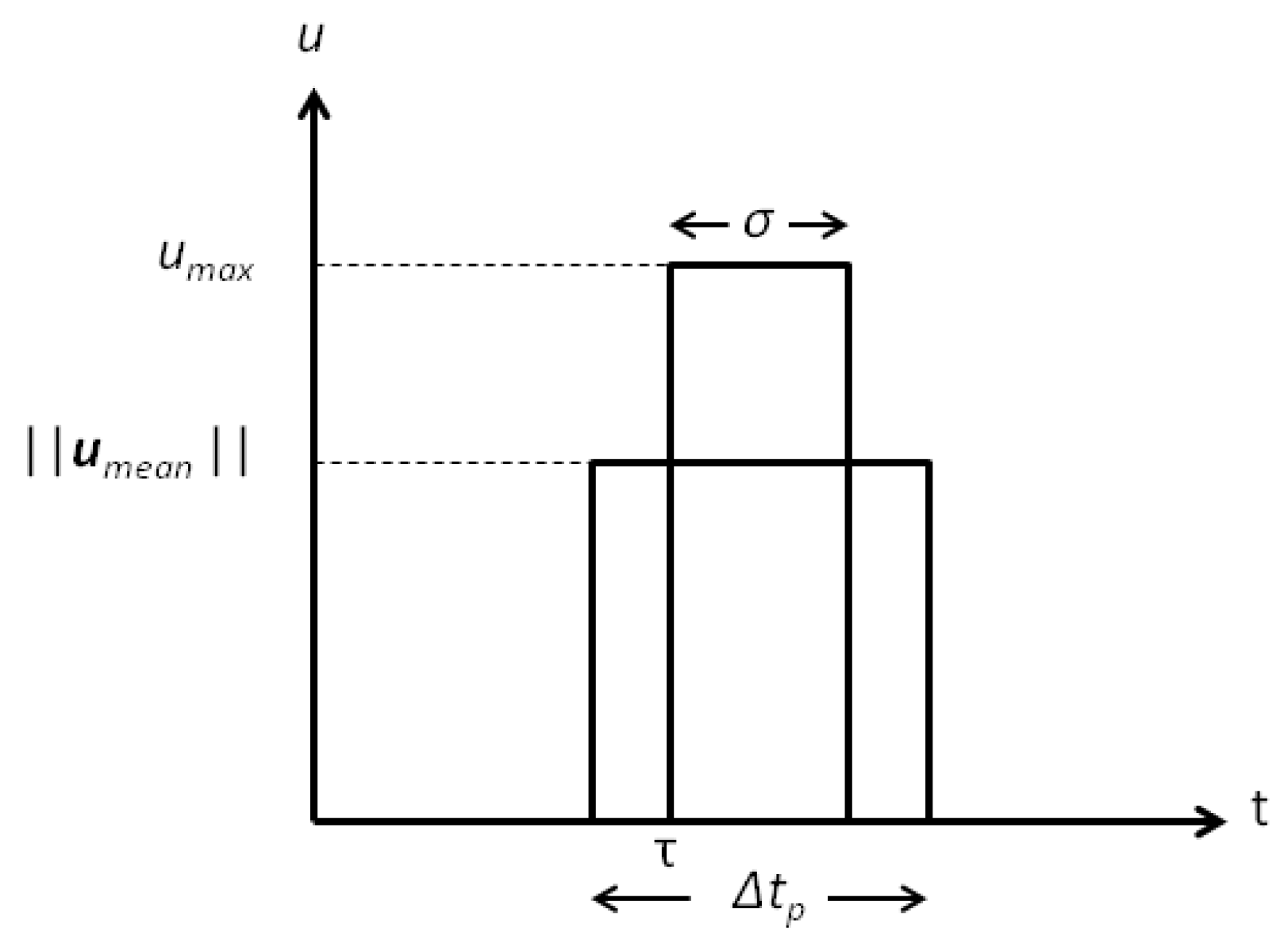
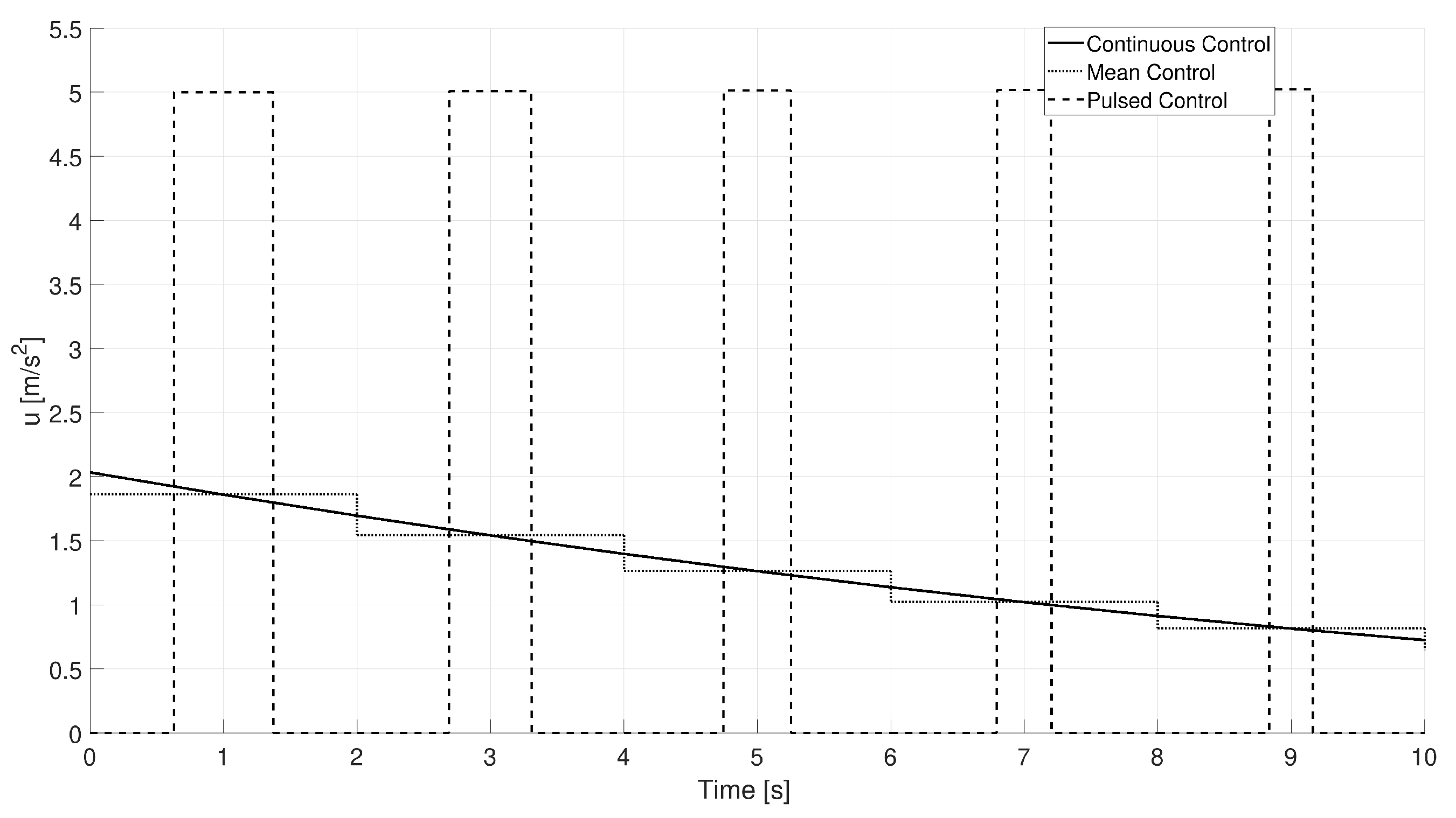
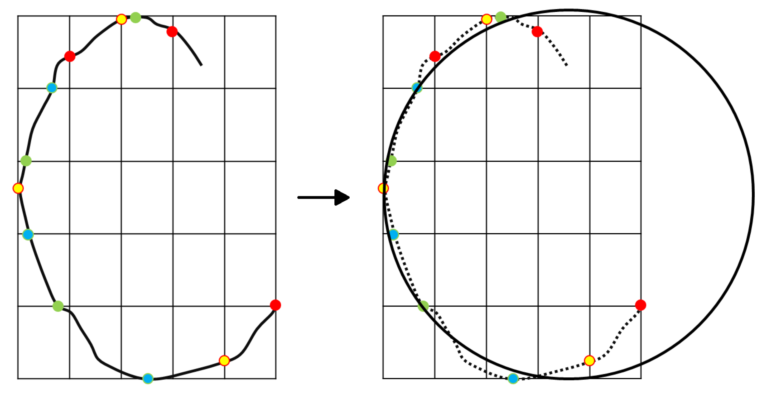
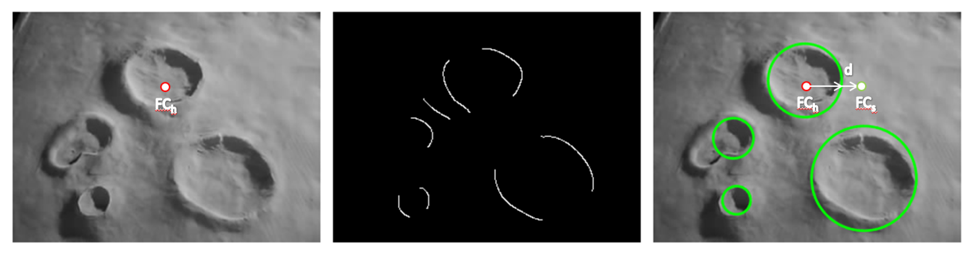
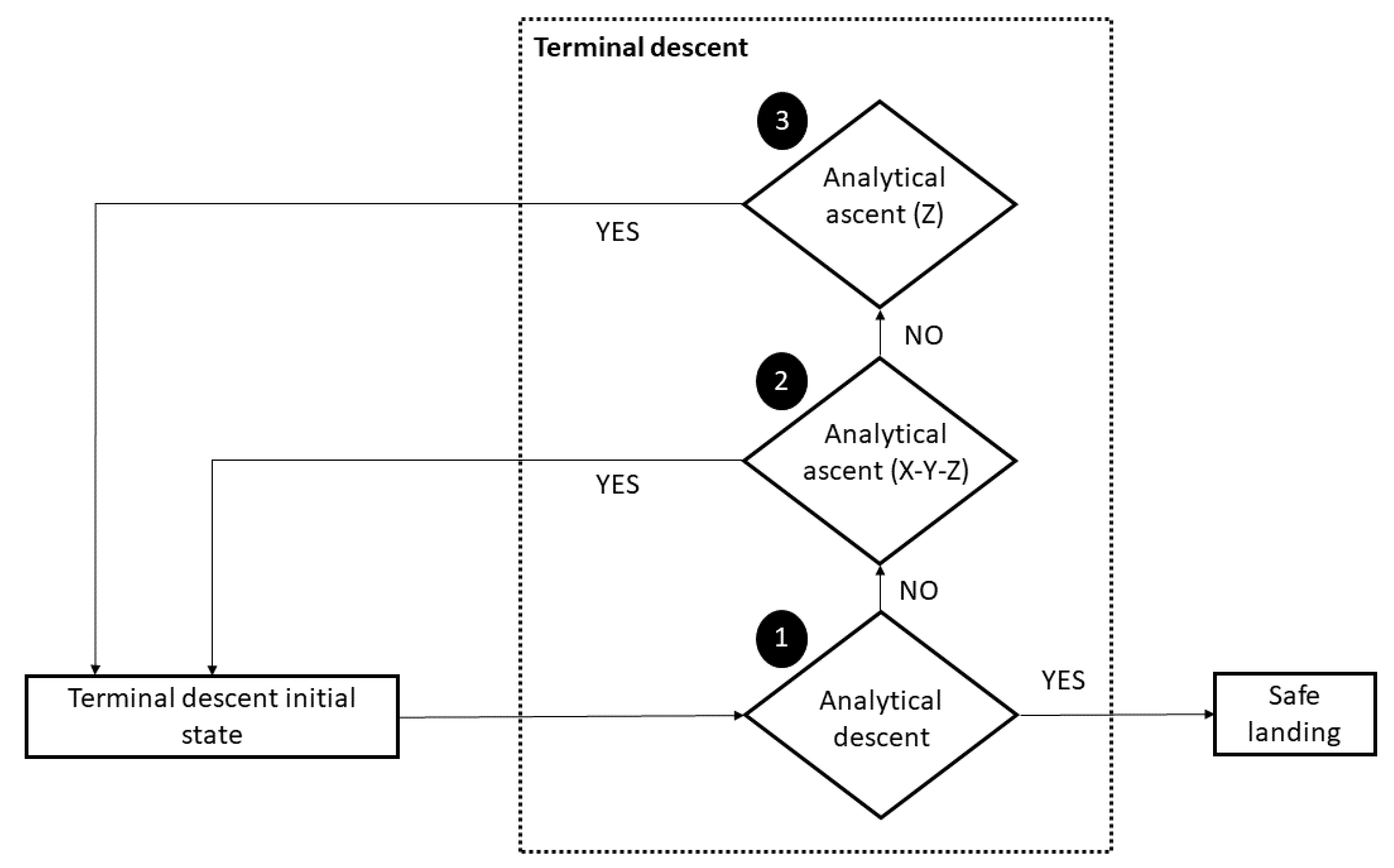
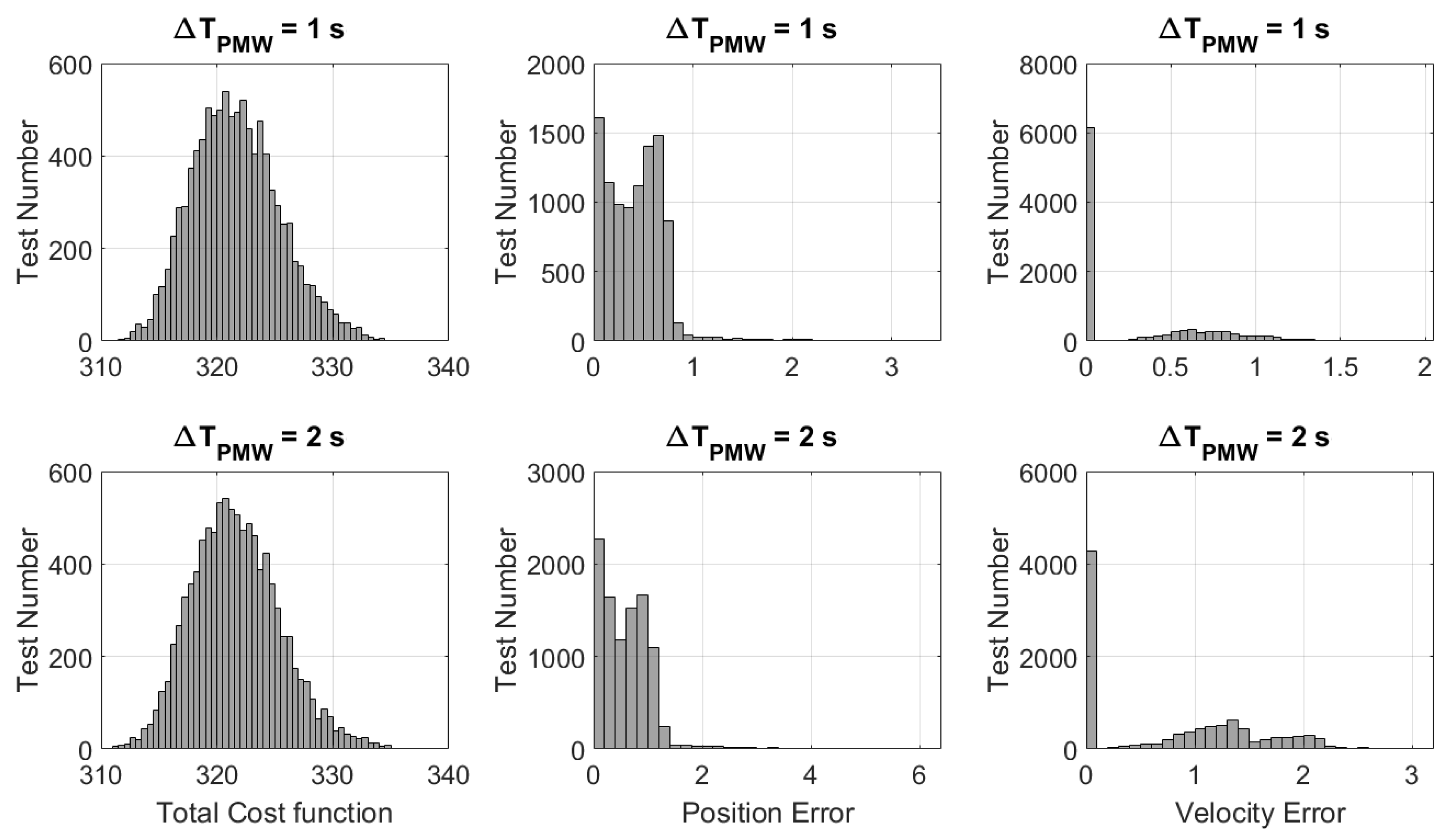
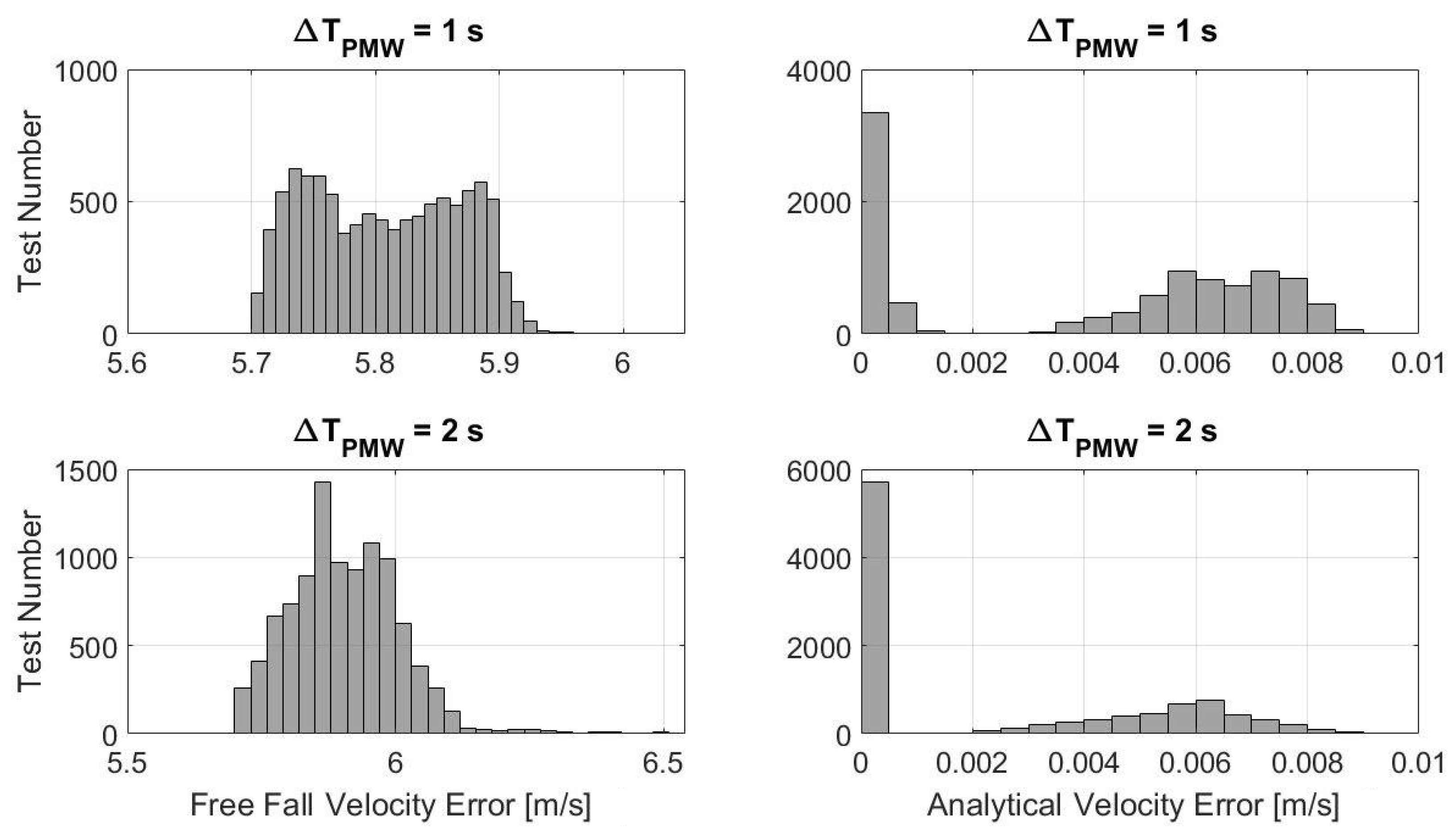
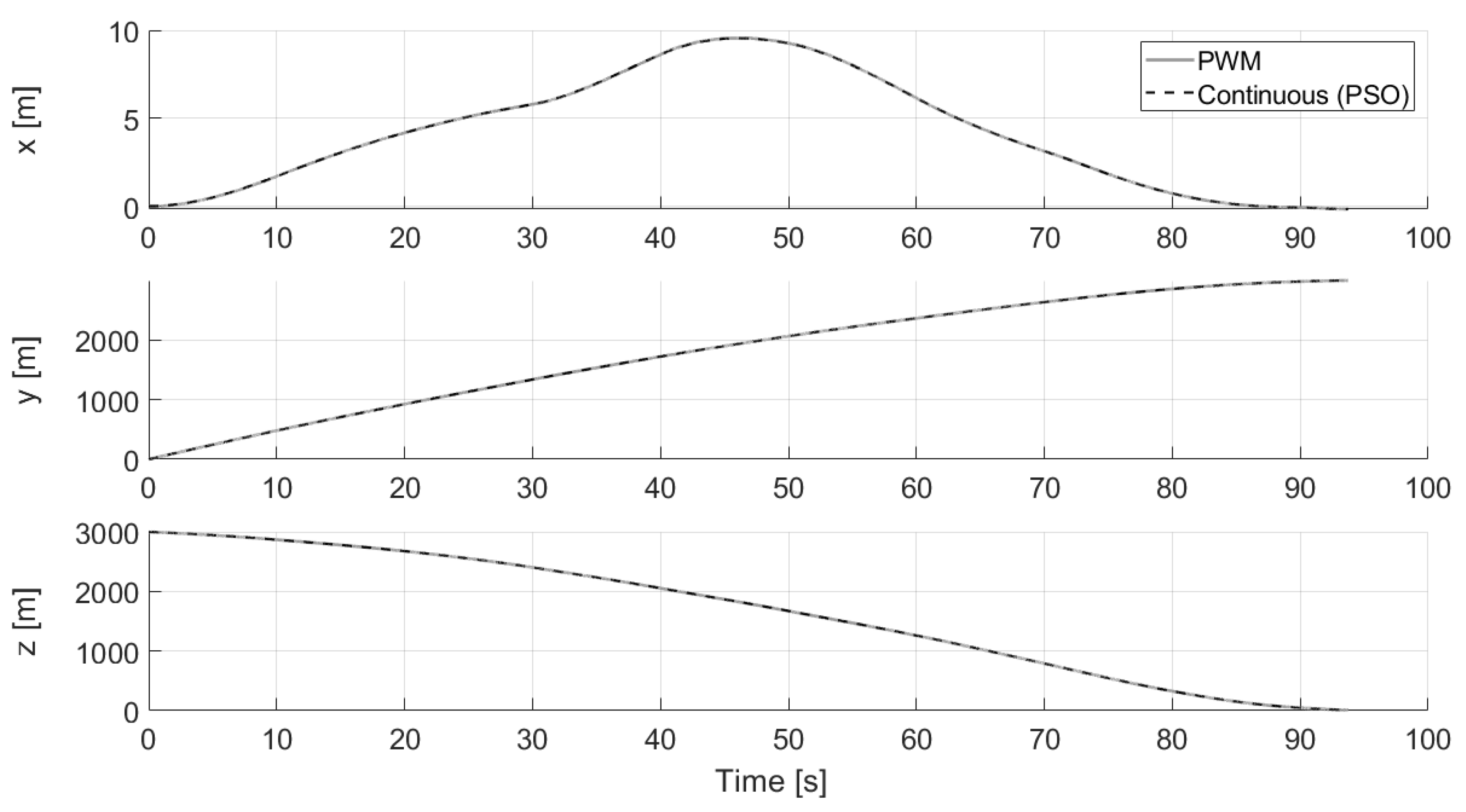
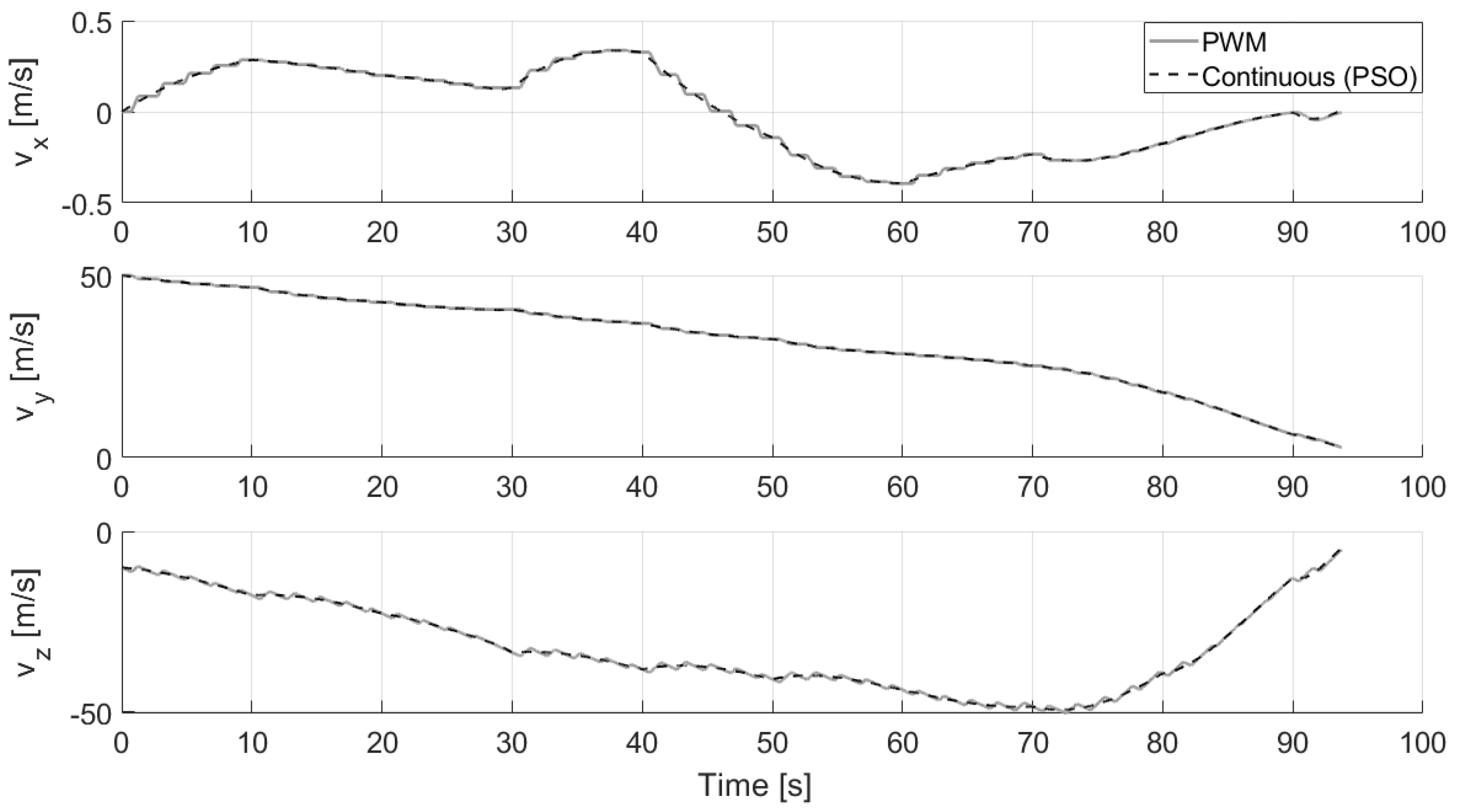
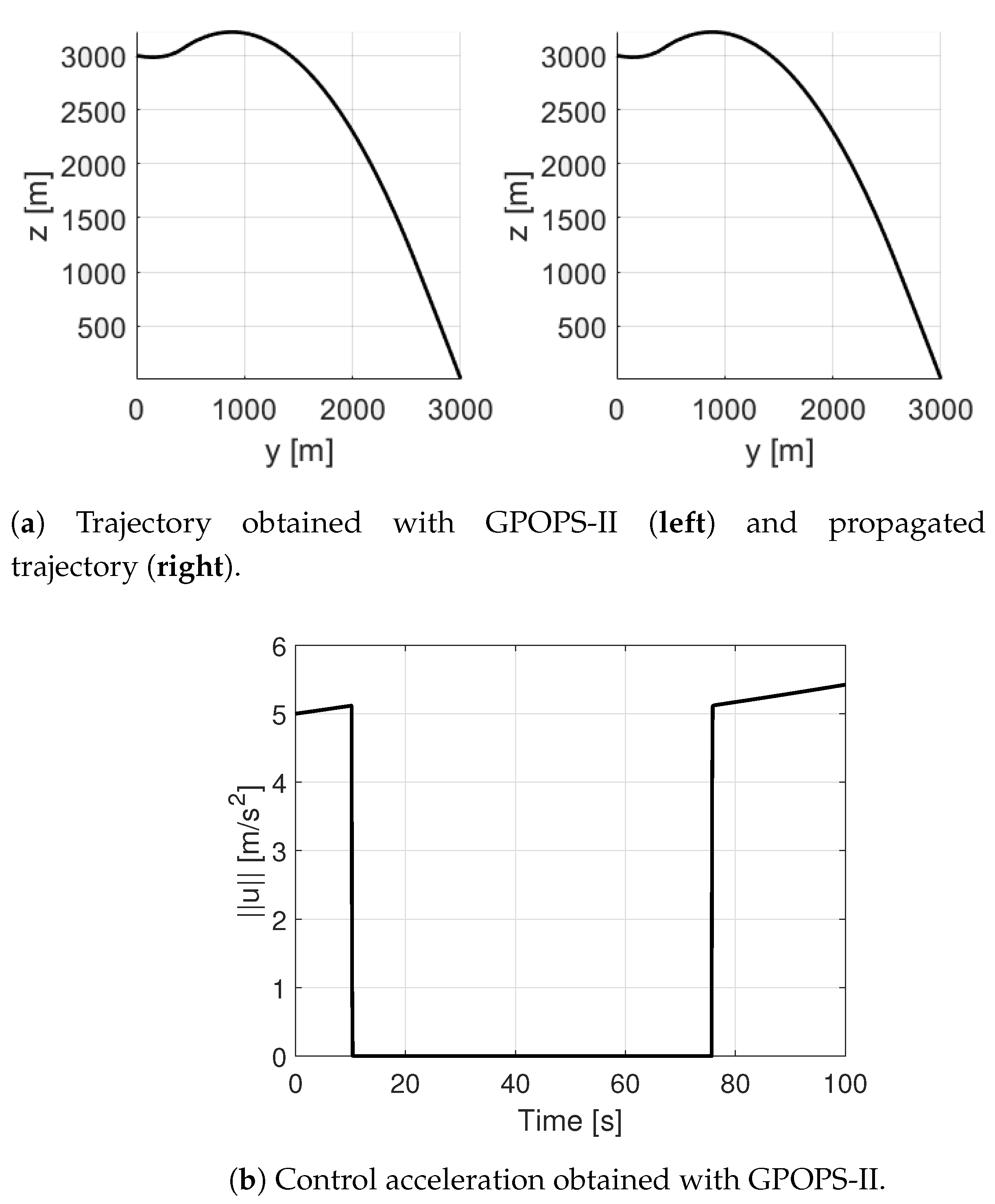
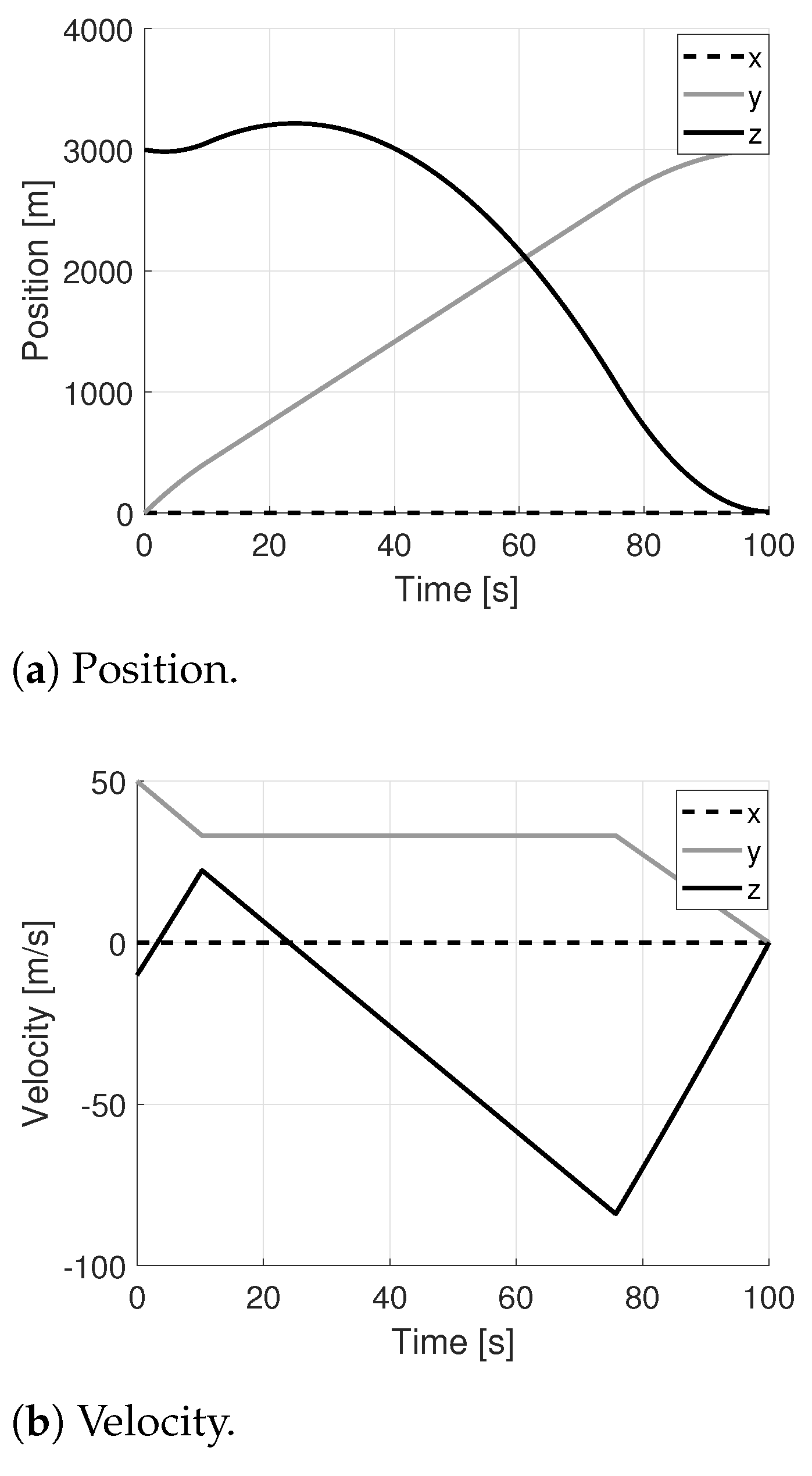
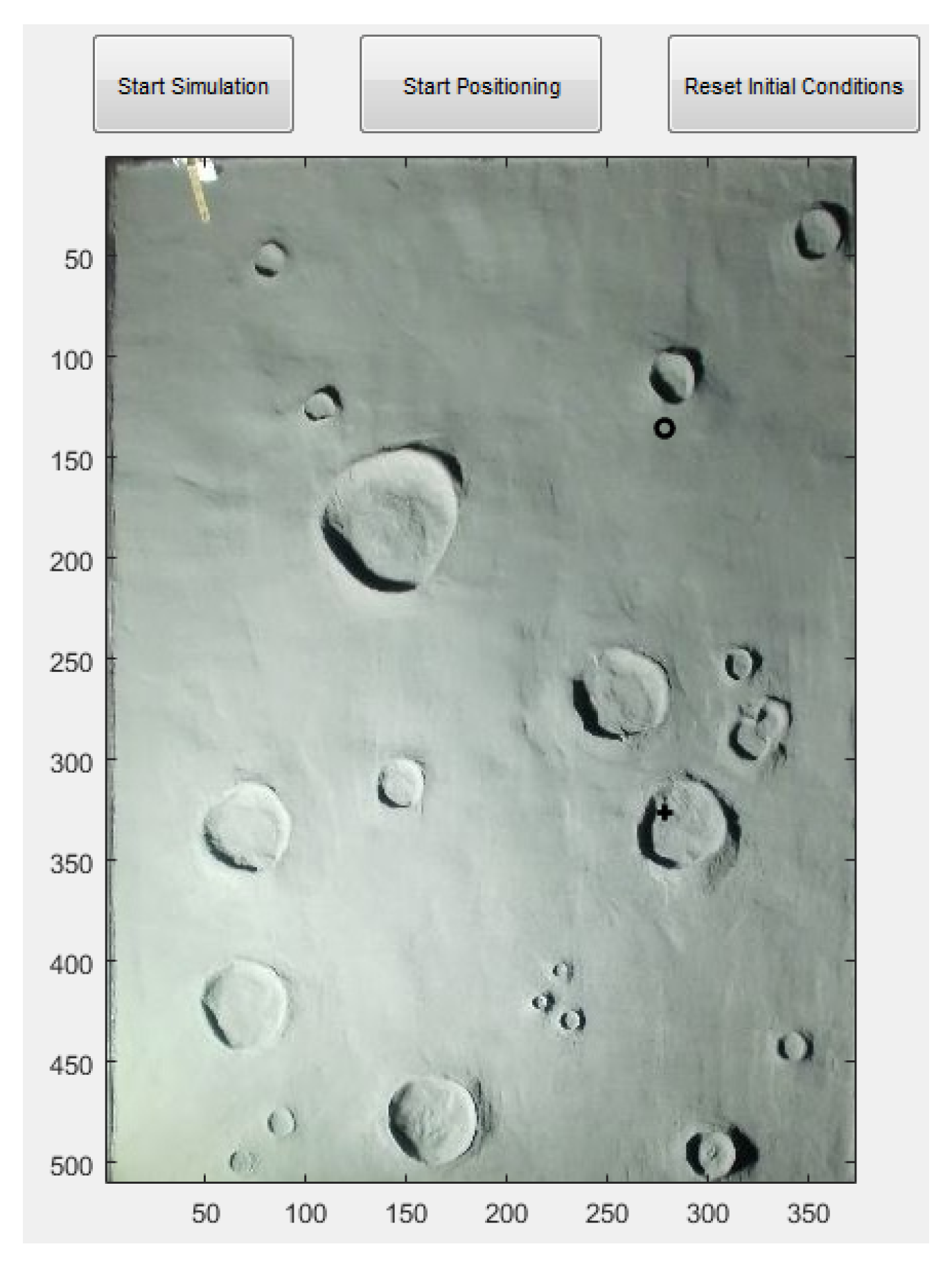
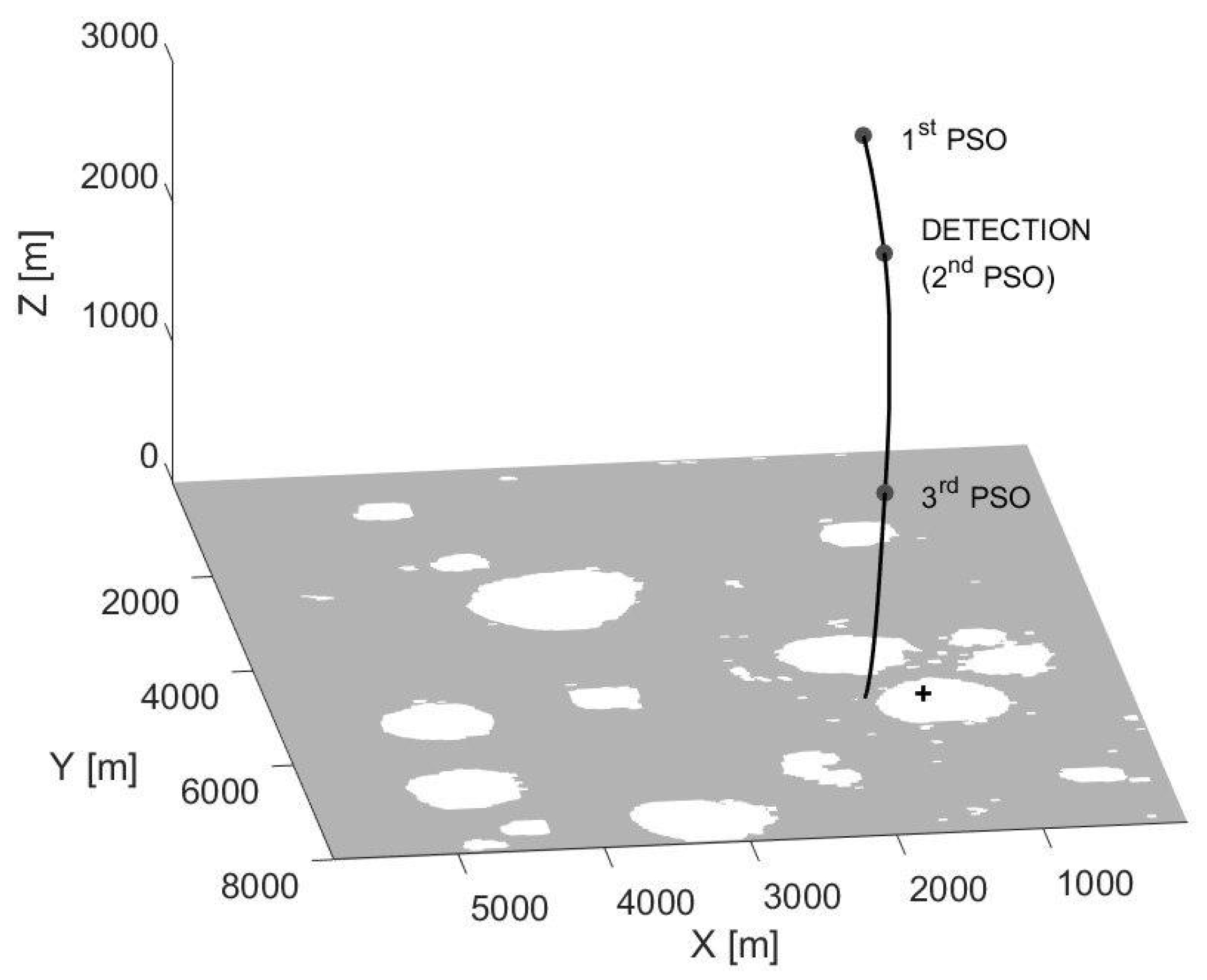
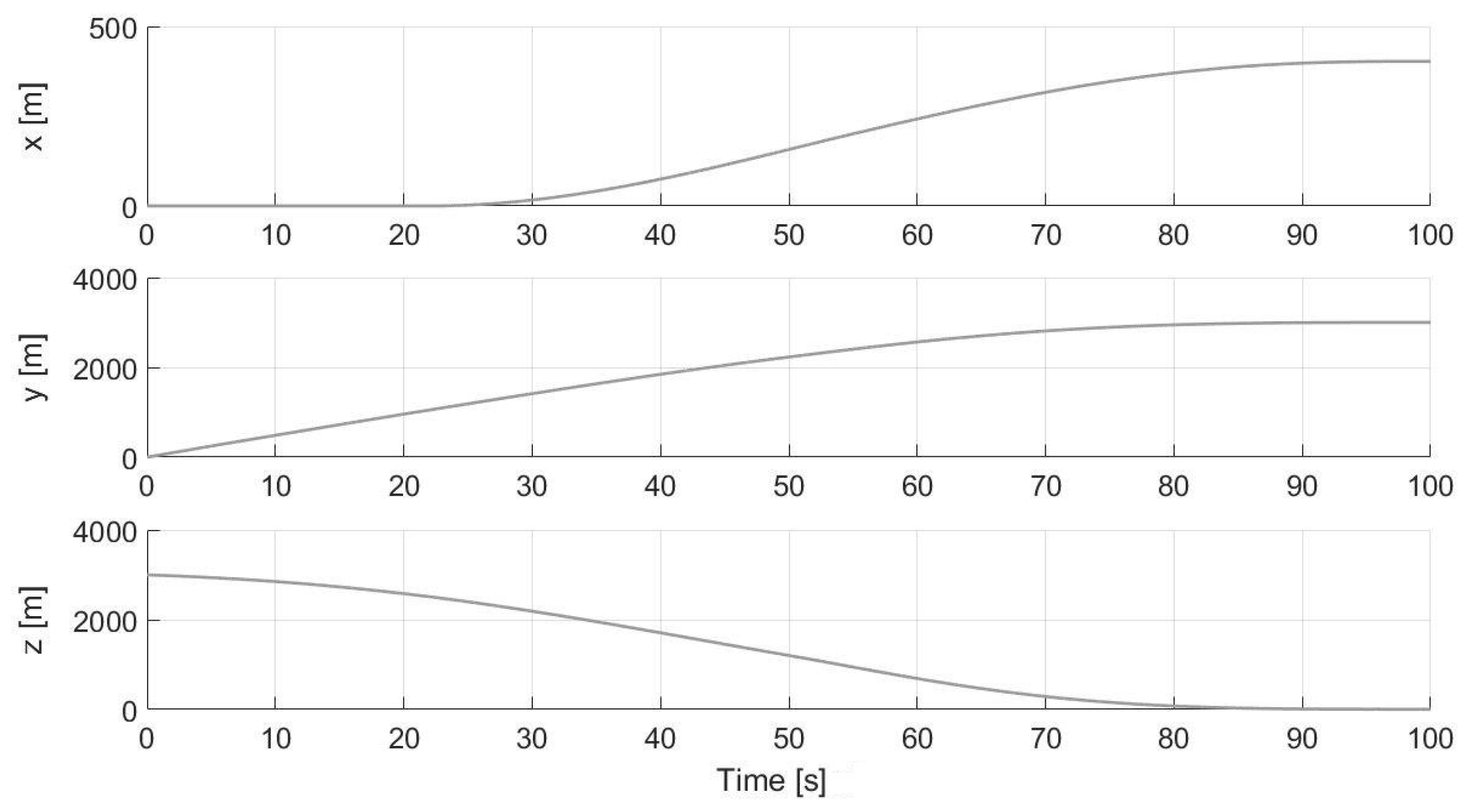
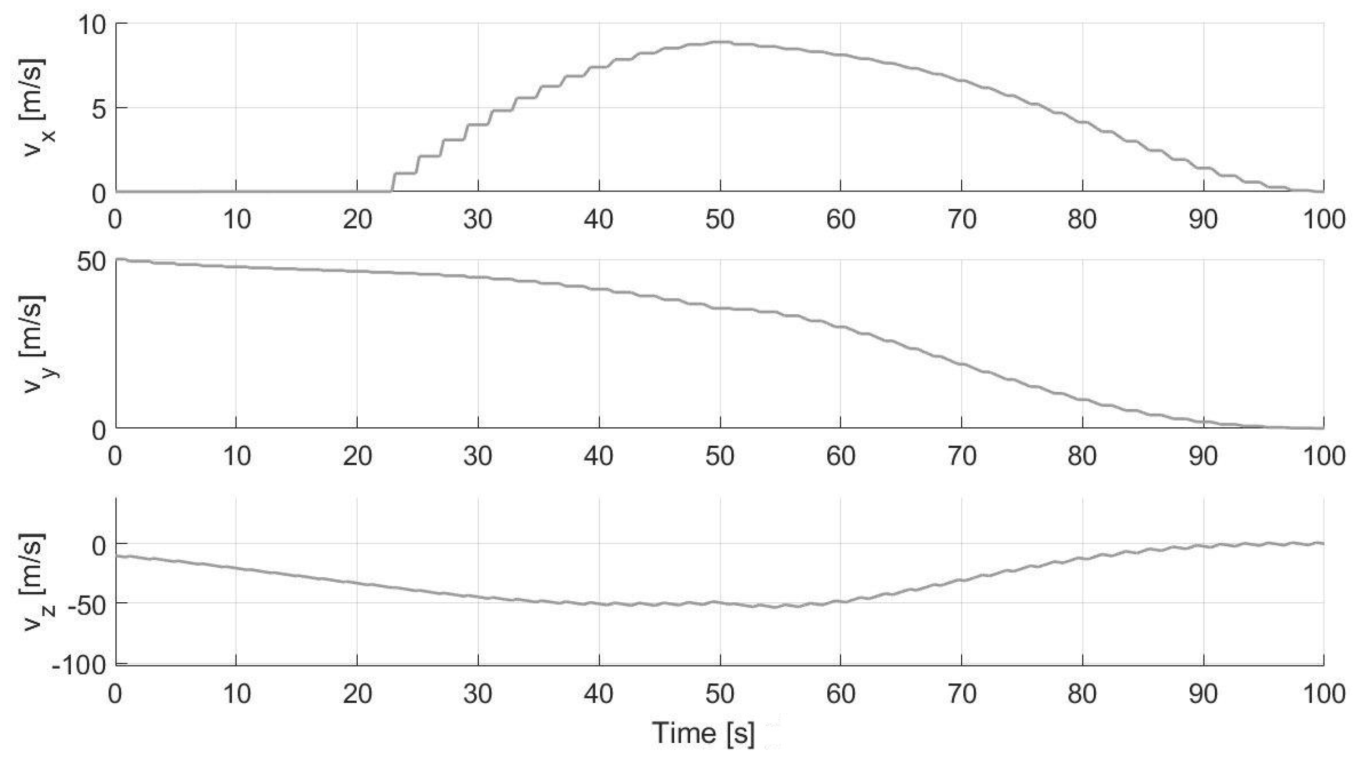
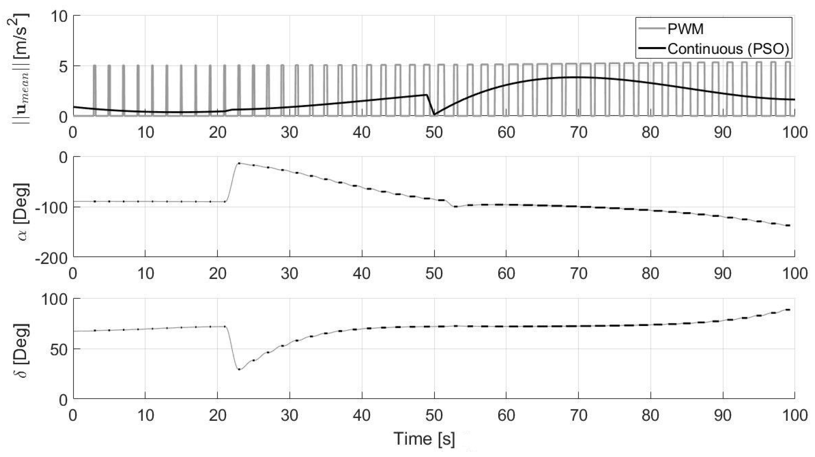
Table 1.
Summary of the performances of Monte Carlo simulations (only the feasible solutions are considered).
Table 1.
Summary of the performances of Monte Carlo simulations (only the feasible solutions are considered).
| Monte Carlo | Mean | std | min | max |
|---|---|---|---|---|
| 1 | 321.6794 | 3.7921 | 310.7846 | 337.2861 |
| 2 | 321.6643 | 3.8038 | 310.2898 | 338.6446 |
Publisher’s Note: MDPI stays neutral with regard to jurisdictional claims in published maps and institutional affiliations. |
© 2021 by the authors. Licensee MDPI, Basel, Switzerland. This article is an open access article distributed under the terms and conditions of the Creative Commons Attribution (CC BY) license (https://creativecommons.org/licenses/by/4.0/).
Share and Cite
MDPI and ACS Style
D’Ambrosio, A.; Carbone, A.; Spiller, D.; Curti, F. PSO-Based Soft Lunar Landing with Hazard Avoidance: Analysis and Experimentation. Aerospace 2021, 8, 195. https://0-doi-org.brum.beds.ac.uk/10.3390/aerospace8070195
AMA Style
D’Ambrosio A, Carbone A, Spiller D, Curti F. PSO-Based Soft Lunar Landing with Hazard Avoidance: Analysis and Experimentation. Aerospace. 2021; 8(7):195. https://0-doi-org.brum.beds.ac.uk/10.3390/aerospace8070195
Chicago/Turabian StyleD’Ambrosio, Andrea, Andrea Carbone, Dario Spiller, and Fabio Curti. 2021. "PSO-Based Soft Lunar Landing with Hazard Avoidance: Analysis and Experimentation" Aerospace 8, no. 7: 195. https://0-doi-org.brum.beds.ac.uk/10.3390/aerospace8070195
Note that from the first issue of 2016, this journal uses article numbers instead of page numbers. See further details here.