Tracking Model Predictive Control for Docking Maneuvers of a CubeSat with a Big Spacecraft

Abstract

The release and retrieval of a CubeSat from a big spacecraft is useful for the external inspection and monitoring of the big spacecraft. However, docking maneuvers during the retrieval are challenging since safety constraints and high performance must be achieved, considering the small dimensions and the actual small satellites technology. The trajectory control is crucial to have a soft, accurate, quick, and propellant saving docking. The present paper deals with the design of a tracking model predictive controller (TMPC) tuned to achieve the stringent docking requirements for the retrieval of a CubeSat within the cargo bay of a large cooperative vehicle. The performance of the TMPC is verified using a complex model that includes non-linearities, uncertainties of the CubeSat parameters, and environmental disturbances. Moreover, 300 Monte Carlo runs demonstrate the robustness of the TMPC solution.

1. Introduction

CubeSats and nanosatellites missions have gained the attention of the main actors in the space field [1]. In the last decade, the number of CubeSat missions deeply increased thanks to the low cost and fast delivery of these spacecrafts and the miniaturization of technologies that enable operations capabilities, such as orbit maneuvers both in Earth orbit and in interplanetary transfers, the absolute and relative navigation, and proximity operations.

One of the most interesting and challenging types of missions is the inspection and monitoring of orbiting spacecraft/targets, such as the International Space Station [2], the Lunar Gateway [3], as well as operative [4] and not operative [5] big satellites. These missions for inspection require a set of maneuvers for rendezvous, proximity operations and, in case, docking with the Target, as shown in [6].

Severe safety constraints and high-performance requirements are the main drivers of a retrieval phase. The spacecraft shall avoid any possible collision with the Target, i.e., (1) maintaining its trajectory out of a safety ellipse during the inspection phase [6], (2) guaranteeing passive safe trajectories in case of misbehaviors or off-nominal conditions, and (3) moving away from the Target in case of risk of collision with quick maneuvers.

The small satellites technologies are observing a strong improvement, but the required technologies needed for retrieval missions are gaining, only in the last years, the sufficient level of maturity. An in-orbit demonstration has been conducted in September 2019 by the 3U CubeSat named Seeker. It operated around Cygnus, taking images of the vehicle, and performing a set of maneuvers (such as target tracking and station-keeping) [7]. Other in orbit demo missions are planned and advanced studies are conducted to improve the level of readiness for small satellite technology: NASA, ESA, and other companies are also working on CubeSat missions for demonstrating capabilities related to formation flight and proximity operations, which have relevance for the purpose of inspecting vehicles in orbit (e.g., NanoAce 3U CubeSat flown in 2017 [8], GOM-x-4B 6U CubeSat flown in 2018 [9], CubeSat proximity operations demonstrator (CPOD) to be launched in 2021 [10].

The major technological challenges for docking are the relative navigation between the Chaser and Target based on radiofrequency sensors or vision-based information fused on advanced algorithms for the determination [11,12] the equipment to favor the identification of the docking port [13], the mating mechanisms [14], and the control system (especially for maneuvers very close to the Target), made through advanced controller and precise propulsion systems and actuators that guarantee the right level of accuracy. In particular, the last meters before the mating are crucial since the margin of error is reduced, and that is worsened by the reduced dimension of the spacecraft (and the docking mechanism), and the small satellite technology that does not provide the same performance of the one used for bigger satellites.

One way to improve the confidence level in the success of the docking phase is to adopt an effective strategy to control the relative distance between the Target and Chaser. In this sense, the problem related to the docking maneuvers is deeply investigated in literature for big satellites [15,16,17], and the docking of spacecraft with the ISS is almost a “routine” operation both for cargo and manned vehicles [18,19,20]. From the analysis of the solutions for a big spacecraft, it is possible to identify how the robustness of the control and the maneuver authority together with the execution time and, in case, the control effort are fundamental aspects that the controller must satisfy.

The range of controller for docking of a big spacecraft is large and includes optimal, robust, and adaptive control laws. In [21], the authors study controllers based on linear quadratic regulator (LQR) and proportional derivative (PD) control and present a comparative analysis between different guidance trajectories evaluated through time execution of the maneuver, fuel consumption, and mating accuracy but they do not provide the optimality of the results. Adaptive control laws for spacecraft rendezvous and docking under measurement uncertainty, such as aggregation of sensor calibration parameters, systematic bias or some stochastic disturbances, are proposed in [22]. In [23], authors show an optimized state dependent MPC that integrates a pulse width pulse frequency modulation model: The results highlight a good accuracy at the final state minimizing the control efforts and approaching time. Authors in [24] propose a guidance scheme for autonomous docking where the trajectory components of the controlled spacecraft are imposed using polynomial functions determined through optimization processes. Authors in [25] give a complete overview of the maneuver and control capabilities for the capture of a non-rotating and rotating target, using a model predictive controller (MPC) but limiting the study to planar maneuvers. Another possible solution is the model predictive controller with the tuning based on the tracking reference system optimization, as demonstrated in [26] in a docking maneuver with a non-cooperative target. Authors in [27] demonstrate how the MPC controller successfully manages the docking phase in handling constraints on state vector and control vectors, while authors in [28] investigate in detail the impact of the controller bandwidth, the line of sight cone, and exhaust plume direction constraints in the docking controller with a sophisticated model predictive control.

However, the docking of small satellites is never performed in orbit now and few papers address the control problem. Authors in [29] present the determination and control strategy for the CPOD mission, but no further details are provided on the adopted techniques. Authors in [30] present an H-infinity controller taking care of the robust stability and performance through the mu-synthesis. Authors in [31] propose and validate on a test-bench a sampling-based stochastic model predictive control (SMPC) algorithm with off-line determination of the controller weights for discrete-time linear systems subject to both parametric uncertainties and additive disturbances.

The present paper deals with the design and verification through the analysis of a tracking model predictive control (TMPC). The focus is to guarantee a high accuracy on the trajectory tracking and the final point accuracy, minimizing the approach velocity, maintaining an execution time lower than 10 min, and reducing the control effort in the nominal conditions.

Section 2 presents the problem formulation. Section 3 shows the design process of MPC and tuning of the tracking model predictive controller for the docking maneuvers. Section 4 describes the simulation architecture and setup, the results of the simulation in terms of performance of the controller in the worst nominal case (Section 4.1), and the robustness analysis, made through a Monte Carlo simulation (Section 4.2). Section 5 concludes the paper with final remarks and the future perspectives of the work.

2. Problem Formulation

The objective is the control of the relative position between the docking mechanism and the docking port. The problem formulation is based on the definition of the adopted reference frames and assumptions on the motion conditions and the spacecraft features.

2.1. Reference Frames

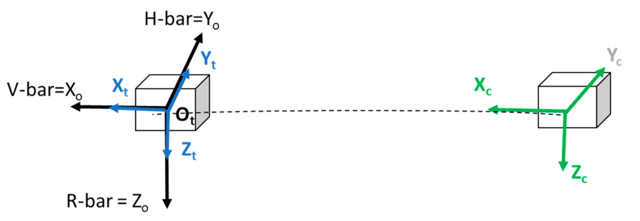
Three reference frames are defined in order to formulate the problem (Figure 1).

• The spacecraft local orbital frame (R_o) has its origin O_o in the center of mass (CoM) of the spacecraft; X_o is defined such that X_o = Y_o × Z_o (X_o is in the direction of the orbital velocity vector but not necessarily aligned with it), Y_o is in the opposite direction of the angular momentum vector of the orbit, and Z_o is radial from the spacecraft CoM to the center of the Earth. As reported in literature, in this paper, the X-axis is called V-bar, Y-axis is called H-bar, and Z-axis is called R-bar.
• The Target body frame (R_t) has origin O_t in the Target CoM, the directions of the axes are along the main inertia axes of the Target and Z_t = X_t × Y_t forming a right-handed system.
• The Chaser body frame (R_c) has origin O_c in the Chaser CoM, the directions of the axes are along the main inertia axes of the Chaser and Z_c = X_c × Y_c forming a right-handed system.

2.2. Assumptions

The problem formation is based on a set of assumptions on the initial and motion conditions:

• Assumption 1 (Last Hold Point orbit conditions): The control starts in the final hold point (HP) at 50 m of distance between the Chaser and Target. In addition, the Chaser is already aligned with the Target. This assumption allows considering guidance strategies based on straight-line approaches without relevant fly-around maneuvers. It could be considered compliant with a real mission in which a GO/No Go command is expected from the ground before the beginning of the final and very delicate docking maneuvers and after a check of the nominal operativity of the Chaser (and the Target) [6]. The achievement of this final hold point depends on the previous mission phases that could introduce an uncertainty on the real position and velocity of the CubeSat in HP.
• Assumption 2 (Chaser and Target mass): The Chaser is a 12U CubeSat (20 × 20 × 30 cm) whose mass (m_c) is 20 Kg and the Target is a vehicle whose mass (m_t) is 2000 Kg.
• Assumption 3 (Location of the docking port and docking mechanism): Due to the small dimensions of the satellites and considering a fixed distance of the docking port with respect to O_c along Z_c axis and the fixed distance of the docking mechanism with respect to O_t along Z_t axis, it is assumed that the docking port and the docking mechanism are in coincidence of O_t and O_c, respectively.

Finally, the big Target is considered cooperative and its motion is controlled, as in [32].

3. Control Design

The goal of the controller is to reach the soft docking performance in

Table 1. Final requirements.

Requirement	Required Performance
Approach velocity [m/s]	<0.02
Lateral alignment [m]	<0.01
Lateral velocity [m/s]	<0.01

under safety constraints. The controller shall control the relative position and velocity between the Chaser and Target, according to the strategies defined for any phase. The controlled state variables are: The relative position (X, Y, Z) and velocity (V_x, V_y, V_z) between the Chaser CoM (O_ch) and the Target CoM (O_tg).

A tracking model prediction controller (TMPC) is designed for the control of the trajectory. The advantages of this technique for the docking problem are: (1) The possibility to constrain the input, the state and output imposing boundaries whose violation is prevented and (2) the capability to define the guidance strategy and, even, the capability to follow the reference trajectory. Constraints on fuel consumption, time to capture, and safety conditions of the maneuver can be introduced. TMPC drives the state variables to their optimal set points (i.e., the relative position and attitude can be optimized to meet the soft docking requirements), while others can be held within the defined boundaries (i.e., the velocity can be regulated with specific profiles). The prediction of the future states leads to the definition of the optimal trajectory. TMPC aims at solving the reference tracking optimization problem, posing great importance on the capability of the controller to track the desired values.

3.1. Trajectory Control

The model predictive control is based on the optimization criterion defined as:

$$J\left(U\left(k\right),x\left(k|k\right)\right)={\displaystyle \sum }_{i=0}^{H_p-1}L\left(x\left(k+i|k\right),U\left(k+i|k\right)\right)+{\mathsf{\Phi }}_{\mathrm{W}}\left(x\left(k+H_p|k\right)\right)$$

(1)

where $H_p$ is the prediction horizon, $L\left(.\right)$ is the weight function, ${\mathsf{\Phi }}_{\mathrm{W}}\left(x\left(k|k\right)\right)$ is the terminal state weight function, $x\left(k|k\right)$ is the state measurement at time k, and U(k+1|k) is the control action at time k+1 given k. In particular, the weighting functions are characterized by:

$$\left(x,u\right)=x^{T}Qx+u^{T}Ru$$

(2)

$${\mathsf{\Phi }}_{\mathrm{W}}\left(x\left(k|k\right)\right)=x^{T}Px$$

(3)

where Q, R, and P matrices are symmetric positive definite matrices.

Substituting (2) and (3) in (1), the optimization criterion can be written as:

$$J\left(U\left(k\right),x\left(k|k\right)\right)={\displaystyle \sum }_{i=0}^{H_p-1}x{\left(k+i|k\right)}^{T}Qx\left(k+i|k\right)+u{(k+i|k)}^{T}Ru(k+i|k)+x{\left(k+H_p|k\right)}^{T}Px\left(k+H_p|k\right)$$

(4)

In order to set the optimization problem in a quadratic formulation, (4) can be rewritten as:

$$J\left(U\left(k\right),x\left(k|k\right)\right)=\frac{1}{2}X{\left(k\right)}^T\mathcal{Q}X\left(k\right)+U\left(k\right)\mathcal{R}U\left(k\right)$$

(5)

where:

$$X\left(k\right)=\left[\begin{array}{cccc}x\left(k|k\right)& x\left(k+2|k\right)& \dots & x\left(k+H_p|k\right)\end{array}\right]$$

$$U\left(k\right)=\left[\begin{array}{cccc}u\left(k|k\right)& u\left(k+1|k\right)& \dots & u\left(k+H_p-1|k\right)\end{array}\right]$$

$$\mathcal{R}=\left[\begin{array}{ccc}R& \dots & 0\\ \dots & \dots & \dots \\ 0& \dots & R\end{array}\right] \mathcal{Q}=\left[\begin{array}{ccc}Q& \dots & 0\\ \dots & Q& \dots \\ 0& \dots & P\end{array}\right]$$

The MPC control requires the prediction of the future states until the prediction horizon $H_p$ through the augmented system is described by:

$$X\left(k\right)=\mathcal{A}x\left(k|k\right)+\mathcal{B}U\left(k\right)$$

(6)

where:

$$\mathcal{A}={\left[\begin{array}{cccc}A& A^2& \dots & A^{H_p}\end{array}\right]}^T \mathcal{B}=\left[\begin{array}{ccccc}B& 0& \dots & 0& 0\\ AB& B& \dots & 0& 0\\ \dots & \dots & \dots & \dots & \dots \\ A^{H_p-2}B& A^{H_p-1}B& \dots & B& 0\\ A^{H_p-1}B& A^{H_p-2}B& \dots & A^{2}B& AB\end{array}\right]$$

The cost functions of MPC with the predictions are obtained substituting (6) in (5):

$$\begin{gathered} J\left(U\left(k\right),x\left(k|k\right)\right)=\frac{1}{2}{\left[\mathcal{A}x\left(k|k\right)+\mathcal{B}U\left(k\right)\right]}^T\mathcal{Q}\left[\mathcal{A}x\left(k|k\right)+\mathcal{B}U\left(k\right)\right]+U\left(k\right)\mathcal{R}U\left(k\right)=\left[x{\left(k|k\right)}^T{\mathcal{A}}^T\mathcal{Q}\mathcal{A}x\left(k|k\right)+ \\ U{\left(k\right)}^T\left[{\mathcal{B}}^T\mathcal{Q}\mathcal{B}+\mathcal{R}\right]U\left(k\right)+2x{\left(k|k\right)}^T{\mathcal{A}}^T\mathcal{Q}\mathcal{B}U\left(k\right)\right]=U{\left(k\right)}^T{H}_{opt}U\left(k\right)+x{\left(k|k\right)}^T{F}_{opt}U\left(k\right)+\overline{J}\left(x\left(k|k\right)\right) \end{gathered}$$

(7)

where $H_{opt}={\mathcal{B}}^T\mathcal{Q}\mathcal{B}+\mathcal{R} , F_{opt}=2{\mathcal{A}}^T\mathcal{Q}\mathcal{B}$, $\overline{J}\left(x\left(k|k\right)\right)={\mathcal{A}}^T\mathcal{Q}\mathcal{A}$.

The final formulation of the control problem is a constrained optimization problem, which must be solved at each time step:

$$\left\{\begin{array}{c}\min J\left(U\left(k\right),x\left(k|k\right)\right)=\min U{\left(k\right)}^T{H}_{opt}U\left(k\right)+x{\left(k|k\right)}^T{F}_{opt}U\left(k\right)\\ s.t.\\ x\left(k+1|k\right)=Ax\left(k|k\right)+BU\left(k\right):\\ U\left(k\right)\in \mathbb{U}\\ x\left(k+i|k\right)\in X, i=1,2,\dots ,H_p\\ x\left(k+H_p|k\right)\in {\mathbb{X}}_F\subset \mathbb{X}\end{array}\right.$$

(8)

where $\mathbb{U}$,$\mathbb{X},$ and ${\mathbb{X}}_F$ are, respectively, the input constraint set, the state constraint set, and the terminal constraint set.

Considering a quadratic criterion and a linear constraint set, the optimization problem becomes a quadratic programming problem. The control is applied via the receding horizon principle, based on three following steps at each time: (1) To get the state $x\left(k\right)$, (2) to solve the optimization problem to find the predicted unforced response $U^o\left(k\right)=\left[\begin{array}{cccc}{u}^o(k|k)& u^o(k+1|k)& \dots & u^o(k+H_p|k)\end{array}\right]$, and (3) to apply the control action $u\left(k\right)=u^o\left(k,k\right)$.

3.2. Tracking Model Predictive Control

For the trajectory control, the tracking model prediction control is adopted, that optimizes the reference tracking. The optimization criterion (5) is modified by introducing the reference vector r(k) for the prediction:

$$J\left(U\left(k\right),x\left(k|k\right)\right)={\displaystyle \sum }_{i=0}^{H_p-1}{\left(x\left(k+i|k\right)-r\left(k+i\right)\right)}^{T}Q\left(x{\left(k+i|k\right)}^T-r\left(k+i\right)\right)+u{(k+i|k)}^{T}Ru(k+i|k)$$

(9)

Considering the augmented system (6) and introducing the augmented reference vector $R\left(k\right)=\left[\begin{array}{cccc}r\left(k\right)& r\left(k+1\right)& \dots & r\left(k+H_p\right)\end{array}\right]$, (8) can be written as:

$$\begin{gathered} J\left(U\left(k\right),x\left(k|k\right)\right)={\left[\mathcal{A}x\left(k|k\right)+\mathcal{B}U\left(k\right)-R\left(k\right)\right]}^T\mathcal{Q}\left[\mathcal{A}x\left(k|k\right)+\mathcal{B}U\left(k\right)-R\left(k\right)\right]+U\left(k\right)\mathcal{R}U\left(k\right) \\ =\left[x{\left(k|k\right)}^T{\mathcal{A}}^T\mathcal{Q}\mathcal{A}x\left(k|k\right)+U{\left(k\right)}^T\left[{\mathcal{B}}^T\mathcal{Q}\mathcal{B}+\mathcal{R}\right]U\left(k\right)+2x{\left(k|k\right)}^T{\mathcal{A}}^T\mathcal{Q}\mathcal{B}U\left(k\right) \\ -2R{\left(k\right)}^T\mathcal{Q}\mathcal{A}x\left(k|k\right)+2R{\left(k\right)}^T\mathcal{Q}\mathcal{B}U\left(k\right)+R{\left(k\right)}^T\mathcal{Q}R\left(k\right)\right] \end{gathered}$$

(10)

Substituting $H_{opt}={\mathcal{B}}^T\mathcal{Q}\mathcal{B}+\mathcal{R} ; F_{opt}=2\left[\begin{array}{c}\begin{array}{c}{\mathcal{A}}^T\mathcal{Q}\mathcal{B}\end{array}\\ QB\end{array}\right]$, the optimization criterion (10) becomes a quadratic formulation described by the cost function in (11):

$$J\left(U\left(k\right),x\left(k|k\right)\right)=U{\left(k\right)}^T{H}_{opt}U\left(k\right)+{\left[\begin{array}{c}x\left(k|k\right)\\ R\left(k\right)\end{array}\right]}^T{F}_{opt}U\left(k\right)+\overline{J}\left(x\left(k|k\right),R\left(k\right)\right)$$

(11)

and the final formulation of the problem is (12):

$$\left\{\begin{array}{c}\min \left\{U{\left(k\right)}^{T}HU\left(k\right)+{\left[\begin{array}{c}x\left(k|k\right)\\ R\left(k\right)\end{array}\right]}^{T}FU\left(k\right)+\overline{J}\left(x\left(k|k\right),R\left(k\right)\right)\right\}\\ s.t.\\ x\left(k+1|k\right)=Ax\left(k|k\right)+Bu\left(k\right)\\ U\left(k\right)\in \mathbb{U}\\ x\left(k+i|k\right)\in X, i=1,2,\dots ,H_p\\ x\left(k+H_p|k\right)\in {\mathbb{X}}_F\subset \mathbb{X}\end{array}\right.$$

(12)

where $\mathbb{U}$,$\mathbb{X},$ and ${\mathbb{X}}_F$ are, respectively, the input constraint set, the state constraint set, and the terminal constraint set.

The inputs are constrained by the maximum force of the actuators and are defined as $-u_{max}<U\left(k\right)<u_{max}$.

The state constraints are derived from the definition of the cone-shaped approach corridor. There are no state constraints on the MPC of the attitude. The terminal constraints $x\left(k+H_p|k\right)$ are fixed to 0. The adopted algorithm for the solution of minimization problem is based on “primal-dual” interior point algorithms. This algorithm has been already used on the test bench of the project CADET [33] and test on the “in the loop simulator” in [34] for the case of small satellites. In this last case, the algorithm is loaded on a micro-controller based on an ARM-9 architecture and a preliminary controller in the loop simulation performed: The execution time of the control algorithm is around 25 ms.

3.3. TMPC Design

The assumptions of small initial relative position and short maneuver time allow us to use the well-known Hill-Clohessy-Wiltshire model [35], describing the motion of a spacecraft (called the Chaser) relative to a nominal point traveling in a circular orbit (called the Target orbit). This model is described by the following Equation (13):

$${\ddot{\mathrm{x}}}_c-2\Omega {\dot{z}}_c=\frac{F_{cx}}{m_c}$$

$${\ddot{y}}_c+{\Omega }^2{y}_c=\frac{F_{cy}}{m_c}$$

(13)

$${\ddot{z}}_c+2\Omega {\dot{x}}_c-3{\Omega }^2{z}_c=\frac{F_{cz}}{m_c}$$

where $x_c$, $y$_c, $z_c$ are the relative Chaser positions, $m_c$ is its mass, 𝛺 is the angular frequency of the Target orbit, and $F_{cx}$, $F_{cy},$ and $F_{cz}$ are the external forces applied to the Chaser.

Equation (12) can be represented in the form of the state equation as follows:

$$\dot{x}=Ax+Bu$$

where $x$ = ($x_c$, $y_c$, $z_c$, ${\dot{x}}_c$, ${\dot{y}}_c, {\dot{z}}_c$) is the state vector, constituted by the three components of the Chaser position and velocity with respect to R_t, $u$ = ($F_{cx}$,$F_{cy}$,$F_{cz}$) is the force vector, and

$$A=\left[\begin{array}{cccccc}0& 0& 0& 1& 0& 0\\ 0& 0& 0& 0& 1& 0\\ 0& 0& 0& 0& 0& 1\\ 0& 0& 0& 0& 0& 2{\Omega }^{}\\ 0& -{\Omega }^2& 0& 0& 0& 0\\ 0& 0& 3{\Omega }^2& -2{\Omega }^{}& 0& 0\end{array}\right] B=\left[\begin{array}{ccc}0& 0& 0\\ 0& 0& 0\\ 0& 0& 0\\ \frac{1}{m_c}& 0& 0\\ 0& \frac{1}{m_c}& 0\\ 0& 0& \frac{1}{ m_c}\end{array}\right]$$

The TMPC control is obtained by solving, at each sampling time, the optimization problem in Equation (8), according to the receding horizon strategy described in the above section. In the optimization problem, the model function is $f\left(x,u\right)=Ax+Bu$. The input constraint set $U_c$ is defined by the following inequalities:

$$-F_{cmax}\le U_c\le F_{cmax}$$

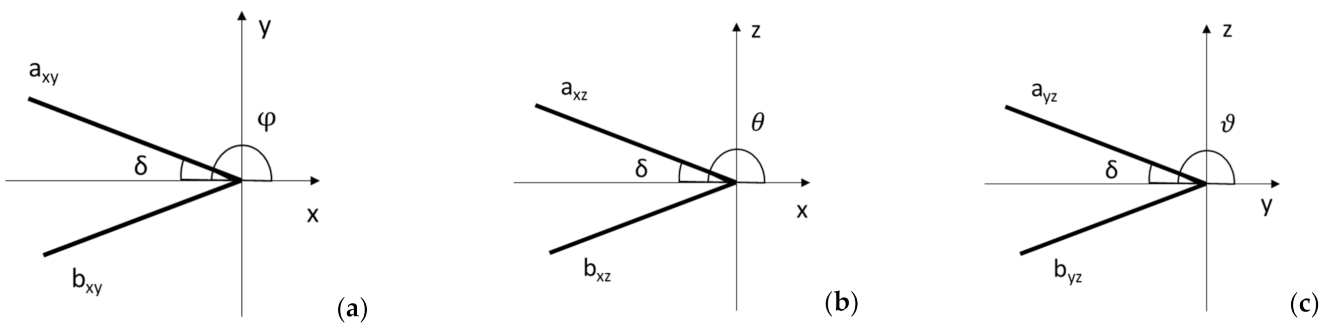
where $F_{cmax}$ is the vector of the maximum thruster forces and the inequalities are element-wise. The state constraints depend on the approach corridor represented by the cone that originated from the mating point and with a half cone angle of $\delta$. Considering the assumptions made in Section 2, the cone is univocally defined for the straight-line maneuver, and is generated from the final, docking point. In addition, it is centered in the docking axis, the X_c axis. Therefore, the state constraint set is defined by the following inequalities:

$$a_{xy}=-x_c\sin \left(\phi -\delta \right)+y_c\cos \left(\phi -\delta \right)\ge 1$$

(14a)

$$b_{xy}=x_c\sin \left(\phi +\delta \right)-y_c\cos \left(\phi +\delta \right)\ge 1$$

(14b)

$$a_{xz}=-z_c\sin \left(\theta -\delta \right)+x_c\cos \left(\theta -\delta \right)\ge 1$$

(14c)

$$b_{xz}=z_c\sin \left(\theta +\delta \right)-x_c\cos \left(\theta +\delta \right)\ge 1$$

(14d)

$$a_{yz}=-y_c\sin \left(\vartheta -\delta \right)+z_c\cos \left(\vartheta -\delta \right)\ge 1$$

(14e)

$$b_{yz}=y_c\sin \left(\vartheta +\delta \right)-z_c\cos \left(\vartheta +\delta \right)\ge 1$$

(14f)

where $a_{xy}$, $a_{xz}$, $b_{xy}$, and $b_{xz}$ represent the corridor limits, and $\phi$ and $\theta$ are the angles between the docking axis and R_t axes, as shown in Figure 2. These angles are assumed constant for the entire prediction horizon [26] and for the entire maneuver duration.

TMPC weight matrices Q and R (defined as Q = diag (Q₁₁, Q₂₂, Q₃₃, Q₄₄, Q₅₅, Q₆₆), R = diag (R₁₁, R₂₂, R₃₃)) are tuned to satisfy the requirements in Table 1. The best tuned parameters can be obtained through an iterative model and simulation-based approach, varying Q and R weights and assessing the accuracy in the mating point achievement, the quickness of trajectory acquisition and tracking performance, the control effort, and the duration of the maneuver.

4. Simulation with a Non-Linear Model with Uncertainties

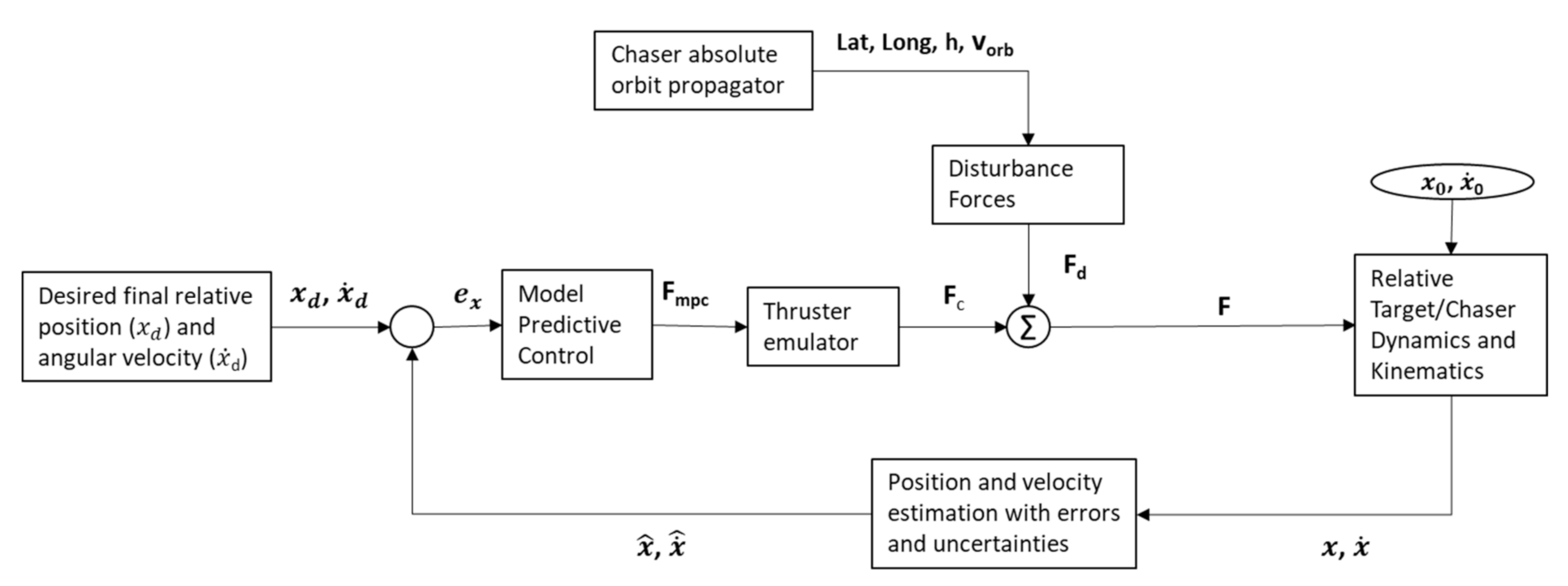
The controller performance is verified using a detailed model and a robust simulation architecture built in the Simulink © environment (Figure 3). This architecture includes the control forces (F_c) added to the disturbance forces due to the drag [36] and J2 [37] perturbations. In particular, the drag force is modelled by:

$$F_{drag}=\frac{1}{2}{C}_{D}A\rho V^2$$

(15)

where C_D = 2.2 is the ballistic coefficient, A is the satellite area hit by the residual atmosphere (area CubeSat equal to 0.12 m² and area of the big spacecraft = 10 m²), ρ is the density of atmosphere, and V = 7 km/s is the orbit velocity of the spacecraft.

All forces are the input of the relative Target/Chaser non-linear dynamics and kinematics model. The emulation of the relative position and velocity estimation is obtained adding random values of ±5% to the calculated value ($x, \dot{x}$) that simulate the errors and uncertainties due to the measurement inaccuracies and the models’ uncertainties. The estimated values ($\widehat{x}$, $\widehat{\dot{x}}$) are compared with the desired position and velocity that are equal to the final value at the mating point, i.e., $x_d$= [0 0 0] and $\dot{x_d}=$ [0 0 0]. The control forces are applied through the onboard thrusters that are emulated through a pulse width modulation (PWM) law for each valve.

In the simulation sessions, the representative parameters of the CubeSat are reported in

Table 2. Simulation parameters.

Parameter	Value
Chaser mass $m_{ch}$	20 $\mathrm{kg}$
Target mass $m_{tg}$	2000 $\mathrm{kg}$
Chaser initial relative position $x_{ch0}$,$y_{ch0}$, $z_{ch0}$	$\left[0; 0;-50\right]$$\mathrm{m}$
Chaser initial velocity $\dot{x}{ }_{ch0}, \dot{y}{ }_{ch0}, \dot{z}{ }_{ch0}$	$\left[0; 0; 0\right]$m/s
Max force for each axis Fmax	35 mN

: The inertia matrix is diagonal, the mass is compliant with a 12U, and uncertainties of the 10% are added for both parameters. In addition, the Chaser is in the final hold point. The maximum controlled forces and torques are limited by the small satellite technology, i.e., the maximum thrust of a miniaturized propulsion system, that guarantees a 3 degrees-of-freedom control.

The satellites have a circular orbit with an altitude of 500 km. The approach ideal trajectory is along the R-bar and the ideal final hold point is in [0; 0; 50] m. The reference for tracking is the straight line from the hold point to the mating point.

The controllers sampling time is 0.5 s.

The weight matrices for the MPC are identified through the try and error process based on simulation sessions: In each session, a loop of 20 simulations is setup and one of the elements of Q (or R) is varied within the selected range. At the end of this process, the following best weights are identified:

Q = diag ([300, 300, 28, 200, 200, 22])

R = diag ([10, 10, 10])

The weights on the Q matrix have been selected noting that higher values on the first three components (that refer to the position components) cause a slower achievement of the docking axis, a higher duration of the entire maneuver. Lower values lead to a lower accuracy in the reference tracking and at the docking point. An increment on the lost three elements (that refer to the velocity components) leads to overshooting around the docking axis, while a reduction increases the time for which the docking axis is reached. The discussion on the variations of R matrix elements is connected to the control effort analysis, made at the end of this section.

The behavior of the actuators (i.e., the propulsion system) is simulated through a pulse width modulator with the capability to allow a minimum partial opening of 1/1000. It means that the minimum control force for each valve is 35 µN for a maximum thrust of 35 mN.

For the state constraints, in Equation (13), the parameters are $\phi =\theta =\frac{\pi }{2}$ and $\delta =\frac{\pi }{24}$, and the inputs are constrained by the maximum values F_max, as in Table 2.

For the simulations, the prediction horizon H_p is 6. This value is obtained by refining the closed-loop response in different simulation sessions.

4.1. Simulation Results

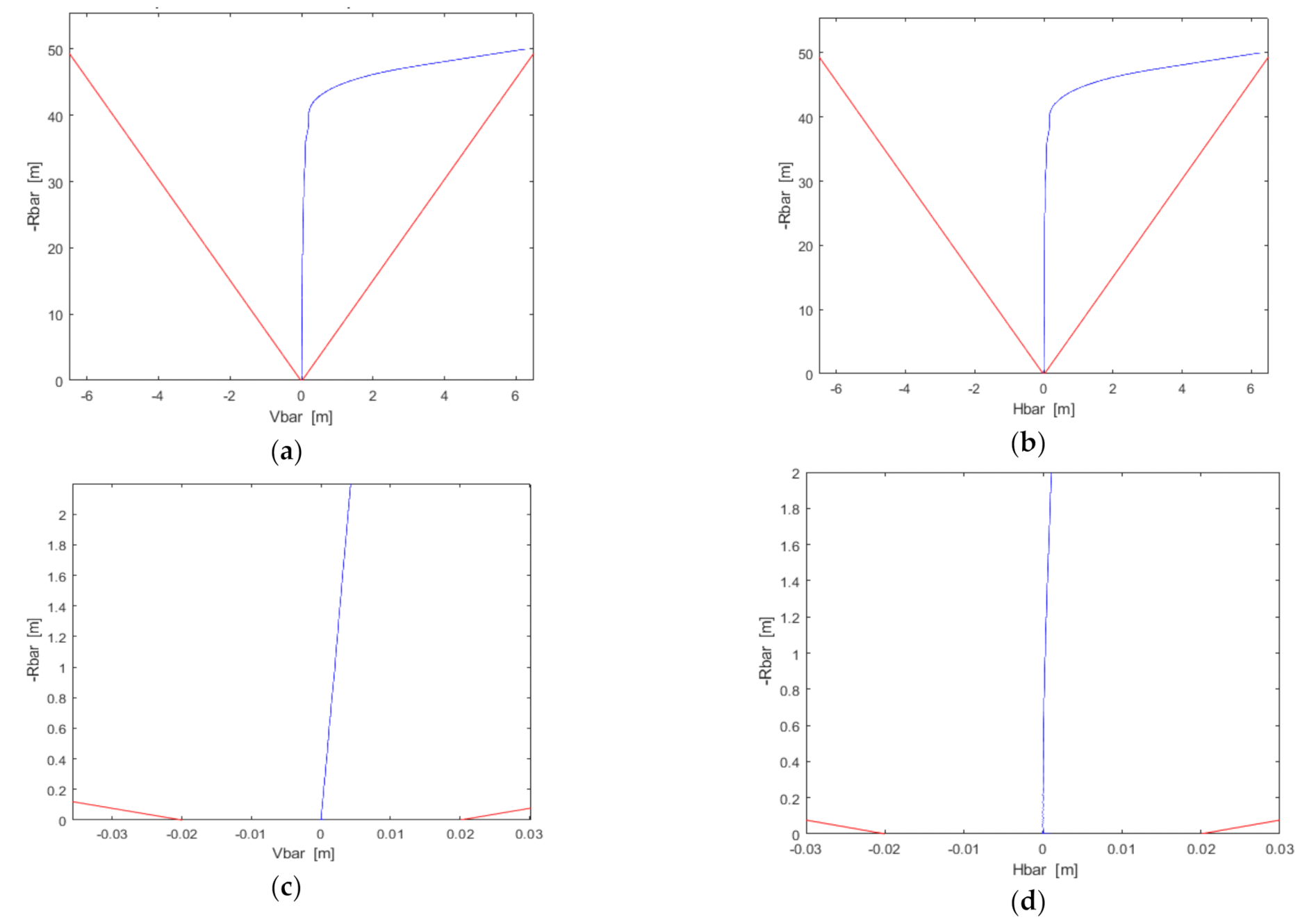
The simulation was performed under the worst initial conditions, i.e., initial Chaser position on the border of the approach corridor (x₀ = [+6.25, +6.25, −50] m), maximum Chaser initial velocity (V₀ = [0.2, 0.2, 0.2] m/s). These initial conditions are representative of one of the worst cases in the proposed scenario since it is considered that the Chaser starts to maneuver in proximity of the cone limits with a non-null velocity. The last part of the approach corridor (i.e., last 2 m) is restricted to a tube (rather than the cone) in order to check the real capability of tracking the reference immediately before the mating.

Figure 4 shows the trajectory in the H-bar-R-bar plane (Figure 4a) and V-bar-R-bar plane (Figure 4b), while Figure 4c,d details the trajectory in the last 2 m. The Chaser stays inside the tube limit with a distance of at least 1 cm, without risk of violation.

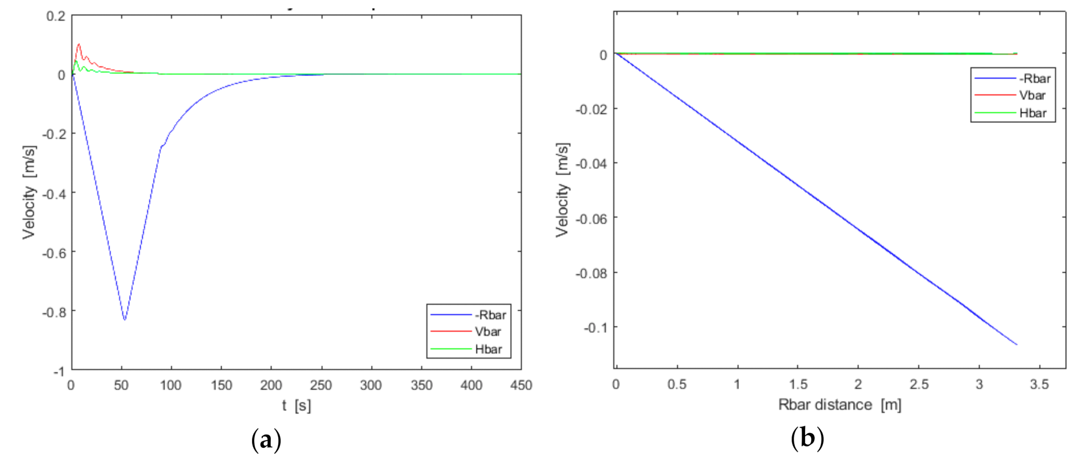
Figure 5a reports the trend in time of velocity along the three axes. The lateral velocity (i.e., along V-bar and H-bar) is always lower than 0.01 m/s and this value is observed in the first seconds of simulation and is due to the uncertainties on the initial conditions. Along the R-bar, the max velocity is around 0.8 m/s reached in the first phase of the maneuver since the controller leads the satellite to the desired reference straight-line as soon as possible. Then, the velocity is deeply reduced, and the approach velocity is less 0.1 m/s along the R-bar in the last 3.5 m (Figure 5b). The requirements on the approach velocity (see Table 1) are satisfied since the lateral velocity is 2 × 10⁻⁵ m/s and 3 × 10⁻⁵ m/s along the V-bar and H-bar, respectively, while the final approach velocity along the R-bar is 5 × 10⁻⁵ m/s.

Figure 6 reports the control efforts along the three axes. The maximum level of thrust, F_max, is not reached in the first 100 s and all the maneuvers for the docking are completed with a throttle ability of the 1% with respect to F_max. The time to complete the maneuver is 444 s.

The assessment of the control effort and the time to mating for different values of the matrix R of the TMPC has been conducted to refine the performance. The total control effort (T_c) is calculated as the sum of the absolute value of the control force along each axis for each step of simulation [25]:

$$T_c={\displaystyle \sum }_{t=0}^{tfin}\left|F_x\right|+\left|F_y\right|+\left|F_z\right|$$

(16)

Table 3. Control effort related to Equation (14).

R Matrix Values	Total Control Effort [N]	Time to Docking [s]
[10−2 10−2 10−2]	2.0260	491
[10−1 10−1 10−1]	2.0197	478
[1 1 1]	2.0470	464
[10 10 10]	2.0084	437
[102 102 102]	2.0450	468
[103 103 103]	2.0470	520

reports the results of the analysis on the control effort, that led to select the best values for R matrix.

It is worth noting that all the simulations ended with the satisfaction of the requirements in Table 1.

4.2. Robustness of the Solution

In this paragraph, the robustness of the TMPC is verified through the results of the 300 Monte Carlo simulations. Each simulation randomly varies for the initial conditions inside the range reported in

Table 4. Initial conditions of the simulation with the boundaries of uncertainties.

Parameter	Value	Uncertainties
Chaser mass $m_{ch}$	20 $\mathrm{kg}$	±20%
Target mass $m_{tg}$	2000 $\mathrm{kg}$
Chaser initial relative position $x_{ch0}$,$y_{ch0}$, $z_{ch0}$	$\left[0; 0;-50\right]$$\mathrm{m}$	±2.5 m
Chaser initial velocity $\dot{x}{ }_{ch0}, \dot{y}{ }_{ch0}, \dot{z}{ }_{ch0}$	$\left[0; 0; 0\right]$m/s	±0.2 m/s
Max force for each axis Fmax	35 mN

.

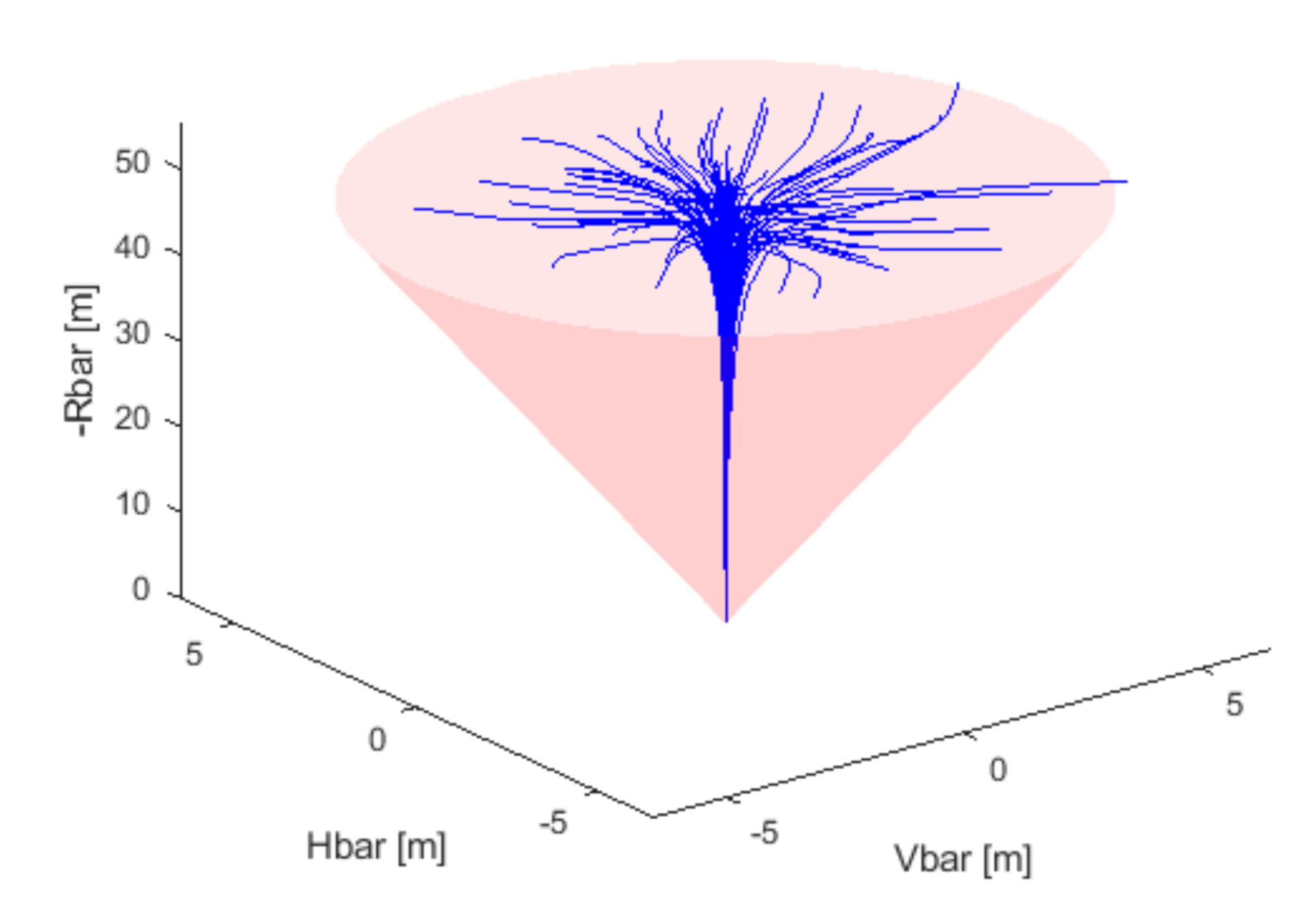
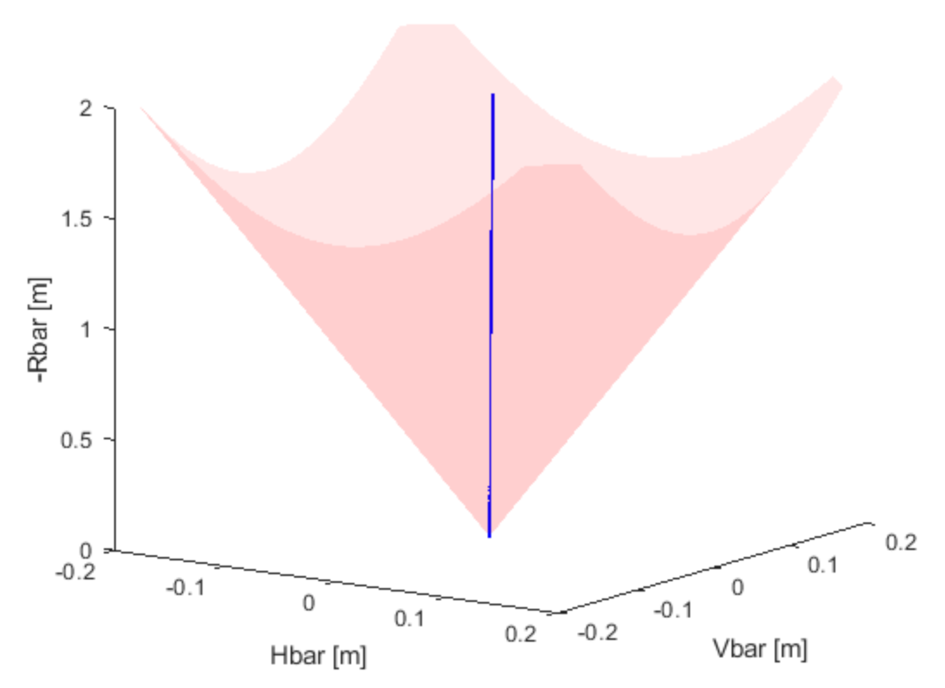
In Figure 7, the 3D trajectory is reported while the focus of the last 2 m is shown in Figure 8. These figures demonstrate that the uncertainties on the initial relative position and velocity do not avoid achieving in less than 30 m the desired reference straight-line trajectory, that is then maintained up to the mating. Note that all the trajectories are greatly inside the safety cone and cylinder.

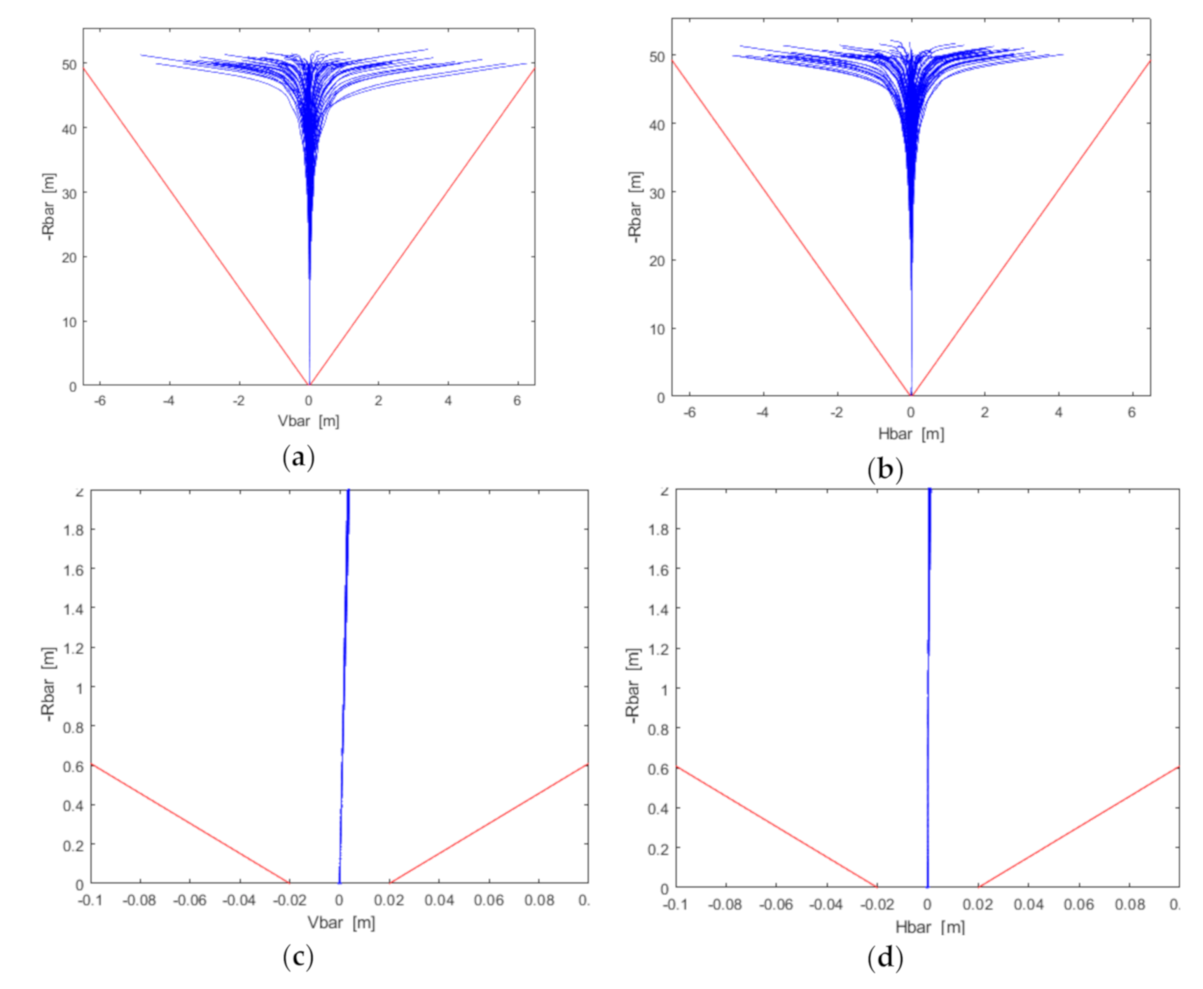
Figure 9 highlights the trajectory in the H-bar-R-bar plane (Figure 9a) and V-bar-R-bar plane (Figure 9b), while (Figure 9c,d) details the trajectory in the last 2 m, where the Chaser stays inside the cylinder limits with a distance of at least 1 cm, preventing the risk of violation.

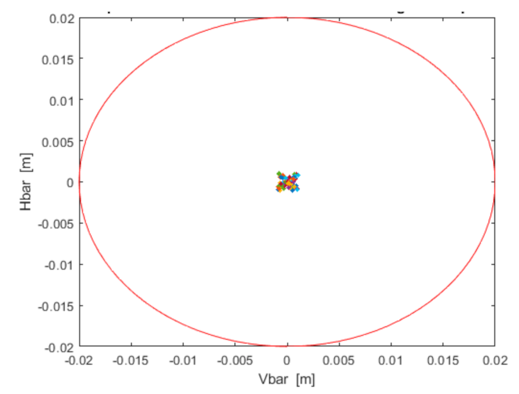
The rate of success to achieve the mating point inside the requirements (i.e., 2 cm) is 100% (as shown in Figure 10), i.e., the final lateral misalignment is less than 2 mm both with respect to V-bar and H-bar. The Monte Carlo simulation highlights how the accuracy on the mating point can slightly worsen and the small “bubble” around the ideal mating point (i.e., 0;0; 0) can be observed. This is due to the precision of the PWM used for the valves actuation that allows a minimum thrust of 35 µN. Improving the precision of the duty cycle, the “bubble” lessens and a higher accuracy is achieved.

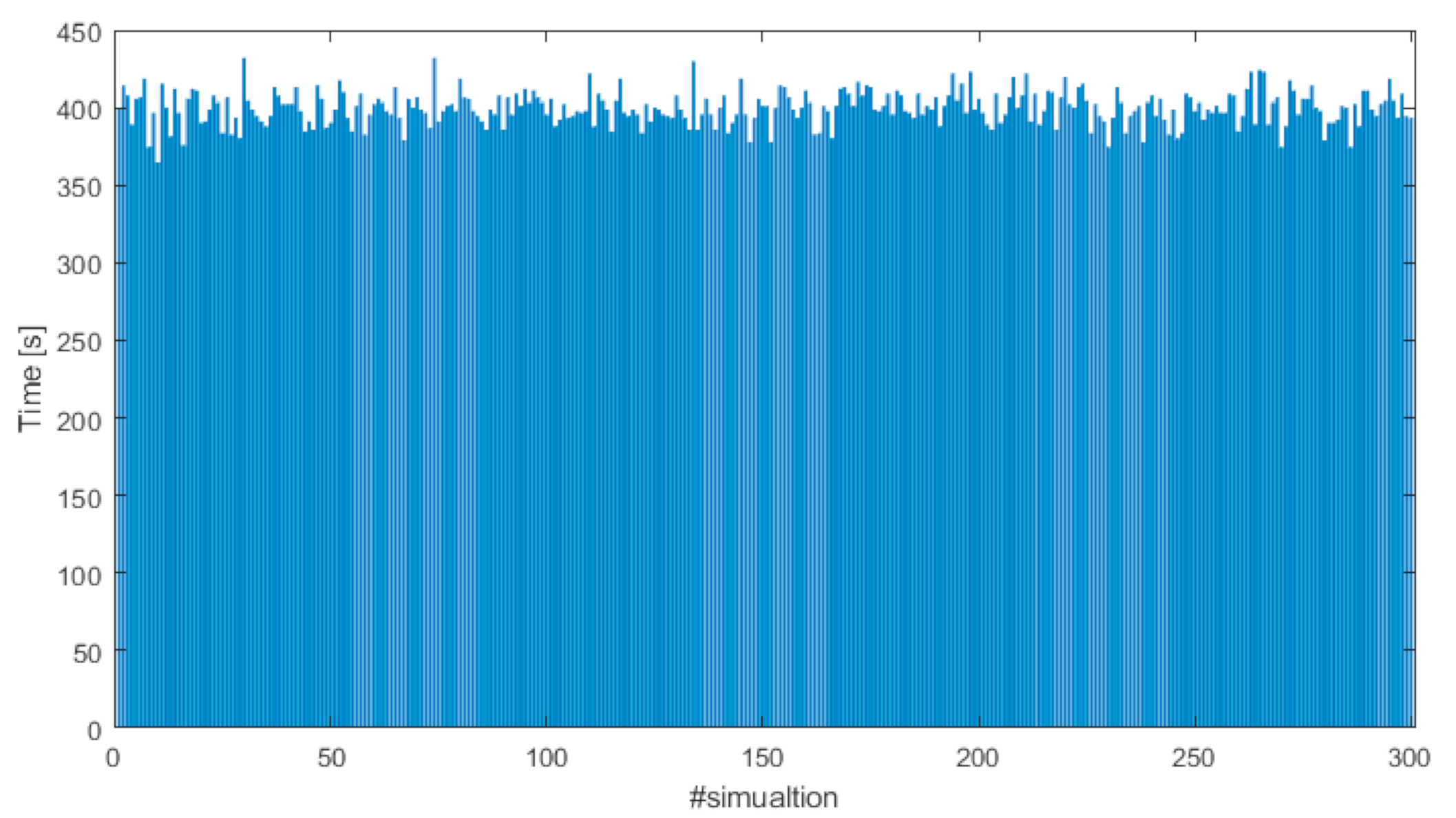
The conducted analysis includes the assessment of the time required to complete the docking maneuver and the control effort. The 300 Monte Carlo simulations show that the maneuver duration stays in the range [364, 433], as shown in Figure 11. Considering that the docking maneuvers should be performed when both spacecrafts are in visibility and in communication with at least one ground station, the reported values are compliant with the duration of the visibility window of a spacecraft in low Earth orbit over a ground station (that could be 10 min).

5. Conclusions

The docking phase for small satellites is very challenging due to the small dimensions of these spacecrafts and the performance of the available technology. This paper aimed at assessing the feasibility of the maneuvers to achieve the soft-docking performance in nominal conditions (i.e., without considering violations of the safety constraints and misbehaviors of the onboard systems that would lead to collision avoidance maneuvers) through the design and verification of a trajectory controller based on a linear tracking model predictive controller.

The tuning of the controller parameters is of paramount importance to achieve the optimal and robust performance. This performance is checked using a nonlinear model both for the analysis in the worst case and for the robustness analysis made through 300 Monte Carlo runs. It is demonstrated that the lateral misalignment at the mating point which is lower than 2 mm is achieved, the approaching velocity is lower than 1 mm/s, and the lateral velocity is deeply lower than 0.1 mm/s. The entire maneuver is completed in less than 10 min and with a reduced control effort. Moreover, the achieved results show that a relevant margin exists between the performance and the required values, ensuring that the capability of the system works properly in the presence of all the uncertainties and confirming the robustness of the controller. It is worth noting that the controller is tuned to robustly operate under the realistic assumption in which the docking phase (and the related maneuvers) start when the Chaser lies in proximity of a hold point at 50 m along the docking axis and, in any case of uncertainty on this position, the Chaser remains inside the cone approach. Moreover, the Chaser has reduced radial and lateral velocities and faces the Target.

In the future, the proposed solution will be extended considering that the docking port and the docking mechanism frames are not coincident with the body frames of the Target and Chaser, respectively. In addition, studies on the collision avoidance maneuvers will be conducted to evaluate the ability of the controller to react in case of off-nominal conditions. From the point of view of the controller, the TMPC architecture can be used to investigate other reference tracking strategies, for example, imposing a controlled velocity to reduce the velocity in the first part of the maneuver and to maintain a small but constant velocity for the soft docking reducing the maneuver time. Further in the loop simulations will be planned to investigate in detail the computational load of the algorithms.

References

- Kopacz, J.R.; Herschitz, R.; Roney, J. Small satellites an overview and assessment. Acta Astronaut. 2020, 170, 93–105. [Google Scholar] [CrossRef]
- Nichele, F.; Villa, M.; Vanotti, M. Proximity operations—Autonomous space drones. In Proceedings of the 4S Symposium, Sorrento, Italy, 29 May–3 June 2018. [Google Scholar]
- Corpino, S.; Stesina, F. Inspection of the cis-lunar station using multi-purpose autonomous Cubesats. Acta Astronaut. 2020, 175, 591–605. [Google Scholar] [CrossRef]
- Nastasi, K.; Thomas, D.; Tetreault, K.; Elliott, I.; Black, J. Real-Time Optimal Control, & Tracking of Autonomous. In Proceedings of the Micro-Satellite Proximity Operations, AIAA SPACE, Long Beach, CA, USA, 13–16 September 2016. [Google Scholar] [CrossRef]
- Gorret, B.; Métrailler, L.; Pirat, C.; Voillat, R.; Frei, T.; Collaud, X.; Mäusli, P.; Arato, L.; Lauria, M. Developing a reliable capture system for Cleanspace one. In Proceedings of the International Astronautical Congress, Guadalajara, Mexico, 27–30 September 2016. [Google Scholar]
- Corpino, S.; Stesina, F.; Calvi, D.; Guerra, L. Trajectory analysis of a CubeSat mission for the inspection of an orbiting vehicle. Adv. Aircr. Spacecr. Sci. 2020, 7, 271–290. [Google Scholar] [CrossRef]
- Pedrotty, S. Seeker Free-Flying Inspector GNC System Overview. In Proceedings of the 42nd AAS GNC Conference, Breckenridge, CO, USA, 1–6 February 2019. [Google Scholar]
- NanoACE—Gunter’s Space Page (skyrocket.de). Available online: https://space.skyrocket.de/doc_sdat/nanoace.htm (accessed on 22 July 2021).
- Leon, L.; Koch, P.; Walker, R. GOMX-4—The Twin European Mission for IOD Purposes. In Proceedings of the Small Satellite Conference, Logan, UT, USA, 4–9 August 2018. [Google Scholar]
- Roscoe, C.W.T.; Westphal, J.J.; Mosleh, E. Overview and GNC design of the CubeSat Proximity Operations Demonstration (CPOD) mission. Acta Astronaut. 2018, 153, 410–421. [Google Scholar] [CrossRef]
- Pirat, C.; Ankersen, F.; Walker, R.; Gass, V. Vision Based Navigation for Autonomous Cooperative Docking of CubeSats. Acta Astronaut. 2018, 146, 418–434. [Google Scholar] [CrossRef]
- Opromolla, R.; Fasano, G.; Rufino, G.; Grassi, M. A review of cooperative and uncooperative spacecraft pose determination techniques for close-proximity operations. Prog. Aerosp. Sci. 2017, 93, 53–72. [Google Scholar] [CrossRef]
- Sansone, F.; Francesconi, A.; Olivieri, L.; Branz, F. Low-Cost Relative Navigation Sensors for Miniature Spacecraft and Drones. In Proceedings of the 2015 IEEE Metrology for Aerospace (MetroAeroSpace), Benevento, Italy, 4–5 June 2015; pp. 389–394. [Google Scholar] [CrossRef]
- Branz, F.; Olivieri, L.; Sansone, F.; Francesconi, A. Miniature docking mechanism for CubeSats. Acta Astronaut. 2020, 176, 510–519. [Google Scholar] [CrossRef]
- Legostayev, V.P.; Shmyglevskiy, I.P. Control of space vehicles rendezous at the stage of docking. Automatica 1971, 7, 15–24. [Google Scholar] [CrossRef]
- Park, H.; Di Cairano, S.; Kolmanovsky, I. Model predictive control of spacecraft docking with a non-rotating platform. IFAC Proc. Vol. 2011, 44, 8485–8490. Available online: http://0-www-sciencedirect-com.brum.beds.ac.uk/science/article/pii/S1474667016449736 (accessed on 22 July 2021). [CrossRef]
- Li, Q.; Yuan, J.; Zhang, B.; Gao, C. Model predictive control for autonomous rendezvous and docking with a tumbling target. Aerosp. Sci. Technol. 2017, 69, 700–711. [Google Scholar] [CrossRef]
- Yang, H. Manned Rendezvous and Docking Technology. In Manned Spacecraft Technologies. Space Science and Technologies; Springer: Singapore, 2021. [Google Scholar] [CrossRef]
- Copot, C.; Muresan, C.I.; Beschi, M.; Ionescu, C.M. A 6DOF Virtual Environment Space Docking Operation with Human Supervision. Appl. Sci. 2021, 11, 3658. [Google Scholar] [CrossRef]
- Murtazin, R.; Sevastiyanov, N.; Chudinov, N. Fast rendezvous profile evolution: From ISS to lunar station. Acta Astronaut. 2020, 173, 139–144. [Google Scholar] [CrossRef]
- Arantes, G., Jr.; Komanduri, A.; Martins Filho, L.S. Guidance for rendezvous maneuvers involving non-cooperative spacecraft using a fly-by method. In Proceedings of the 21st International Congress of Mechanical Engineering, Natal, Brazil, 24–28 October 2011. [Google Scholar]
- Ueda, S.; Noumi, A. Precise Rendezvous Guidance in Low Earth Orbit via Machine Learning. In Proceedings of the 2019 SICE International Symposium on Control Systems (SICE ISCS), Kumamoto, Japan, 7–9 March 2019; pp. 27–32. [Google Scholar] [CrossRef]
- Li, P.; Zhu, Z.H.; Meguid, S.A. State dependent model predictive control for orbital rendezvous using pulse-width pulse-frequency modulated thrusters. Adv. Space Res. 2016, 58, 64–73. [Google Scholar] [CrossRef]
- Ventura, J.; Ciarcià, M.; Romano, M.; Walter, U. Fast and Near-Optimal Guidance for Docking to Uncontrolled Spacecraft. J. Guid. Control. Dyn. 2017, 38, 1–17. [Google Scholar] [CrossRef]
- Di Cairano, S.; Park, H.; Kolmanovsky, I. Model Predictive Control Approach for Guidance of Spacecraft Rendezvous and Proximity Maneuvering. Int. J. Robust Non Linear Control 2012, 22, 1398–1427. [Google Scholar] [CrossRef] [Green Version]
- Corpino, S.; Mauro, S.; Pastorelli, S.; Stesina, F.; Biondi, G.; Franchi, L.; Mohtar, T. Control of a Noncooperative Approach Maneuver Based on Debris Dynamics Feedback. J. Guid. Control. Dyn. 2017, 41, 431–448. [Google Scholar] [CrossRef]
- Calafiore, G.; Fagiano, L. Robust model predictive control via scenario optimization. IEEE Tran. Autom Control 2013, 58, 219–246. [Google Scholar] [CrossRef] [Green Version]
- Weiss, A.; Baldwin, M.; Erwin, R.S.; Kolmanovsky, I. Model Predictive Control for Spacecraft Rendezvous and Docking: Strategies for Handling Constraints and Case Studies. IEEE Trans. Control. Syst. Technol. 2015, 23, 1638–1647. [Google Scholar] [CrossRef]
- Bowen, J.; Villa, M.; Williams, A. CubeSat based Rendezvous, Proximity Operations, and Docking in the CPOD Mission. In Proceedings of the Small Satellite Conference, Logan, UT, USA, 10 August 2015. [Google Scholar]
- Pirat, C.; Ankersen, F.; Walker, R.; Gass, V. H-infinity and mu-Synthesis for Nanosatellites Rendezvous and Docking. IEEE Trans. Control. Syst. Technol. 2020, 28, 1050–1057. [Google Scholar] [CrossRef]
- Mammarella, M.; Lorenzen, M.; Capello, E.; Park, H.; Dabbene, F.; Guglieri, G.; Romano, M.; Allgöwer, F. An Offline-Sampling SMPC Framework with Application to Autonomous Space Maneuvers. IEEE Trans. Control. Syst. Technol. 2020, 28, 388–402. [Google Scholar] [CrossRef]
- Corpino, S.; Franchi, L.; Calvi, D.; Guerra, L.; Sette, S.; Stesina, F. Small satellite mission design supported by tradespace exploration with concurrent engineering: Space rider observer cube case study. In Proceedings of the 70th International Astronautical Congress (IAC), Washington, DC, USA, 21–25 October 2019. [Google Scholar]
- Chiesa, A.; Fossati, F.; Gambacciani, G.; Pensavalle, E. Enabling Technologies for Active Space Debris Removal: The Cadet Project. In Space Safety is No Accident; Sgobba, T., Rongier, I., Eds.; Springer: Cham, Switzerland, 2015. [Google Scholar]
- Stesina, F.; Corpino, S.; Feruglio, L. An in-the-loop simulator for the verification of small space platforms. Int. Rev. Aerosp. Eng. 2017, 10, 50–60. [Google Scholar] [CrossRef]
- Clohessy, W.H. Wiltshire, R.S. Terminal Guidance system for satellite rendezvous. J. Aerosp. Sci. 1960, 27, 653–658. [Google Scholar] [CrossRef]
- Xu, G.; Tianhe, X.; Chen, W.; Yeh, T.K. Analytical solution of a satellite orbit disturbed by atmospheric drag. Mon. Not. R. Astron. Soc. 2011, 410, 654–662. [Google Scholar] [CrossRef] [Green Version]
- Vadali, S. Model for Linearized Satellite Relative Motion about a J2-Perturbed Mean Circular Orbit. J. Guid. Control. Dyn. 2009, 32, 1687–1691. [Google Scholar] [CrossRef]
Figure 1.
Schematic of the reference frames.
Figure 2.
Safety corridor constraints: (a) xy plane, (b) xz plane, (c) yz plan.
Figure 3.
Simulation architecture.
Figure 4.
2D trajectory in (a) H-bar-R-bar plane and (b) V-bar-R-bar plane, and the detail of the last 2 m in (c) H-bar-R-bar plane and (d) V-bar-R-bar plane (worst case).
Figure 5.
Relative velocity (a) along the three axes vs. time, (b) in the last 2 m.
Figure 6.
The control effort for the worst case at the initial conditions.
Figure 7.
The 3D relative trajectory with the cone constraints.
Figure 8.
Focus on the 3D relative trajectory in the last 2 m with the cylinder constraint.
Figure 9.
The 2D trajectory in (a) H-bar-R-bar plane and (b) V-bar-R-bar plane, and the detail of the last 2 m in (c) H-bar-R-bar plane and (d) V-bar-R-bar plane.
Figure 10.
Accuracy at the mating point.
Figure 11.
Docking maneuver duration in the 300 Monte Carlo simulations.