Review

A Comprehensive Survey on Climate Optimal Aircraft Trajectory Planning

1
Department of Aerospace Engineering, Universidad Carlos III de Madrid, 28911 Leganés, Spain
2
Deutsches Zentrum für Luft- und Raumfahrt (DLR), Institut für Physik der Atmosphäre, Oberpfaffenhofen, 82234 Weßling, Germany
3
Faculty of Aerospace Engineering, Delft University of Technology, 2629 HS Delft, The Netherlands
4
Institute of Air Transportation Systems, German Aerospace Center, 21079 Hamburg, Germany
5
Institute of Air Transportation Systems, Hamburg University of Technology, 21079 Hamburg, Germany
*
Author to whom correspondence should be addressed.
Submission received: 20 January 2022 / Accepted: 25 February 2022 / Published: 7 March 2022

Abstract

:
The strong growth rate of the aviation industry in recent years has created significant challenges in terms of environmental impact. Air traffic contributes to climate change through the emission of carbon dioxide (CO2) and other non-CO2 effects, and the associated climate impact is expected to soar further. The mitigation of CO2 contributions to the net climate impact can be achieved using novel propulsion, jet fuels, and continuous improvements of aircraft efficiency, whose solutions lack in immediacy. On the other hand, the climate impact associated with non-CO2 emissions, being responsible for two-thirds of aviation radiative forcing, varies highly with geographic location, altitude, and time of the emission. Consequently, these effects can be reduced by planning proper climate-aware trajectories. To investigate these possibilities, this paper presents a survey on operational strategies proposed in the literature to mitigate aviation’s climate impact. These approaches are classified based on their methodology, climate metrics, reliability, and applicability. Drawing upon this analysis, future lines of research on this topic are delineated.

1. Introduction

The aviation sector plays an important role in international mobility. Currently, aviation is responsible for about 3–5% of total global warming [1]. The air transport industry is expected to thrive worldwide, rating 4.4% yearly and over the next 20 years. The influential parameters causing this development are, e.g., global population growth, metropolitanization, marketing expansions, as well as technological evolution [2]. Such a growth rate leads to a critical increase in environmental impacts. The aviation-induced climate impact consists of carbon dioxide (CO2) emissions and of non-CO2 effects. The non-CO2 effects comprise nitrogen oxide (NOx) emissions that are causing a concentration change in ozone and methane, water vapor emissions, aerosols, and persistent contrail and contrail-cirrus formation. CO2 and non-CO2 effects induce a change in the Earth’s radiation balance between incoming solar radiation and thermal outgoing radiation. This radiative imbalance is referred to as radiative forcing (RF). The overall global aviation RF of non-CO2 effects is positive and thus warming [3]. Moreover, it is important to note that non-CO2 emissions are responsible for two-thirds of the global aviation RF [1,4].
The technical core of the Single European Sky (SES) initiative launched in 2004 by the European Commission, is SES Air Traffic Management (ATM) Research Joint Undertaking (SESAR JU), that aims, among other objectives, to double airspace capacity whilst reducing the impact on the environment by 5–10% by 2035 [5], and achieving carbon neutrality by 2050. To tackle this challenge, we rely on the continuous development of more efficient aircraft, the use of alternative fuels or novel propulsion (i.e., mainly reducing CO2 effects (it can also be beneficial to reduce emissions such as NOx and soot)), and the avoidance of climate-sensitive regions at an operation level (i.e., reducing non-CO2 effects).
The introduction of more efficient solutions, mainly reducing direct CO2 emissions, is linked to implementation time scales of comparable magnitude to the contemplated horizon, associated both with the availability of new products within the aeronautical industry and the life cycle of current aircraft. The same applies to alternative propulsion. The feasibility of electric aircraft (all-electric or hybrid) in particular relies on technological enablers such as an increase in battery-specific energy. The specific energy density of the battery is estimated to increase by a factor of four for all-electric flights up to 500 nautical miles with 180 passengers on board [6], a factor which can be however reduced by resorting to a hybrid solution. Considering initially a short-haul application of electric aircraft, another key consideration directly affecting the profitability of this technology is charging time. Additionally, one has to consider the carbon intensity of electric energy generation. In [7], a hypothetical trend for the specific energy of batteries suggests that the viability of short-haul narrow-body hybrid aircraft eventually resides on a shift towards renewable energy production, nowadays requiring investment. Another alternative in the spotlight is hydrogen-powered aircraft, which do not emit CO2 but, in turn, emit more water vapor, which may lead to a higher formation of persistent contrails compared to kerosene-engine exhausts. To explore the mitigation potential of hydrogen aircraft, a better understanding of their climate impact due to contrail effects is required.
Alternative fuels, while having the benefit of running on existing engines, face a similar issue. Their successful contribution towards mitigating the climate impact of aviation relies on the sufficient availability of feedstock and refining industries, tied to the appearance of policy and price stimulation, as estimated in [8]. However, this study excludes the effect of non-CO2 emissions, the consideration of which results in significantly lesser mitigation [9]. Nonetheless, while the use of alternative propulsion, jet fuels, and the continuous improvement of aircraft efficiency present themselves as necessary developments towards the achievement of sustainable aviation, these solutions lack immediacy. Aside from large implementation time scales, they require substantial investment in research, production, testing, and certification. Consequently, employing alternative solutions that can bridge this time horizon is crucial. Here is where climate-friendly aircraft operations can make a difference.
In contrast to CO2 emissions, non-CO2 effects highly depend on the geographical location, altitude, time of day, and current spatial and synoptic conditions. By taking into account the dependencies of non-CO2 effects in the aircraft trajectory planning, operational mitigation towards climate optimized aircraft trajectories is possible. Thus, to consider the climate impact of aviation in the aircraft path planning, information on the climate-sensitive regions, i.e., regions where those non-CO2 effects are significantly enhanced, needs to be available. Moreover, aircraft dynamical models and the optimization approach are crucial factors affecting the performance and mitigation potential of the optimized trajectories. Numerous studies on climate-optimized trajectories exist. However, these studies differ, e.g., in the optimization algorithm, incorporation of climate impacts as the objective function, number of flights, and maneuvres. That is why our study aims to provide a comprehensive review of the state-of-the-art studies for the past two decades, i.e., 2000–2021, considering these factors, e.g., aircraft dynamical model, climate metrics, and optimization approaches. Of course, there exist some valuable surveys. For example, there are two surveys on the methods adopted for aircraft trajectory optimization (ATO) [10,11], and there is another review on contrail avoidance techniques [12]. Additionally, climate mitigation strategies were partially reviewed in the study of Zou et al. in 2013 (online version) [13]. The most recent survey, considering the time period 2000–2018, was conducted on the mathematical optimization in enhancing the sustainability of aircraft trajectory [14]. Here, in addition to climate impacts, the authors also considered the effects of noise. However, the authors in [14] did not review the climate impacts of aviation in sufficient detail. For instance, only two studies regarding contrail mitigation strategies were reported, and also the focus was on optimal control and meta-heuristic as solution approaches. Nevertheless, at the time of publication of the above-mentioned survey, some additional papers had investigated the reduction of contrail induced climate impacts, and used different techniques, including path planning and mathematical programming, to mitigate climate impacts of non- C O 2 emissions. In our proposed survey, this review is conducted so that all the mentioned aspects regarding climate impacts of non- C O 2 emissions and solution approaches are addressed in detail. After reviewing recent studies, existing scientific gaps are identified to propose a future road map of eco-efficient flight planning.
The rest of the paper is arranged as follows. In Section 2, the motivation of this survey is provided by presenting the climate impact of non- C O 2 emissions and how they can be mitigated using operational strategies. In Section 3, the optimization-based mitigation strategies, including optimal control and non-optimal control approaches, are presented. In Section 4, the recent studies in the literature are reviewed through the classification proposed in Section 3. Challenges and scientific gaps are discussed in Section 5 and a future road map is proposed. Section 6 closes the paper by presenting some concluding remarks.

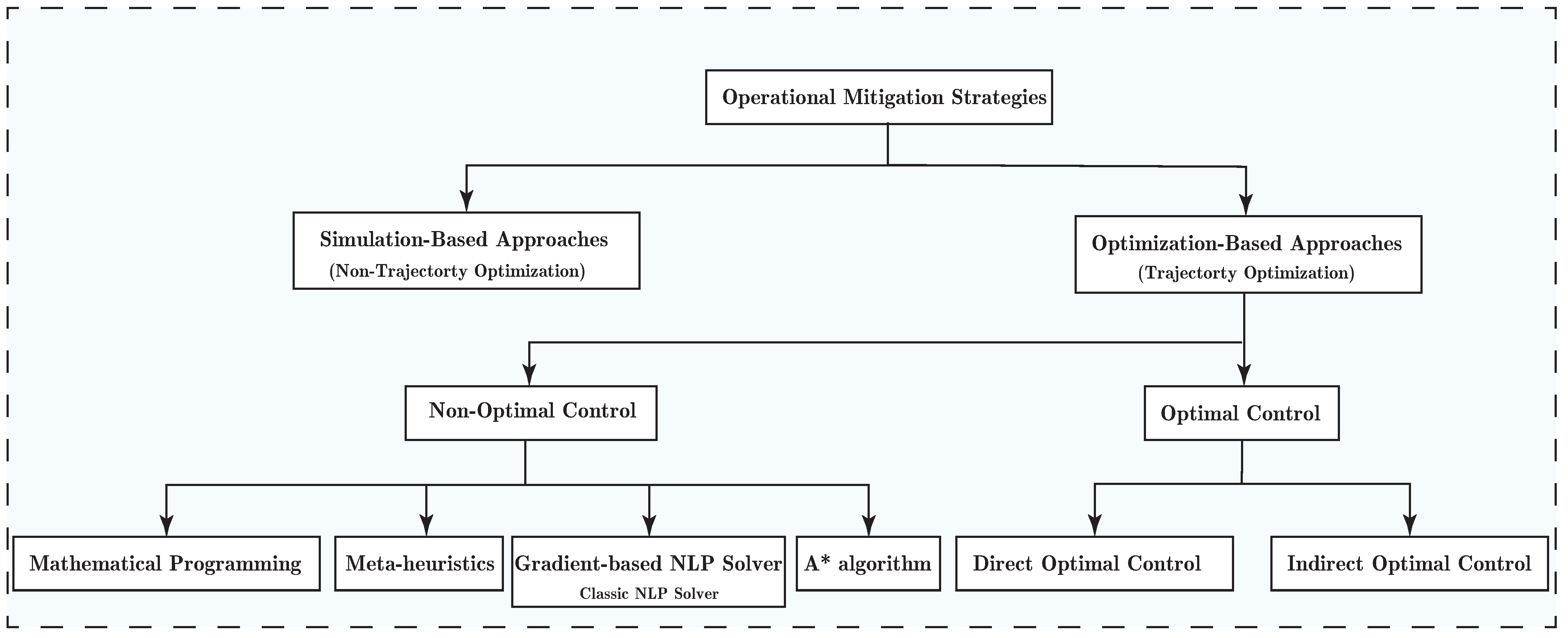
2. Operational Mitigation Strategies for non-CO2 Climate Impact

This section describes the climate impact of non- C O 2 emissions and the potential to mitigate their effects by employing operational routing strategies. Then, various published state-of-the-art approaches used as operational treatment are briefly presented.
Recently, state-of-the-art C O 2 and non- C O 2 RF estimates from global aviation (1940 to 2018) were reported in [1], showing that non- C O 2 impacts comprise about two-thirds of the net RF. Thus non- C O 2 aviation emissions contribute to aviation-induced global warming to a large extent. A detailed overview of all individual RF effects, including C O 2 and all single contributions of the non- C O 2 effect is provided in [1]. Figure 3 of this study (i.e., [1]) shows that the total non-CO2 RF effect is mainly caused by contrail cirrus and N O x emissions. N O x emissions lead both to the chemical destruction of methane and to the chemical formation of ozone; however, the resulting net N O x effect is positive, as the ozone formation dominates. Overall the RF of contrail cirrus, in spite of its large uncertainty, has the largest contribution to positive net RF. Water vapor and aerosol–radiation interactions from soot particles are estimated to have a slight impact.
While C O 2 emissions are only related to fuel consumption, non- C O 2 emissions are highly dependent on the meteorological and chemical background. Consequently, non- C O 2 climate impacts vary significantly with geographic location, altitude, and time of the emission [15]. Taking into account the spatial and temporal dependency of non- C O 2 climate impacts, aircraft trajectories could be adopted in order to avoid atmospheric regions that are highly sensitive to aircraft emissions [16].

Operational Mitigation Strategies

From the operational point of view, the mitigation of aviation climate impact is achieved by modifying aircraft maneuvres to avoid areas where those non- C O 2 effects are significantly enhanced, called climate-sensitive regions (CSR). The maneuvres can be the change of departure time, cruise altitude, lateral path, speed profile, and combinations of them. Therefore, to select a proper climate-aware trajectory for aircraft, information regarding climate-sensitive regions needs to be available, allowing to evaluate trajectories in the sense of contribution to climate impact. Besides, the approach to determine eco-efficient trajectory based on the considered metric (i.e., representative of CSR) plays an important role in the net mitigation potential. Thus, to mitigate the climate impact of aviation using operational strategies, the following two questions may be considered:
  • How to integrate climate effects in aircraft trajectory planning?
  • Which methods to generate optimized trajectories considering an objective function expanded by climate effects?
The operational mitigation strategies for aviation’s climate impact can be classified into two categories: non-trajectory optimization (NTO) (or, in some cases, simulation-based) strategies and trajectory optimization (TO) techniques (see Figure 1). Within NTO methods, after analyzing the properties of the climate impact of non- C O 2 emissions, the route, time, or the altitude of flights are slightly changed, and the mitigation potential is explored (through simulating aircraft performance with trajectory predictors) (e.g., see [17,18]). As for trajectory optimization, optimization techniques are employed to determine the aircraft trajectory such that a cost function containing some user-defined objectives (i.e., climate impact in this case) gets minimized [19,20].
The first attempts within the operational context were carried out using NTO strategies to see how the climate impact of non- C O 2 emissions can be mitigated with the change of time or the place of emission (roughly from 1998) [21] (see Section 4.1 for the review of these studies). These studies showed promising mitigation potential within the operational concept. In this respect, planning aircraft trajectories in a more optimal and accurate manner attracted many researchers from 2009. In fact, such strategies aim at finding the best possible and admissible trajectory among a wide range of options that meets some user-defined objectives. In other words, for instance, within simulation-based strategies, we might mitigate the climate impact of aviation by reducing 2000 ft of the flight level, but it may not be the best mitigation option. This is where optimal trajectories are more beneficial because, in such strategies, the optimizer seeks over possible trajectories by means of the employed optimization approach to select an optimal trajectory in the sense of considered objectives. The focus of this review is on TO methods, however, some NTO strategies are briefly reviewed in Section 4.1.

3. Trajectory Optimization

In general, optimization is the process of determining the best element among a set of feasible and available alternatives. In particular, trajectory optimization seeks the best possible trajectory of a dynamical system (e.g., aircraft dynamics in our case) in a finite-dimensional manifold with respect to some user-defined objectives as well as constraints and boundary conditions. Depending on the benchmark, there exist various classifications of trajectory optimization techniques (e.g., see [22,23]). This study aims to review and classify those methods focused mainly on mitigating aviation’s climate impacts in two categories: optimal control and non-optimal control approaches.

3.1. Optimal Control Approach

The optimal control (OC) is known as one of the most reliable dynamic optimization techniques since it works in continuous time, considers the system’s dynamical behavior, can provide analytic solutions to some types of problems, and adopts numerical methods. Within optimal flight planning, the aim is to determine feasible trajectories for aircraft considering practical constraints and the objectives specified by the flight planner.
One of the main features of optimal control over other mathematical optimization approaches is the consideration of the system’s motion along the time as dynamical constraints in the optimization process, allowing to achieve feasible transition of system. As generally considered within the optimal control framework, the time derivative of the system’s state is modeled as differential algebraic equations (DAE) in the following form [24]:
x ˙ ( t ) = f t , p , x ( t ) , u ( t )
where u R n u , x R n x , and p R n p are the vector of control inputs, states and algebraic variables, respectively and f is a vector field, mapping R × R n p × R n x × R n u R n . Equation (1) is continuous time representation of dynamical systems. The system can also be represented in discrete forms, which lie out of the scope of this paper (interested readers are referred to [25,26]).
In addition to the dynamical model of the system that is considered as differential constraints, some non-differential restrictions may be imposed over the whole time horizon, known as path constraints. Generally, these types of constraints are formulated as equality and inequality constraints, respectively as
h x ( t ) , u ( t ) , p , t = 0 g x ( t ) , u ( t ) , p , t 0
where h and g are the vector fields mapping h : R n x × R n u × R n p × R R n h and g : R n x × R n u × R n p × R R n g . 0 is a vector of zeros with appropriate dimensions, and the equality and inequality signs are applied in an element-wise manner. Besides path constraints, in a vast majority of optimization problems, some conditions are imposed on the initial and final values of state and control variables of the dynamic systems. Such constraints can also be considered as inequality and equality constraints, but in most cases, the equality one with restrictions only on state variables is used, which is defined as
Ψ t 0 , t f , x ( t 0 ) , x ( t f ) = 0
where Ψ : R × R × R n x × R n x R n ψ .
The optimal control theory seeks admissible control policies to optimize the performance of the system represented by Equation (1) with respect to some path and boundary constraints. Therefore, the optimization process needs an index to evaluate the performance. In control engineering, precisely, optimal control, such a cost functional is called the performance index. The objectives of the users should be mathematically interpreted and included in the performance index. The following general form of performance index is usually considered within OC problems, which is called Bolza [27]:
J i ( t 0 , t f , x , u ) = M t 0 , t f , x ( t 0 ) , x ( t f ) + t 0 t f L x ( t ) , u ( t ) , p , t d t
where M : R × R × R n x × R n x R and L : R n x × R n u × R n p × R R are continuously differentiable functions called terminal cost (or Mayer term) and running cost (or Lagrange term), respectively. If i = 1 , the optimization is a single-objective problem, and for i > 1 we have multi-objective optimization.
Finally, we can state a general form of the deterministic OC problem as: the determination of control policy u ( t ) R that minimizes the performance index Equation (4) with respect to dynamic constraints Equation (1), path constraints Equation (2) and boundary constraints Equation (3):
min u U J i ( t 0 , t f , x , u ) = M ( t 0 , t f , x ( t 0 ) , x ( t f ) ) + t 0 t f L t , x ( t ) , u ( t ) , p d t with respect to : x ˙ ( t ) = f t , p , x ( t ) , u ( t ) h ( x ( t ) , u ( t ) , p , t ) = 0 g ( x ( t ) , u ( t ) , p , t ) 0 Ψ ( t 0 , t f , x ( t 0 ) , x ( t f ) ) = 0
One can equivalently state this optimization problem as the determination of state, control, and algebraic variables that minimize the performance index and satisfy a set of dynamical, boundary, and path constraints. This is also true since, for instance, in numerical approaches such as direct collocation methods, the states of the system are also considered as decision variables [27,28].

3.1.1. Interpretation of Aircraft Trajectory Optimization as Optimal Control Problem

This section presents how, generally, aircraft trajectory can be optimized using OC problem formulation.

Dynamical Model of Aircraft

To efficiently simulate, predict and optimize the trajectory of aircraft, accurate models of dynamics that are capable of capturing its behavior in practice, while computationally inexpensive, are required. As an example, the following set of differential equations is associated with the full 4D point-mass model:
d d t ϕ λ h v t a s γ χ m = v t a s cos ( γ ) cos ( χ ) + w y R M ( ϕ ) + h 1 v t a s cos ( γ ) sin ( χ ) + w x R N ( ϕ ) + h cos ( ϕ ) 1 v t a s sin ( γ ) T ( C T ) D ( C L ) m 1 g sin ( γ ) L ( C L ) m · v t a s 1 cos ( μ ) g · v t a s 1 cos ( γ ) L ( C L ) sin ( μ ) m · v t a s cos ( γ ) 1 f c ( C T )
where λ is the longitude, ϕ is the latitude, h is the altitude, v t a s is the true airspeed, m is the mass, γ is the flight path angle, μ is the bank angle, χ is the heading, C T is the thrust coefficient, and C L is the lift coefficient. In addition, ( w x , w y ) are the components of the wind, R M and R N are the Earth’s ellipsoid radii of curvature in the meridian and the prime vertical, respectively, T, D, and L are the magnitudes of the thrust, drag and lift forces, g is the Earth’s gravity, f c is the fuel burn rate. As usually considered within the air traffic management studies, for computational purposes, the aircraft dynamical model represented by Equation (6) is reduced to more simplified models. For instance, by choosing directly the heading χ as a control, instead of the bank angle, the aircraft turn dynamics is disregarded, which would require more involved computations while in principle having little to no effect on the solution accuracy. A similar argument applies to the climb angle instead of, for instance, resorting to the lift coefficient.

Path and Boundary Constraints
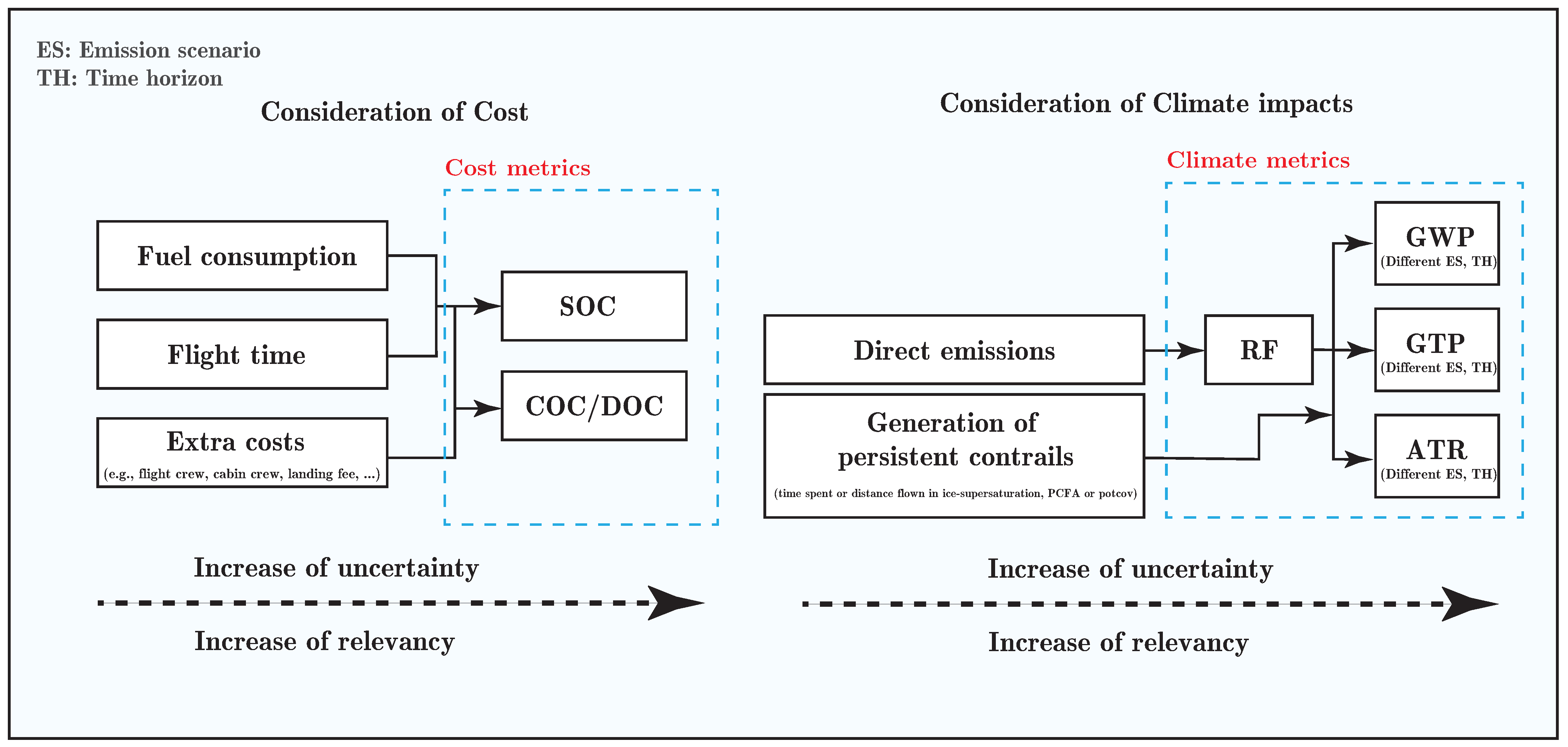
In addition to the dynamical model, a set of constraints is required for generating applicable and feasible trajectories. Initial and final values of states such as the geographical location of origin and destination, initial mass, and initial speed are some equality boundary constraints that are usually considered in ATO. Moreover, feasible ranges for speed profile and altitude can be interpreted as inequality path constraints.

Objective Function

Figure 2 shows the indices usually used for cost/climate optimal trajectory planning. Fuel consumption and flight time can be considered in the objective function. Besides, indices directly or indirectly considering climate impacts in terms of temperature change can also be regarded as other objectives.
To optimize aircraft trajectories, consideration of operating cost is a crucial aspect that needs to be addressed. This is due to the fact that today’s aircraft operations are designed and implemented based on minimum economical cost. There exist different definitions for cost in the literature, such as simple operating cost (SOC), presenting cost with linear relation to the flight time and fuel consumption, or via the so-called cash operating cost (COC), as a comprehensive economic criterion that considers different aspects of cost such as flight crew, cabin crew, landing fee, fuel, insurance, and maintenance for both airframe and engines [29] (see Table 1). In [30], such a definition of the cost is called direct operating costs (DOC). In the simplest cases, only flight time or fuel burn is considered as conflicting objectives to the climate impacts.
To consider the climate impacts of aviation, extra variables need to be included in the objective function (see Figure 2 right side). As non- C O 2 climate impacts are highly dependent on location and time of emissions, they can be mitigated with aircraft trajectory optimization if considered as objectives. However, the mitigation potential can vary with the climate metric employed for climate optimal trajectory planning. Possible indices used to enable climate optimal trajectory planning are briefly presented in the following (see Table 1). It is worth mentioning that the first two items, i.e., direct emission and persistent contrail formation are not climate metrics; however, they may indirectly lead to mitigating climate impacts (e.g., see [29], Table 4).
  • Direct emission: Some studies in the literature considered the emissions such as C O 2 and N O x in aircraft path planning [36]. Direct emission does not provide suitable insight into the climate impacts since, for instance, the effects of 1 kg emission of C O 2 on climate are highly different from that of N O x [33]. Instead, these emissions are usually inputted to other climate metrics to estimate the climate impacts caused by them. To calculate different emissions, the corresponding emission indices are required. There exist various approaches to calculate emission indices. Boeing fuel flow method 2 (BFFM2) is an extensively employed approach in the literature to calculate emission indices for N O x , CO, and HC [37,38].
  • Generation of persistent contrails: A great majority of studies focused on avoiding areas that are sensitive to the formation of persistent contrails (e.g., [39,40]). In these so-called ice-supersaturated regions (ISSR), the formation of persistent contrail cirrus is possible [41]. In some cases, in addition to the ISSR, Schmidt–Appleman criterion (SAC), stating the formation of contrails at sufficiently low temperatures and sufficiently moist (relative to liquid water) environments is adopted [42,43,44]. In the literature, the consideration of both ISSR and SAC is called persistent contrail formation areas (PCFA) [13]. Within the numeric global climate model, such areas can also be identified by means of potential contrail cirrus coverage, a fraction of the grid box which contrails can maximally cover under the simulated atmospheric condition [29,45,46]. Such fractional representation is mainly due to the relatively large grid box size within climate models. Usually, time or distance flown in contrail-sensitive areas is defined as the objective to be minimized. In addition, the areas that are favorable for contrails are inputted to those metrics that quantify their corresponding climate impact, as the condition, determining the existence of the contrails.
  • Radiative forcing: In some studies, RF has been used to quantify the climate impacts of aircraft emissions [47,48]. However, RF is not a direct measure of climate change. Instead, it measures the energy imbalance caused by changes in the Earth’s radiation balance between incoming solar radiation and thermal outgoing radiation. Such radiative impact has the potentiality to evolve the atmosphere temperature, estimated by RF [33].
  • Global warming potential: One climate metric that allows comparing the climate impacts of all agents (i.e., greenhouse gases) is the global warming potential (GWP) [34,49]. GWP estimates how much energy (calculated using time-integrated RF) is absorbed for the emission of a trace gas compared to that of 1 kg carbon dioxide ( C O 2 ) over a given period. Thus, the larger the GWP, the more a given gas warms the earth in relation to C O 2 over that period. Depending on the objective and application, some factors need to be considered to define suitable metrics. For instance, the emission scenario (e.g., pulse, sustained, or future emission scenario) and time horizon (e.g., 20 years or 100 years) are to be specified. The sustained emission scenario assumes constant emission of gas for the considered period, while pulse emission regards the emission of gas for one year and zero thereafter. The time period is specified with the selection of the time horizon. The studies [33,34,49] have discussed the selection of these factors based on different objectives. As an example, the pulse emission scenario for the time horizon of 20 years can be a suitable option for representing the short-term climate impacts. In contrast, 50 and 100 years time horizons can be used to capture medium-range and long-term climate impacts, respectively.
  • Global temperature change potential: Unlike the GWP, estimating heat absorbed over a given period caused by a greenhouse gas emission, global temperature change potential (GTP) provides the temperature change at the end of the period [34]. This metric adapts a linear system for modeling the global temperature response to aviation emissions and contrails. In this metric, similar to the GWP, the changes are estimated compared to C O 2 . For the GTP, the emission scenario and the time horizon need to be specified.
  • Average temperature response: Another metric that measures the climate impact in terms of temperature change is average temperature response (ATR) [33,49]. ATR is a derivative metric of GTP which combines the integrated temperature change for different emission scenarios and time horizons. Some functions (called climate change functions) have been developed within the EU-projects REACT4C, ATM4E, and FlyATM4E to quantify the climate impacts of each agent in terms of ATR. In Section 4, the employment of such functions for climate optimal trajectory planning will be reviewed.
The climate impacts can also be quantified with different derivatives of GWP, GTP, and ATR, such as mean GTP (MGTP) and absolute GTP (AGTP) [50].
In the studies that will be reviewed in Section 4, one can see that these indices, combinations, or conversions of them have been used in the literature for determining climate optimal trajectories. For instance, in [32], the GWP is converted to a monetary cost, or in another study, PCFA is used for considering contrails effects, and GWP is used for the remaining agents (i.e., N O x , C O 2 , and H 2 O emissions) [51].
As can be seen in Figure 2, some of the indices are inputted to other more relevant ones. For instance, time and fuel are used to represent SOC (usually expressed in USD [29]), or in the case of climate impacts, emissions are taken to calculate the corresponding warming potential or temperature changes. It should be noticed that, despite increasing relevancy, they may lead to more uncertain quantification of impacts [33,34].

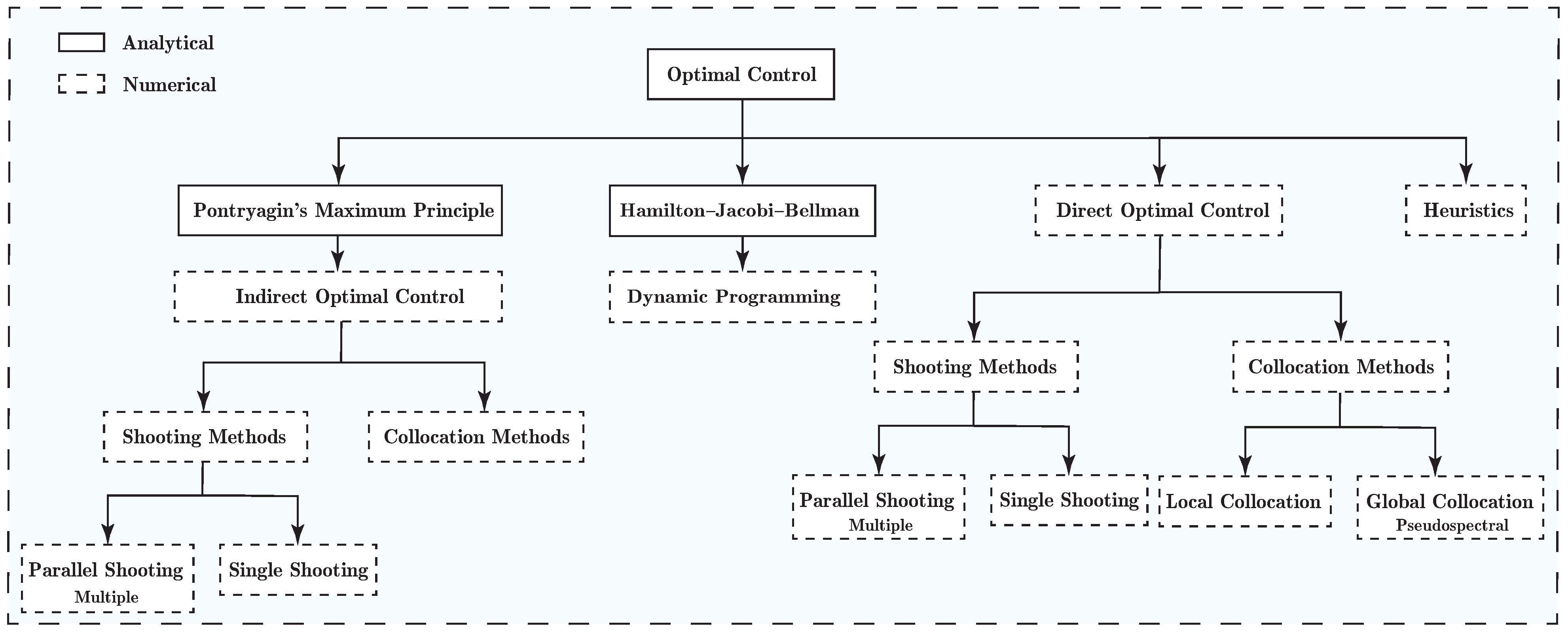
3.1.2. Solution Approaches

There exist various approaches in the literature to solve the optimal control problem formulated in the previous section. However, to select the suitable one, some factors need to be considered. Depending on the structure of the control policy (i.e., closed-loop and open-loop), online (e.g., receding horizon) and offline, level of optimality (e.g., sub-optimal and optimal or local and global solutions), type of the dynamical system (e.g., linear or nonlinear, number of state and control variables), the form of the cost functional (e.g., linear, quadratic, or nonlinear), constraints, time horizon (i.e., infinite or finite), and computational time, the applicability of these methods changes.
One classification of optimal control methods can be based on how they solve the optimization problem, i.e., analytically or numerically. Theoretically, Pontryagin’s minimum principle (PMP) and the Hamilton–Jacobi–Bellman (HJB) equation are the two main approaches that characterize optimal solutions to the OC problem. The former provides the necessary conditions for optimality, while sufficient conditions are obtained from HJB. As for the numerical approaches, we have indirect and dynamic programming methods utilized to solve the problems obtained using PMP and HJB numerically, and the direct approach, which directly attempts to solve the OC problem by converting the original infinite-dimensional problem to a finite-dimensional one (i.e., nonlinear programming (NLP)), called transcription. Figure 3 shows a classification of optimal control methods used to solve ATO problems. In Appendix A, these methods are briefly presented.

3.2. Non-Optimal Control Approach

Non-optimal control methods try to solve dynamical optimization problems in a more simplified manner. Some of the simplifications commonly assumed within these techniques are disregarding aircraft dynamics and constraints or considering them in a streamlined way, such as linearized ones. These methods aim to provide fast and, to some extent, reliable solutions, even if not resulting in the best trajectories. To tackle such optimization problems, various approaches, such as geometric methods, path-planning algorithms (e.g., well-known A * and D * algorithm), combinatorial optimization, and meta-heuristics are usually employed [52]. Within these methods, the optimization problem is formulated normally without considering aircraft dynamics or considering it partially to predict the performance of trajectories such as speed, fuel burn, emission indices, and climate impacts. Then, by making use of optimization techniques, the formulated problem is solved. For instance, if the trajectory of an aircraft is given as a sequence of discrete or/and continuous variables, and its performance can be quickly predicted, a suitable choice is a meta-heuristic approach, applying combinations of randomized heuristic procedures iteratively to enhance the candidate solution. Simulated annealing [53], genetic algorithms (GA) [54], variable neighborhood search [55], and particle swarm optimization [56,57] are some algorithms that are used as meta-heuristics solvers. Due to exploration and exploitation features, such algorithms are capable of providing approximate global solutions. In addition, they are not restricted to requiring gradient information and are straightforward to be implemented. Moreover, for such a class of problems, classical NLP solvers are beneficial to provide fast solutions. The main drawback of classical (or gradient-based) NLP solvers is the sensitivity to the initial guess, usually leading to local solutions.
The cost function of such optimization problems can be defined similarly in the sense of objectives to those within OC problem formulation. For instance, the Lagrange term of performance index may be approximated with a summation. Such methods are more beneficial when tackling the optimization for a high number of flights and also considering air traffic complexity (e.g., conflicts). Mathematical programming, A * algorithm, meta-heuristics, gradient-based NLP solvers such as successive quadratic programming (SQP), and interior-point are non-optimal control methods that have been employed in the literature to solve the climate optimal trajectory planning problem.

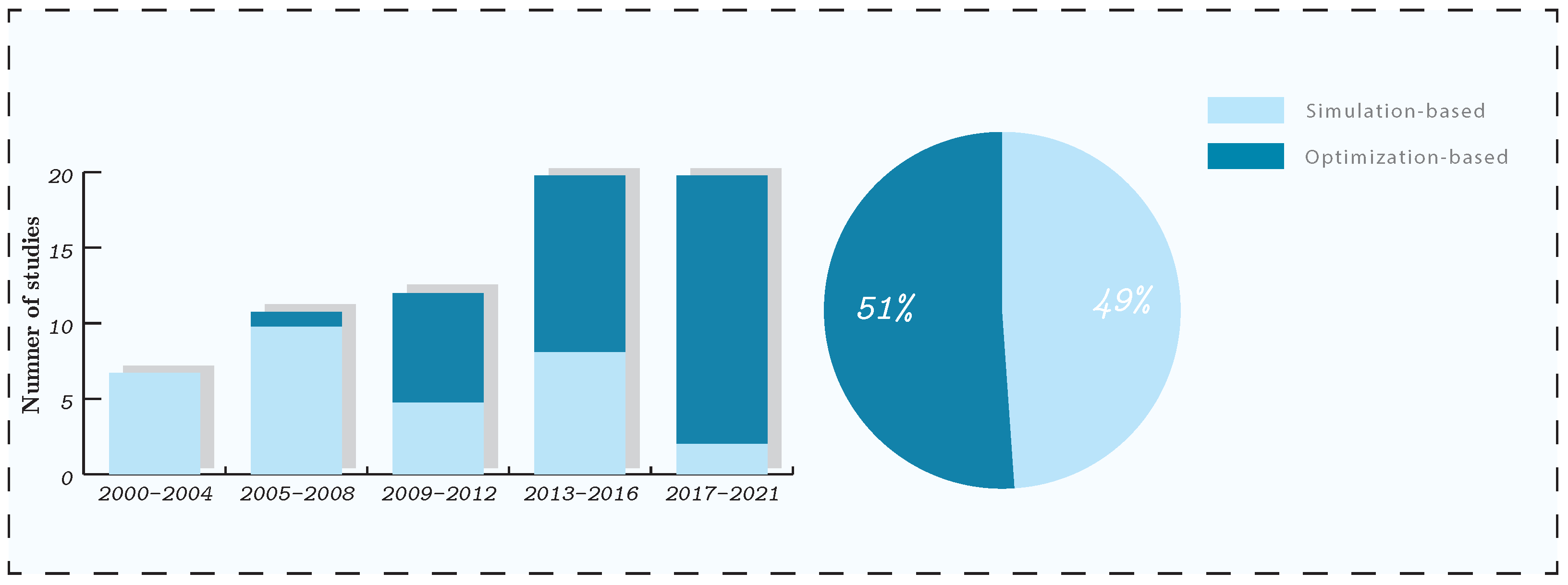
4. Review of Climate Optimal Trajectory Planning Studies

This section reviews the recent studies considering two main items: climate metrics and optimization approaches. The review of recent studies is based on employed operational strategies, and the climate metrics will be discussed for each study. Although the main focus is on reviewing trajectory optimization methods, some simulation-based (or NTO) techniques are presented as well (in Section 4.1). Figure 4 shows a comparison between simulation and trajectory optimization approaches using the number of studies reported in the literature.

4.1. Simulation-Based Strategies

In this section, we briefly review the first attempts made using NTO strategies. As presented in Section 2, within the NTO approach, the aircraft profile is slightly modified for different cases, and the mitigation potential is studied.
Myhre and Stordal [58] identified that flying the peak traffic periods during sunrise and sunset would be beneficial to reduce the climate impact of contrails. This is due to the amount of solar radiation reflected by the contrails being higher and, to some extent, can compensate for the warming impact of the trapped earth-emitted radiation.
Altering the cruise altitude is another alternative that has been studied numerously in the early studies in this field. In [59], it was shown through air traffic control mathematical simulator (RAMS) applied to European airspace that by restricting the cruise altitude to prevent the formation of contrails determined using potential contrail coverage, it is possible to mitigate the climate impacts by accepting an increase of only 4% in fuel burn and maximally one minute’s delay in arrival time. The seasonal cycle analysis was also performed, and the limit of maximum cruise altitudes was determined with respect to the potential contrail fraction of 5% (calculated using the approach in [60]) for different months. In the summertime, the highest allowable altitude was obtained at 31,000 ft. The authors also extended their analysis to the long haul flights by focusing on the North Atlantic and US airspace [17]. In the later study, the authors improved their results by considering short-term variability (6 h period) in the atmospheric conditions (instead of using monthly values over the whole day) of contrail coverage and proposed adaptive altitude restrictions for each period within the month [18]. The latter approach was more efficient due to the high variability of contrail formation with respect to time.
The effects of changing cruise altitudes on contrail coverage and its corresponding RF were investigated linked to the European Fifth Framework Project TRADEOFF [61]. It was reported that by decreasing the cruise altitude by 2000 ft, 4000 ft, and 6000 ft, the global annual mean of contrail coverage reduces approximately linearly with the maximum reduction of almost 45% for 6000 ft downshift of altitude. This study showed that the relative changes of corresponding RF are very similar to those of contrail coverage. They observed a substantial regional and seasonal variability in the contrail coverage and corresponding RF with the altitude change. Mannstein et al. suggested the development of a flexible free flight and the on-board detection of ISSR to change altitude in a real-time manner [12]. They reported that the contrail formation avoidance, in this case, would be achieved only by a slight change in flight altitude and, thus, more beneficial to the operating cost.
In addition to the vertical profile, Klima analyzed the effects of changing lateral paths to avoid the formation of contrails [62]. This study constructed different fuel-optimized aircraft trajectories considering various options for flying above, below, and around ISSR. The rerouted flights were considered for 581 continental flights between 14 city pairs and 628 international flights over the North Atlantic between 15 city pairs. The performance of the constructed trajectories was compared with the actual flights flown on a week of November 2011. The results showed a great mitigation potential in both persistent contrail formation and the fuel burn, which was approximately, on average, 72% and 6%, respectively.
Chen et al. used the contrail frequency index and investigated the effects of changing flight levels [63]. The persistent contrail formation was identified using the ISSR condition, and the contrail frequency index was defined as the multiplication of aircraft position to the ISSR. Their algorithm was performed to reduce contrails’ formation without adding congestion to airspace. They reported that reducing persistent contrail formation causes extra emission, and for pure contrail reduction strategy, it is possible to decrease the formation of contrail up to 88%. However, this value decreased when the trade-off factor with respect to emissions was taken into consideration. In this study, the emissions were modeled using a prototype of the Aviation Environmental Design Tool (AEDT) developed by the Federal Aviation Administration (FAA). BFFM2 was employed to calculate the emission indices of CO, HC, and N O x . The authors later extended their analysis by quantifying the climate impact of emissions using absolute global temperature potential (AGTP) and then expressing them as cost in dollars [64].
For the particular case of the EU-project REACT4C, within the study by Grewe et al., a strategy was proposed for 391 eastbound, and 394 westbound flights in the transatlantic region within the air traffic simulator (SAAM) [65]. SAAM is a tool allowing for creating, changing, and designing the air traffic route network with all possible associated constraints. For the case of conflict resolution, it employs a linear programming technique. The advanced emission model (AEM 2.5.0) was developed to estimate the mass and emissions for the generated 4D aircraft trajectories. The climate impacts were quantified by means of climate change functions (CCFs) developed using the European Center HAMburg general circulation model (ECHAM) and Modular Earth Submodel System (MESSy) and Modular Earth Atmospheric Chemistry (EMAC) models [66,67]. The EMAC model performs a numerical integration of the chemical and physical processes invoked by the emission of the different species, and the CCFs are five-dimensional data sets (longitude, latitude, altitude, time, type of emission), providing specific climate impacts, i.e., the estimated climate change for a local emission [49,68]. These CCFs, which model the climate impacts of N O x emissions, water vapor, and contrails, were developed for the North Atlantic region, considering a representative winter pattern. In [65], to analyze the climate impacts, different climate indicators with different emission scenarios over different time horizons such as P-AGWP100, P-AGWP20, and F-ATR20 were investigated. The results revealed a great mitigation potential in which, with a neglectable increase in costs, i.e., 0.5%, a 25% decrease in climate impacts was achieved. In [69], a larger set of weather patterns, including respectively five and three representative patterns in winter and summer, were analyzed for the CCFs. In [70], these weather patterns for CCFs were employed in SAAM considering flights similar to [65]. It was reported 1% increase in the cost could decrease the climate impact by 10%.
The mentioned approaches were efficient in the sense of reducing the climate impact of aviation. In fact, these studies provide a valuable understanding of operational strategies to mitigate the climate impact. However, it is worth mentioning that they are not the most optimized ones. This is because, in these studies, only some maneuvers (e.g., change of flight altitudes or routes) are simulated, and then suitable profiles are selected. Consequently, there exists a wide range of scenarios that are not taken into consideration. As a result, an operational approach that can select the best feasible trajectories (the best option in the view of the user, e.g., climate impact in this case) over all possible trajectories would be more efficient. To this end, from 2008, the researchers have been attracted to determine the aircraft trajectories in an optimal manner. In Section 4.2 and Section 4.3, optimization-based strategies will be reviewed. It is important to note that some simulation-based strategies are suitable for analyzing the climate impacts of numerous flights or scenarios, while in these cases, TO techniques, especially those within the optimal control approach, generally suffer from the computational perspective.

4.2. Non-Optimal Control Methods

As for the trajectory optimization techniques, we first start with non-optimal control approaches, which are usually less accurate compared to optimal control methods, but some of them are able to generate optimized trajectories in a fast and reliable manner. Table 2 summarizes the studies in the literature employing non-optimal control methods for climate optimal trajectory planning.

4.2.1. Mathematical Programming

Within the mathematical programming approach, the TO problems are approximated to be optimized using mathematical programming methods.
The first attempt considering climate impact as an objective to be minimized was made by Campbell et al. using mixed-integer programming (MIP) to avoid ISSR [71]. It was reported that for a single flight from O’Hara International Airport to Los Angeles International Airport, by adopting a 2.76% increase in fuel burn, the formation of persistent contrails could be completely avoided. In this study, the difference between employing mixed-integer linear programming (MILP) and mixed-integer quadratic programming (MIQP) for solving the optimization problem was explored. It was reported that MLQP provides more efficient trajectories; however, it required excessively higher computational time. The effects of planning horizon length and time step size within the receding horizon algorithm on the determined trajectories were also discussed. The authors in the next study [19], added a more realistic feature to their trajectory optimization technique, in which, instead of precluding flights from flying ISSR, these regions were modeled as soft constraints and included in the objective function with a penalization. For the same scenario as the previous study (i.e., [71]), it was reported that with an approximately 50% decrease in forming persistent contrails, the fuel burn increased by 1.48%. The aircraft dynamical model in these studies was not considered in an accurate manner, and a linear approximation was used to represent aircraft behavior. In addition, the impacts of wind on the aircraft trajectory were not considered, and the potential fuel savings that can be achieved by flying wind-optimal paths were neglected. Moreover, the different sets of parameters and settings in these methods yielded different solutions; thus, their approach was highly sensitive. The computational time to result in more accurate solutions while handling many obstacles and dynamic constraints was extensively high.
Wei et al. used the contrail frequency index similar to the approach proposed in [63] and examined the effects of changing flight levels on climate impacts [72]. Their algorithm was performed such that flying in areas favorable to produce persistent contrails reduces without adding congestion to airspace using linear programming. In spite of higher contrails formation compared to the similar study [63] (which is a simulation-based strategy), this study yielded better performance in terms of capacity by restricting shifted aircraft at each flight level.
Campbell et al. proposed an on-board trajectory planning strategy using mixed-integer linear programming (MILP) to find optimal trajectories with respect to fuel consumption and formation of persistent contrail [73]. Similar to the previous studies, ice-supersaturation was considered as the condition for persistent contrails (i.e., ISSR). For a single-flight scenario, an analysis of the same route for 20 days showed that by accepting an increase of 0.48% in fuel, 58% of persistent contrails could be avoided. Just as in their previous studies (i.e., [19,71]), the effects of wind were not considered, and a linearized aircraft model was employed to represent the aircraft behavior.
Zou et al. proposed 4D trajectory optimization (with constant speed) using the binary integer program [13]. In this study, for the first time, the climate impact of contrails was quantified using the GWP indicator. To make results comparable, all the factors were converted to monetary costs (in dollars), including fuel, crew, passenger travel time, C O 2 emission, and contrails. By using a successive optimization algorithm, the results were extended to multiple flight scenarios, considering the resolution of probable conflicts. It was reported that the optimal trajectory depends highly on the time horizon selected for calculating the climate impact of C O 2 .

4.2.2. Meta-Heuristics

Meta-heuristics approaches are employed when the trajectory of an aircraft is represented as a sequence of decision variables, and its performance can be quickly predicted.
Celis et al. proposed a 3D trajectory optimization technique based on GA and considered flight time, fuel burn, and N O x emission as optimization objectives [36]. The route, altitude, and true airspeed were considered on four segments and optimized using GA with respect to the defined objectives. It was reported that the minimum N O x -emission trajectory caused a 10.4% reduction in N O x emissions while increasing flight time and fuel burn by 1.0% and 3.9%, respectively.
Yamashita et al. developed the first version of air traffic simulator AirTraf, as a submodel of the EMAC model in [77,78]. The aircraft trajectory optimization in this model is performed using the GA algorithm. In this approach, several decision variables (typically 11) are considered to represent the vertical and horizontal trajectory of aircraft. Then, (third-order) B-spline curves are used to represent trajectories smoothly using the coordinates (obtained from decision variables). Fuel consumption, speeds, emissions (using the DLR method [77]), and objective functions are calculated and evaluated on a number of segments generated arbitrarily between coordinates. The adaptive range multi-objective genetic algorithm (ARMOGA) developed in [79,80,81] is employed to solve the formulated optimization. Although the climate impacts were not considered in these studies (i.e., [77,78]), they were a basis for the next studies considering climate impacts. For instance, the trajectory optimization was performed using EMAC/AirTraf 1.0 to minimize the climate impact of ozone quantified using algorithmic climate change function (aCCF) in [76]. The CCFs developed within EU-project REACT4C [49] were computationally expensive and, consequently, inefficient for the real-time calculation of climate impacts required within the future climate-aware trajectory planning. To deal with computational time spent in the EMAC model simulations to derive the CCFs, within EU-project ATM4E (which stands for air traffic management for environment), an approximate version of CCF called algorithmic CCF (aCCF) was presented, representing a correlation of weather system at the time of emission and the respective climate effects [82]. The aCCFs are computationally more efficient and can be implemented by known aircraft trajectory optimization techniques. Thus, Yin et al. used aCCF to quantify the climate impact of ozone with ATR20 as the climate indicator [76]. It was shown that, by flying lower altitudes, the net RF due to climate optimal routing option is received 0.3 mW/m2 less than the cost-optimal one. The authors in [46], using the EMAC model coupled with AirTraf 1.0 and a contrail submodel, optimized flight time and the flight distance through contrail forming regions modeled using potential contrail coverage (potcov) (see [45] for the calculation of potcov).
Yamashita et al. [29,31] developed the second version of AirTraf (i.e., AirTraf 2.0), enabling aircraft trajectory optimization for nine different routing options. One of these routing strategies is the climate optimal one, which employs aCCFs to model climate impacts of C O 2 and non- C O 2 emissions based on ATR20. In the latter study, which investigates the climate impacts of flying in different weather patterns (in summer and winter), the authors reported that there is a potentiality to have cooling impacts within some weather patterns [31].

4.2.3. Path Planning

Within path planning methods, the space is discretized, and the optimal trajectory is determined through working with the generated network.
Foster et al. in [30] present a tool that is capable of optimizing aircraft trajectories considering economic and ecological objectives, called Toolchain for Multicriteria Aircraft Trajectory Optimization (TOMATO). In this study, C O 2 , N O x , CO, black carbon-based emissions are calculated and then represented in monetary indices using emission trading scheme (ETS) certificates. The tool uses the Compromised Aircraft performance model with Limited Accuracy (COALA) to model the aircraft performance [83]. Similar to many reviewed studies, ice-supersaturation was considered as the condition determining the existence of persistent contrails. Then, the climate impacts were measured using GWP. Direct operating cost (DOC) and GWP of all emissions and contrails were included in the objective function. The optimization algorithm is similar to the classic A * algorithm for the horizontal route. In the next studies [32,75], Rosenow et al. employed this tool to optimize multiple flight scenarios (13,584 flights). In these studies, the network complexity analysis using the number of conflicts as the metric was investigated. However, the attention was only restricted to compare the number of conflicts between the actually flown trajectories within the current structured airspace (obtained from EUROCONTROL Demand Data Repository (DDR2)) and the optimized trajectory considering the future free-route concept, and no resolution analysis was taken into account.

4.3. Optimal Control Methods

As presented in Section 3.1, optimal control methods solve the ATO problems formulated as dynamical optimization. In Appendix A, different OC methods used in ATO are briefly presented. Only direct and indirect approaches have been employed in the literature to determine climate optimal trajectories. Table 3 summarizes the studies in the literature employing optimal control methods for climate optimal trajectory planning. These studies will be reviewed in the following.

4.3.1. Indirect Optimal Control

Due to the difficulty in deriving analytical solutions using PMP, especially singularity analysis, simplified aircraft dynamics (e.g., 2D cases, optimizing only lateral path) have been considered in the literature for determining climate optimal trajectories using an indirect approach.
Sridhar et al. [20], for the first time, attempted to find climate-optimized trajectories by considering the effects of wind. In this study, PCFA was used to capture persistent contrails, and these areas were modeled as soft penalties in the cost functional of the optimal control problem. PMP method was then employed to solve the optimization problem with flight time, fuel burn, and the time spent in contrail formation areas as objectives. To solve the received 2PBVP numerically, the indirect shooting approach was implemented. The trade-off between the formation of persistent contrails and fuel consumption was explored for 12 city pairs in the continental United States. Without altitude optimization, the reduction in the flight time in PCFA was gradual with the increase in fuel burn. When the altitude was optimized, a 2% increase in fuel could decrease the total flight times in PCFA more than six times.
In a later study [84], the authors modified the Future Air Traffic Management Concepts Evaluation Tool (FACET) to include contrails for performing trajectory simulation and optimization. For the simulation-based strategy, the contrail frequency index similar to [63] was defined to evaluate the formation of persistent contrails. They first used simulations (i.e., simulation-based strategy) to calculate contrail frequency index for different flight levels. It was reported that the index could be lowered down to 42.55% in the case of flying one level above the sensitive regions with the highest contrail frequency. They also presented an optimization technique similar to their previous studies (i.e., [20]) to reduce the time in ISSR and also explore the trade-off between the length of flight path and the formation of persistent contrails. It was reported that flying shorter paths resulted in higher contrails production and vice versa. In [40], in addition to the persistency condition of formed contrail (i.e., ice-supersaturation), formation condition was also taken into account using SAC, together called PCFA. They performed the optimization using the PMP approach to determine optimal trajectories regarding fuel consumption and spent time in contrail-sensitive regions. The trade-off between these two conflicting objectives was explored for 12 city pairs in the continental United States. It was reported by adopting a 2% increase in fuel consumption, the spent time in contrail sensitive regions decreased by more than 70%. Ng et al. [51], proposed aircraft trajectory optimization considering the effects of wind, climate impacts using GWP for CO 2 , NOx, and H 2 O and the avoidance of PCFA for contrails. The indirect optimal control approach was employed to solve the optimization problem. The fuel burn and climate impact of cross-polar air traffic flying different routing options such as great circle, wind-optimal, and contrail-avoidance were calculated for 15 origin–destination pairs. The trade-off between the formation of persistent contrails and additional GWP of aircraft emissions was also explored. It is worth mentioning that by altitude optimization in this section, we mean that the optimization is performed only considering lateral path and repeated for different altitudes, not simultaneously optimizing both lateral and vertical profiles. Lührs et al. in [85] employed a similar approach considering flight time and climate impacts as optimization objectives. The climate impacts were quantified using climate change functions (CCF) developed within EU-project REACT4C [68], estimating near-surface temperature changes in terms of ATR20. The CCFs were developed for N O x emission, C O 2 , contrails, and water vapor. In all the mentioned studies, the authors target the cruise phase of the aircraft at a constant altitude and velocity such that they adopt a 2D formulation, having latitude and longitude or the x-y coordinates of a horizontal plane respectively as state variables, and the heading angle as the only control. Additionally, Ref. [20] considers as well the evolution of the mass. However, the amount of simplifications in the dynamical model (constant velocity and altitude), as well as the use of the heading as control, results in the dynamics of the aircraft being represented by kinematic variables, such that the inclusion of a dynamical equation for the evolution of the mass of the aircraft is believed to be of limited contribution. In a sense, it seems not to introduce additional information into the system. Another effect of these simplifications is that it is generally not needed to introduce constraints, as altitude and velocity are kept fixed, and the control, heading, is an angle. However, solutions may be produced that require rates of change of heading which are not flyable.

4.3.2. Direct Optimal Control

Unlike the indirect approach, direct optimal control techniques are flexible enough to deal with complex dynamical optimization problems since they work with discretization to convert the original OC problem to the NLP. In this respect, the following studies have performed the optimization in a more efficient manner, such as considering the optimization of altitude in addition to the lateral path.
Hartjes et al. [86] considered DOC and avoidance of PCFA as the optimization objectives. Then, the optimal control problem was formulated considering the 3DoF dynamics of aircraft. Pseudospectral collocation method using GPOPS (General Pseudospectral Optimization Package) was used for the transcription to NLP problem, and then SNOPT, implementing successive quadratic programming (SQP) was employed to solve the resulting NLP problem. Vitali et al. in [93] used the direct Chebyshev pseudospectral method to solve the trajectory optimization problem considering DOC and GWP for different time horizons (i.e., 20, 50, and 100 years).
In [16,94], climate-sensitive regions were identified by means of the AirClim model, linearizing the complex functional chain from emissions to climate change. In these studies, the climate impacts of C O 2 , N O x emissions, H 2 O , and contrails were quantified using emission-based climate change functions (eCCFs) and included in the cost functional. The airspace is closed if the climate sensitivity of an area crosses a pre-defined threshold, and in this case, the optimized trajectory calculated using trajectory optimization module (TOM) based on direct optimal control approach rerouted these regions. In this study, a 3D formulation with variable velocity and mass similar to [86] was adopted. TOM uses GPOPS through its MATLAB interface for transcription and IPOPT (interior-point NLP solver) for solving NLP. It was reported that the climate impact decreased 10% by accepting a 1% increase in cost. The climate indicator used in these studies was the average temperature response over the next 100 years (i.e., ATR100). The authors introduced climate-charged airspace in the subsequent studies by assigning climate charges to the climate-sensitive areas [88,92]. Within this concept, by avoiding highly climate-sensitive regions, in addition to the climate impacts, the cash operating cost also reduces due to the reduction of charges considered for climate impacts. In these studies, the quantification of climate impact and the solution approach used for optimization are similar to [16,94].
Lührs et al. [87] used the CCF developed within the EU-project REACT4C [68] for N O x emission, C O 2 , contrails, and water vapor. In this study, the optimization was performed considering the trade-off between COC and climate impact quantified with CCFs for 2D and 3D trajectories using TOM. It was reported that considering both lateral and vertical profiles for the optimization is much more efficient than the optimization of the lateral path alone.
After the development of aCCF within EU-project ATM4E, by taking into account the effect on local air quality and noise, the concept of climate was extended to algorithmic environmental change functions (algorithmic ECFs) [89]. Then, a multi-objective optimization problem was solved using TOM to mitigate the environmental impacts.
Lührs et al. in [90] optimized 13,000 intra-European flights with respect to both climate impacts of non- C O 2 emissions and fuel consumption. aCCFs were included in the objective function to quantify the climate impacts, and the optimization was performed using TOM. The authors concluded that 50% of climate impacts could be mitigated with only a 0.75% increase in fuel consumption. In [91], using aCCFs and TOM, trajectories were optimized for ATR20, and robustness in the sense of different climate indicators such as GWP was investigated.

4.4. Remarks

Based on the reviewed studies, we present some remarks and our drawn conclusions in this section. First of all, aircraft behavior, meteorological conditions, and climate metrics used in the reviewed studies were all considered deterministic.
The trend of operational strategies employed in literature for eco-efficient flight planning is given in Figure 4. From Figure 4, one can conclude that the trend is toward the optimization strategies, leading to more efficient mitigation potentiality. These optimization-based routing techniques focused mainly on optimizing single aircraft. In the case of multiple flights, each flight was optimized individually, and the sum of performances obtained from these individually optimized flights was reported as the net mitigation potential.
Figure 5 shows the portion of each optimization-based methodology in all studies employed TO strategies. First of all, Figure 5A compares the number of studies that used optimal control and non-optimal control approaches. Although the optimal control methods are known to be more accurate in optimizing aircraft trajectory, some limitations exist with their implementation, justifying why they share almost the same portion with non-optimal control methods. No recent study employed DP to obtain climate optimal trajectories. DP provides sufficient conditions of optimality. However, its continuous version (i.e., HJB equation) results in partial differential equations, which are daunting to be solved from analytical and numerical points of view. The discrete version also suffers from the curse of dimensionality (generally for systems with more than a few states) [24,26].
As for the indirect approach, non-trivial calculations are needed to derive the necessary conditions of optimality, and the derived conditions are not generic, in which, with any changes in system dynamics, constraints, or cost functional, these equations are to be calculated from the beginning. Analysis of singular problems is a challenging task, and also, the initial guess for co-states is required here in addition to other parameters within the numerical solvers [26]. Several studies employed the indirect approach to determine climate optimal trajectories; however, due to the mentioned difficulties, only optimizations of the lateral path with some restrictive assumptions were considered (see Section 4.3.1). As can be seen in Figure 5B, the trend in the optimal control is toward the direct approach. The direct techniques are generic and efficient to solve optimization problems with nonlinear dynamics, path, and boundary constraints since they work with discretization to convert dynamical optimization problems to the NLP, which can be solved by employing efficient solvers, including meta-heuristic and gradient-based ones [28]. Thus, using the direct approach, full 4D trajectory optimization problems were considered in the recent climate optimal routing studies (see Section 4.3.2). Despite the capability to solve complex ATO problems, the high computational time and local optimality are known as the main limitations associated with direct methods. Therefore, they are not the most suitable approach for optimizing a high number of flights or scenarios (e.g., considering a whole day of traffic over Europe, i.e., ≈30.000 flights). Therefore, the optimal control methods are more efficient when optimizing a few flights (for direct OC) or working with simplified dynamics or problems (for indirect OC and DP).
In the case of non-optimal control methods, especially meta-heuristic, even if they do not produce the best trajectories, they can provide fast and reliable solutions, thus generally suitable for a high number of flights and scenarios (e.g., AirTraf proposed in [29]). Moreover, implementing such approaches is more straightforward than the optimal control. In Figure 5C, most of the studies reported as non-optimal control strategies are meta-heuristic and mathematical programmings. Mathematical programming techniques solve one of the simplest types of aircraft trajectory optimization and generally are less accurate than meta-heuristic methods in providing optimal trajectories. This is due to the made approximations to be implementable with mathematical programming techniques. Moreover, in some cases shown in [19,71,73], the optimizer required an extensively high computational time to provide more reliable solutions.
Regarding the climate impact, many studies considered contrail-sensitive regions as the objective function and aimed to avoid these regions (by minimizing time spent or distance flown in such areas). In case of considering sensitive regions as optimization objective, the optimizer will avoid forming contrails, however, without taking into account the climate impact of contrails, which can have cooling or warming impact [1,4]. Therefore this objective is not efficient in terms of trade-off with operational cost.
Most recent studies (e.g., [29,31,89,90,91]) employed aCCFs to quantify the climate impacts of C O 2 and non- C O 2 emissions considering ATR20 as the climate indicator. One reason for the employment of aCCFs is the potentiality to quantify and unify the climate impacts of all agents in an efficient manner from the computational perspective, which trajectory optimization techniques can suitably employ.
All in all, from the review conducted in this paper and the summary, we can conclude
  • The mitigation potential of non- C O 2 climate impacts using operational strategies is promising.
  • The use of trajectory optimization techniques is increasing due to the capability to produce more efficient trajectories (in the sense of mitigation potential).
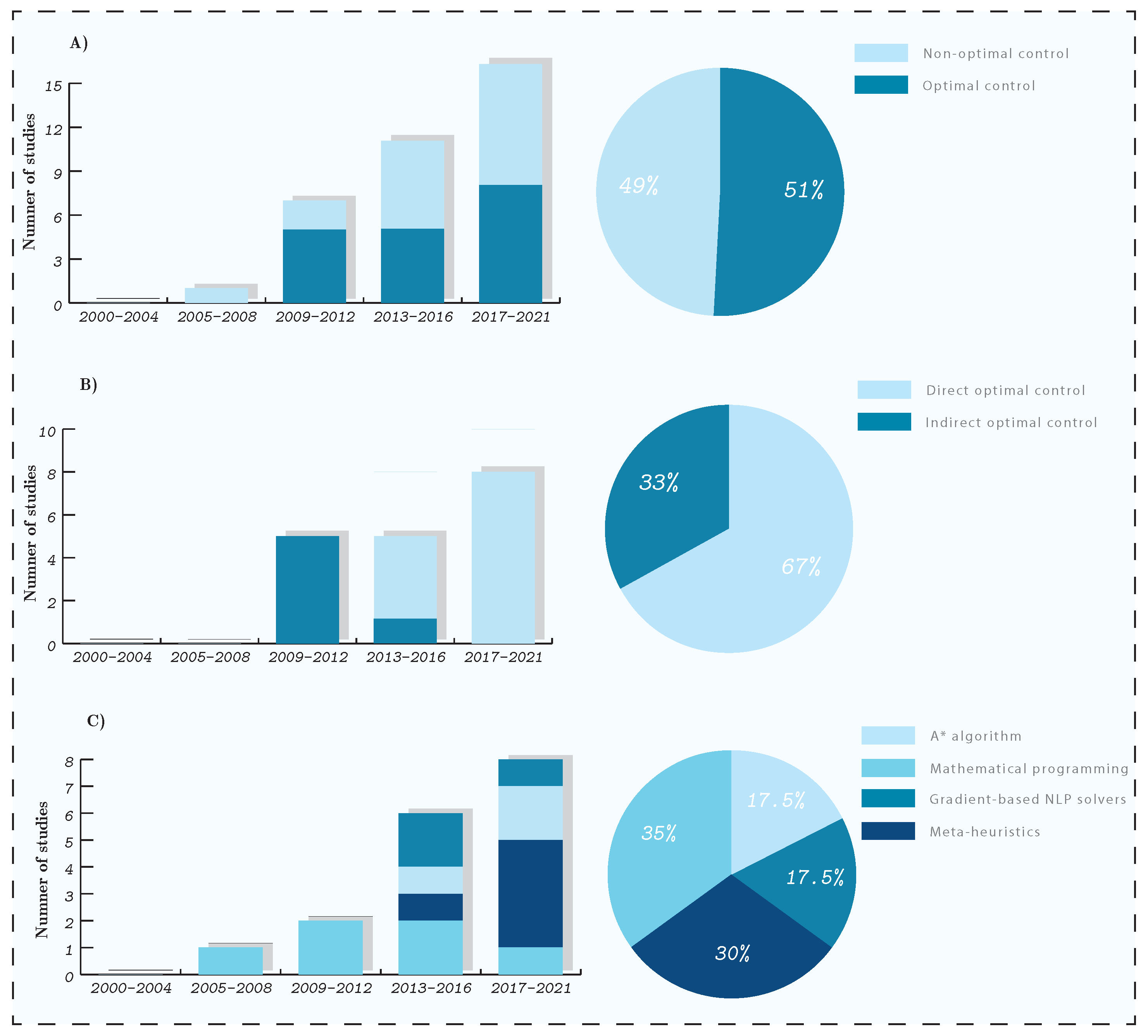
  • Although the optimal control is known as one of the most reliable approaches to solve trajectory optimization problems (at least considering the free-route concept), due to some drawbacks with the implementation, they share almost the same portion with non-optimal control methods to the total trajectory optimization-based techniques.
  • The focus has always been on conventional jet-powered aircraft.
  • The mitigation strategies using ATO techniques reviewed in this paper were mostly performed on single flights.
  • The aircraft performance, meteorological variables, and climate and cost indices were all considered deterministic in the reviewed studies.
The following section will discuss these items in detail, and a future road map is proposed.

5. Discussion and Challenges

Based on the reviewed studies, we present some challenges and scientific gaps that are crucial to be addressed in future studies in this field. In the following, the challenges will be presented in terms of required items to formulate aircraft trajectory optimization problems considering climate impact, i.e., objective function, aircraft dynamics, and solution approaches. The challenges that will be discussed regarding the objective function are referred mainly to how to model climate metrics and how to consider and quantify the associated uncertainties in the modeled metrics and the inputted meteorological variables.

5.1. Objective Function: Physical Understanding and Predictability of Aviation Climate Impacts

The determination of climate optimal trajectories relies on aircraft performance (captured by dynamic model), physical and operational constraints, and the climate impacts included in the objective function. In this respect, the actual mitigation potential relies highly on the dependability of the quantified climate impacts (from the considered metric) [49,65,89]. As has been nicely pointed out in the EU-project, FlyATM4E concept paper [95], there are different types of uncertainties to understand and quantify the climate impacts associated with aviation, such as uncertainties from climate science, uncertainties in calculating engine emissions, and uncertainties in the weather forecast. Standard weather forecasts are associated with uncertainties due to the imperfect understanding of the atmosphere, modeling errors of physical parameterization, and nonlinear, sometimes chaotic, dynamics [96,97]. Uncertainties from climate science are mainly related to the current level of scientific understanding, which is still not mature [1]. According to [95], representation of atmospheric processes, estimation of RF, and selection of physical climate metrics are the main uncertainties related to climate science.
To have a reliable estimation of mitigation potential within operational strategies, these sources of uncertainty need to be identified and quantified. For instance, an approach to quantify uncertainties due to meteorological situations is to use probabilistic weather forecasting (PWF) [98]. Among different approaches, the ensemble prediction system (EPS) is known as the most promising method in PWF [97,99,100]. EPS is a numerical weather prediction approach that generates N individual forecasts. These forecasts within EPS can be obtained using different techniques. Each forecast indicates a possible realization of weather variables, and in reality, the actual weather condition is expected to lie in the predicted dispersion of weather variables obtained using ensemble members. For instance, let us consider the climate impact of ozone in the sense of aCCF. Within the EPS forecast, we are given N different forecasts for weather-related variables, e.g., temperature and geopotential in this case, yielding N different aCCFs ( i.e., aCCF O 3 , i for i = 1 , , N ), named ensemble aCCFs. This is the same for system dynamics (due to effects of temperature and wind) and other aCCFs.
The sources of uncertainty, if not considered in the aircraft trajectory planning, will lead to unreliable solutions. To the best of our knowledge, all the studies reviewed in this survey were performed in a deterministic manner, and the determination of robust climate optimal trajectories is missing in the literature. One of the objectives of EU-project FlyATM4E is to address the mentioned sources of uncertainty in the developed aCCFs to generate robust aCCFs (i.e., R-aCCFs), allowing robust eco-efficient flight planning (interested readers are referred to [95]).

5.2. Aircraft Dynamics and Constraints: New Models for H2 and Hybrid Vehicles

While the current and short-term aviation propulsion systems are mainly based on kerosene-driven jet engines, new entrants are expected in the medium-term. This is the case of electric propulsion, H2 driven propulsion, hybrid artifacts that may combine electric/H2 driven engines with kerosene jet, and the use of sustainable aviation fuels (SAFs). In all cases, additional studies of emissions and their impact would be needed, together with new dynamical models to capture adequately the dynamical behavior of such systems.
One of particular importance is H2-powered aircraft. According to the EU’s Horizon Europe and the EU’s Clean Aviation funding programs, hydrogen propelled aircraft are thought to play a leading role in what concerns environmentally friendly aeronautics [101]. Hydrogen can potentially overcome issues related to the low capacity (mainly specific energy) of current and forthcoming batteries technology. There are two main ways to use hydrogen as an energy provider; the first one leverages on fuel cells, devices that use the chemical energy of hydrogen (or other fuels) to cleanly and efficiently produce electricity; the second strategy would use hydrogen as propellant directly in the combustion chamber of the modified engines. In both cases, hydrogen needs to be stored in tanks. Even though hydrogen-propelled aircraft are referred to as zero-carbon aircraft, this does not mean their environmental impact is negligible: Their contribution to non- C O 2 emissions, especially when it comes to water vapor and the potential formation of linear and persistent contrails, can play an equally or even larger noxious role to the environment when compared to kerosene-engine exhausts.
Needless to say, according to this survey, the focus has always been on conventional jet-powered aircraft. The analysis and climate-oriented optimization of H2-powered aircraft trajectories is missing in the literature. More efforts in the understanding of their emissions, the associated impact, and the modeling of the equations of motion and constraints are needed (e.g., see [102] for the study on the contrail coverage of hybrid-electric aircraft). When it comes to hybrid-powered vehicles, hybrid dynamical systems may be needed [103].

5.3. Solution Approach: Development of Efficient Deterministic/Stochastic Dynamical Optimization Solvers

The optimal control is known as one of the most efficient techniques to solve dynamic optimization problems, including aircraft trajectory optimization. However, as mentioned in Section 4.4, there exist some drawbacks with the numerical OC techniques in ATO. These issues are mainly related to the computational time and local optimality with the direct method, difficulty in deriving necessary conditions of optimally for complex ATO problems and solving 2PBVP with the indirect method, and curse of dimensionality with DP.
In addition, as mentioned in Section 5.1, to have reliable aircraft trajectories, the consideration of possible sources of uncertainty is necessary. After introducing suitable quantification of uncertainties (e.g., EPS forecast for meteorological uncertainty), a stochastic dynamical optimization problem needs to be solved. Considering uncertainties in the dynamical optimization problem is challenging. One of the main issues besides suitable problem formulation is the computational time. For instance, within the ensemble weather forecast, instead of considering one realization of weather variables, the optimization is to consider N probable forecasts. Several studies in the literature have proposed robust ATO considering the ensemble weather forecast; however, not within the climate optimal routing context (e.g., [104,105,106] for non-optimal control, and [107,108,109] for optimal control approaches). Following the robust optimal control-based methods proposed in [107,108,109], the dynamical model of aircraft is expanded with the number of scenarios (due to ensemble members). In this case, the dimension of state space increases linearly. Such an approach avoids the curse of dimensionality; however, it increases the computational cost and the probability of getting stuck in local solutions.
In conclusion, aircraft trajectories are to be generated with acceptable accuracy in a computationally fast manner and robust to different sources of uncertainty. Thus, the development of robust dynamical optimization solvers (mainly optimal control approach) that can satisfy these objectives is beneficial. Formulating the dynamical optimization problem to be implementable on the graphics processing unit (GPU) in a parallel manner would be efficient from the computational time perspective. For instance, in [110], by leveraging the computational power on GPU, the robust 4D trajectory in the structured airspace was optimized in seconds considering 32 ensemble members.

5.4. Network-Scale Climate Optimal Trajectories

The operational mitigation strategies using ATO techniques reviewed in this paper were mostly performed on single flights. Though some studies have run simulations with hundreds or thousands of flights, each of those flights has been tackled independently, without the consideration of interactions and network effects. Thus, the analysis of the climatic impact at the network scale is simply non-existent.
Climatic effects have not been considered as a factor to limit the capacity of the ATM system (e.g., as it is done in some European cities to limit road transportation), nor incorporated in any of the network-wide modeling and solution approaches presented in the literature. Indeed, these approaches require considering large-scale airspaces and thousands of flights, including their interactions (propagation of uncertainties at the network level and models to consider resilience). In such scenarios, the problem becomes cumbersome and very difficult to solve using classical optimization techniques.
Identifying climatic hotspots and incorporating them into network-wide models and solution approaches for problems related to, e.g., demand and capacity balancing, network complexity, and resiliency, are open scientific gaps.

6. Conclusions

This paper surveyed the recent operational techniques proposed in the literature to mitigate the climate impacts of non- C O 2 emissions. These studies were analyzed and classified mainly based on the used climate metrics and the employed operational approaches. It was concluded that the mitigation potential of aviation climate impact using operational strategies is promising. In addition, the current trend is towards trajectory optimization techniques since they can generate more efficient trajectories in the sense of mitigation potential. Moreover, some scientific gaps were identified: (1) the focus of trajectory optimization has always been on conventional jet-powered aircraft, (2) the consideration of climatic impact at the network scale is non-existent in the literature, and (3) no recent study has considered robustness with respect to the uncertainties associated with aircraft behavior, climate metrics, and meteorological conditions. Based on the identified gaps, the following future directions of research in this field were proposed:
  • Physical understanding and predictability of aviation climate impacts, particularly understanding and quantifying the uncertainties associated with climate science and meteorological forecast.
  • Better understanding of H2- and hybrid-powered aircraft emissions, the associated climate impacts, and the modeling of the equations of motion.
  • Developing high-performance dynamical optimization solvers to generate robust eco-efficient trajectories with acceptable accuracy in a computationally fast manner.
  • Identifying climatic hotspots and incorporating them into network-wide models and solution approaches for problems related to, e.g., demand and capacity balancing, network complexity, and resiliency.

Author Contributions

Conceptualization, A.S. and M.S.; writing—original draft, A.S. and M.S.; writing—review and editing, A.S., M.S., D.G.-A., S.M., V.G., S.D., S.B., H.Y., F.L., B.L., M.M.M., F.Y. and F.C.; project coordinator, S.M.; funding acquisition, S.M. All authors have read and agreed to the published version of the manuscript.

Funding

This research was carried out as a part of the project EU-project FlyATM4E. FlyATM4E has received funding from the SESAR Joint Undertaking under the European Union’s Horizon 2020 research and innovation programme under grant agreement No 891317. The JU receives support from the European Union’s Horizon 2020 research and innovation programme and the SESAR JU members other than the Union.

Data Availability Statement

Not applicable.

Conflicts of Interest

The authors declare no conflict of interest.

Abbreviations

    The following abbreviations are used in this manuscript:
ATOAircraft trajectory optimization
ATMAir traffic management
OCOptimal control
TOTrajectory optimization
NTONon-trajectory optimization
CSRClimate sensitive region
PCFAPersistent contrail formation areas
ISSRIce-supersaturated
SACSchmidt–Appleman criteria
CCFClimate change function
aCCFAlgorithmic climate change function
eCCFEmission-based climate change function
GWPGlobal warming potential
GTPGlobal temperature change potential
AGTPAbsolute global temperature potential
ATRAverage temperature response
RFRadiative forcing
PMPPontryagin’s minimum principle
HJBHamilton–Jacobi–Bellman
SOCSimple operating cost
COCCash operating cost
DOCDirect operating cost
NLPNonlinear programming
2PBVPTwo-point boundary value problems
DAEDifferential algebraic equations
FACETFuture air traffic management concepts evaluation tool
BFFM2Boeing fuel flow method 2
SQPSuccessive quadratic programming
AEDTAviation environmental design tool
FAAFederal aviation administration
MIPMixed-integer programming
MILPMixed-integer linear programming
MIQPMixed-integer quadratic programming
BIPBinary integer programming
TOMATOToolchain for multicriteria aircraft trajectory optimization
MOTOMulti-objective trajectory optimization
GAGenetic algorithm
EMACECHAM/MESSy atmospheric chemistry
TOMTrajectory optimization module
IPTInterior-point
RAMSAir traffic control mathematical simulator

Appendix A. Optimal Control Methodologies

Different optimal control methods employed in ATO are briefly presented in the following.

Appendix A.1. Pontryagin’s Minimum Principle (PMP)

Pontryagin’s minimum principle (PMP) is an analytic optimal control approach that yields the necessary conditions of optimality using the calculus of variations theory [24]. Let us consider a general dynamical optimization problem with the following Bolza form of performance index
J ( t 0 , t f , x , u ) = M t f , x ( t f ) + t 0 t f L t , x ( t ) , u ( t ) d t
and the state-space representation of the system dynamics and boundary constraints respectively as:
x ˙ ( t ) = f t , x ( t ) , u ( t ) , x ( t 0 ) = x 0 Ψ t 0 , x ( t 0 ) , t f , x ( t f ) = 0
Then, define the Hamiltonian
H ( x , u , λ , t ) : = L ( t , x , u ) + λ T ( t ) f ( t , x , u )
where λ ( t ) : R R n x is called the vector of costates. The necessary conditions for the trajectory x o to minimize the cost functional Equation (A1) while satisfying system dynamics and boundary constraints are listed as follows:
  • Euler–Lagrange equations:
    d x * d t = H λ , d λ * d t = H x
  • Transversality conditions:
    λ ( t f ) = M x + l T Ψ x t = t f
    where l R n ψ is called Lagrange multipliers.
These conditions represent the necessary conditions of optimality for the simplest problem, in which the final time is fixed, and no equality and inequality constraints are considered. For more complex problems, additional conditions are required [24]. For instance, for free final time problem we have
M t + H t = t f = 0 .
As can be seen, the differential equations characterized the necessary optimality conditions define 2PBVP. For most cases, it is not trivial to solve the resulting 2PBVP problem analytically, and usually, numerical approaches called indirect optimal control are employed.

Numerical Approach (Indirect Optimal Control)

The necessary conditions of optimality obtained from the PMP approach are solved numerically using the indirect optimal control approach. It is called indirect since we first optimize by deriving the conditions for optimality, then discretize the resulting 2PBVP to be employed by numerical solvers such as single shooting [111], and multiple shooting [112] algorithms.
Despite providing sufficient conditions for optimality, as can be seen from the formulations, non-trivial calculations are needed to derive the necessary conditions of optimality, and the derived conditions are not generic, in which, with any changes in system dynamics, constraints, or cost functional, these equations are to be calculated from the beginning. An initial guess for co-states not having physical interpretations is required here in addition to other parameters within the numerical solvers [113].

Appendix A.2. Hamilton-Jacobi-Bellman (HJB)

The HJB equation provides sufficient conditions of optimality represented with partial differential equations (PDE). Let consider the state-space representation of system dynamics and cost functional as Equations (A1) and (A2), respectively. The optimal control policy in the form of u o ( t ) = k t , x ( t ) is the solution of the following minimization problem
u o ( t ) = arg min u L ( t , x , u ) + V x T ( t , x ) · f ( t , x , u )
where V ( · ) is called value function defined as the minimum value of the cost functional, i.e.,
V ( t , x ) = min u M t f , x ( t f ) + t 0 t f L t , x ( t ) , u ( t ) d t
which must satisfy the following PDE, called HJB equation
V t ( t , x ) = min u L ( t , x , u ) + V x T ( t , x ) · f ( t , x , u )
with the boundary condition V ( t f , x ( t f ) ) = M t f , x ( t f ) . An analytic solution to the HJB equation is very difficult due to the resulting partial differential equations, and only for some simple cases such as quadratic performance index with linear system dynamics called linear quadratic optimization problem, the analytic solutions have been developed [26].

Numerical Approach (Dynamic Programming)

If one discretizes the continuous dynamical optimization problem, the following recurrence form of the HJB equation can be employed:
V k ( x n k ) = min u n k L ^ ( x n k , u n k ) + V k 1 ( f ^ ( x n k , u n k )
which is known as the Bellman equation. In Equation (A10), n is the number of steps, k is the k-th step, and ( · ^ ) denotes the discrete approximation. The main drawback associated with the discrete HJB (i.e., DP) is the computational cost which is high for systems with more than a few states. In other words, it causes the “curse of dimensionality”, which refers to an exponential increase in the required computational resources with the dimension of the dynamical system.
Despite the high computational efforts needed to calculate the optimal solution, this method has some advantages, such as resulting in global solutions, providing a closed-loop policy, and the ability to extend the results to stochastic problems. Moreover, some techniques approximating different components of the original dynamic programming problem have been proposed to enhance the computational cost. These methods are called approximate (or adaptive) dynamic programming (interested readers are referred to two valuable books by Bertsekas [114] and Powell [115]).

Appendix A.3. Direct Optimal Control

The direct optimal control approach attempts to directly solve the optimal control problem by discretization and conversion to the NLP problem. Unlike the indirect approach, which first optimizes, then discretizes, the direct methods first discretize then optimize. Mathematically, a dynamical optimization problem with the cost functional, system dynamics, equality and inequality path, and boundary constraints after suitable transcription is converted to an NLP problem as the following form [28]
min Λ J d ( Λ )
s . t Φ i ( Λ ) = 0 i = 1 , , n ϕ
Ψ i ( Λ ) 0 i = 1 , , n ψ
where Λ R n Λ is the vector of NLP (or decision) variables and Equations (A12) and (A13) represent the equality and inequality constraints. In this case, the optimal solution to the original optimal control problem is achieved from solving the obtained NLP problem.
The direct methods mainly differ in how they convert each aspect of the dynamic optimization problem to the discrete form. One may classify the direct approach as direct shooting and direct collocation methods [27,28]. Within the transcription using the direct shooting approach, the control variables are discretized and considered as decision variables. In contrast, both control and state variables are discretized and taken as NLP variables in direct collocation methods.
The resulting NLP problem can be solved using different techniques such as interior-point and SQP [27,28] as classic (or gradient-based) NLP solvers or meta-heuristic methods. Besides, to solve the NLP problem, several powerful packages, including SNOPT [116], fmincon function in MATLAB, KNITRO [117], DONLP2 [118], GAMS [119], and IPOPT [120] exist. After solving the NLP problem, an optimal decision vector will be obtained ( Λ o ), which is to be interpolated to be reconverted back to the continuous domain.
From the brief presentation of the direct optimal control, one can conclude that this approach is more efficient in dealing with more complex dynamical optimization problems since it can efficiently consider nonlinearity and constraints by discretizing the original problem and determining optimal solution through the NLP problem. In spite of such valuable advantages, it is noteworthy that this approach, in general, is not suitable for real-time optimizations (due to the computational time) and closed-loop controlling schemes. Moreover, local optimality is another limitation of the direct approach in solving complex problems [27,28].

References

  1. Lee, D.S.; Fahey, D.; Skowron, A.; Allen, M.; Burkhardt, U.; Chen, Q.; Doherty, S.; Freeman, S.; Forster, P.; Fuglestvedt, J.; et al. The contribution of global aviation to anthropogenic climate forcing for 2000 to 2018. Atmos. Environ. 2021, 244, 117834. [Google Scholar] [CrossRef]
  2. Forecast, Global Market. Future Journeys 2013; Technical Report; Airbus: Leiden, The Netherlands, 2013. [Google Scholar]
  3. Lee, D.S.; Fahey, D.W.; Forster, P.M.; Newton, P.J.; Wit, R.C.; Lim, L.L.; Owen, B.; Sausen, R. Aviation and global climate change in the 21st century. Atmos. Environ. 2009, 43, 3520–3537. [Google Scholar] [CrossRef] [Green Version]
  4. Lee, D.S.; Pitari, G.; Grewe, V.; Gierens, K.; Penner, J.E.; Petzold, A.; Prather, M.; Schumann, U.; Bais, A.; Berntsen, T.; et al. Transport impacts on atmosphere and climate: Aviation. Atmos. Environ. 2010, 44, 4678–4734. [Google Scholar] [CrossRef] [Green Version]
  5. Bolić, T.; Ravenhill, P. SESAR: The Past, Present, and Future of European Air Traffic Management Research. Engineering 2021, 7, 448–451. [Google Scholar] [CrossRef]
  6. Gnadt, A.R.; Speth, R.L.; Sabnis, J.S.; Barrett, S.R. Technical and environmental assessment of all-electric 180-passenger commercial aircraft. Prog. Aerosp. Sci. 2019, 105, 1–30. [Google Scholar] [CrossRef] [Green Version]
  7. Ribeiro, J.; Afonso, F.; Ribeiro, I.; Ferreira, B.; Policarpo, H.; Peças, P.; Lau, F. Environmental assessment of hybrid-electric propulsion in conceptual aircraft design. J. Clean. Prod. 2020, 247, 119477. [Google Scholar] [CrossRef]
  8. Staples, M.D.; Malina, R.; Suresh, P.; Hileman, J.I.; Barrett, S.R. Aviation CO2 emissions reductions from the use of alternative jet fuels. Energy Policy 2018, 114, 342–354. [Google Scholar] [CrossRef]
  9. Stratton, R.W.; Wolfe, P.J.; Hileman, J.I. Impact of aviation non-CO2 combustion effects on the environmental feasibility of alternative jet fuels. Environ. Sci. Technol. 2011, 45, 10736–10743. [Google Scholar] [CrossRef]
  10. Delahaye, D.; Puechmorel, S.; Tsiotras, P.; Féron, E. Mathematical models for aircraft trajectory design: A survey. In Air Traffic Management and Systems; Springer: Berlin/Heidelberg, Germany, 2014; pp. 205–247. [Google Scholar]
  11. Gardi, A.; Sabatini, R.; Ramasamy, S. Multi-objective optimisation of aircraft flight trajectories in the ATM and avionics context. Prog. Aerosp. Sci. 2016, 83, 1–36. [Google Scholar] [CrossRef]
  12. Mannstein, H.; Spichtinger, P.; Gierens, K. A note on how to avoid contrail cirrus. Transp. Res. Part D Transp. Environ. 2005, 10, 421–426. [Google Scholar] [CrossRef]
  13. Zou, B.; Buxi, G.S.; Hansen, M. Optimal 4-D aircraft trajectories in a contrail-sensitive environment. Netw. Spat. Econ. 2016, 16, 415–446. [Google Scholar] [CrossRef]
  14. Hammad, A.W.; Rey, D.; Bu-Qammaz, A.; Grzybowska, H.; Akbarnezhad, A. Mathematical optimization in enhancing the sustainability of aircraft trajectory: A review. Int. J. Sustain. Transp. 2020, 14, 413–436. [Google Scholar] [CrossRef]
  15. Matthes, S.; Schumann, U.; Grewe, V.; Frömming, C.; Dahlmann, K.; Koch, A.; Mannstein, H. Climate optimized air transport. In Atmospheric Physics; Springer: Berlin/Heidelberg, Germany, 2012; pp. 727–746. [Google Scholar]
  16. Niklaß, M.; Lührs, B.; Grewe, V.; Dahlmann, K.; Luchkova, T.; Linke, F.; Gollnick, V. Potential to reduce the climate impact of aviation by climate restricted airspaces. Transp. Policy 2019, 83, 102–110. [Google Scholar] [CrossRef]
  17. Williams, V.; Noland, R.B.; Toumi, R. Air transport cruise altitude restrictions to minimize contrail formation. Clim. Policy 2003, 3, 207–219. [Google Scholar] [CrossRef]
  18. Williams, V.; Noland, R.B. Variability of contrail formation conditions and the implications for policies to reduce the climate impacts of aviation. Transp. Res. Part D Transp. Environ. 2005, 10, 269–280. [Google Scholar] [CrossRef]
  19. Campbell, S.; Neogi, N.; Bragg, M. An operational strategy for persistent contrail mitigation. In Proceedings of the 9th AIAA Aviation Technology, Integration, and Operations Conference (ATIO) and Aircraft Noise and Emissions Reduction Symposium (ANERS), Hilton Head, SC, USA, 21–23 September 2009; p. 6983. [Google Scholar]
  20. Sridhar, B.; Ng, H.K.; Chen, N.Y. Aircraft trajectory optimization and contrails avoidance in the presence of winds. J. Guid. Control Dyn. 2011, 34, 1577–1584. [Google Scholar] [CrossRef]
  21. Gierens, K.M.; Lim, L.; Eleftheratos, K. A review of various strategies for contrail avoidance. Open Atmos. Sci. J. 2008, 2, 1–7. [Google Scholar] [CrossRef] [Green Version]
  22. Chai, R.; Savvaris, A.; Tsourdos, A.; Chai, S.; Xia, Y. A review of optimization techniques in spacecraft flight trajectory design. Prog. Aerosp. Sci. 2019, 109, 100543. [Google Scholar] [CrossRef]
  23. Morante, D.; Sanjurjo Rivo, M.; Soler, M. A Survey on Low-Thrust Trajectory Optimization Approaches. Aerospace 2021, 8, 88. [Google Scholar] [CrossRef]
  24. Kirk, D.E. Optimal Control Theory: An Introduction; Courier Corporation: Chelmsford, MA, USA, 2004. [Google Scholar]
  25. Zhou, K.; Doyle, J.; Glover, K. Robust and Optimal Control; Prentice Hall: Hoboken, NJ, USA, 1996. [Google Scholar]
  26. Lewis, F.L.; Vrabie, D.; Syrmos, V.L. Optimal Control; John Wiley & Sons: Hoboken, NJ, USA, 2012. [Google Scholar]
  27. Chachuat, B. Nonlinear and Dynamic Optimization: From Theory to Practice; Technical Report; Laboratoire d’Automatique, École Polytechnique Fédérale de Lausanne: Lausanne, Switzerland, 2007. [Google Scholar]
  28. Betts, J.T. Practical Methods for Optimal Control and Estimation Using Nonlinear Programming, 2nd ed.; Advances in Design and Control; SIAM: Philadelphia, PA, USA, 2010. [Google Scholar]
  29. Yamashita, H.; Yin, F.; Grewe, V.; Jöckel, P.; Matthes, S.; Kern, B.; Dahlmann, K.; Frömming, C. Newly developed aircraft routing options for air traffic simulation in the chemistry–climate model EMAC 2.53: AirTraf 2.0. Geosci. Model Dev. 2020, 13, 4869–4890. [Google Scholar] [CrossRef]
  30. Förster, S.; Rosenow, J.; Lindner, M.; Fricke, H. A toolchain for optimizing trajectories under real weather conditions and realistic flight performance. In Proceedings of the Greener Aviation Conference, Brussels, Belgium, 13–17 October 2016. [Google Scholar]
  31. Yamashita, H.; Yin, F.; Grewe, V.; Jöckel, P.; Matthes, S.; Kern, B.; Dahlmann, K.; Frömming, C. Analysis of aircraft routing strategies for north atlantic flights by using AirTraf 2.0. Aerospace 2021, 8, 33. [Google Scholar] [CrossRef]
  32. Rosenow, J.; Förster, S.; Lindner, M.; Fricke, H. Multicriteria-Optimized Trajectories Impacting Today’s Air Traffic Density, Efficiency, and Environmental Compatibility. J. Air Transp. 2019, 27, 8–15. [Google Scholar] [CrossRef]
  33. Dallara, E.S.; Kroo, I.M.; Waitz, I.A. Metric for comparing lifetime average climate impact of aircraft. AIAA J. 2011, 49, 1600–1613. [Google Scholar] [CrossRef]
  34. Fuglestvedt, J.S.; Shine, K.P.; Berntsen, T.; Cook, J.; Lee, D.; Stenke, A.; Skeie, R.B.; Velders, G.; Waitz, I. Transport impacts on atmosphere and climate: Metrics. Atmos. Environ. 2010, 44, 4648–4677. [Google Scholar] [CrossRef] [Green Version]
  35. Shine, K.P.; Fuglestvedt, J.S.; Hailemariam, K.; Stuber, N. Alternatives to the global warming potential for comparing climate impacts of emissions of greenhouse gases. Clim. Chang. 2005, 68, 281–302. [Google Scholar] [CrossRef] [Green Version]
  36. Celis, C.; Sethi, V.; Zammit-Mangion, D.; Singh, R.; Pilidis, P. Theoretical optimal trajectories for reducing the environmental impact of commercial aircraft operations. J. Aerosp. Technol. Manag. 2014, 6, 29–42. [Google Scholar] [CrossRef]
  37. Jelinek, F. The Advanced Emission Model (AEM3)-Validation Report. Ratio 2004, 306, 1–13. [Google Scholar]
  38. DuBois, D.; Paynter, G.C. “Fuel Flow Method2” for Estimating Aircraft Emissions. SAE Trans. 2006, 115, 1–14. [Google Scholar]
  39. Soler, M.; Zou, B.; Hansen, M. Flight trajectory design in the presence of contrails: Application of a multiphase mixed-integer optimal control approach. Transp. Res. Part C Emerg. Technol. 2014, 48, 172–194. [Google Scholar] [CrossRef]
  40. Sridhar, B.; Chen, N.Y.; Ng, H.K.; Linke, F. Design of aircraft trajectories based on trade-offs between emission. In Proceedings of the 9th USA/Europe Air Traffic Management Research and Development Seminar (ATM2011), Berlin, Germany, 14–17 June 2011. [Google Scholar]
  41. Reutter, P.; Neis, P.; Rohs, S.; Sauvage, B. Ice supersaturated regions: Properties and validation of ERA-Interim reanalysis with IAGOS in situ water vapour measurements. Atmos. Chem. Phys. 2020, 20, 787–804. [Google Scholar] [CrossRef] [Green Version]
  42. Schumann, U. On conditions for contrail formation from aircraft exhausts. Meteorol. Z. 1996, 5, 4–23. [Google Scholar] [CrossRef]
  43. Schmidt, E. Die Entstehung von Eisnebel aus den Auspuffgasen von Flugmotoren; Verlag R. Oldenbourg: München, Germany, 1941. [Google Scholar]
  44. Appleman, H. The formation of exhaust condensation trails by jet aircraft. Bull. Am. Meteorol. Soc. 1953, 34, 14–20. [Google Scholar] [CrossRef] [Green Version]
  45. Burkhardt, U.; Kärcher, B.; Ponater, M.; Gierens, K.; Gettelman, A. Contrail cirrus supporting areas in model and observations. Geophys. Res. Lett. 2008, 35, 1–5. [Google Scholar] [CrossRef] [Green Version]
  46. Yin, F.; Grewe, V.; Frömming, C.; Yamashita, H. Impact on flight trajectory characteristics when avoiding the formation of persistent contrails for transatlantic flights. Transp. Res. Part D Transp. Environ. 2018, 65, 466–484. [Google Scholar] [CrossRef]
  47. Lim, Y.; Gardi, A.; Marino, M.; Sabatini, R. Modelling and evaluation of persistent contrail formation regions for offline and online strategic flight trajectory planning. In Sustainable Aviation; Springer: Berlin/Heidelberg, Germany, 2016; pp. 243–277. [Google Scholar]
  48. Lim, Y.; Gardi, A.; Sabatini, R. Optimal aircraft trajectories to minimize the radiative impact of contrails and CO2. Energy Procedia 2017, 110, 446–452. [Google Scholar] [CrossRef]
  49. Grewe, V.; Frömming, C.; Matthes, S.; Brinkop, S.; Ponater, M.; Dietmüller, S.; Jöckel, P.; Garny, H.; Tsati, E.; Dahlmann, K.; et al. Aircraft routing with minimal climate impact: The REACT4C climate cost function modelling approach (V1. 0). Geosci. Model Dev. 2014, 7, 175–201. [Google Scholar] [CrossRef] [Green Version]
  50. Lee, D.; Arrowsmith, S.; Skowron, A.; Owen, B.; Sausen, R.; Boucher, O.; Faber, J.; Marianne, L.; Fuglestvedt, J.; van Wijngaarden, L. Updated Analysis of the Non-CO2 Climate Impacts of Aviation and Potential Policy Measures Pursuant to EU Emissions Trading System Directive Article 30(4). 2020. Available online: https://www.easa.europa.eu/document-library/research-reports/report-commission-european-parliament-and-council (accessed on 8 February 2022).
  51. Ng, H.K.; Sridhar, B.; Grabbe, S.; Chen, N. Cross-polar aircraft trajectory optimization and the potential climate impact. In Proceedings of the 2011 IEEE/AIAA 30th Digital Avionics Systems Conference, Seattle, WA, USA, 21 July 2011. [Google Scholar]
  52. González Arribas, D. Robust Aircraft Trajectory Optimization under Meteorological Uncertainty. Ph.D. Dissertation, Universidad Carlos III de Madrid, Madrid, Spain, July 2019. [Google Scholar]
  53. Kirkpatrick, S.; Gelatt, C.D.; Vecchi, M.P. Optimization by simulated annealing. Science 1983, 220, 671–680. [Google Scholar] [CrossRef]
  54. Deb, K.; Agrawal, S.; Pratap, A.; Meyarivan, T. A fast elitist non-dominated sorting genetic algorithm for multi-objective optimization: NSGA-II. In Proceedings of the International Conference on Parallel Problem Solving from Nature, Paris, France, 18–20 September 2000; Springer: Berlin/Heidelberg, Germany, 2000; pp. 849–858. [Google Scholar]
  55. Mladenović, N.; Hansen, P. Variable neighborhood search. Comput. Oper. Res. 1997, 24, 1097–1100. [Google Scholar] [CrossRef]
  56. Shi, Y.; Eberhart, R. A modified particle swarm optimizer. In Proceedings of the 1998 IEEE International Conference on Evolutionary Computation Proceedings, IEEE World Congress on Computational Intelligence (Cat. No. 98TH8360), Anchorage, AK, USA, 4–9 May 1998; pp. 69–73. [Google Scholar]
  57. Kennedy, J.; Eberhart, R. Particle swarm optimization. In Proceedings of the ICNN’95-International Conference on Neural Networks, IEEE, Perth, Australia, 27 November–1 December 1995; Volume 4, pp. 1942–1948. [Google Scholar]
  58. Myhre, G.; Stordal, F. On the tradeoff of the solar and thermal infrared radiative impact of contrails. Geophys. Res. Lett. 2001, 28, 3119–3122. [Google Scholar] [CrossRef]
  59. Williams, V.; Noland, R.B.; Toumi, R. Reducing the climate change impacts of aviation by restricting cruise altitudes. Transp. Res. Part D Transp. Environ. 2002, 7, 451–464. [Google Scholar] [CrossRef]
  60. Sausen, R.; Gierens, K.; Ponater, M.; Schumann, U. A diagnostic study of the global distribution of contrails part I: Present day climate ast. Theor. Appl. Climatol. 1998, 61, 127–141. [Google Scholar] [CrossRef] [Green Version]
  61. Fichter, C.; Marquart, S.; Sausen, R.; Lee, D.S. The impact of cruise altitude on contrails and related radiative forcing. Meteorol. Z. 2005, 14, 563–572. [Google Scholar] [CrossRef] [Green Version]
  62. Klima, K. Assessment of a Global Contrail Modeling Method and Operational Strategies for Contrail Mitigation. Ph.D. Thesis, Massachusetts Institute of Technology, Cambridge, MA, USA, 2005. [Google Scholar]
  63. Chen, N.Y.; Sridhar, B.; Ng, H.K. Tradeoff between contrail reduction and emissions in United States national airspace. J. Aircr. 2012, 49, 1367–1375. [Google Scholar] [CrossRef]
  64. Chen, N.Y.; Sridhar, B.; Ng, H.; Li, J. Evaluating tradeoff between environmental impact and operational costs for enroute air traffic. In Proceedings of the AIAA Guidance, Navigation, and Control Conference, National Harbor, MD, USA, 13–17 January 2014; p. 1464. [Google Scholar]
  65. Grewe, V.; Champougny, T.; Matthes, S.; Frömming, C.; Brinkop, S.; Søvde, O.A.; Irvine, E.A.; Halscheidt, L. Reduction of the air traffic’s contribution to climate change: A REACT4C case study. Atmos. Environ. 2014, 94, 616–625. [Google Scholar] [CrossRef] [Green Version]
  66. Jöckel, P.; Kerkweg, A.; Pozzer, A.; Sander, R.; Tost, H.; Riede, H.; Baumgaertner, A.; Gromov, S.; Kern, B. Development cycle 2 of the modular earth submodel system (MESSy2). Geosci. Model Dev. 2010, 3, 717–752. [Google Scholar] [CrossRef] [Green Version]
  67. Brenninkmeijer, C.A.; Cai, D.S. Earth System Chemistry integrated Modelling (ESCiMo) with the Modular Earth Submodel System (MESSy) version 2.51. Geosci. Model Dev. 2016, 9, 1153. [Google Scholar]
  68. Frömming, C.; Grewe, V.; Jöckel, P.; Brinkop, S.; Dietmüller, S.; Garny, H.; Ponater, M.; Tsati, E.; Matthes, S. Climate cost functions as a basis for climate optimized flight trajectories. Air Traffic Semin. 2013, 239, 1–9. [Google Scholar]
  69. Irvine, E.A.; Hoskins, B.J.; Shine, K.P.; Lunnon, R.W.; Froemming, C. Characterizing North Atlantic weather patterns for climate-optimal aircraft routing. Meteorol. Appl. 2013, 20, 80–93. [Google Scholar] [CrossRef] [Green Version]
  70. Grewe, V.; Matthes, S.; Frömming, C.; Brinkop, S.; Jöckel, P.; Gierens, K.; Champougny, T.; Fuglestvedt, J.; Haslerud, A.; Irvine, E.; et al. Feasibility of climate-optimized air traffic routing for trans-Atlantic flights. Environ. Res. Lett. 2017, 12, 034003. [Google Scholar] [CrossRef]
  71. Campbell, S.; Neogi, N.; Bragg, M. An optimal strategy for persistent contrail avoidance. In Proceedings of the AIAA Guidance, Navigation and Control Conference and Exhibit, Monterey, CA, USA, 19 August 2008; p. 6515. [Google Scholar]
  72. Wei, P.; Sridhar, B.; Chen, N.; Sun, D. A Linear Programming Approach to the Development of Contrail Reduction Strategies Satisfying Operationally Feasible Constraints. In Proceedings of the AIAA Guidance, Navigation, and Control Conference, Garden Grove, CA, USA, 13–16 August 2012; p. 4754. [Google Scholar]
  73. Campbell, S.E.; Bragg, M.B.; Neogi, N.A. Fuel-optimal trajectory generation for persistent contrail mitigation. J. Guid. Control Dyn. 2013, 36, 1741–1750. [Google Scholar] [CrossRef]
  74. Lim, Y.; Gardi, A.; Sabatini, R. Modelling and evaluation of aircraft contrails for 4-dimensional trajectory optimisation. SAE Int. J. Aerosp. 2015, 8, 248–259. [Google Scholar] [CrossRef]
  75. Rosenow, J.; Förster, S.; Lindner, M.; Fricke, H. Impact of multi-critica optimized trajectories on European air traffic density, efficiency and the environment. In Proceedings of the Twelfth USA/Europe Air Traffic Management Research and Development Seminar, Seattle, WA, USA, 27–30 June 2017; pp. 26–30. [Google Scholar]
  76. Yin, F.; Grewe, V.; van Manen, J.; Matthes, S.; Yamashita, H.; Linke, F.; Lührs, B. Verification of the ozone algorithmic climate change functions for predicting the short-term NOx effects from aviation en-route. In Proceedings of the International Conference on Research in Air Transportation (ICRAT), Barcelona, Spain, 26–29 June 2018. [Google Scholar]
  77. Yamashita, H.; Grewe, V.; Jöckel, P.; Linke, F.; Schaefer, M.; Sasaki, D. Air traffic simulation in chemistry-climate model EMAC 2.41: AirTraf 1.0. Geosci. Model Dev. 2016, 9, 3363–3392. [Google Scholar] [CrossRef] [Green Version]
  78. Yamashita, H.; Grewe, V.; Jöckel, P.; Linke, F.; Schaefer, M.; Sasaki, D. Towards climate optimized flight trajectories in a climate model: AirTraf. In Proceedings of the Eleventh USA/Europe Air Traffic Management Research and Development Seminar (ATM2015), Lisbon, Portugal, 23–26 June 2015; pp. 23–26. [Google Scholar]
  79. Sasaki, D.; Obayashi, S.; Nakahashi, K. Navier-Stokes optimization of supersonic wings with four objectives using evolutionary algorithm. J. Aircr. 2002, 39, 621–629. [Google Scholar] [CrossRef]
  80. Sasaki, D.; Obayashi, S. Efficient search for trade-offs by adaptive range multi-objective genetic algorithms. J. Aerosp. Comput. Inform. Commun. 2005, 2, 44–64. [Google Scholar] [CrossRef] [Green Version]
  81. Sasaki, D.; Obayashi, S. Development of Efficient Multi-Objective Evolutionary Algorithms: ARMOGAs (Adaptive Range Multi-Objective Genetic Algorithms); Institute of Fluid Science, Tohoku University: Sendai, Japan, 2004; Volume 16, pp. 11–18. [Google Scholar]
  82. Van Manen, J.; Grewe, V. Algorithmic climate change functions for the use in eco-efficient flight planning. Transp. Res. Part D Transp. Environ. 2019, 67, 388–405. [Google Scholar] [CrossRef]
  83. Rosenow, J.; Fricke, H. Flight Performance Modeling to Optimize Trajectories; Deutsche Gesellschaft für Luft-und Raumfahrt-Lilienthal-Oberth eV: Bonn, Germany, 2016. [Google Scholar]
  84. Sridhar, B.; Chen, N.; Ng, H.K. Simulation and Optimization Methods for Assessing the Impact of Aviation Operations on the Environment. In Proceedings of the 27th International Congress of the Aeronautical Sciences (ICAS2010), Nice, France, 19–24 September 2010; pp. 1–11. [Google Scholar]
  85. Lührs, B.; Linke, F.; Gollnick, V. Erweiterung eines Trajektorienrechners zur Nutzung meteorologischer Daten für die Optimierung von Flugzeugtrajektorien. In Proceedings of the Deutscher Luft- und Raumfahrtkongress (DLRK), Augsburg, Germany, 16–18 September 2014. [Google Scholar]
  86. Hartjes, S.; Hendriks, T.; Visser, D. Contrail mitigation through 3D aircraft trajectory optimization. In Proceedings of the 16th AIAA Aviation Technology, Integration, and Operations Conference, Washington, DC, USA, 13–17 June 2016; p. 3908. [Google Scholar]
  87. Lührs, B.; Niklass, M.; Froemming, C.; Grewe, V.; Gollnick, V. Cost-benefit assessment of 2D and 3D climate and weather optimized trajectories. In Proceedings of the 16th AIAA Aviation Technology, Integration, and Operations Conference, Washington, DC, USA, 13–17 June 2016; p. 3758. [Google Scholar]
  88. Niklaß, M.; Lührs, B.; Ghosh, R. A note on how to internalize aviation’s climate impact of non-CO2 effects. In Proceedings of the 2nd ECATS Conference, Athens, Greece, 7–9 November 2016; pp. 7–9. [Google Scholar]
  89. Matthes, S.; Grewe, V.; Dahlmann, K.; Frömming, C.; Irvine, E.; Lim, L.; Linke, F.; Lührs, B.; Owen, B.; Shine, K.; et al. A concept for multi-criteria environmental assessment of aircraft trajectories. Aerospace 2017, 4, 42. [Google Scholar] [CrossRef] [Green Version]
  90. Lührs, B.; Linke, F.; Matthes, S.; Grewe, V.; Yin, F. Climate impact mitigation potential of European air traffic in a weather situation with strong contrail formation. Aerospace 2021, 8, 50. [Google Scholar] [CrossRef]
  91. Matthes, S.; Lührs, B.; Dahlmann, K.; Grewe, V.; Linke, F.; Yin, F.; Klingaman, E.; Shine, K.P. Climate-optimized trajectories and robust mitigation potential: Flying ATM4E. Aerospace 2020, 7, 156. [Google Scholar] [CrossRef]
  92. Niklaß, M.; Grewe, V.; Gollnick, V.; Dahlmann, K. Concept of climate-charged airspaces: A potential policy instrument for internalizing aviation’s climate impact of non-CO2 effects. Clim. Policy 2021, 21, 1066–1085. [Google Scholar] [CrossRef]
  93. Vitali, A.; Battipede, M.; Lerro, A. Multi-Objective and Multi-Phase 4D Trajectory Optimization for Climate Mitigation-Oriented Flight Planning. Aerospace 2021, 8, 395. [Google Scholar] [CrossRef]
  94. Niklaß, M.; Gollnick, V.; Lührs, B.; Dahlmann, K.; Froemming, C.; Grewe, V.; van Manen, J. Cost-benefit assessment of climate-restricted airspaces as an interim climate mitigation option. J. Air Transp. 2017, 25, 27–38. [Google Scholar] [CrossRef]
  95. Matthes, S.; Dahlmann, K.; Dietmüller, S.; Yamashita, H.; Baumann, S.; Grewe, V.; Soler, M.; Simorgh, A.; González Arribas, D.; Linke, F.; et al. Concept for Identifying Robust Eco-Efficient Aircraft Trajectories: Methodological Concept of Climate-Optimised Aircraft Trajectories in FlyATM4E; Deutsches Zentrum für Luft- und Raumfahrt (DLR), Institut für Physik der Atmosphäre: Oberpfaffenhofen, Germany, 2022; manuscript in preparation. [Google Scholar]
  96. Bauer, P.; Thorpe, A.; Brunet, G. The quiet revolution of numerical weather prediction. Nature 2015, 525, 47–55. [Google Scholar] [CrossRef] [PubMed]
  97. WMO. Guidelines on Ensemble Prediction Systems and Forecasting; World Meteorological Organization (WMO): Geneva, Switzerland, 2012. [Google Scholar]
  98. Council, A. Enhancing weather information with probability forecasts. Bull. Am. Meteorol. Soc. 2008, 89, 1049–1053. [Google Scholar]
  99. Krishnamurti, T.N.; Kishtawal, C.; Zhang, Z.; LaRow, T.; Bachiochi, D.; Williford, E.; Gadgil, S.; Surendran, S. Multimodel ensemble forecasts for weather and seasonal climate. J. Clim. 2000, 13, 4196–4216. [Google Scholar] [CrossRef]
  100. Komma, J.; Reszler, C.; Blöschl, G.; Haiden, T. Ensemble prediction of floods–catchment non-linearity and forecast probabilities. Nat. Hazards Earth Syst. Sci. 2007, 7, 431–444. [Google Scholar] [CrossRef] [Green Version]
  101. Fuel Cells and Hydrogen Joint Undertaking. In Hydrogen-Powered Aviation: A Fact-Based Study of Hydrogen Technology, Economics, and Climate Impact by 2050; FCH JU Publications: Luxembourg, 2020.
  102. Yin, F.; Grewe, V.; Gierens, K. Impact of Hybrid-Electric Aircraft on Contrail Coverage. Aerospace 2020, 7, 147. [Google Scholar] [CrossRef]
  103. Branicky, M.S.; Borkar, V.S.; Mitter, S.K. A unified framework for hybrid control: Model and optimal control theory. IEEE Trans. Autom. Control 1998, 43, 31–45. [Google Scholar] [CrossRef] [Green Version]
  104. Franco, A.; Rivas, D.; Valenzuela, A. Optimal aircraft path planning considering wind uncertainty. In Proceedings of the European Conference for Aeronautics and Space Sciences (EUCASS), Milan, Italy, 3–6 July 2017. [Google Scholar]
  105. Franco Espín, A.; Rivas Rivas, D.; Valenzuela Romero, A. Optimal Aircraft Path Planning in a Structured Airspace Using Ensemble Weather Forecasts. In Proceedings of the 8th SESAR Innovation Days, Salzburg, Austria, 3–7 December 2018. [Google Scholar]
  106. Legrand, K.; Puechmorel, S.; Delahaye, D.; Zhu, Y. Robust aircraft optimal trajectory in the presence of wind. IEEE Aerosp. Electron. Syst. Mag. 2018, 33, 30–38. [Google Scholar] [CrossRef]
  107. González-Arribas, D.; Soler, M.; Sanjurjo-Rivo, M. Robust aircraft trajectory planning under wind uncertainty using optimal control. J. Guid. Control Dyn. 2018, 41, 673–688. [Google Scholar] [CrossRef] [Green Version]
  108. González-Arribas, D.; Soler, M.; Sanjurjo-Rivo, M.; García-Heras, J.; Sacher, D.; Gelhardt, U.; Lang, J.; Hauf, T.; Simarro, J. Robust optimal trajectory planning under uncertain winds and convective risk. In ENRI International Workshop on ATM/CNS; Springer: Berlin/Heidelberg, Germany, 2017; pp. 82–103. [Google Scholar]
  109. Kamo, S.; Rosenow, J.; Fricke, H. CDO Sensitivity Analysis for Robust Trajectory Planning under Uncertain Weather Prediction. In Proceedings of the 2020 AIAA/IEEE 39th Digital Avionics Systems Conference (DASC), San Antonio, TX, USA, 11–15 October 2020; pp. 1–10. [Google Scholar] [CrossRef]
  110. González Arribas, D.; Andrés-Enderiz, E.; Soler, M.; Jardines, A.; García-Heras, J. Probabilistic 4D Flight Planning in Structured Airspaces through Parallelized Simulation on GPUs. In Proceedings of the 9th International Conference for Research in Air Transportation (ICRAT), Online, 15 September 2020. [Google Scholar]
  111. Von Stryk, O.; Bulirsch, R. Direct and indirect methods for trajectory optimization. Ann. Oper. Res. 1992, 37, 357–373. [Google Scholar] [CrossRef]
  112. Carraro, T.; Geiger, M.; Rannacher, R. Indirect multiple shooting for nonlinear parabolic optimal control problems with control constraints. SIAM J. Sci. Comput. 2014, 36, A452–A481. [Google Scholar] [CrossRef] [Green Version]
  113. Fidanova, S.; Ditzinger. Recent Advances in Computational Optimization; Springer: Berlin/Heidelberg, Germany, 2013. [Google Scholar]
  114. Bertsekas, D. Reinforcement Learning and Optimal Control; Athena Scientific: Belmont, MA, USA, 2019. [Google Scholar]
  115. Powell, W.B. Approximate Dynamic Programming: Solving the Curses of Dimensionality; John Wiley & Sons: Hoboken, NJ, USA, 2007; Volume 703. [Google Scholar]
  116. Gill, P.E.; Murray, W.; Saunders, M.A. SNOPT: An SQP algorithm for large-scale constrained optimization. SIAM Rev. 2005, 47, 99–131. [Google Scholar] [CrossRef]
  117. Waltz, R.A.; Nocedal, J. KNITRO 2.0 User’s Manual. 2004 Ziena Optimization, Inc. Available online: http://www.ziena.com (accessed on 8 February 2022).
  118. Spellucci, P. DONLP2 Users Guide. 2002 TU Darmstadt. Available online: http://www.mathematik.tu-darmstadt.de/fbereiche/numerik/staff/spellucci/DONLP2 (accessed on 8 February 2022).
  119. Ferris, M. MATLAB and GAMS: Interfacing Optimization and Visualization Software; University of Wisconsin. Available online: http://research.cs.wisc.edu/math-prog/matlab.html (accessed on 8 February 2022).
  120. Biegler, L.T.; Zavala, V.M. Large-scale nonlinear programming using IPOPT: An integrating framework for enterprise-wide dynamic optimization. Comput. Chem. Eng. 2009, 33, 575–582. [Google Scholar] [CrossRef]
Figure 1. Classification of methods employed in the literature to mitigate the climate impact of non- C O 2 emissions.
Aerospace 09 00146 g001
Figure 2. Different objectives usually considered within cost/climate optimal trajectory planning. Each block can be considered as an objective in the objective function.
Aerospace 09 00146 g002
Figure 3. A classification of the optimal control methods used to solve aircraft trajectory optimization problems.
Aerospace 09 00146 g003
Figure 4. Overview of investigated operational strategies for mitigating the climate impact of aviation.
Aerospace 09 00146 g004
Figure 5. Overview of investigated optimization-based strategies for mitigating climate impacts of aviation.
Aerospace 09 00146 g005
Table 1. Cost and climate metrics used in the literature for cost/climate optimal trajectory planning.
Cost Metrics
MetricDescription
SOCEstimates cost with linear relation to the flight time and fuel consumption [31].
COC/DOCEstimates cost considering other aspects in addition to the flight time and
fuel consumption, including flight crew, cabin crew, landing fee, fuel, insurance, etc. [29,32].
Climate Metrics
MetricDescription
RFMeasures energy imbalance caused by changes in the Earth’s radiation balance between
incoming solar radiation and thermal outgoing radiation [33].
GWPMeasures how much energy is absorbed for the emission of a trace gas compared to that of
equivalent C O 2 over a time horizon [34].
GTPMeasures global mean surface temperature change compared to an equivalent amount of C O 2
at the end of a time horizon [35].
ATRMeasures average temperature response over a time horizon (a derivative metric of GTP) [33].
Table 2. Non-optimal control strategies proposed in the literature for climate optimal trajectories.
Non-Optimal Control Approach
Work Module/Model Method Climate Variables (Metric) Objective Function Maneuvers (DoF) No. Flights
Campbell et al. (2008) [71]-MILP/MIQPContrails (ISSR)Contrail avoidance, fuel3DSingle
Campbell et al. (2009) [19]-MILPContrails (ISSR)Contrail avoidance, fuel3DSingle
Wei et al. (2012) [72] LPContrails (ISSR)Contrail avoidance, fuel1D (Altitude)Multiple
Campbell et al. (2013) [73]-MILPContrails (ISSR)Contrail avoidance, fuel3DSingle
Zou et al. (2014) [13]-IPContrails (SAC + ISSR → GWP * )Costs due to fuel burn, crew, passenger
travel time, CO2 emission, contrail formation
4D with constant speedMultiple (44)
Celis et al. (2014) [36]-MADS and GANOx emissionNOx emission, time, fuel3DSingle
Lim et al. (2015) [74]MOTONLP (fmincon in MATLAB)Contrails (ISSR → RF)RF of contrails3D (2D + T)Single
Lim et al. (2016) [47]MOTONLP (fmincon in MATLAB)Contrails (ISSR → RF)RF of contrails3D (2D + T)Single
Foster et al. (2016) [30]TOMATOA * for lateral path(Contrails (ISSR), NOx, H2O, CO2,
CO, Black carbon, H2SO4) (GWP)
DOC, GWP t o t a l 3DSingle
Rosenow et al. (2017) [75]TOMATOA * for lateral path(Contrails (ISSR), NOx, H2O, CO2,
CO, Black carbon, H2SO4) (GWP)
DOC, GWP t o t a l 3DMultiple (13,584)
Lim et al. (2017) [48]MOTONLP (fmincon in MATLAB)Contrails (ISSR → RF)RF of contrails, distance, time,
RF of CO2 emission
3D (2D + T)Single
Yin et al. (2018) [76]EMAC/AirTraf 1.0GAShort-term NOx effects (aCCF → ATR20)Cost (time and fuel), ATR20 O 3 3D (with constant speed)Multiple (85)
Yin et al. (2018) [46]EMAC/AirTraf 1.0GAContrails (potcov)Time + contrail distance3D (with constant speed)Multiple (103)
Yamashita et al. (2020) [29]EMAC/AirTraf 2.0GA(Contrails (potcov), O3, CH4, H2O, CO2)
(aCCF → ATR20)
Time, fuel, SOC, COC, NOx emission,
H2O emission, contrail formation,
ATR20 t o t a l
3D (with constant speed)Multiple (103)
Rosenow et al. (2019) [32]TOMATOA * for lateral path(Contrails (ISSR), NOx, H2O, CO2,
CO, Black carbon, H2SO4) (GWP)
DOC, GWP t o t a l 3DMultiple (13,584)
Yamashita et al. (2021) [31]EMAC/AirTraf 2.0GA(Contrails (potcov), O3, CH4, H2O, CO2)
aCCF → ATR20)
Time, fuel, COC, Contrail formation,
ATR20 t o t a l
3D (with constant speed)Multiple (103)
MILP: mixed integer linear programming, MIQP: mixed integer quadratic programming, BIP: binary integer programming, NLP: nonlinear programming, MOTO: multi-objective trajectory optimization, MADS: mesh adaptive search, ISSR: ice supersaturated region, GA: genetic algorithm, EMAC: ECHAM/MESSy Atmospheric Chemistry, TOMATO: toolchain for multicriteria aircraft trajectory optimization, GWP: global warming potential, ATR: average temperature response.
Table 3. Optimal control strategies proposed in the literature for climate optimal trajectories.
Optimal Control Approach
Work Module/Model/Software Method Climate Variables (Metric) Objective Function Maneuvers (DoF) No. Flights
Sridhar et al. (2010) [20]-Indirect (shooting)Contrails (ISSR)Contrail avoidance, fuel, time2DMultiple (24, 12 city pairs)
Sridhar et al. (2010) [84]-Indirect (shooting)Contrails (ISSR)Contrail avoidance, fuel, time2DMultiple (24, 12 city pairs)
Ng et al. (2011) [51]-Indirect (shooting)Contrails (SAC + ISSR), (CO2, NOx
H2O) (GWP)
Contrail avoidance, GWP of CO2,
NOx, H2O, fuel, time
2DMultiple (15)
Sridhar et al. (2011) [40]-Indirect (shooting)Contrails (SAC + ISSR)Contrail avoidance, fuel, time2DMultiple (24, 12 city pairs)
Soler et. al (2014) [39]BONMIN (MINLP), IPOPT (NLP)Mixed-integer optimal controlContrails (SAC + ISSR → GWP * )Costs due to fuel burn, crew, passenger travel
time, CO2 emission, and contrail avoidance
4DSingle
Lührs et al. (2014) [85]-Indirect (shooting)(Contrails, O3, CH4, H2O,
CO2) (CCF → ATR20)
Time, ATR20total2DSingle
Hartjes et al. (2016) [86]GPOPS (transcription) /
SNOPT (NLP)
Direct (pseudospectral collocation, SQP for NLP)Contrails (SAC + ISSR)DOC, contrail avoidance3DSingle
Lührs et al. (2016) [87]TOM (GPOPS (transcription) /
IPOPT (NLP))
Direct (pseudospectral collocation, IPT for NLP)(Contrails, O3, CH4, H2O,
CO2) (CCF → ATR20)
COC, ATR20total2D/3DMultiple (9)
Niklaß et al. (2016) [88]TOM (GPOPS (transcription) /
IPOPT (NLP))
Direct (pseudospectral collocation, IPT for NLP)(Contrails, O3, CH4, H2O,
CO2) (eCCF → ATR100)
COC, ATR100total
(Climate-restricted airspace)
4DSingle
Matthes et al. (2017) [89]TOM (GPOPS (transcription) /
IPOPT (NLP))
Direct (pseudospectral collocation, IPT for NLP)(Contrails, O3, CH4, H2O,
CO2) (ECF → ATR(20,100))
COC, ATR(20,100)total4DMultiple
Niklaß et al. (2017) [16]TOM (GPOPS (transcription)/
IPOPT (NLP))
Direct (pseudospectral collocation, IPT for NLP)(Contrails, O3, CH4, H2O,
CO2) (eCCF → ATR100)
COC, ATR100total
(Climate-restricted airspace)
4DMultiple (9)
Lührs et al. (2021) [90]TOM (GPOPS (transcription) /
IPOPT (NLP))
Direct (pseudospectral collocation, IPT for NLP)(Contrails (ISSR), O3, CH4, H2O,
CO2) (aCCF → ATR20)
Fuel, ATR20total4DMultiple (13,000)
Matthes et al. (2020) [91]TOM (GPOPS (transcription) /
IPOPT (NLP))
Direct (pseudospectral collocation, IPT for NLP)(Contrails (ISSR), O3, CH4, H2O,
CO2) (aCCF → ATR20)
Fuel, ATR20total4DMultiple (2000)
Niklaß et al. (2021) [92]TOM (GPOPS (transcription) /
IPOPT (NLP))
Direct (pseudospectral collocation, IPT for NLP)(Contrails, O3, CH4, H2O,
CO2) (eCCF → ATR100)
COC + ATR100total
(Climate-charged airspace)
4DSingle
Vitali et al. (2021) [93]-Direct (Chebyshev pseudospectral collocation)(Contrails (ISSR), CO2, NOx,
H2O, soot, SO2) (GWP)
DOC, GWP total (20, 50 and 100 years)4DSingle
MINLP: mixed integer non-linear program, TOM: trajectory optimization module, IPT: interior-point, SQP: successive quadratic programming, GWP: global warming potential, ATR: average temperature response, ISSR: ice supersaturated region, COC: cash operating cost, DOC: directoperating cost.
Publisher’s Note: MDPI stays neutral with regard to jurisdictional claims in published maps and institutional affiliations.

