
Nonlinear Slewing Control of a Large Flexible Spacecraft Using Reaction Wheels


1
Faculty of Civil and Industrial Engineering, Sapienza Università di Roma, Via Eudossiana 18, 00186 Rome, Italy
2
Department of Astronautical, Electrical, and Energy Engineering, Sapienza Università di Roma, Via Salaria 851, 00138 Rome, Italy
3
School of Aerospace Engineering, Sapienza Università di Roma, Via Salaria 851, 00138 Rome, Italy
*
Author to whom correspondence should be addressed.
Aerospace 2022, 9(5), 244; https://0-doi-org.brum.beds.ac.uk/10.3390/aerospace9050244
Submission received: 27 January 2022
/
Revised: 14 April 2022
/
Accepted: 21 April 2022
/
Published: 26 April 2022
(This article belongs to the Collection Space Systems Dynamics)
Abstract
:Reorientation maneuvers represent a key task for large satellites. This work considers a space vehicle with solar panels and reaction wheels as actuation devices. Solar panels are modeled as flexural beams, using the modal decomposition technique. An inertia-free nonlinear attitude control algorithm, which enjoys quasi-global stability properties, is employed for the numerical simulation of a large reorientation maneuver. Preliminary analysis with ideal actuation allows sizing the control system and identifying the expected elastic displacements. Then, the actuation dynamics is included, and the actual torque transferred to the vehicle no longer coincides with the commanded one, supplied by the nonlinear control algorithm. Moreover, the solar panels are designed to rotate, in order to maximize the power storage during the maneuver. The numerical results prove that the slewing maneuver is successfully completed in reasonable time and without any saturation of the actuation devices, while the elastic displacements remain modest, in spite of the solar panel rotation aimed at pursuing the Sun direction.
1. Introduction
Attitude slewing maneuvers represent a common task for spacecraft that orbit the Earth or other celestial bodies. Specifically, these maneuvers are continuously performed by large satellites dedicated to the space observation, such as the Hubble Space Telescope. The design, implementation, and testing of effective attitude control algorithms is an active research area, with the final objective of identifying suitable feedback schemes, effective and accurate for autonomous attitude control.
Different representations for attitude kinematics are available. Euler angles require only three quantities to identify the spacecraft orientation in space. However, they are usually avoided due to the well-known singularity issues associated with this representation. Euler parameters (quaternions) avoid these singularities and are suitable for describing large reorientation maneuvers. Several contributions in the scientific literature employed the Euler parameters (quaternions) as the kinematics variables [1,2,3]. The final goal was in identifying fedback control laws that enjoy quasi-global stability properties. Their main drawback is represented by the need for accurate knowledge of the spacecraft mass distribution, in particular its instantaneous inertia matrix. This information may not be sufficiently accurate, and this circumstance can compromise the pointing maneuver or reduce its precision. Recently, some inertia-free algorithms were proposed that do not require any accurate knowledge of the spacecraft mass distribution [4,5]. In particular, Sanyal et al. [4] designed an inertia-free attitude control algorithm that employs rotation matrices. The latter representation has the additional advantage of uniqueness if compared to Euler parameters.
Large spacecraft usually include solar panels for power storage and occasionally may be equipped with robotic manipulators. Due to their geometrical and structural characteristics, both solar panels and manipulators must be modeled as flexible bodies, and this leads to defining a multibody model of the entire spacecraft, with flexible elements. The best option for fine pointing of large satellites is represented by the use of momentum exchange devices, which are the most precise and power-efficient actuation devices for attitude control [6]. Attitude maneuvering can be particularly challenging if the spacecraft includes flexible parts, such as manipulators or solar panels. The main challenges related to attitude maneuvering of large flexible spacecraft are related to the following aspects: (i) accurate modeling of the actuator dynamics, through inclusion of the gyroscopic terms, which affect the actual torque transferred to the spacecraft, (ii) accurate modeling of flexibility, and (iii) robustness with respect to parameter uncertainty, including the spacecraft mass distribution. Liu and Jin [7] describe a highly efficient finite difference method for modeling a single-link flexible manipulator. Tahmasebi and Esmailzadeh [8] present a quick approach for modeling and controlling a spacecraft equipped with three reaction wheels and two large flexible panels. They construct an ADAMS model and employ a simple PID controller. Cao et al. [9] design a robust fixed-time control framework to stabilize spacecraft attitude with external disturbance and uncertainties on both inertia parameters and actuators. However, simplified dynamics is adopted for the latter ones, with uncertainty on the applied torque modeled through an additive term. Ford and Hall [10,11] derived a set of nonlinear differential equations for spacecraft with momentum wheels and flexible appendages, for the purpose of completing smooth slewing maneuvers while minimizing structural excitations. They employed a Lyapunov-based feedback control, under the assumption of perfect knowledge of the spacecraft mass distribution.
This research focuses on slewing maneuvers of large spacecraft with flexible solar panels and reaction wheels as the actuation devices. An attitude control architecture is being designed and numerically tested that simultaneously considers the three previously mentioned aspects (i), (ii), and (iii), which are treated separately or partially in the preceding contributions. An inertia-free nonlinear attitude control algorithm that uses rotation matrices [4] is employed. Moreover, unlike most studies in the scientific literature, both actuator dynamics [2,3,5,12] and effects of flexibility [13,14] are considered. In particular, actuation dynamics is accurately modeled, through inclusion of all terms that describe the actual torque transferred to the spacecraft. Large satellites use wide solar panels and antennas, and investigating their interaction (as flexible bodies) with the overall rotational dynamics [15] is crucial for the purpose of modeling the spacecraft behavior during a large slewing maneuver. In this paper, the solar panels are modeled as flexural beams that can bend only orthogonally to their plane, and the modal decomposition technique is used. This methodology avoids using finite-element analysis and represents a suitable approach for modeling flexible appendages in the context of attitude maneuvering. Moreover, the solar panels are designed to rotate about their axis, in a way that maximizes power storage. This condition corresponds to minimizing the angle between the Sun direction and the normal to the solar panel. This operational scenario is investigated in detail and represents a remarkable application in the more general context of control–structure interaction (CSI) problems.
As a preliminary analysis, both fast and slow slewing maneuvers are considered. Actuator dynamics are neglected in this context, and the solar panels do not rotate. A large reorientation maneuver is simulated, with two distinct sets of values for the control gains, which correspond to different durations and values of the required torque components. The elastic displacements are being obtained for both cases, for the purpose of ascertaining feasibility of the slewing maneuver. These preliminary steps lead to determining the required control torque, which is a fundamental indication for the choice of a specific momentum exchange device. Reaction wheels represent a suitable option for slow reorientation maneuvers, and their dynamics are modeled using the general approach of Eulerian dynamics. However, the inclusion of the actuation dynamics implies that the commanded torque, yielded by the nonlinear control algorithm, differs from the actual torque transferred to the vehicle. This circumstance has deep implications. In fact, the analytical asymptotic stability properties proven for the attitude control algorithm do not hold for the overall system that includes the actuator dynamics. Nevertheless, ascertaining the numerical convergence toward the desired attitude appears as a very meaningful and interesting problem. With this regard, this study considers a large reorientation maneuver, using nonlinear attitude control, and includes both the actuator dynamics and a flexible model of the solar panels. These are assumed to rotate to maximize power storage, as previously remarked.
In summary, this work investigates large reorientation maneuvers, with the following main objectives:
- model a large satellite with reaction wheels and flexible solar panels, using the Newton–Euler formulation;
- implement and test an inertia-free nonlinear attitude control algorithm based on rotation matrices, while neglecting actuation, for the purpose of sizing the attitude control system and evaluating the elastic displacements as a function of required torque and maneuver duration;
- design an optimal rotation strategy for the solar panels, with the intent of maximizing the power storage;
- test the nonlinear attitude control algorithm with the inclusion of both actuation dynamics and flexibility of the solar panels (which rotate during the maneuver), with the final aim of evaluating the coupling effects between overall rotational motion and elastic dynamics, thus ascertaining practical feasibility of the slewing maneuver.
2. Spacecraft Modeling
The mathematical approach used to model the flexible spacecraft is based on a multibody formulation [16], where the equations of motion are firstly written for each body (i.e., the central bus and the solar arrays). Then, using the Newton–Euler formulation [17], the governing equations for each body are assembled, by introducing the reaction forces and the compatibility conditions. It is worth noting that, in the Eulerian approach, the motion of each individual member is described through kinematic parameters, i.e.,
- position of its center of mass (C) with respect to the inertial reference frame,
- rotation of the members with respect to the inertial reference frame, and
- elastic displacements of the flexible bodies.
It is worth remarking that the kinematic parameters are redundant, so (a) the reactions (forces and torques) between the bodies and (b) the equations of compatibility, whose number equals that of reactions, must be introduced. Moreover, attitude dynamics of the spacecraft are being investigated; therefore, the translational kinematics equations are neglected and only the rotational and flexural degrees of freedom are retained.
In summary, (i) the set of unknowns includes motion parameters, reactions, control forces; (ii) the governing relations include the equilibrium, compatibility, and control equations. In general, these lead to a set of Differential Algebraic Equations (DAE), which are demanding to be solved from a computational point of view. To overcome this problem, in the present paper, a set of parameters is adopted that are already consistent with the compatibility conditions. On account of this, no compatibility conditions appear explicitly and the unknown reactions can be expressed in terms of the inertial, elastic and applied forces [18]. In Section 3, the governing equations of the full dynamical system will be presented and discussed.
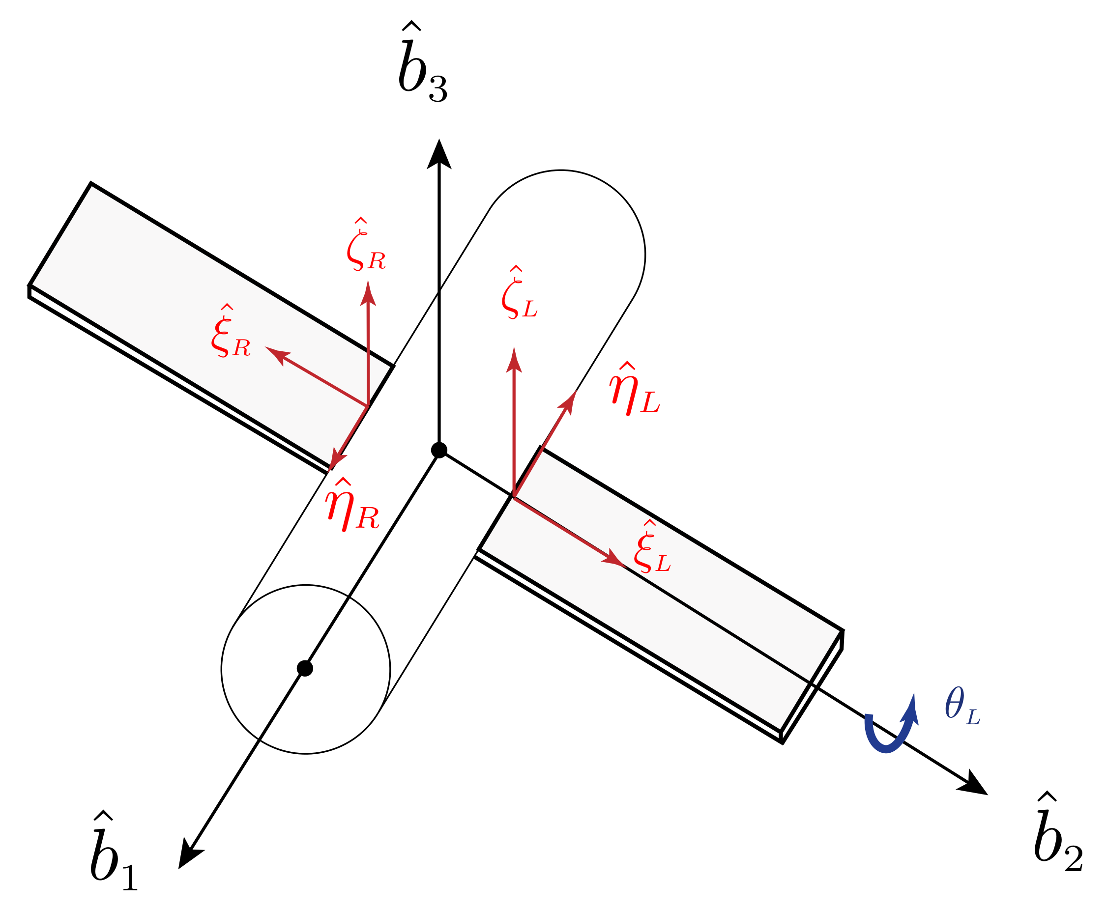
The spacecraft to control is composed of three main bodies (the central bus and two solar panels) which are connected to each other through revolute joints. The bus is modeled as a three-axial rigid body. The solar panels are able to rotate about their axes and they can be oriented properly toward the Sun during the maneuver. In Figure 1, the scheme of the satellite with the relevant reference frames is reported.
In the absence of elastic displacements and rotation of the solar panels, the inertia matrix of the entire spacecraft, resolved in the body-fixed reference frame, with respect to its center of mass, is taken from [19] and is
The inertial and geometric characteristics of the solar panels are reported in Table 1, where m is the mass, L the length, h the width, and the inertia cross section of the solar panel. Note that, due to the large aspect ratio of the panels defined as , their dynamic behavior is very similar to that of beam-like structures, where the first modal shapes are pure bending modes. In this study, a carbon Fiber Reinforced Polymer (CFRP) is considered, to represent the structure of the panels with an equivalent Young’s modulus = 72 GPa. Table 2 reports the first three natural frequencies (in rad/sec).
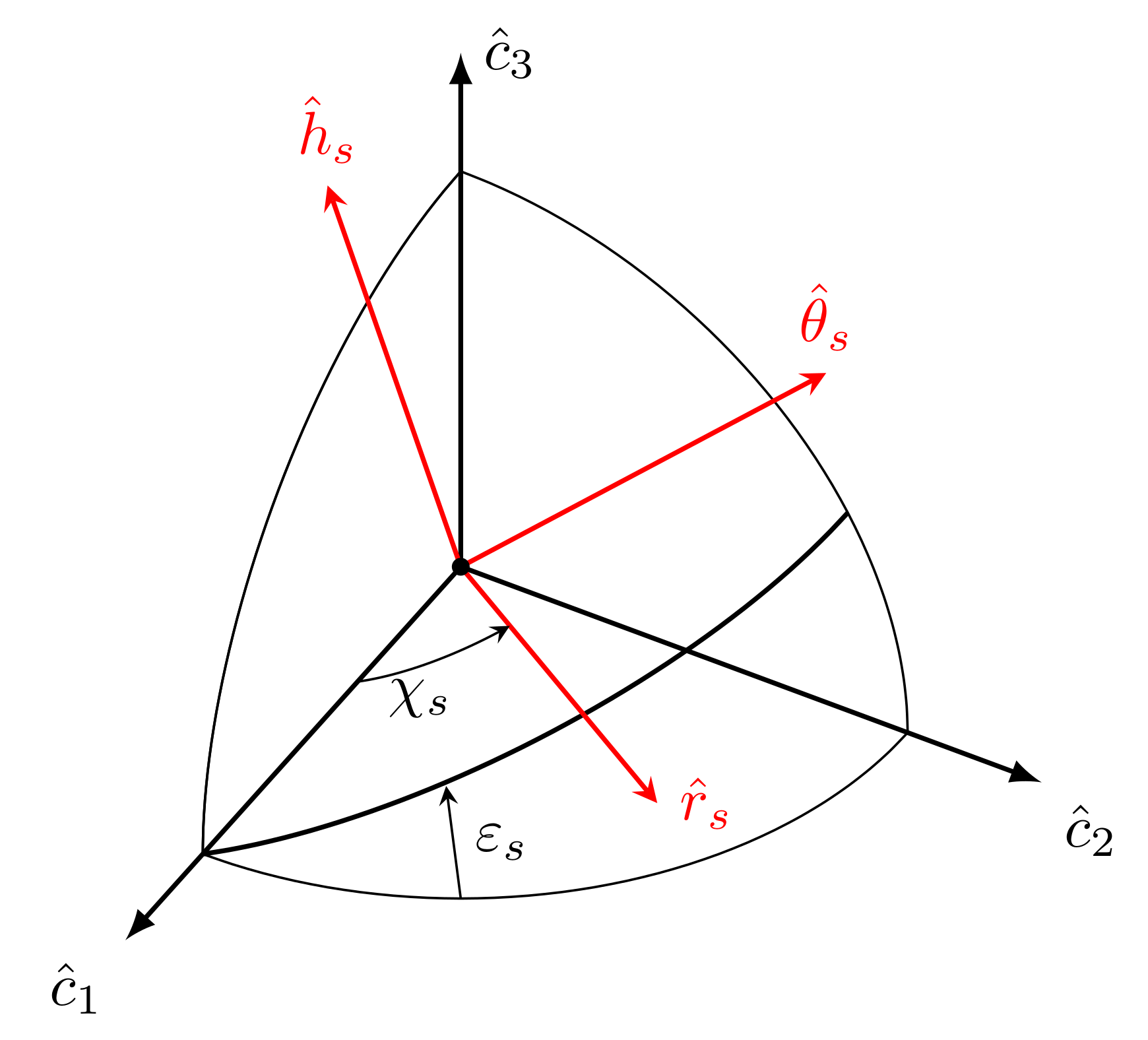
As previously mentioned, the solar panels are able to rotate with respect to the central bus. Hence, different reference frames and rotation matrices must be introduced to define the spacecraft attitude and the rotation of the solar panels. The first reference system is the Earth Centered Inertial (ECI) frame and the second system is the body-fixed frame, which is attached to the spacecraft and centered at its center of mass. These frames are associated with vectrices and , respectively. The last two reference frames, associated with and , are introduced in order to describe the rotation of the solar panels with respect to the bus of the satellite. They correspond to the two solar panels and are centered at the revolute joints. Figure 1 depicts the schematic of the satellite and the relevant reference frames. The bus is assumed to be a cylinder with a diameter m. The vectrices, associated with the reference frames, are
The relations between the reference frames are written in terms of elementary rotations,
where denotes a generic counterclockwise rotation about axis i by angle , whereas and are the two angles of the revolute joints associated with the left and the right solar panel, respectively.
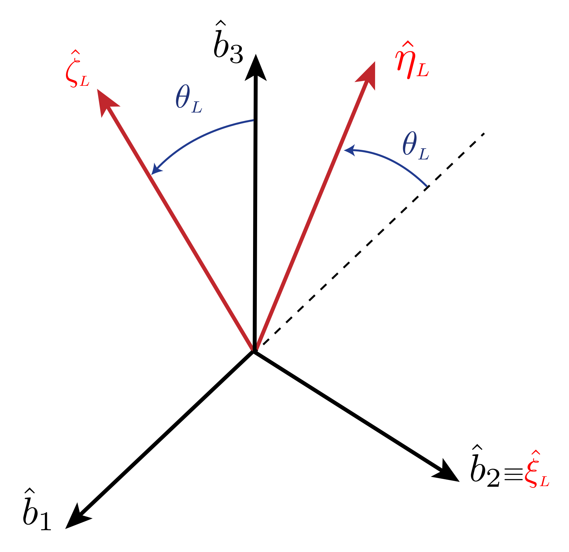
In order to clarify the kinematics of the system, Figure 2 illustrates the rotation about the axis of the left solar panel. The rotation of the right solar panel is symmetrical and described by angle about axis .
2.1. Flexible Appendages
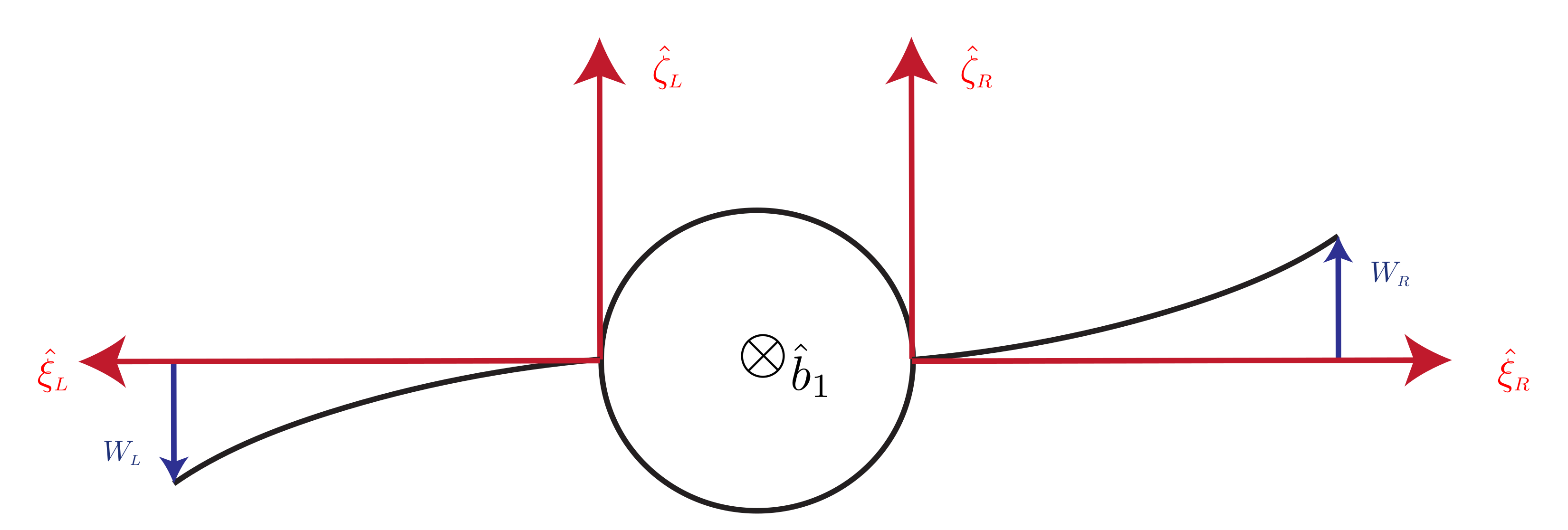
For elastic bodies, the “structure” must be introduced through a linear operator [w], which transforms the small structural displacement w, referred to the body reference frame, to structural forces acting on the generic point of the body [17]. In the present work, the dynamics of the solar arrays are described using beam-like models. This hypothesis can be considered valid since the ratio between the length of the solar panel and its width is >10 so the elastic displacements behave like the ones of a clamped-free flexural beam. The assumption of a “small” displacement leads to the possibility to express the elastic displacements w as a combination of the eigenmodes of vibration,
where is the coordinate of a generic point of the undeformed body, referred to the body axes of the solar panel, () are the eigenmodes of vibration, and the coefficient (t) must be determined. In order to clarify the elastic behavior of the system, Figure 3 portrays a sketch of the deformation of the solar panels.
2.2. Actuators
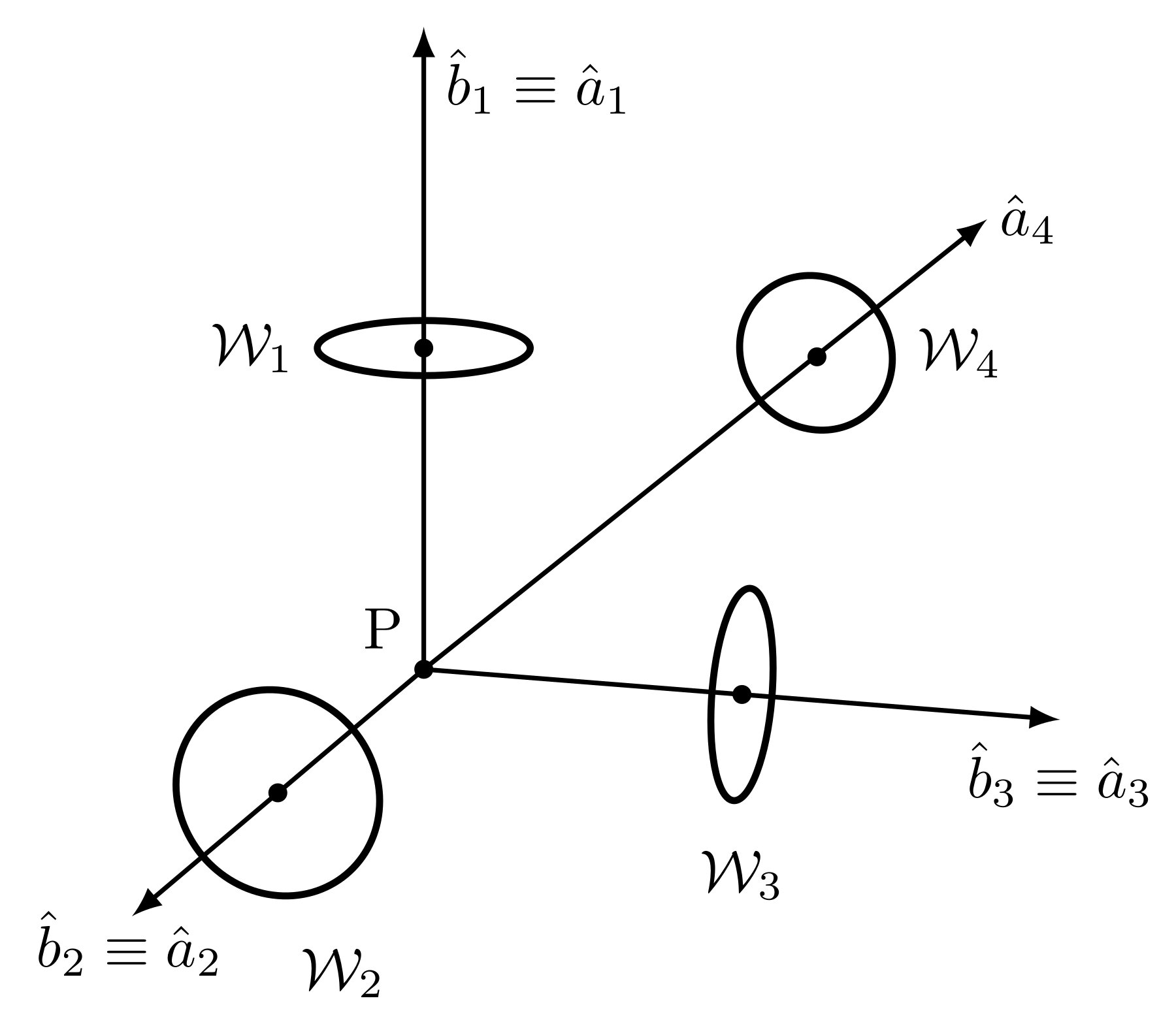
The attitude control action is actuated by means of four reaction wheels, arranged in an ortho-skew configuration (cf. Figure 4). Three devices have axes aligned with the principal inertia axes of the vehicle, whereas the fourth wheel has a skewed orientation, to partially compensate possible failures of the other devices.
Using the standard methodology of Eulerian attitude dynamics [20,21],the actual torque due to the array of reaction wheels and transferred to the vehicle is
where represents a -vector that collects the torque components along the body axes, is the skew-symmetric matrix associated with the components (along the body axes) of the angular velocity of the spacecraft, whereas
In Equations (10)–(12), is the axial angular velocity of wheel i relative to the spacecraft, is the related time derivative, and is the axial inertia moment of wheel i. Finally, if denotes the unit vector aligned with the axis of wheel i, then includes its components along the principal inertia axes of the vehicle. The actual torque must be as close as possible to the commanded torque , which is yielded by the attitude control algorithm (cf. Section 4). This task is demanded to the steering law. In order to obtain a convenient, closed-form steering law, Equation (9) is simplified by assuming that the angular velocity of the spacecraft is sufficiently small, i.e.,
As a result, the torque provided by the array of reaction wheels, simplifies to , and must equal the commanded torque ,
Starting from a given commanded torque , the objective is in finding such that . The problem involves three equations and four unknowns, and can be solved with the use of the Moore–Penrose pseudoinverse,
The preceding steering law minimizes the magnitude of the vector , while enforcing the contraint . The steering law (15) works only if matrix is nonsingular. This condition is satisfied if at least three columns of A are linearly independent, and this is the case with the ortho-skew arrangement. However, the real actuator dynamics corresponds to the actual torque reported in Equation (9), which differs from the commanded one by the term . To get more realistic results, the actual torque given by Equation (9) is included in the numerical simulations, while obtaining the required time derivatives from the steering law (15).
3. Spacecraft Attitude Dynamics with Flexibility
The spacecraft, initially modeled as a rigid body, has an instantaneous orientation associated with the body reference frame . In this study, the instantaneous attitude is referred to and is described through the direction cosine matrix. The attitude of the spacecraft is identified by , which is a rotation matrix such that . The kinematics equation for R is
Under the (approximating) assumption that the center of mass C does not move during the maneuver, the attitude dynamics equations are decoupled from the trajectory equations, and are given by
In Equation (17), is the vector that contains the sum of all external torques referred to the center of mass of the entire spacecraft, vector is the actual torque, and is the inertia matrix with respect to C. All these vectors are resolved in .
When the solar panels are modeled as flexible bodies, flexural degrees of freedom must be introduced, together with the related dynamics equations. By using the multibody formulation and after considerable algebra, not reported for the sake of brevity, the fully nonlinear governing equations for the spacecraft dynamics is obtained in matrix form,
Vectors and have dimensions appropriate to the context, i.e., ; their first three components coincide with those of and . Vector contains nonlinear (gyroscopic, centrifugal and reactions) terms, derived by the multbody formulation. Finally, is the second derivative of the state vector defined as
In Equation (19), () represents the angular acceleration around the j-th spacecraft body axis and () are the second derivatives of the amplitudes of the modal shapes of the right and left solar panels, respectively, whereas n is the number of modes assumed as representative for the purpose of describing the elastic displacements. Finally, M, K, and C are respectively the generalized mass, stiffness and damping matrices of the assembled spacecraft. It is worth noting that the matrix M is time-varying. In fact, due to the presence of the coupling terms between the rotational motion and the flexible dynamics, M depends on the amplitude of the modal shape and on the time-varying orientation of the solar panels with respect to the rigid central bus [23]. The expressions of M, K, and C are
where is the inertia matrix with respect to the center of mass, which is time-varying because it includes the modal shapes [24] and the rotation of the solar panels (cf. Section 5). S is the matrix of the rotation modal participation factors (coupled with rigid motion), is the identity matrix, is a diagonal matrix containing the squared angular frequencies of the solar panels as cantilivered to the satellite, and is the diagonal matrix of the k-th damping factor of the corresponding elastic mode.
4. Inertia-Free Nonlinear Attitude Control
In this research, the commanded torque is identified by using the algorithm presented in [4,25], which does not require a perfect knowledge of the inertia matrix. This approach is based on the Lyapunov method and employs the rotation matrix as the attitude representation.
The desired (commanded) attitude is associated with vectrix . The attitude control algorithm aims at determining the control torque such that the actual attitude of the spacecraft, associated with , pursues the commanded orientation, identified by the rotation matrix . In this study, a pointing maneuver is considered, and the commanded frame is chosen as coincident with the inertial reference frame . As a result, . The commanded torque is obtained by using the algorithm presented in [4,25], rewritten in simplified form for the case of a pointing maneuver,
Equation (21) represents a feedback control law, which supplies the commanded torque in terms of the variables R and . In Equation (21), is a constant, positive quantity and is a constant, diagonal, positive-definite matrix, whereas is the estimate of . The proof of stability of the preceding feedback law is reported in [4,25] and is omitted in this work. The inertia-estimator is governed by
In Equation (22), Q is a diagonal positive definite matrix while is a -vector that collects the six independent entries of the estimated inertia matrix. L is an operator which takes a -vector as the input and returns a -matrix as the output, i.e.,
The symbols () denote the diagonal terms of , which is an arbitrary, positive definite matrix, whereas vector is related to the displacement of the actual attitude matrix R from ,
The symbol represents the i-th column vector of the canonical basis.
Gain selection takes advantage of the following formulas, [4,25]:
where , , and are the three instantaneous angular velocity components. The two constant parameters and are written in terms of a positive quantity () and maximum torque magnitude [25],
The parameter plays an important role in the algorithm. In fact, it affects the transient behavior of the dynamical system at hand, and is related to the relative weight of the proportional and the derivative terms in the feedback control law.
5. Optimal Solar Panel Rotation
Matrix M and vector in Equation (18) depend explicitly on the joint variables , , , , , . During the attitude maneuver, the solar panels are rotated to minimize the angle between the normal to the solar panels and the direction of the Sun. To do this, the direction of the Sun, resolved in the ECI-frame , must be defined. Let and denote respectively the angle between the equatorial plane and the ecliptic plane (ecliptic obliquity) and the solar ecliptic longitude (i.e., the angle between the vernal axis and the Earth–Sun line). Let be the geocentric ecliptic reference frame. The relation between and , shown in Figure 5, is
The rotation matrix is given by two consecutive rotations: a counterclockwise rotation about axis 1 by angle , followed by a counterclockwise rotation about axis 3 by angle ,
It is worth noting that the angle varies very slowly in time and obeys
The term is assumed constant and denotes the angular velocity of the Sun in its motion relative to the Earth; represents one sidereal year.
The unit vector that identifies the direction of the Sun in the inertial reference frame is
The time derivative of is given by
This unit vector can be resolved in the body-fixed reference frame ,
where vector contains the components of in ,
Using Equation (33) and the kinematics equation of direction cosines, one can evaluate the time derivative of ,
Let represent the rotation matrix that relates the body frame and the left solar panel,
The normal to the left solar panel corresponds to the third row of the rotation matrix , i.e.,
To evaluate the angle between the normal to the left solar panel and the Sun direction, unit vector , reported in Equation (38), is projected into the inertial frame,
The symbol denotes the scalar product between the two unit vectors,
Since the solar panel must be oriented as much as possible toward the Sun, the maximum value of is sought,
leading to
Once is known its time derivative is computed, while is assumed to be zero, since varies very slowly,
Of course, the right panel must move in a similar way, i.e., its normal must remain parallel to the axis orthogonal to the left panel. Because axes and are aligned and with opposite directions, .
6. Numerical Simulations
This section includes the results of the numerical simulations for the large reorientation maneuver of interest. The final, desired attitude is related to the initial attitude by an eigenangle of 180 degrees. The final objective consists of reaching the desired attitude with zero angular velocity.
The initial conditions, in terms of rotation matrix and angular velocity of the spacecraft, are
6.1. Slewing Maneuver with Ideal Actuation
In this subsection, two different simulations are presented:
- slow slewing maneuver;
- fast slewing maneuver.
In these two preliminary simulations, the main goal is in verifying the structural behavior of the spacecraft when it is subject to different control torques. In both cases, the dynamics is simplified in the sense that the actuators are not modeled. This means that the actual torque, which affects the spacecraft dynamics, coincides with the commanded torque. In Section 6.2, the actuator modeling will be included in additional numerical simulations.
Figure 6, Figure 7, Figure 8 and Figure 9 illustrate the time evolution of the angular rate components, the eigenangle, and the torque components during the slow slewing maneuver, with fixed solar panels. From inspection of Figure 6, it is apparent that the angular velocity components never exceed 0.5 deg/sec and drop to zero after 4000 sec, which is the duration of the transient period. The eigenangle starts at 180 deg and decreases to 0 in about 4000 sec as well. This means that the entire reorientation maneuver takes about 4000 sec. The torque components have a magnitude not exceeding 1 Nm. Figure 9 portrays the time histories of the tip displacements of the solar panels. Their order of magnitude is modest, and therefore one can conclude that the solar panels are weakly excited during the slow reorientation maneuver. This circumstance is a consequence of the relatively small values of the applied torque.
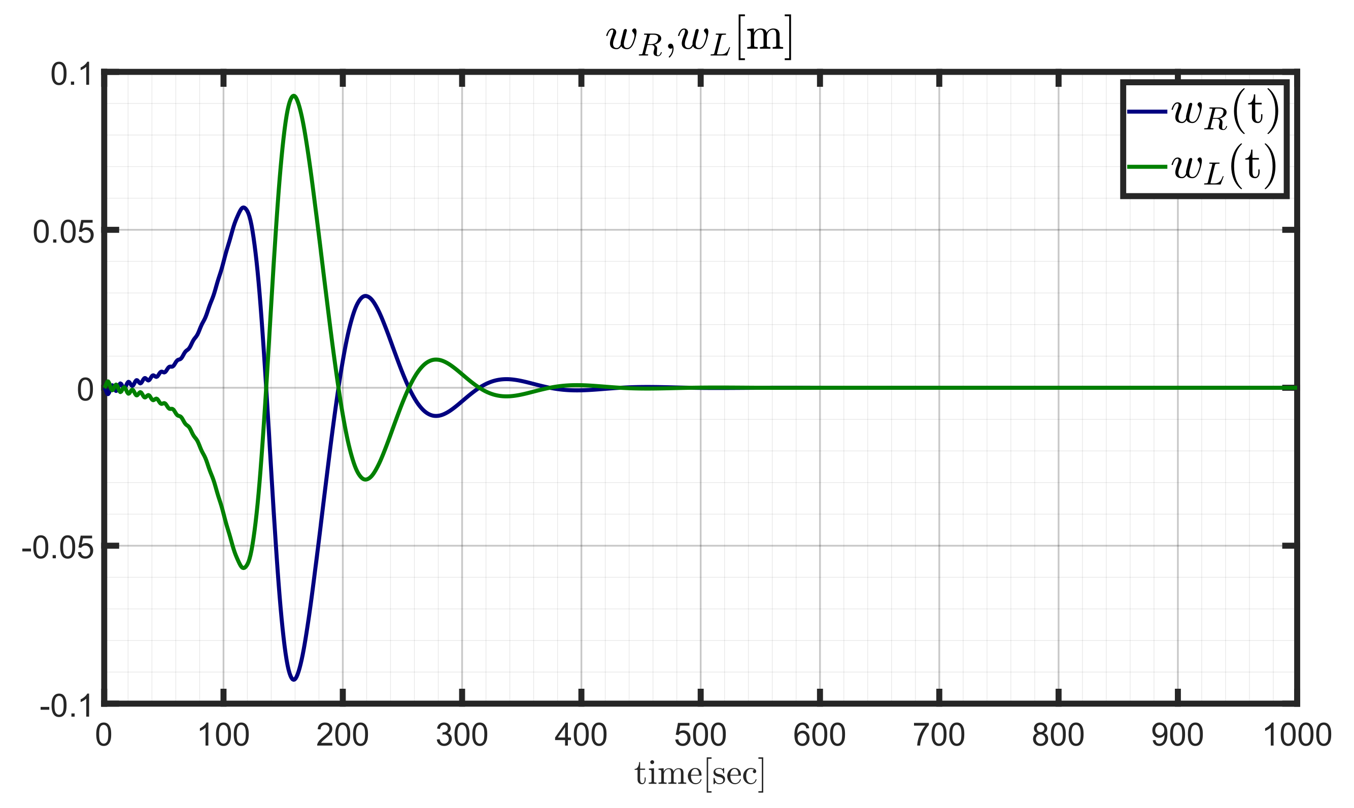
Figure 10, Figure 11, Figure 12 and Figure 13 illustrate the time evolution of the angular rate components, the eigenangle, and the torque components during the fast slewing maneuver, with fixed solar panels. From the inspection of Figure 10, it is apparent that the angular velocity component 1 undergoes much larger oscillations with respect to the remaining components, and approaches 4 deg/sec. All of them turn out to drop to 0 in about 400 sec. The eigenangle starts at 180 deg and decreases to 0 in about 400 sec as well. This means that the entire reorientation maneuver takes about 400 sec, which is a much shorter period compared to the slow slewing maneuver. The torque components, illustrated in Figure 12, reach much larger values with respect to the preceding case (tens of Nm), and this explains the reduction of the time needed to complete the reorientation maneuver. Unlike the previous case, the tip displacements reach values of a few centimeters. Though expected, this is a relevant result because it provides a quantitative estimation of the tip displacements due to flexibility, in terms of applied torque and duration of the slewing maneuver.
6.2. Slewing Maneuver with Actuation
In this subsection, the actuator dynamics is modeled, using the data reported in Table 3. Moreover, the solar panels are assumed to rotate, to get a proper orientation with respect to the Sun. The dynamical framework considered in this subsection presents further relevant complexities. First, the actuation devices have maximum values of and . Moreover, the actual torque differs from the commanded torque, and this must not compromise the achievement of the final, desired attitude, in a reasonable time. At the initial time, all the reaction wheels are at rest with respect to the spacecraft; therefore,
Matrix Q, which is related to the inertia estimator dynamics (22), includes large values if the knowledge of the mass distribution of the spacecraft is satisfactory. Conversely, small values imply poor knowledge of the spacecraft mass distribution. In this research, Q is set to
The gains, introduced in Section 4, are set to
The choice of is related to the transient duration and is the result of extensive numerical search, using the method described in [24].
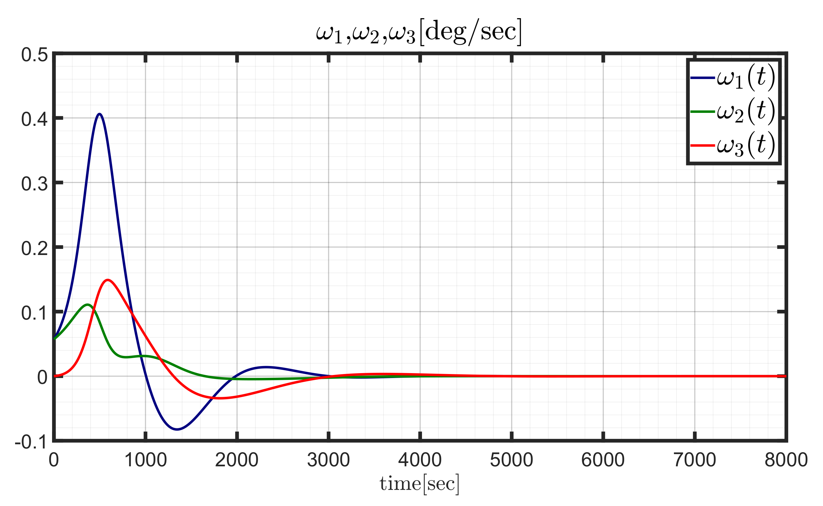
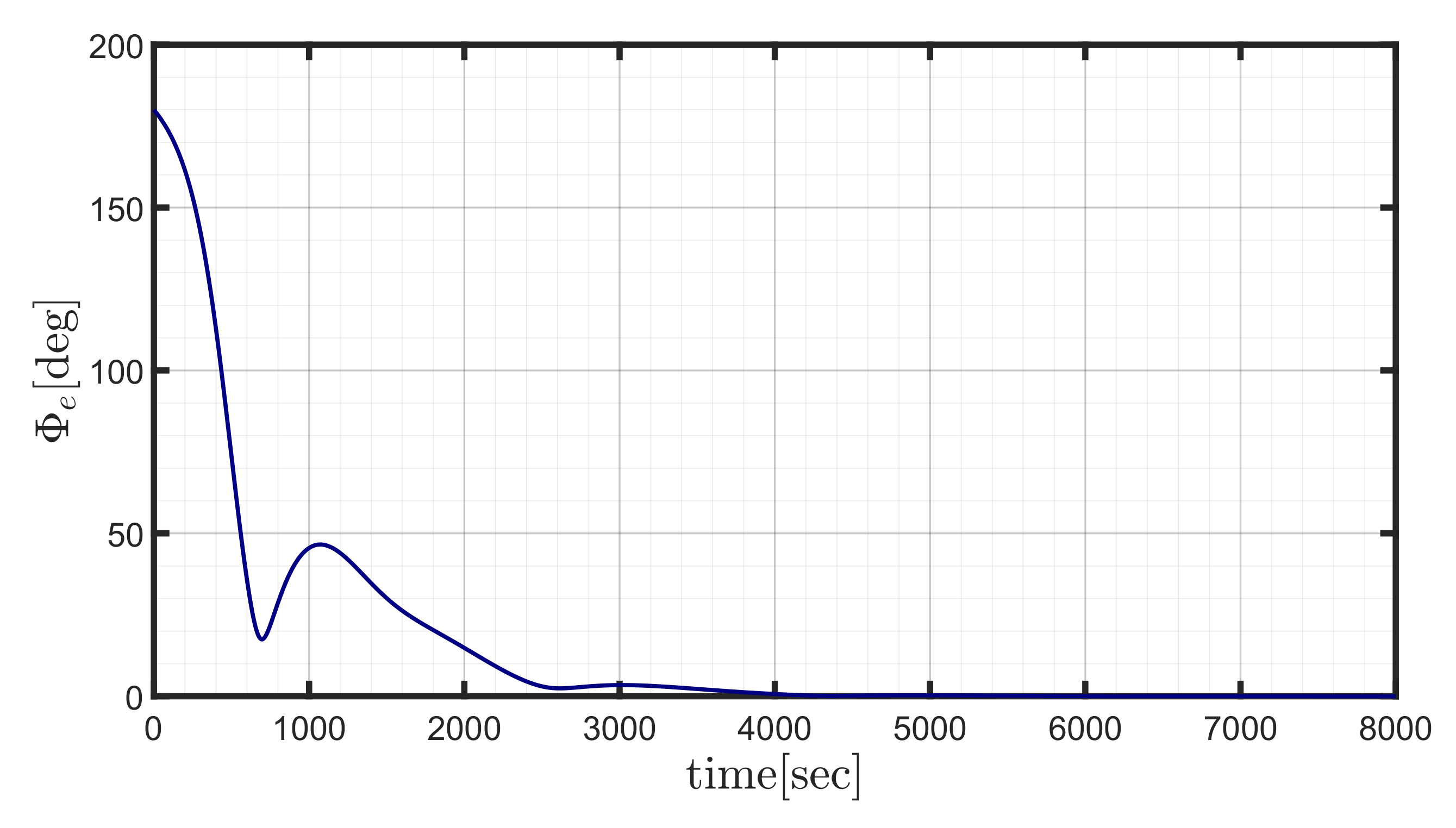
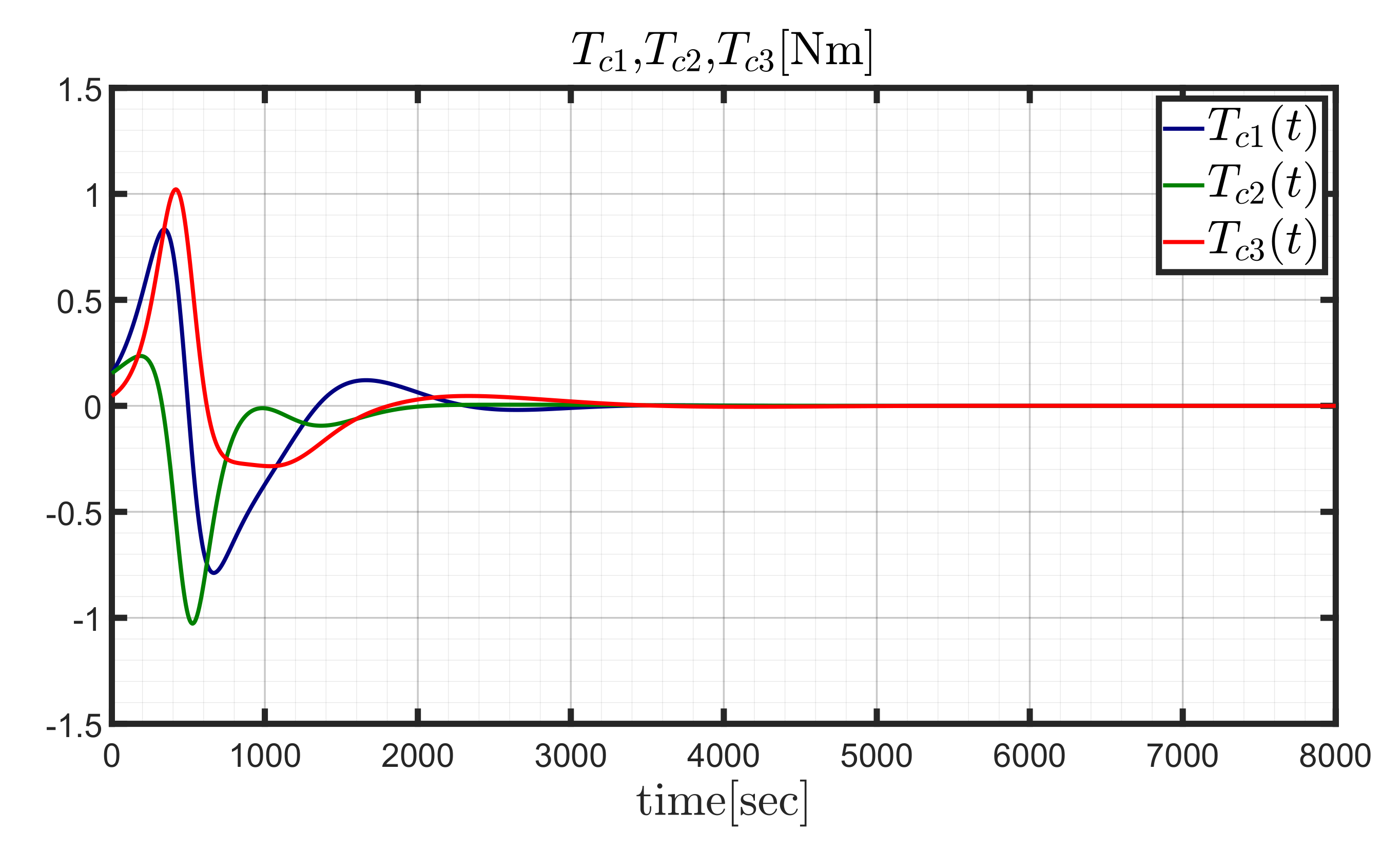
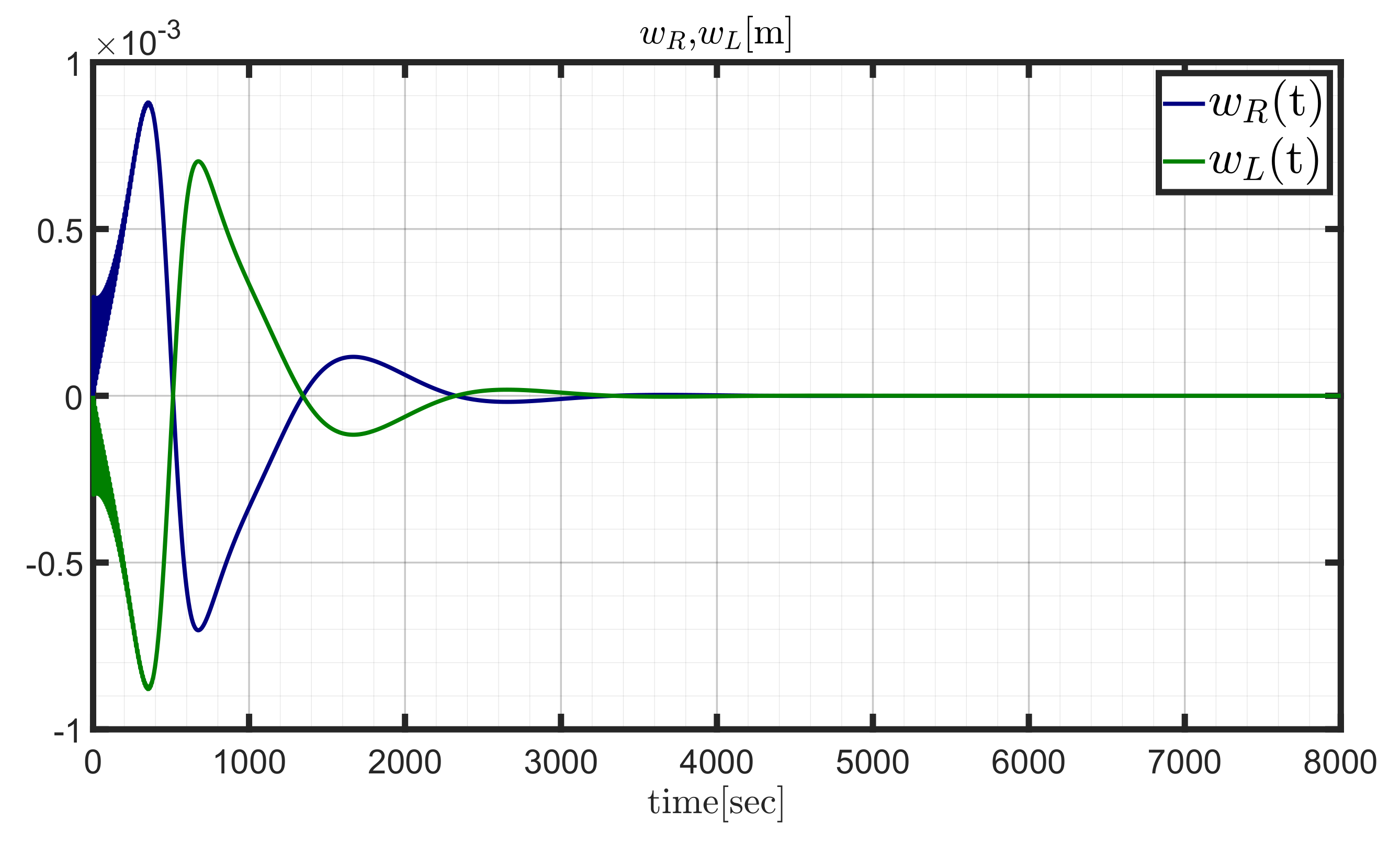
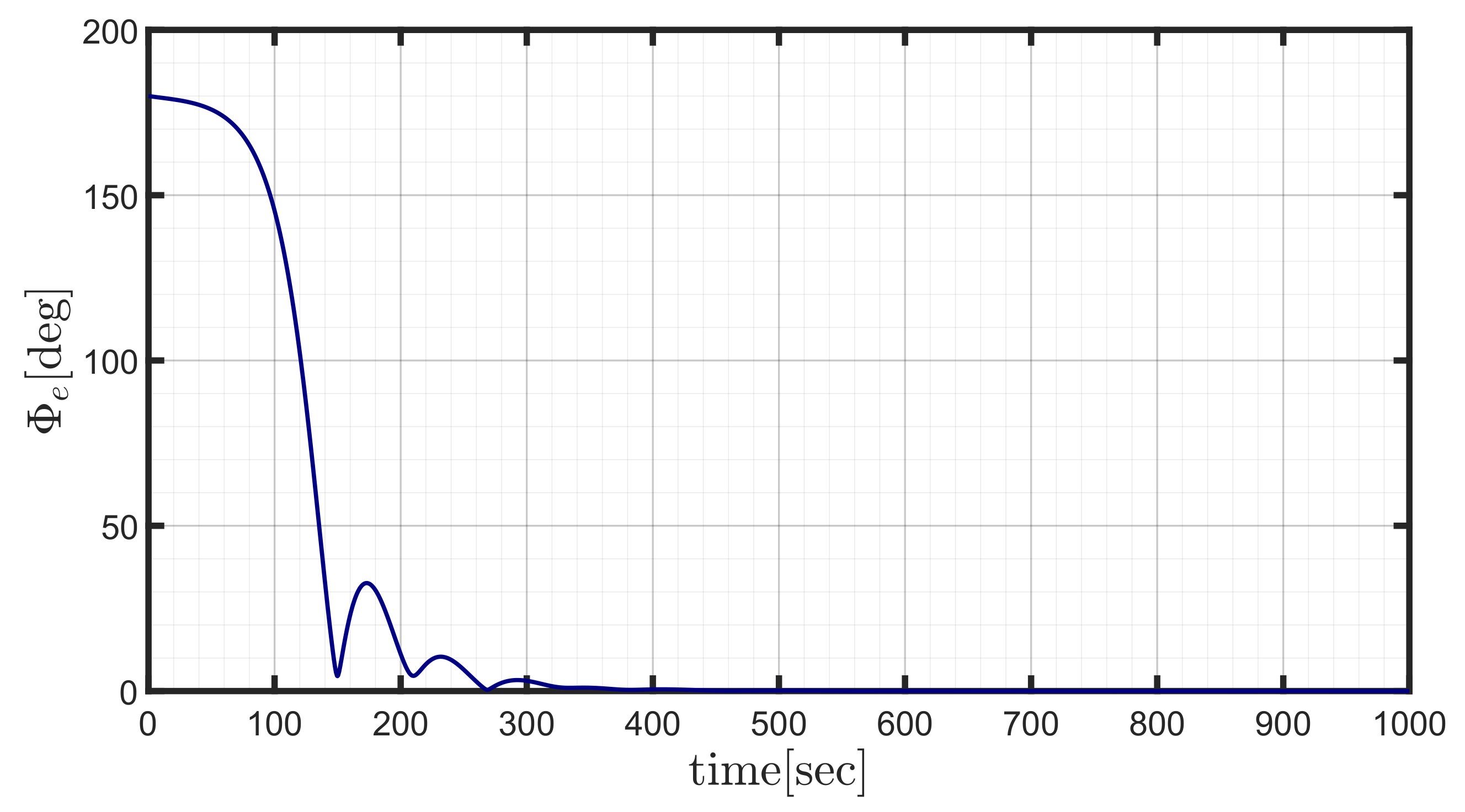
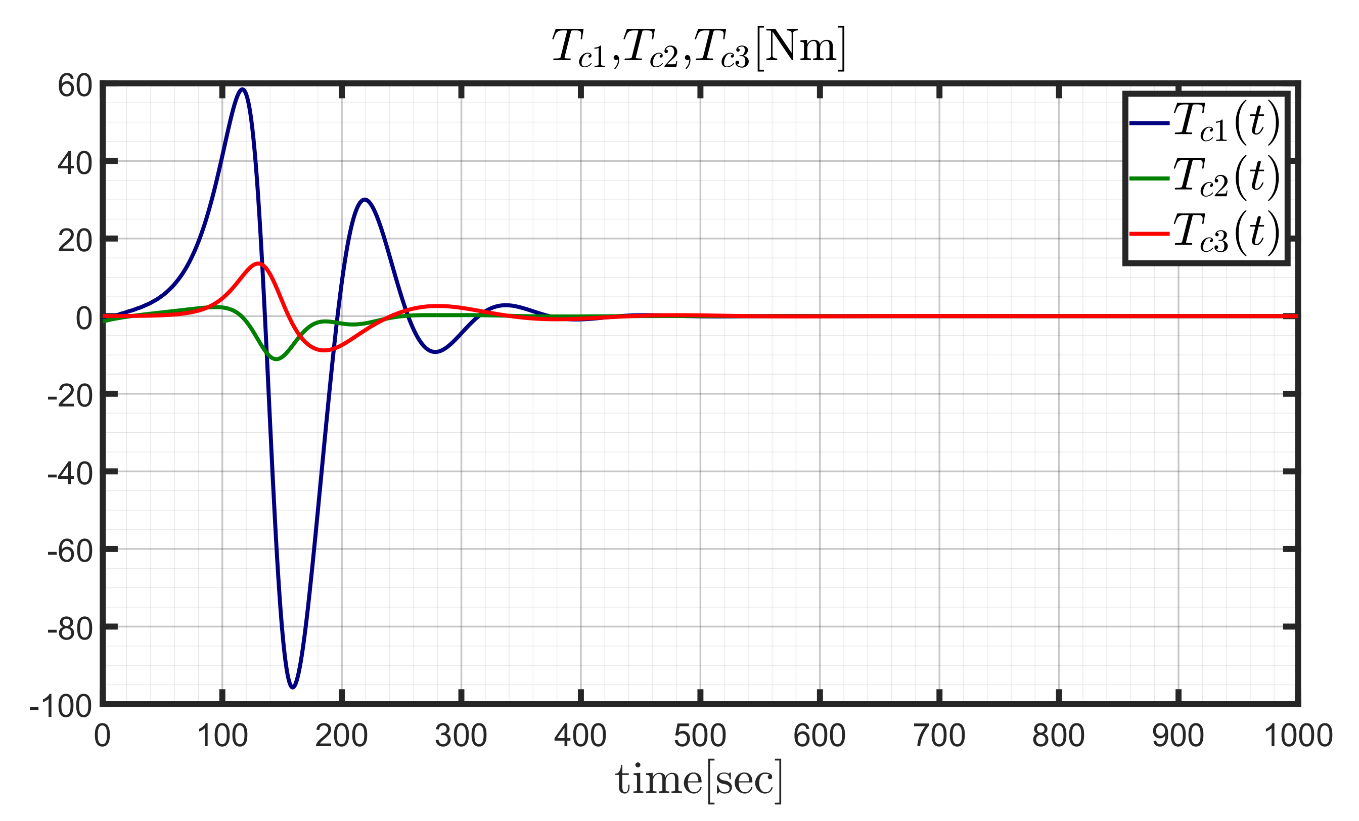
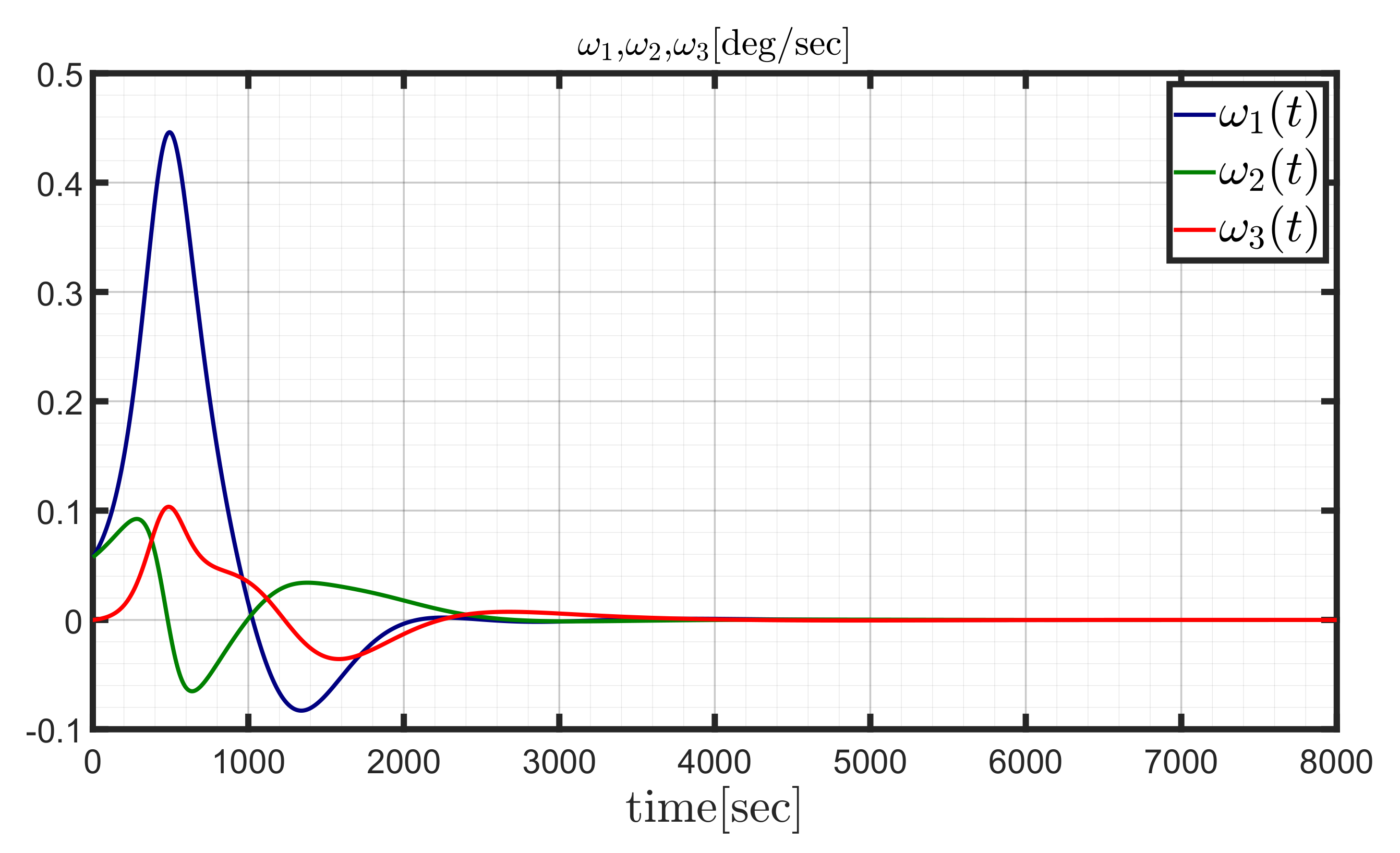
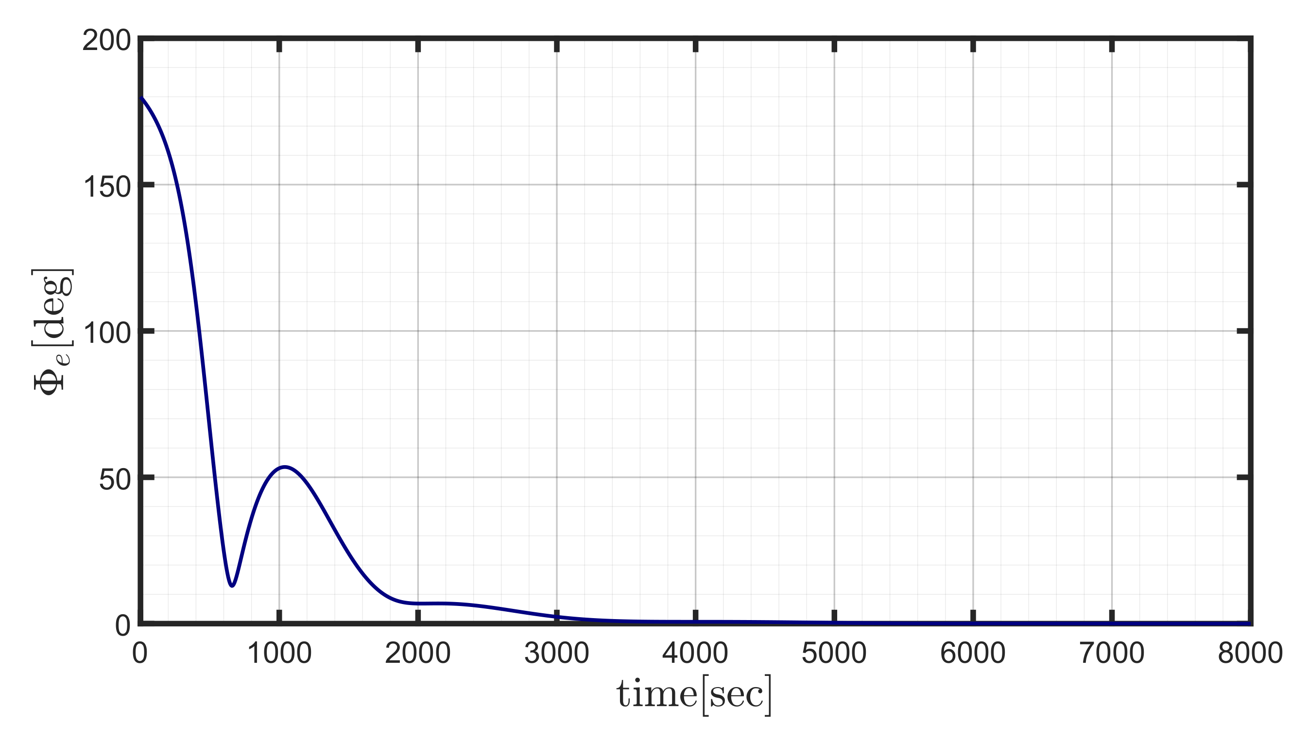
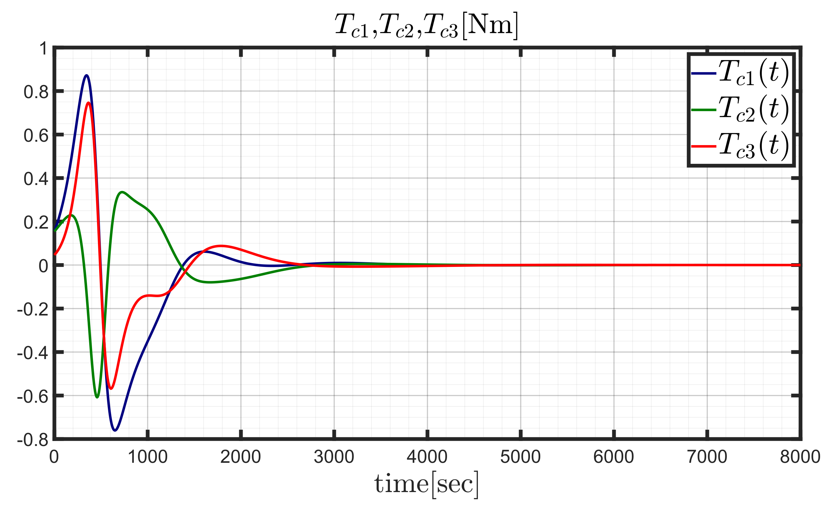
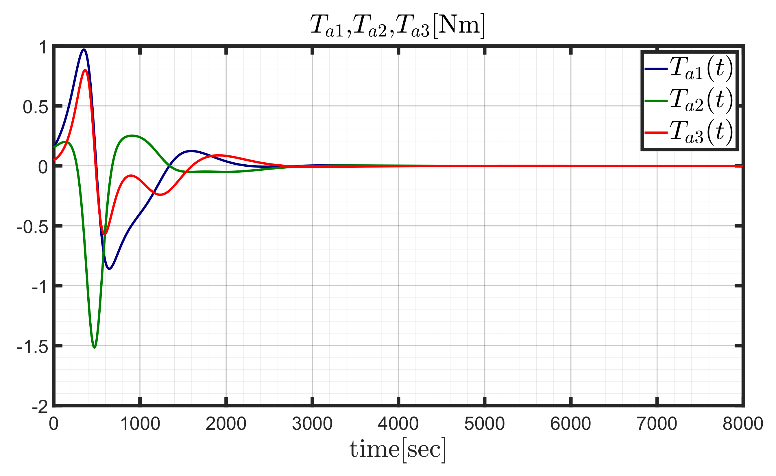
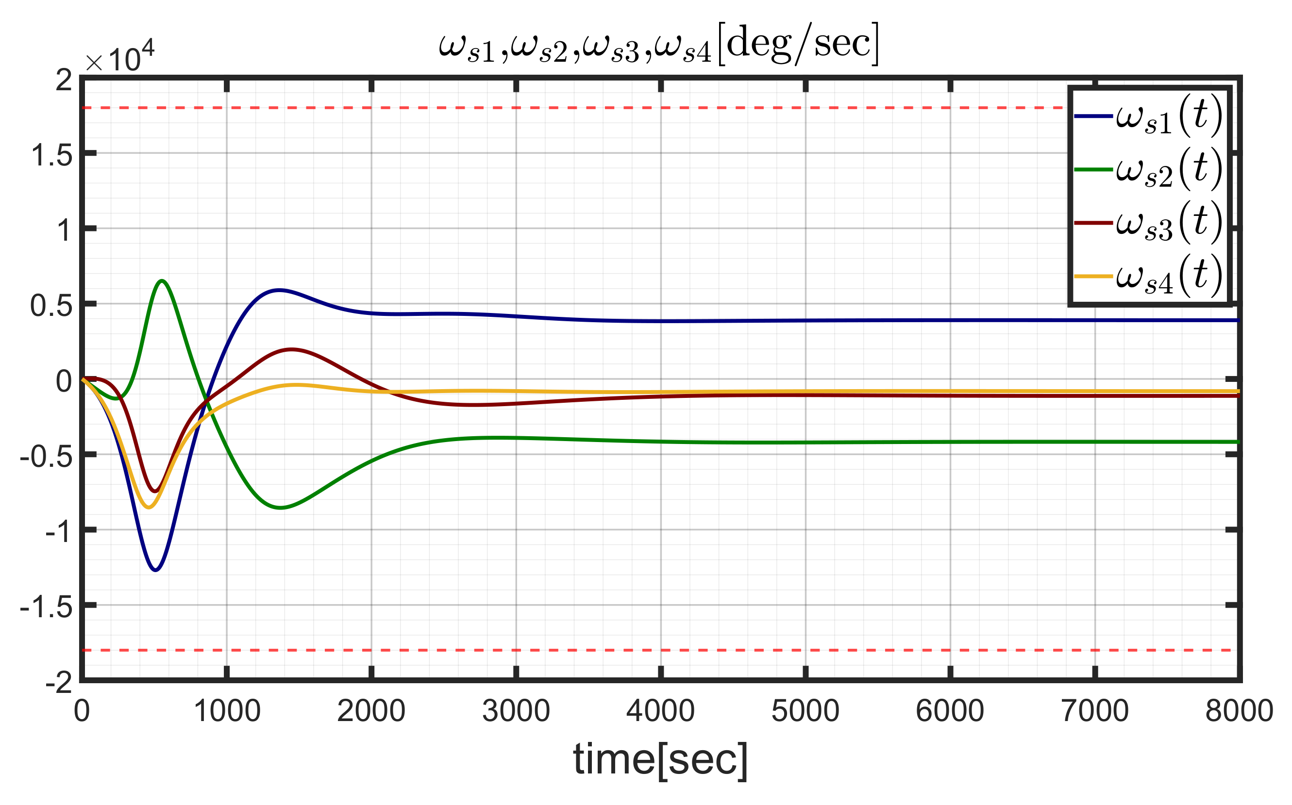
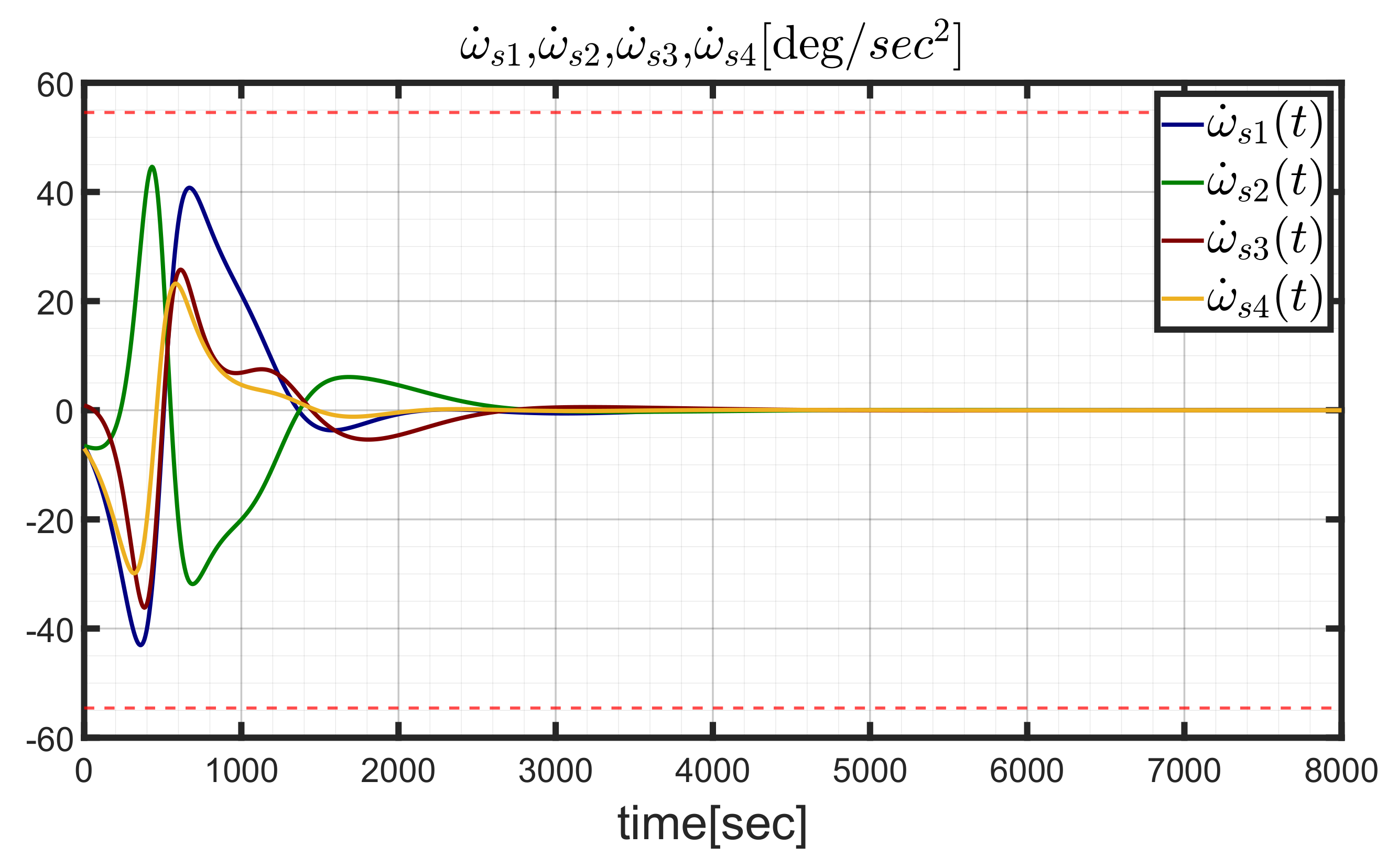
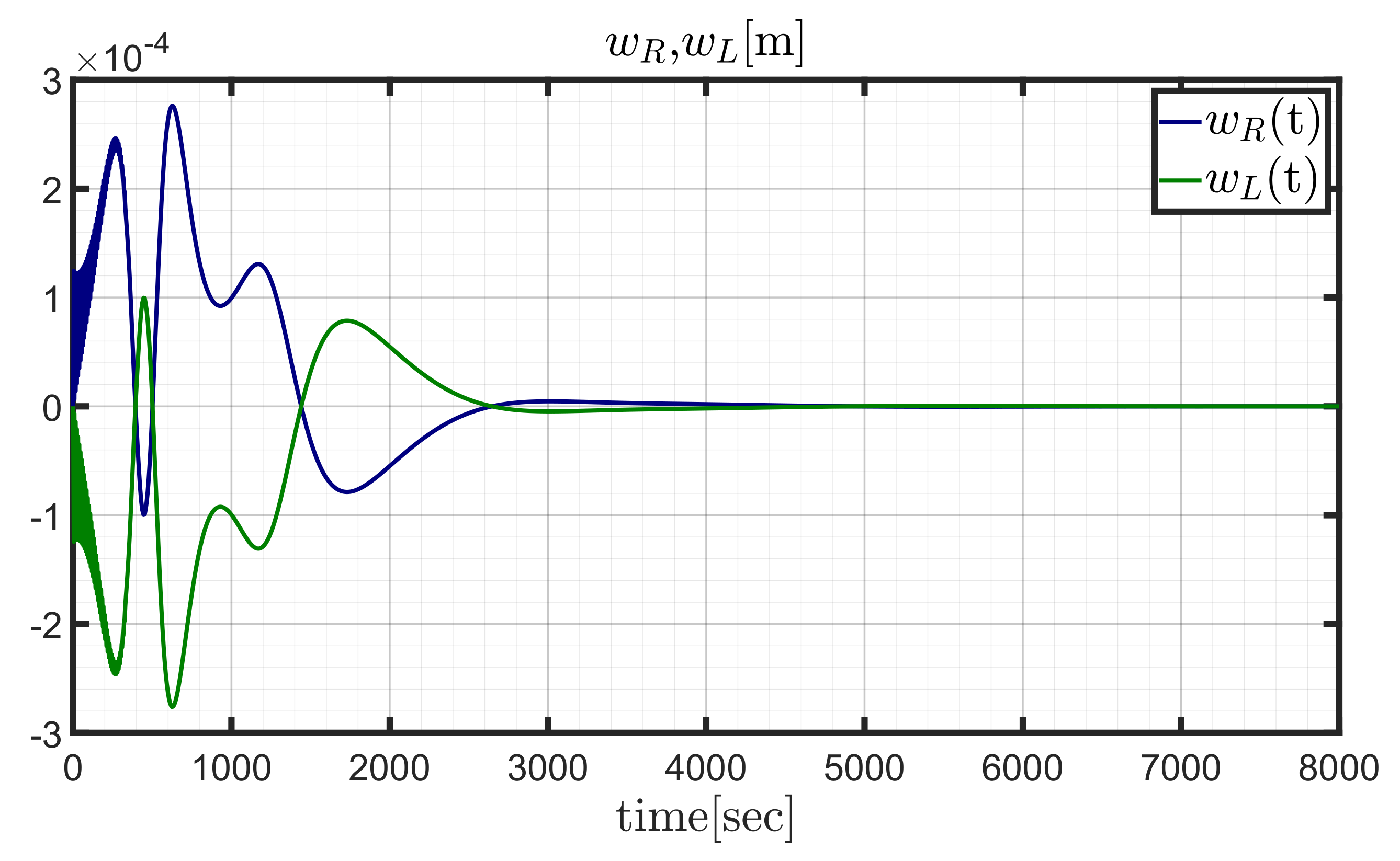
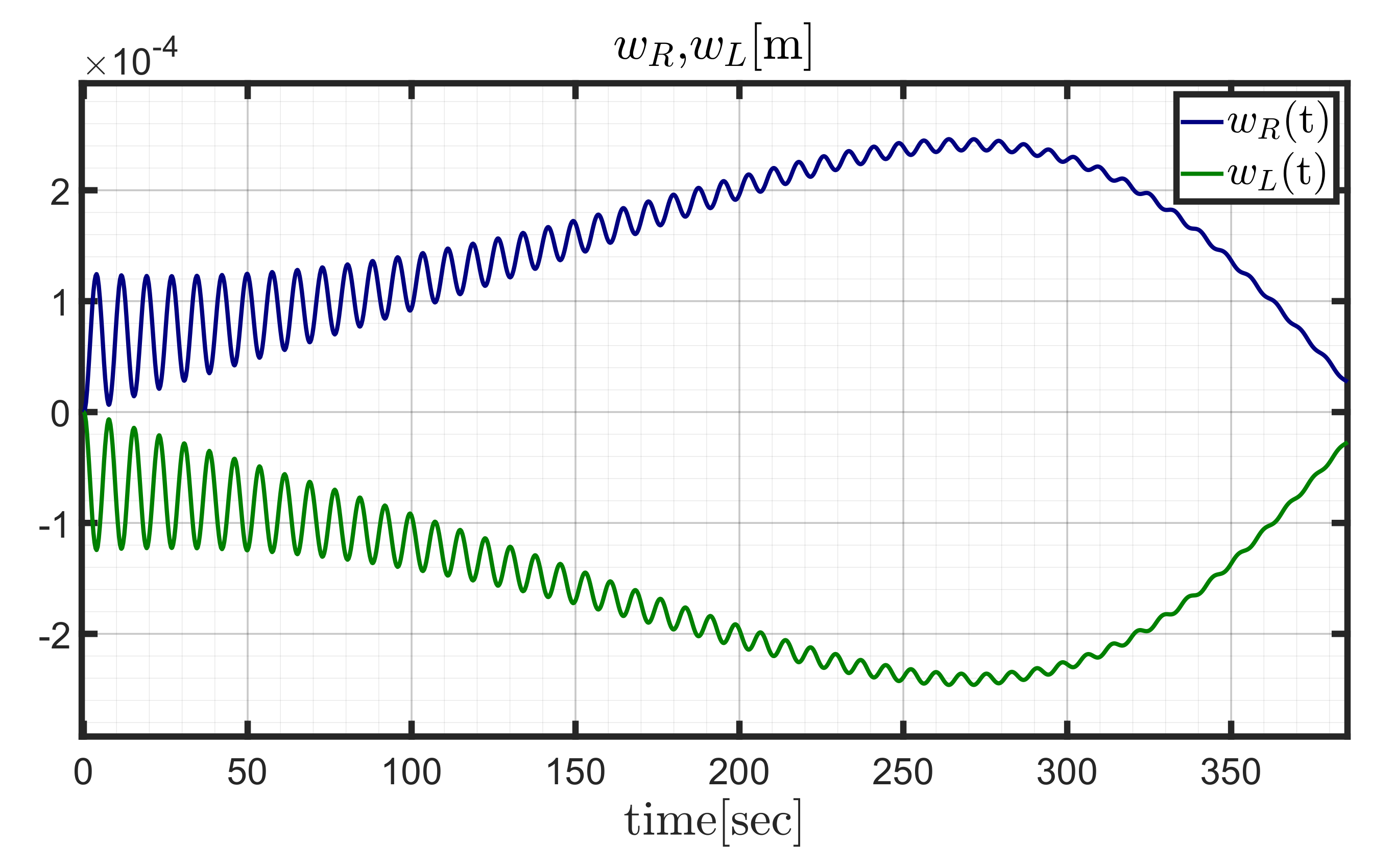
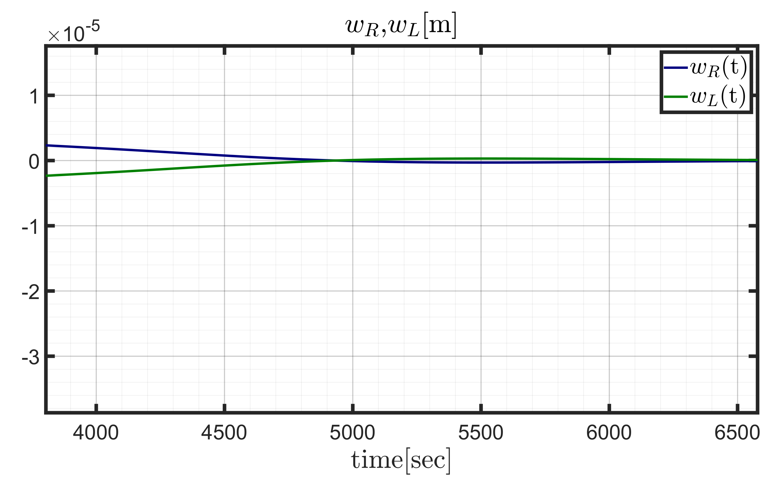
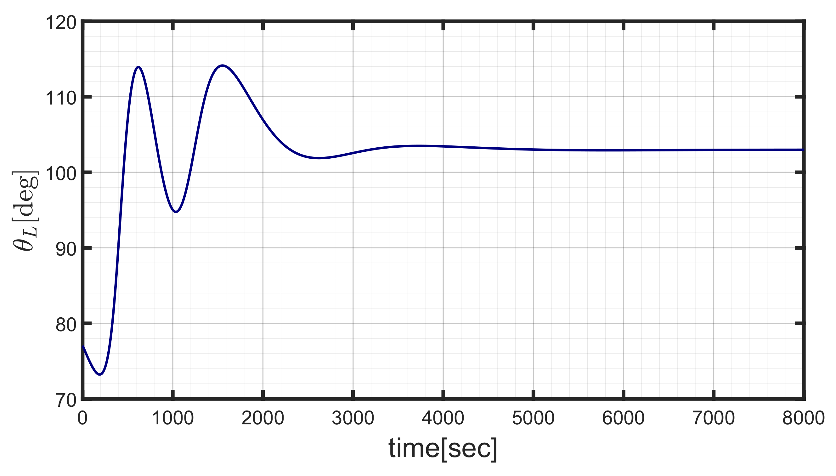
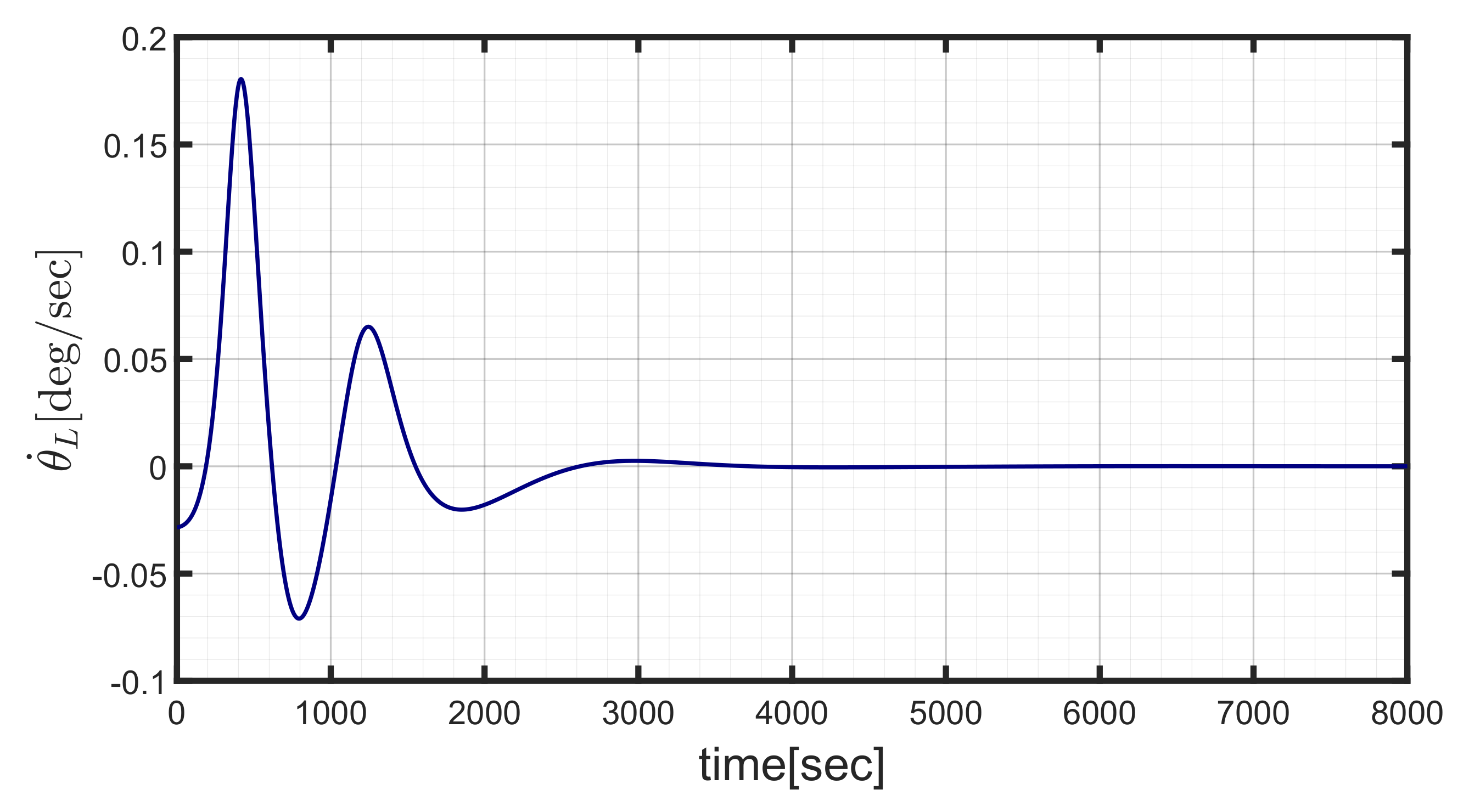
Figure 14 depicts the time histories of the angular rate components, never exceeding 0.5 deg/sec, pointing out the total duration of the maneuver, i.e., about 4000 sec. Figure 15 shows that the eigenangle starts at 180 deg and drops to 0 in about 4000 sec as well. Figure 16 and Figure 17 illustrate the the components of the commanded and actual torque, respectively. Although these torque components exceed 0.8 Nm, which is the maximum torque supplied by a single reaction wheel, the actual torque , which is the real torque generated and transferred to the vehicle by an array of reaction wheels, depends on additional terms other than (cf. Equation (9)). This explains the difference between the time histories portrayed in Figure 16 and Figure 17. Figure 18 and Figure 19 depict the time histories of the angular velocities and accelerations of the four devices. Inspection of these figures reveals that saturation, associated with the red dashed lines, never occurs. The elastic deformations are shown in Figure 20, which illustrates the tip displacements. These are obtained through a linear combination of the modal shapes, according to Equation (8), and reach modest values, less than 1 mm. Figure 21 and Figure 22 portray the zoom on the initial and final time histories of the tip displacements. The initial oscillations are related to the excitation of the modal shapes. Moreover, from inspection of Figure 22, it is apparent that the elastic displacement is not exactly zero, although the maneuver has finished. This is due to the fact that the attitude control algorithm is designed making reference to the rigid body dynamics and does not consider structural flexibility. In any case, the elastic deformations reach modest values (less than 1 mm) and play a marginal role in the reorientation maneuver, thanks to a suitable choice of the actuation devices and the related available control torque. Finally, Figure 23 and Figure 24 illustrate the time histories of (t) and (t). These variables, computed with the algorithm described in Section 5, are such that the angle between the Sun direction and the normal to the panel is minimized. Obviously, under the assumption of neglecting the very slow time variation of the Sun direction, the angle of the solar panel tends to a constant value once the maneuver has been completed.
In conclusion, the spacecraft proves to be able to perform the large reorientation maneuver of interest with modest tip displacements and in reasonable time, despite the low torque levels provided by the actuators. This proves that the feedback law (21), designed for rigid bodies with the assumption of ideal actuation, is effective in the control and actuation architecture described in this research, i.e., when flexible appendages and actuation dynamics are also included in the dynamical modeling of the spacecraft of interest.
7. Conclusions
This study considers slewing maneuvers of large satellites, equipped with flexible solar panels and reaction wheels as the actuation devices. As a first contribution, the Euler–Newton formulation is employed to construct a suitable model for the spacecraft of interest. The solar panels are modeled as flexural beams, using the modal decomposition technique, which represents a suitable approach that avoids finite-element analysis, provided that elastic displacements remain sufficiently limited. An inertia-free nonlinear attitude control algorithm, which employs rotation matrices and enjoys quasi-global stability properties without requiring any information on the spacecraft inertia matrix, is implemented and tested. Slow and fast slewing maneuvers are simulated. This leads to identifying the required torque components, whose values drive the choice of the actuation device. Moreover, this preliminary analysis points out that the elastic displacements remain modest, and therefore this research proves that internal structural damping is sufficient to get a sufficiently quick reduction of the oscillations’ amplitude. Then, the two panels are assumed to rotate. This study defines an optimal rotation strategy for the solar panels, capable of maximizing the power storage during the reorientation maneuver. As a further contribution, actuator dynamics are also included in the dynamical modeling, and the actual torque transferred to the vehicle no longer coincides with the commanded torque supplied by the nonlinear control algorithm. Nevertheless, this research demonstrates that the slewing maneuver can be successfully completed in reasonable time and without any saturation of the actuation devices, while the elastic displacements remain modest, in spite of the panel rotation aimed at pursuing the Sun direction. This result proves that slewing maneuvers can be effectively performed through the use of a feedback law designed for attitude control of rigid bodies and not requiring any information on the spacecraft mass distribution, even in the presence of rotating flexible solar panels. Future work can regard the extension of nonlinear attitude control based on rotation matrices to flexible space structures through feedback compensation of elastic displacements, for the purpose of performing fast, large reorientation maneuvers, e.g. with the use of control momentum gyroscopes.
Author Contributions
Conceptualization, M.P. (Massimo Posani), M.P. (Mauro Pontani) and P.G.; methodology, M.P. (Mauro Pontani) and P.G.; software, M.P. (Massimo Posani); validation, M.P. (Mauro Pontani) and P.G.; formal analysis, M.P. (Massimo Posani); investigation, M.P. (Massimo Posani); resources, M.P. (Massimo Posani), M.P. (Mauro Pontani) and P.G.; data curation, M.P. (Massimo Posani); writing—original draft preparation, M.P. (Massimo Posani); writing—review and editing, M.P. (Mauro Pontani) and P.G.; visualization, M.P. (Massimo Posani); supervision, M.P. (Mauro Pontani) and P.G.; project administration, M.P. (Massimo Posani), M.P. (Mauro Pontani) and P.G.; funding acquisition, M.P. (Mauro Pontani) and P.G. All authors have read and agreed to the published version of the manuscript.
Funding
This research was funded by Sapienza Università di Roma Grant No. RM11715C77620E5B (Progetti Ateneo Medi 2019). The APC was funded by Sapienza Università di Roma Grant No. RM11715C77620E5B (Progetti Ateneo Medi 2019).
Institutional Review Board Statement
Not applicable.
Informed Consent Statement
Not applicable.
Conflicts of Interest
The authors declare no conflict of interest.
Abbreviations
The following abbreviations are used in this manuscript:
| ECI | Earth Centered Inertial |
| RWs | Reaction Wheels |
References
- Wie, B.; Barba, P.M. Quaternion feedback for spacecraft large angle maneuvers. AIAA J. Guid. Control Dyn. 1985, 8, 360–365. [Google Scholar] [CrossRef]
- Weiss, H. Quaternion-based rate/attitude tracking system with application to gimbal attitude control. J. Guid. Control Dyn. 1993, 16, 609–616. [Google Scholar] [CrossRef]
- Napoli, I.; Pontani, M. A new guidance and control architecture for orbit docking using feedback linearization. In Proceedings of the 72nd International Astronautical Congress, Dubai, United Arab Emirates, 25–29 October 2021. [Google Scholar]
- Sanyal, A.; Fosbury, A.; Chaturvedi, N.; Bernstein, D.S. Inertia-free spacecraft attitude tracking with disturbance rejection and almost global stabilization. Aiaa J. Guid. Control Dyn. 2009, 32, 1167–1178. [Google Scholar] [CrossRef] [Green Version]
- Weiss, A.; Yang, X.; Kolmanovsky, I.; Bernstein, D.S. Inertia-free spacecraft attitude control with reaction-wheel actuation. In Proceedings of the AIAA Guidance, Navigation, and Control Conference, Toronto, ON, Canada, 2–5 August 2010. [Google Scholar]
- Leve, F.A.; Hamilton, B.J.; Peck, M.A. Spacecraft Momentum Control Systems; Springer: Berlin/Heidelberg, Germany, 2015. [Google Scholar]
- Liu, F.; Jin, D. A high-efficient finite difference method for flexible manipulator with boundary feedback control. Space Sci. Technol. 2021, 2021, 9874563. [Google Scholar] [CrossRef]
- Tahmasebi, M.; Esmailzadeh, S.M. Modeling and co-simulating of a large flexible satellites with three reaction wheels in ADAMS and MATLAB. Int. J. Dyn. Control 2018, 6, 79–88. [Google Scholar] [CrossRef]
- Cao, L.; Xiao, B.; Golestani, M. Robust fixed-time attitude stabilization control of flexible spacecraft with actuator uncertainty. Nonlinear Dyn. 2020, 100, 2505–2519. [Google Scholar] [CrossRef]
- Ford, K.A.; Hall, C.D. Flexible spacecraft reorientations using gimbaled momentum wheels. Adv. Astronaut. Sci. 1998, 97, 1895–1914. [Google Scholar] [CrossRef]
- Ford, K.A. Reorientations of Flexible Spacecraft Using Momentum Exchange Devices. Ph.D. Thesis, Department of Aeronautics and Astronautics, Air Force Institute of Technology, Wright-Patterson Air Force Base (WPAFB), Dayton, OH, USA, 1997. [Google Scholar]
- Nudehi, S.S.; Farooq, U.; Alasty, A.; Issa, J. Satellite attitude control using three reaction wheels. In Proceedings of the American Control Conference, Westin, Seattle Hotel, Seattle, WA, USA, 11–13 June 2008. [Google Scholar]
- Gasbarri, P.; Monti, R.; Sabatini, M. Very large space structures: Nonlinear control and robustness to structural uncertainties. Acta Astronaut. 2014, 93, 252–265. [Google Scholar] [CrossRef]
- Gasbarri, P.; Monti, R.; De Angelis, C.; Sabatini, M. Effects of uncertainties and flexible dynamic contributions on the control of a spacecraft full-coupled model. Acta Astronaut. 2014, 94, 515–526. [Google Scholar] [CrossRef]
- Angeletti, F.; Iannelli, P.; Gasbarri, P.; Sabatini, M. End-to-end design of a robust attitude control and vibration suppression system for large space smart structures. Acta Astronaut. 2021, 187, 416–428. [Google Scholar] [CrossRef]
- Gasbarri, P. A two-dimensional approach to multibody free dynamics in space environment. Acta Astronaut. 2002, 51, 831–842. [Google Scholar] [CrossRef]
- Santini, P.; Gasbarri, P. General background and approach to multibody dynamics for space applications. Acta Astronaut. 2009, 64, 1224–1251. [Google Scholar] [CrossRef]
- Gasbarri, P.; Sabatini, M.; Pisculli, A. Dynamic modeling and stability parametric analysis of a flexible spacecraft with fuel slosh. Acta Astronaut. 2016, 127, 141–159. [Google Scholar] [CrossRef]
- Nurre, G.S.; Sharkey, J.P.; Nelson, J.D.; Bradley, A.J. Preservicing mission, on-orbit modifications to Hubble Space Telescope pointing control system. AIAA J. Guid. Control Dyn. 1995, 18, 222–229. [Google Scholar] [CrossRef]
- Pontani, M. Lecture Notes of the Course “Advanced Spacecraft Dynamics”; Sapienza Università di Roma: Rome, Italy, 2021. [Google Scholar]
- Hughes, P.C. Spacecraft Attitude Dynamics; Wiley: New York, NY, USA, 1986; Reprint Dover: New York, NY, USA, 2008. [Google Scholar]
- Beals, G.A.; Crum, R.C.; Dougherty, H.J.; Hegel, D.K.; Kelley, J.L.; Rodden, J.J. Hubble Space Telescope precision pointing control system. AIAA J. Guid. Control Dyn. 1988, 11, 119–123. [Google Scholar] [CrossRef]
- Pisculli, A.; Gasbarri, P. A minimum state multibody/FEM approach for modeling flexible orbiting space systems. Acta Astronaut. 2015, 110, 324–340. [Google Scholar] [CrossRef]
- Posani, M. Nonlinear Attitude Control of Complex Space Systems. Master’s Thesis, Sapienza Università di Roma, Rome, Italy, 2021. [Google Scholar]
- Cruz, G.; Yang, X.; Weiss, A.; Kolmanovsky, I.; Bernstein, D.S. Torque-saturated, inertia-free spacecraft attitude control. In Proceedings of the AIAA Guidance, Navigation, and Control Conference, Portland, OR, USA, 8–11 August 2011. [Google Scholar]
Figure 1.
Schematic of the satellite and reference frames for = = 0.

Figure 2.
rotation of the left solar panel.

Figure 3.
Sketch of the solar panels deformation.

Figure 4.
Ortho-skew arrangement of the four reaction wheels.

Figure 5.
Sun direction in the ECI-frame.

Figure 6.
(t),(t),(t)[deg/sec] during the slow slewing maneuver.

Figure 7.
(t)[deg] during the slow slewing maneuver.

Figure 8.
(t),(t),(t)[Nm] during the slow slewing maneuver.

Figure 9.
Tip displacements (t),(t)[m] during the slow slewing maneuver.

Figure 10.
(t),(t),(t)[deg/sec] during the fast slewing maneuver.

Figure 11.
(t)[deg] during the fast slewing maneuver.

Figure 12.
(t),(t),(t)[Nm] during the fast slewing maneuver.

Figure 13.
Tip displacements (t),(t)[m] during the fast slewing maneuver.

Figure 14.
(t),(t),(t)[deg/sec] during the slewing maneuver with actuation.

Figure 15.
(t)[deg] during the slewing maneuver with actuation.

Figure 16.
(t),(t),(t)[Nm] during the slewing maneuver with actuation.

Figure 17.
(t),(t),(t)[Nm] during the slewing maneuver with actuation.

Figure 18.
(t),(t),(t),(t)[deg/sec] during the slewing maneuver.

Figure 19.
(t),(t),(t),(t)[deg/sec] during the slewing maneuver.

Figure 20.
Tip displacements (t),(t)[m] during the slewing maneuver.

Figure 21.
Zoom on the tip displacements (t),(t)[m] at the beginning of the maneuver.

Figure 22.
Zoom on the tip displacements (t),(t)[m] at the end of the maneuver.

Figure 23.
(t)[deg] during the slewing maneuver.

Figure 24.
(t)[deg/sec] during the slewing maneuver.


Table 1.
Panels data.
| m [kg] | L [m] | h[m] | [m] |
|---|---|---|---|
| 81 | 15 | 1.0 | 2.5 × |
Table 2.
First three natural frequencies of the beam-like solar panels.
| [rad/sec] | [rad/sec] | [rad/sec] |
|---|---|---|
| 0.7138 | 4.4711 | 12.5192 |
Table 3.
Characteristic parameters of each actuation device.
| [rpm] | [kg m] | [Nm] |
|---|---|---|
| 3000 | 0.84 | 0.8 |
Publisher’s Note: MDPI stays neutral with regard to jurisdictional claims in published maps and institutional affiliations. |
© 2022 by the authors. Licensee MDPI, Basel, Switzerland. This article is an open access article distributed under the terms and conditions of the Creative Commons Attribution (CC BY) license (https://creativecommons.org/licenses/by/4.0/).
Share and Cite
MDPI and ACS Style
Posani, M.; Pontani, M.; Gasbarri, P. Nonlinear Slewing Control of a Large Flexible Spacecraft Using Reaction Wheels. Aerospace 2022, 9, 244. https://0-doi-org.brum.beds.ac.uk/10.3390/aerospace9050244
AMA Style
Posani M, Pontani M, Gasbarri P. Nonlinear Slewing Control of a Large Flexible Spacecraft Using Reaction Wheels. Aerospace. 2022; 9(5):244. https://0-doi-org.brum.beds.ac.uk/10.3390/aerospace9050244
Chicago/Turabian StylePosani, Massimo, Mauro Pontani, and Paolo Gasbarri. 2022. "Nonlinear Slewing Control of a Large Flexible Spacecraft Using Reaction Wheels" Aerospace 9, no. 5: 244. https://0-doi-org.brum.beds.ac.uk/10.3390/aerospace9050244
Note that from the first issue of 2016, this journal uses article numbers instead of page numbers. See further details here.