
Real-Time Fuel Optimization and Guidance for Spacecraft Rendezvous and Docking

1
Aerospace System Engineering, University of Science and Technology, Daejeon 34113, Korea
2
Korea Aerospace Research Institute (KARI), Daejeon 34133, Korea
*
Author to whom correspondence should be addressed.
Aerospace 2022, 9(5), 276; https://0-doi-org.brum.beds.ac.uk/10.3390/aerospace9050276
Submission received: 20 April 2022
/
Revised: 17 May 2022
/
Accepted: 18 May 2022
/
Published: 20 May 2022
(This article belongs to the Topic Micro/Nano Satellite Technology, Systems and Components)
Abstract
:Autonomous rendezvous and docking (RVD) fuel optimization with field-of-view and obstacle avoidance constraints is a nonlinear and nonconvex optimization problem, making it computationally intensive for onboard computation on CubeSats. This paper proposes an RVD fuel optimization and guidance technique suitable for onboard computation on CubeSats, considering the shape, size and computational limitations of CubeSats. The computation time is reduced by dividing the guidance problem into separate orbit and attitude guidance problems, formulating the orbit guidance problem as a convex optimization problem by considering the CubeSat shape, and then solving the orbit guidance problem with a convex optimization solver and the attitude guidance problem analytically by exploiting the attitude geometry. The performance of the proposed guidance method is demonstrated through simulations, and the results are compared with those of conventional methods that perform orbit guidance optimization with attitude quaternion feedback control. The proposed method shows better performance, in terms of fuel efficiency, than conventional methods.
1. Introduction
Rendezvous and docking (RVD) is an important maneuver for space operations performed to accomplish tasks such as space rescue, on-orbit servicing, supply and assembly missions. Spacecraft RVD has long been a focus in the aerospace industry. Fuel optimization [1,2,3,4], time minimization [1,5], safety [6,7,8] and real-time implementation [2,9] are among the most well-studied topics in the literature. Fuel optimization and real-time implementability are particularly important for CubeSats.
Several methods have been proposed in the literature to solve the fuel-optimized guidance problem for RVD. These methods can be divided into two groups based on the approaches that they use to handle dynamic models. The first and more commonly used approach involves solving the orbit and attitude guidance problems for the coupled dynamic model as a single fuel optimization problem, while the other approach is to first optimize the orbit guidance and then apply attitude control subsequently.
For the coupled dynamic model approach, [1] used the direct collocation method to solve the minimum-energy and minimum-time rendezvous problem. In [3], a direct transcription method was used to obtain a tractable static program for the coupled translational and angular dynamics, and then a model predictive controller (MPC) was used to handle disturbances. Because of the large number of parameters, the coupled dynamic model approach is computationally intensive and hence less suited for onboard real-time implementation on a resource-constrained CubeSat computer.
The decoupled dynamic model approach has also been taken by some authors [10,11,12,13,14]; ref. [10] used linear quadratic control (LQC) for orbit trajectory optimization and a quaternion-based attitude controller for attitude maneuvering, while in [11], a single-thruster suboptimal trajectory was employed for the orbit trajectory, while geometric and nonlinear programming methods were used for attitude control. Although the decoupled dynamic model approach is computationally less intensive than the coupled dynamic model approach, for a multi-thruster configuration, depending on the attitude, the fuel expenditure can be higher in practice than what is calculated during trajectory optimization as a result of using more than one thruster. The articles that consider the decoupled dynamic model approach either optimize fuel based on the orbit trajectory without considering the attitude guidance at all [12], or they do not take into consideration the field of view and other constraints for the attitude [10,13,14]. In the latter case, during attitude maneuver, the spacecraft is aligned in such a manner that a single thruster is used to apply the required delta-v, which is the applied impulse per unit of the spacecraft mass [10].
In this research, a fast and fuel-efficient orbit and attitude guidance method is proposed for CubeSats with six thrusters. The proposed method decouples the guidance problem into an orbit energy optimization subproblem and an attitude fuel optimization subproblem. The CubeSat shape is used to formulate the collision avoidance constraints for the orbit optimization subproblem. A novel geometric approach is introduced to minimize the fuel loss in practice when multiple thrusters are applied. The geometry of the attitude vectors in space is used to analytically find the optimal attitude for reducing the computation time, which is hence best suited for real-time implementation. The performance of the proposed method is analyzed and demonstrated through simulations. Although the proposed guidance method is designed for CubeSats, it can be applied to other satellites by adapting the collision avoidance criterion to fit the relevant geometry.
The main contributions of this research are:
- Formulation of an orbit optimization problem that considers the shape of CubeSats;
- Analytical solution of the attitude guidance optimization problem;
- Collision avoidance method based on geometry of CubeSats.
This paper is organized as follows. Section 2 describes the coordinate frames of the RVD system and the chaser and target equations of motion. In Section 3, a continuous-time coupled orbit and attitude fuel optimization problem is formulated, and its discrete equivalent is found. Then, the proposed decoupled optimization problem is presented in Section 4. In Section 5, simulation case studies are presented, and the results are discussed. Finally, conclusions are presented in Section 6.
2. RVD Model
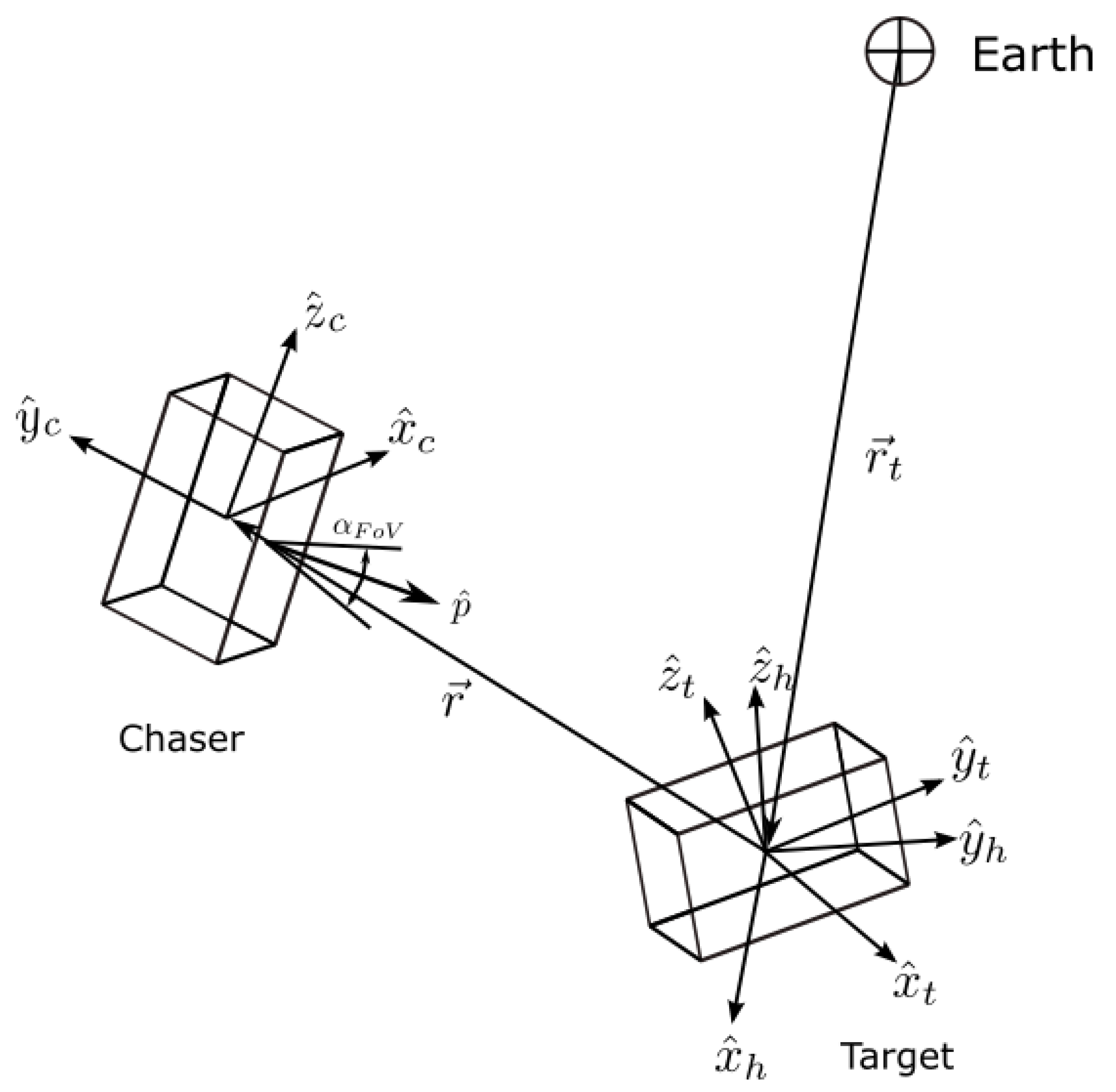
In this research, a chaser spacecraft equipped with three pairs of pulsed thrusters each aligned along the positive and negative directions of the principal axes of the spacecraft and three reaction wheels placed orthogonally is considered. It is assumed that the chaser flies on a near-circular low Earth orbit (LEO) and is to be docked to a target spacecraft with a known docking port position and attitude tumbling freely. A guidance profile for the chaser is to be generated in a Hill’s frame that is located at the center of the target, as shown in Figure 1.
Throughout this article, an overbar will be used to indicate a vector with more than three components, a vector sign will indicate a three-component vector, a hat will indicate a unit vector, and a bold symbol will indicate a matrix.
The Hill’s frame shown in Figure 1 has its component along the position vector of the target, lies along the orbit normal vector, and follows the right-hand rule.
2.1. Orbital Equations of Motion
The linear translation equations of motion of the chaser spacecraft have been given by [15], as shown in Equation (1), which is relative to the target spacecraft in a circular orbit described in the Hill’s frame.
where x, y and z are the position coordinates of the chaser relative to the target in the Hill’s frame. , and are the thrust forces of the chaser in the Hill’s frame. m is the mass of the chaser, , is the standard gravitational constant, and is the distance of the target from the center of the Earth in its circular orbit.
The continuous-time solution of Equation (2) is
where is the state transition matrix (STM) given by [16], as shown in Equation (4).
In Equation (2), the control input is continuous. Since the thrusters are pulsed, the integral term can be reduced to a summation term as follows:
In the above equation, N is the number of thruster burns, and is the delta-v required in Hill’s frame at the time of the k-th thruster burn. The delta-v is the amount of impluse per unit mass of the spacecraft.
Applying thruster burns at equal time intervals will cause to be equal for all intervals; then, Equation (3) becomes
Using Equation (6) for a single interval, the relation between any state and the previous state is found to be
where is the time interval between thruster burns.
2.2. Attitude Equations of Motion
The attitude kinematic equations of the chaser and target in the Hill’s frame are given by [17]
where is the quaternion vector in the Hill’s frame, and , and are the components of the angular velocities of the spacecraft relative to Hill’s frame in an inertial frame.
The attitude dynamics equations of the chaser spacecraft with reaction wheels are [15]
where is the chaser’s inertia matrix, is a vector of the reaction wheel angular momenta for the three wheels, is the angular velocity of he spacecraft in the inertial frame, and is the torque that the reaction wheels exert on the spacecraft body.
3. Fuel Optimization Problem
The fuel optimization problem considering the coupled orbit and attitude dynamics can be formulated as the minimization of the sum of all of the delta-v of each thruster subject to the orbital and attitude equations of motion, field-of-view constraints, safe distance constraints, bounds on the maximum delta-v and the initial and final states of the chaser.
3.1. Objective Function
The objective is to minimize the total delta-v required to perform the RVD motion. A minimum fuel cost function with the attitude quaternion and the states as the design variables is chosen:
where is the first norm and is the the delta-v required in the body frame.
3.2. Constraints
Equation (7) is an orbit constraint, and Equations (8) and (9) are the attitude kinematic and dynamic constraints, respectively.
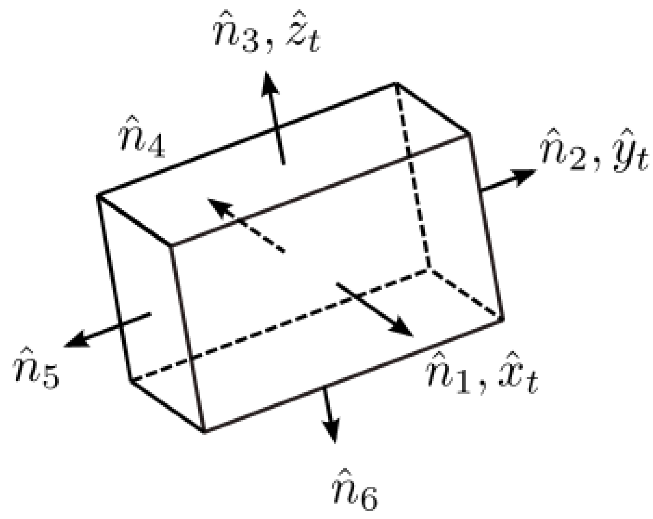
To keep the chaser from colliding with the target, the six sides of the target are used as linear constraint planes. Depending on the current position of the chaser, one of the sides is selected as the constraint. Since the normal vectors of the six sides (, ) are the principal axes of the target (see Figure 2), projecting the position vector of the chaser onto the target and selecting the plane with the vector of the largest magnitude will guarantee collision avoidance.
where the are the unit normal vectors of the sides of the target and are the distances from the center of the target to plane i plus the distances from the center of the chaser to one of its corners.
The attitude, body rates and docking port position of the target are assumed to be determined by a camera on the chaser, and the target should be within the chaser’s field of view. That is, the camera vector should always point to the target’s center of mass within a tolerance angle of alpha-FoV:
where is the camera vector fixed in the body frame, is the unit vector of the chaser position at the k-th thruster burn point, is the transformation matrix from the Hill’s frame to the body frame of the chaser, and is the half-angle field of view, as shown in Figure 1.
The thrusters’ delta-v is limited by
Additionally, Equations (14) and (15) are the constraints due to the limited torque and angular momentum storage of the chaser’s reaction wheels, respectively.
Torque constraint for each reaction wheel:
Angular momentum constraint for each reaction wheel:
In the next section, the chaser’s initial and final conditions will be derived.
3.3. Chaser’s Initial and Final Conditions
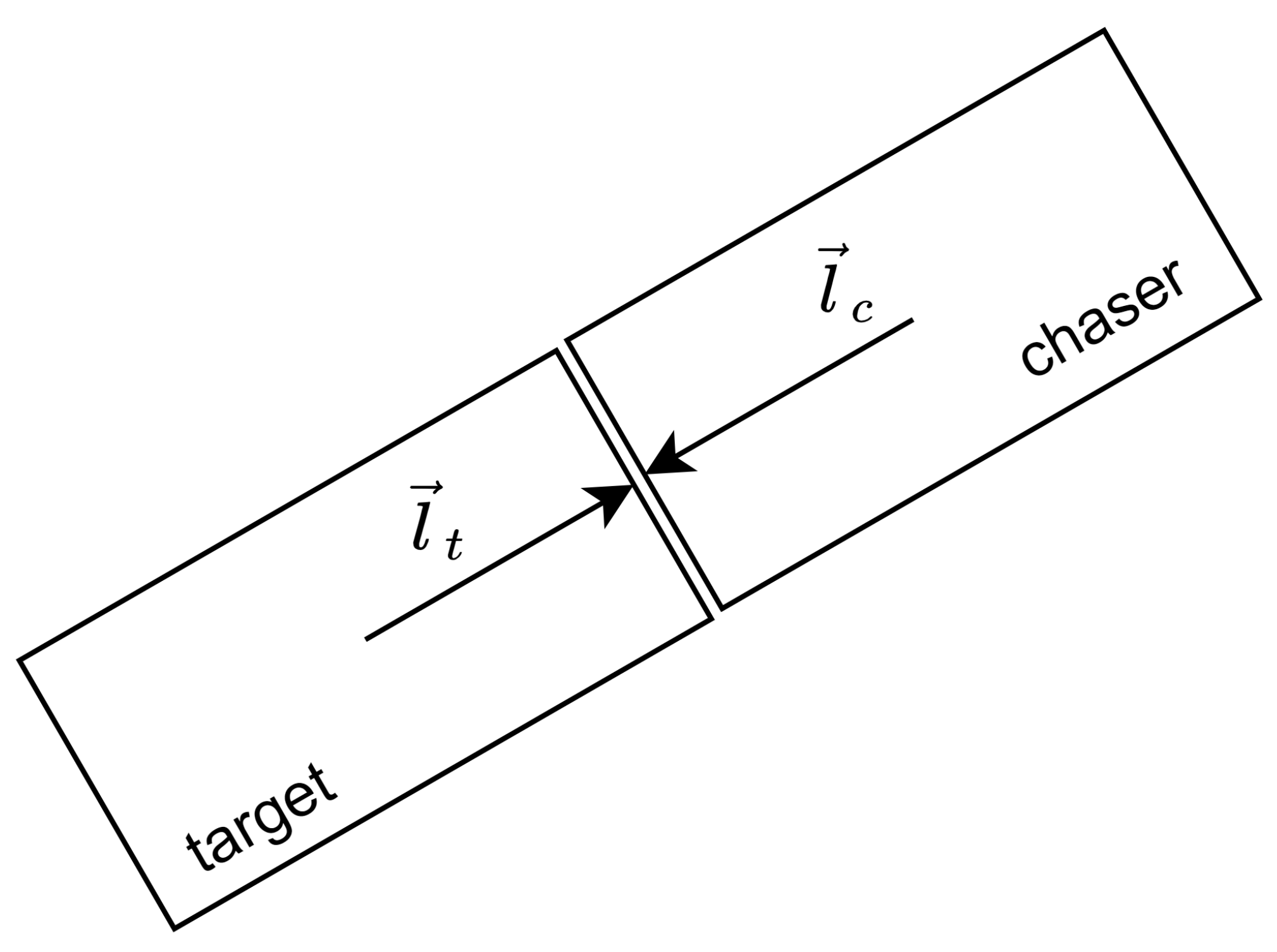
The chaser’s initial position and attitude are assumed to be known. However, the final position and attitude are determined from the target’s attitude, initial conditions and RVD duration as follows.
First, Equations (8) and (9) are numerically integrated over the duration of the RVD using the initial attitude, body rates of the target and zero input torque to obtain the target’s final attitude .
Then, the target’s docking port final position in Hill’s frame, , is obtained using Equation (16).
where is the transformation matrix of the target from the target’s body frame to Hill’s frame, which is the direction cosine matrix representation of the target’s final attitude. is the target’s docking port position in the body frame.
Finally, the chaser’s final attitude is found using the quaternion product of the required rotation quaternion between the initial and final attitude and the initial attitude quaternion .
The quaternion can be obtained from the initial and final position vectors of the chaser using Equations (19)–(21).
The initial and final constraints on the chaser states are given by
Now, the fuel optimization problem considering orbit and attitude concurrently is obtained as follows:
This coupled orbit and attitude optimization problem is nonlinear and nonconvex. Consequently, a global solution is not guaranteed, and the solution process may converge to a local minimum and require a long computation time.
By decoupling the orbit guidance problem from the attitude guidance problem and solving the attitude guidance problem analytically, the computation time can be greatly reduced because this approach leads to fewer optimization variables and constraints.
4. Decoupled Optimization Problem
For decoupling, it can be noted that the collision avoidance constraint given in Equation (11) depends solely on the position. This enables us to decouple the orbit from the attitude guidance and solve the orbit optimization without considering the attitude. In the decoupled optimization problem, first, the orbit optimization will be solved, and then an optimal attitude will be found. Since the attitude is not yet known during the orbit optimization, a fuel minimizing objective function cannot be used; instead, energy minimization will be used as the basis for the objective function, as in Equation (10). Unlike Equation (10), this objective function minimizes the delta-v in the Hill’s frame instead of in the body frame, independent of the attitude.
The constraints for the orbit optimization guidance problem are the orbit dynamics, Equation (7); the collision avoidance constraints, Equation (11); the thruster delta-v limits, Equation (13); and the initial and final constraints on the chaser position and velocity, Equation (22).
After the optimal delta-v, position and velocity of the chaser at equal time intervals have been obtained through orbit optimization, an optimal attitude can be found that minimizes the required fuel. In this case, a minimum-fuel objective function can be used, as in Equation (10), which is subjected to the attitude dynamics and field-of-view constraints at each thruster burn position.
Equations (25) and (26) are nonconvex. In the next section, Equation (25) will be convexified, and an alternative analytical solution method will be proposed for Equation (26).
4.1. Orbit Optimization
The orbit optimization problem in Equation (25) has nonlinear and nonconvex constraints. To solve this problem with a convex optimization solver, the constraints need to be convexified.
Regarding the delta-v bounds, since the attitude is not known at this moment, the required delta-v in the body frame cannot be found. Instead, the bounds on the total delta-v are established such that the total delta-v can be fired by a single thruster, which is equal to the maximum delta-v of one thruster.
4.2. Attitude Optimization
From the previous calculations, the orbit and the thrusts are already known; now, we attempt to find the attitude of the chaser at each thruster burn position, such that the fuel consumption becomes minimal.
Equation (26) gives an attitude that minimizes the required thruster burn for all thrusters. However, Equation (26) is a nonlinear optimization problem that requires considerable time to solve, and a global solution may not be found. Instead, an equivalent problem can be formulated and solved analytically to find the chaser’s attitude that minimizes the fuel without dealing with the attitude dynamics. Then, a conventional PD control method can be used to drive the chaser’s attitude to the new attitude.
The objective function in Equation (26) can be reduced to unit vector first norm optimization:
since , the objective function reduces to:
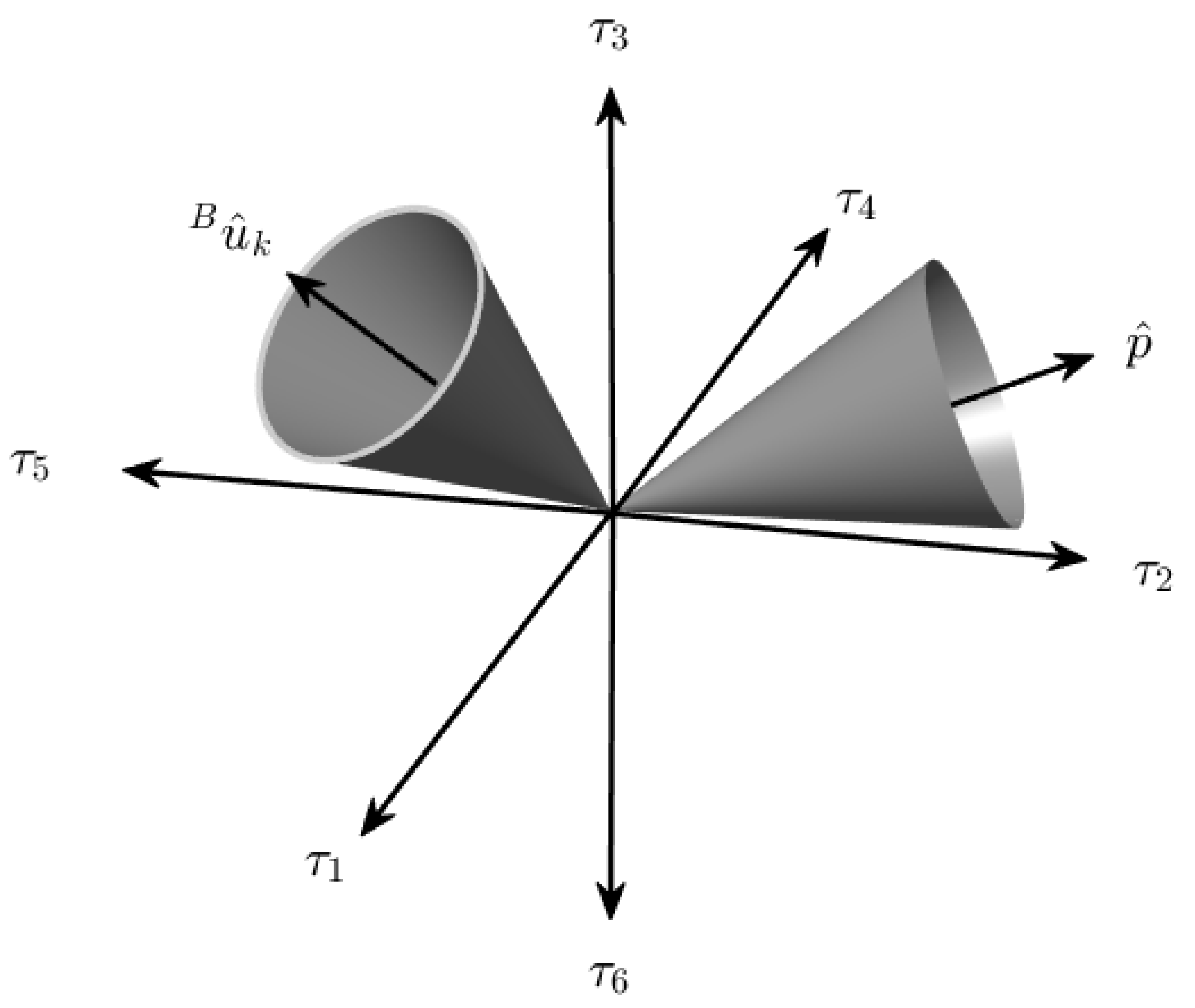
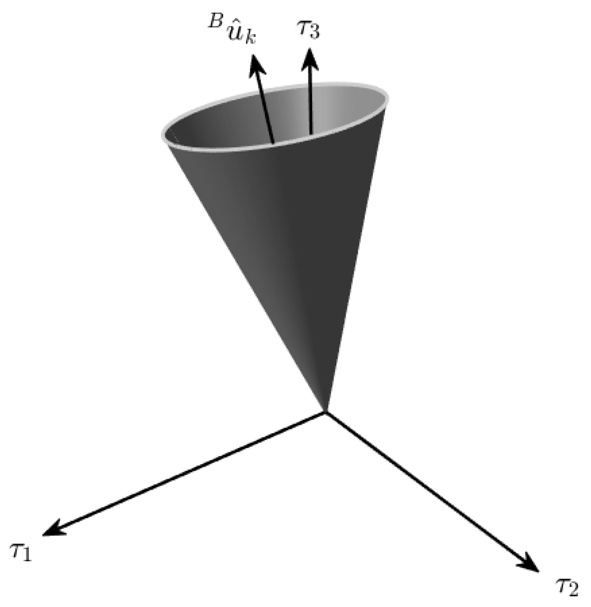
Consider that, once the orbit maneuver has been performed, the chaser has reached thruster burn position k, and the camera vector points directly to the target’s center of mass. In this case, the target is inside the field-of-view delta-v cone; hence, the field-of-view constraint is satisfied. Now, the chaser can rotate about any axis normal to the camera vector without violating the field-of-view constraint, and the required delta-v can be applied within the delta-v cone, as shown in Figure 4.
The attitude problem is now divided into two attitude maneuvers. First, an attitude is found such that the chaser points directly to the target, and then an eigen-axis rotation of or less about an axis orthogonal to the camera vector is generated.
To ensure smooth motion, the first maneuver is interpolated from the initial attitude to the docking attitude for each thruster burn position and updated in each iteration. For the second maneuver, the geometry of the chaser will be exploited to find an analytical solution.
Depending on the direction of the required delta-v vector, the delta-v cone may correspond to any of the following cases, each of which can be solved separately:
- Case 1: A thruster lies inside the delta-v cone.
- Case 2: The delta-v cone does not include a thruster and does not touch any plane formed by any two orthogonal thrusters.
- Case 3: The delta-v cone intersects with a plane formed by two orthogonal thrusters.
4.2.1. Case 1
A vector’s magnitude is always less than or equal to its first norm. This indicates that if a delta-v can be applied with a single thruster, then this will take less fuel than a thruster burn involving two or more thrusters.
In this case, as seen in Figure 5, one of the thrusters is within the delta-v cone; therefore, it is possible to move about an axis by up to without violating the field-of-view constraint such that the required delta-v burn can be applied with a single thruster.
The required attitude change can be found from the rotation axis and rotation angle calculated from the nearest thruster vector and the required delta-v in the body frame:
Rotation axis:
Rotation angle:
where is the nearest thruster vector.
To check if the required delta-v can be applied by one thruster, we can check if one of the following equations is true:
4.2.2. Case 2
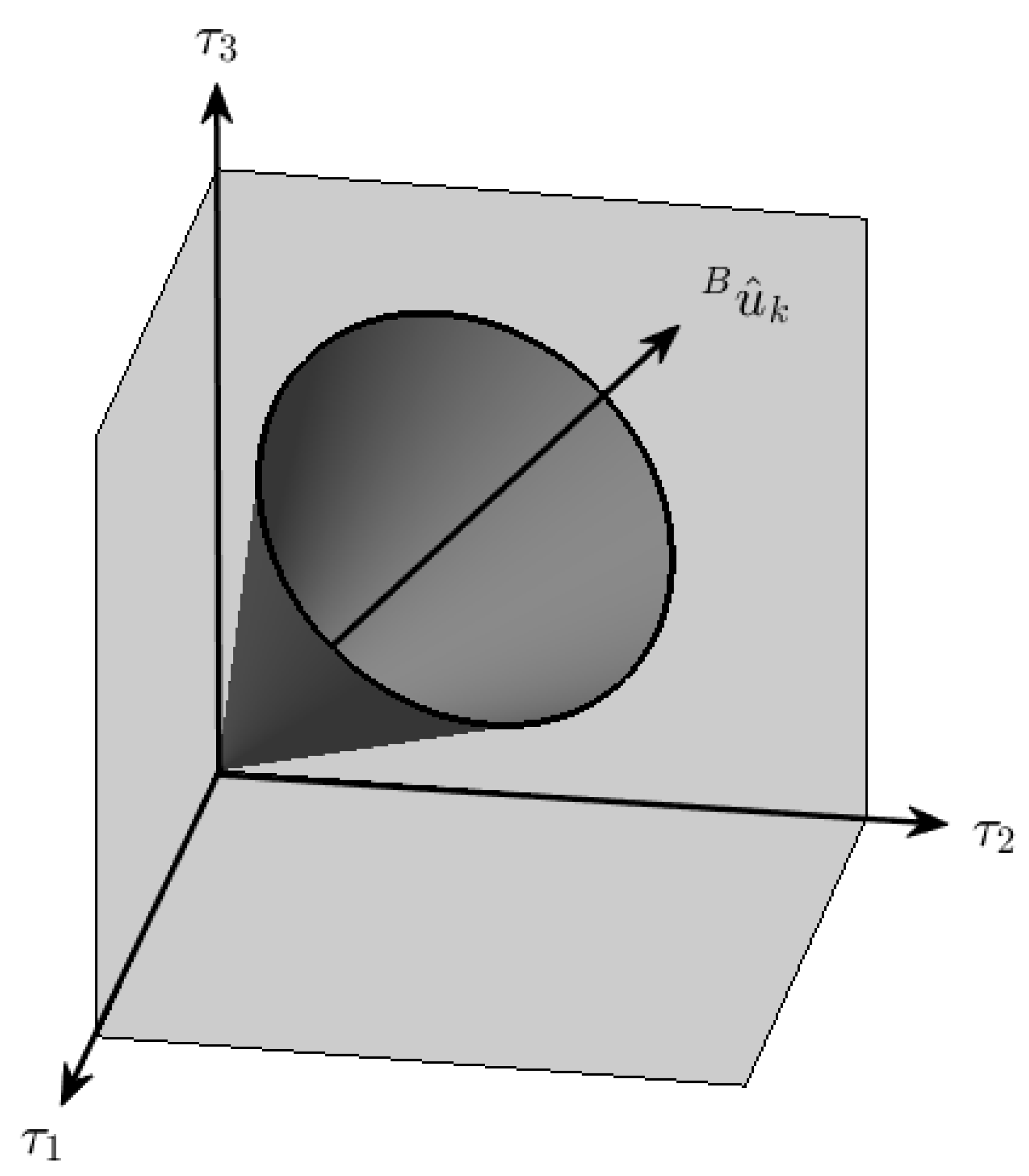
In this case, the delta-v cone around delta-v does not include any thruster within it, and it does not intersect with any plane. Therefore, the delta-v cone is suspended in a quadrant bounded by three thrusters, as shown in Figure 6.
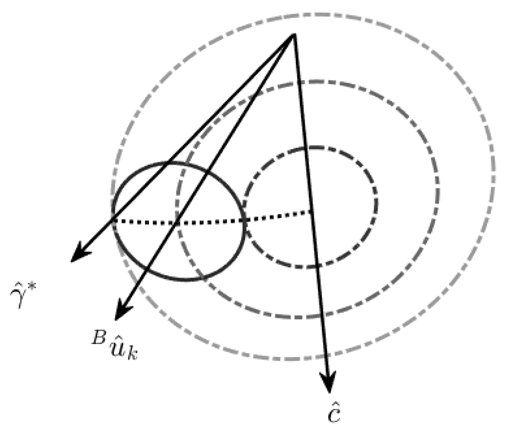
First, we will show that the optimal position of delta-v in the delta-v cone is on its edge, and then we will find the optimal unit position vector on the edge of the delta-v cone. The set of all allowed thruster burn directions is given by
where is a unit vector along the initial delta-v vector, is any unit vector orthogonal to , is a parameter that varies from 0 to , and t is a parameter that varies from 0 to . can be expressed in terms of as follows:
The first norm of is
If such that has equal components, then Equation (37) will be independent of the parameter t, which means that circles centered at have equal first norms at all their points.
Additionally, note that as decreases, the first norm increases, which indicates that the minimum of is at the edge of a circle.
Now, for a nontouching delta-v cone with a center vector at any point, we can obtain its minimum value () by solving for its intersection with a circle centered at the vector (see Figure 7).
From the geometry in Figure 7, the equations for the rotation vector and rotation axis are found as follows.
Rotation axis:
Rotation angle:
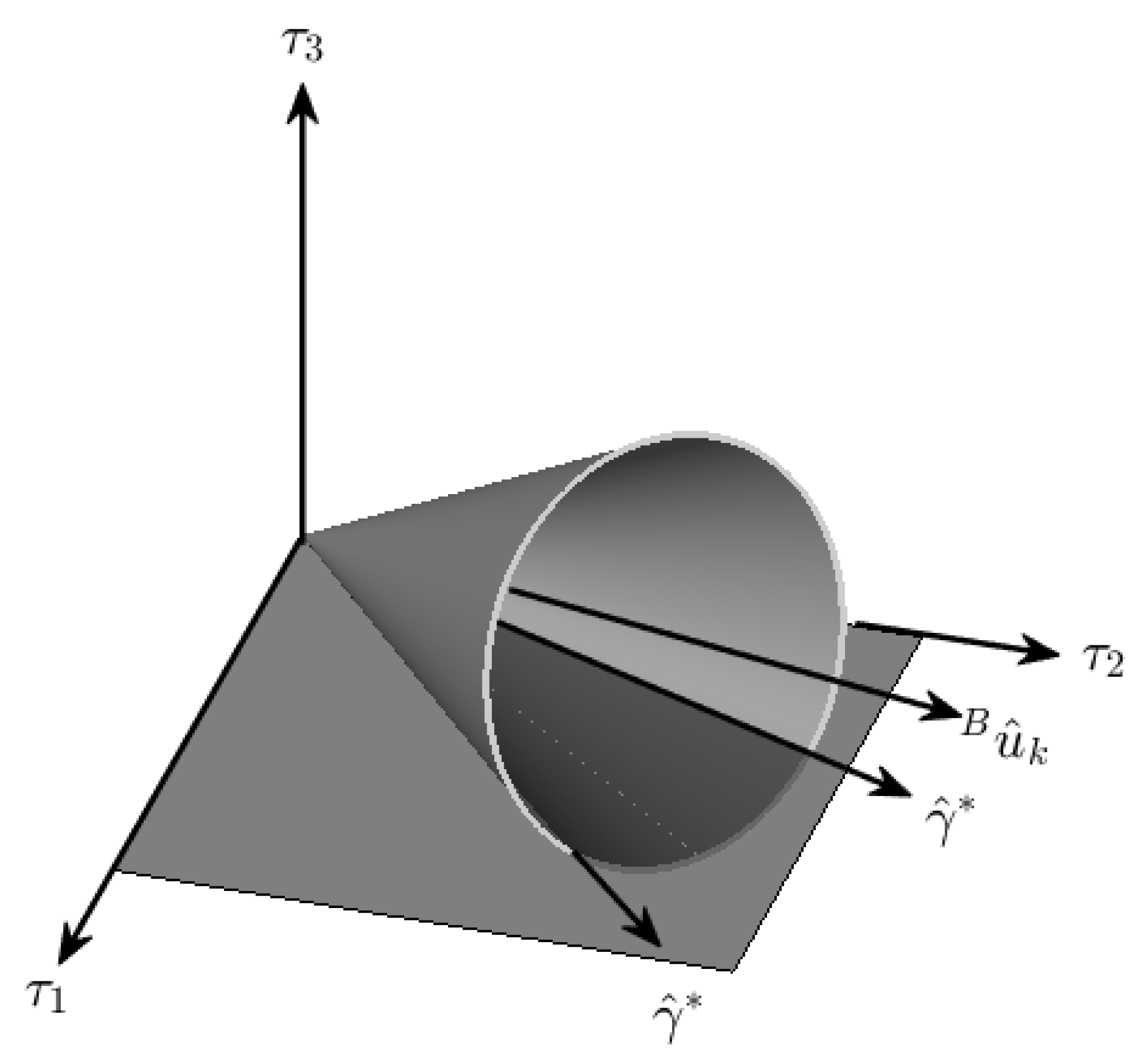
4.2.3. Case 3
When the delta-v cone intersects with a plane formed by two thrusters, as shown in Figure 8, a thruster burn can be applied anywhere on the plane between the intersection points of the delta-v cone and the plane. However, the minimum lies on the edges of the intersections.
To find the intersections, Equation (35) can be solved by setting the component along the axis normal to the plane, solving for the parameter t, and finally substituting t to obtain the components of the thrust vector. The minimum lies on either of the two intersections of the edge of the delta-v cone with the x–y plane, which are found as follows:
Similarly, intersections with the y–z and z–x planes can be found, as shown in Equation (41) and Equation (42), respectively,
In Equations (40)–(42), the terms under the square roots are used to determine whether there is an intersection with any plane. If Equation (43) is satisfied, then there is an intersection.
Rotation axis:
Rotation angle:
The minimum may also lie on the edge of a circle outside the intersection with the plane. Therefore, when the delta-v cone intersects with a plane, both case 2 and case 3 will be evaluated, and the minimum will be used.
In some cases, the delta-v cone may intersect with two planes; in such a case, the minimum among the intersections will be used.
Note that the attitude optimization does not consider the attitude dynamics and only gives the optimum orientation. Therefore, a proper control algorithm should be used to stir the spacecraft’s attitude to the one found using this algorithm. In this research, a proper PD control is assumed to be used.
The overall guidance optimization algorithm is summarized in the following section.
4.3. Guidance Optimization Algorithm
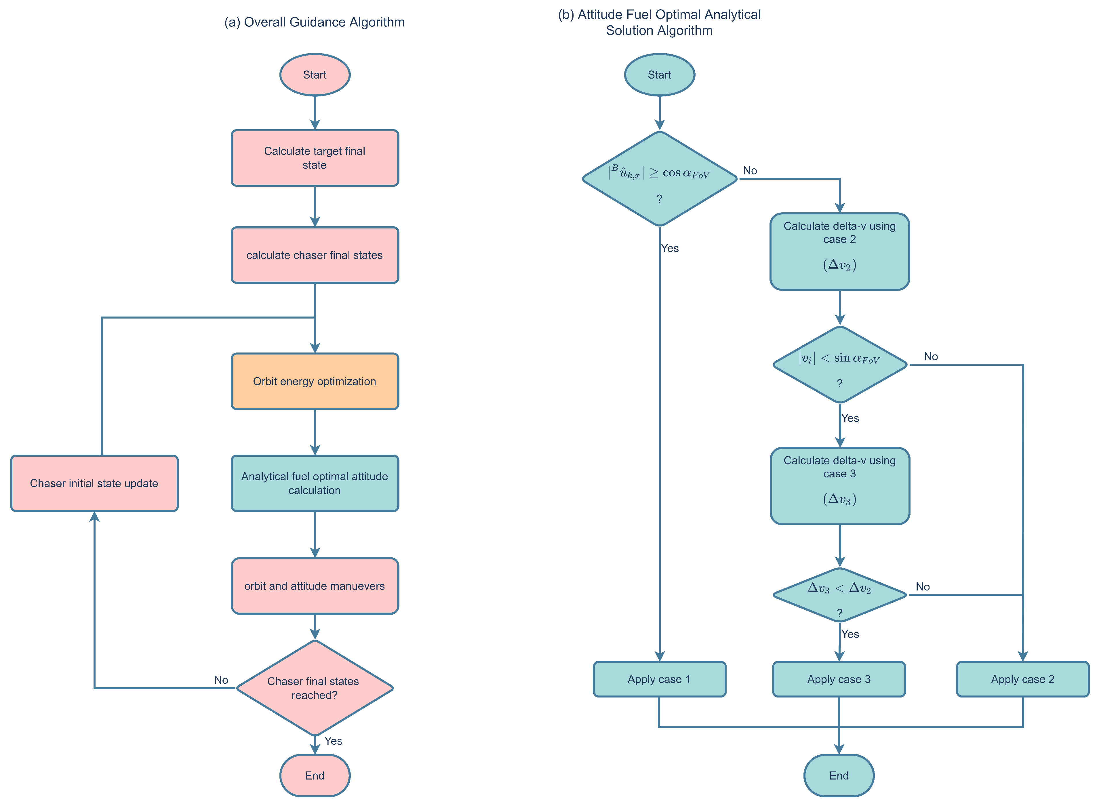
The overall guidance optimization algorithm can be summarized by the flowcharts shown in Figure 9.
The guidance algorithm is executed in the following order:
- Using the target’s initial attitude and body rates, its final attitude is obtained by integrating its dynamics and kinematics equations of motion.
- The chaser’s final position is determined from the target’s final attitude by matching the docking ports.
- Using the initial and final conditions, an energy-minimizing orbit trajectory is generated without considering safe distance constraints.
- The position at each thruster burn interval is used to linearize the safe distance constraints.
- Using the initial and final conditions, an energy-minimizing orbit trajectory is generated while considering the safe distance constraints.
- For the first thruster burn point, a fuel-optimal attitude is solved analytically by considering the field-of-view constraint.
- Attitude and orbit maneuvers are performed at the first thruster burn interval. Then, the current state is used as the initial state, the current position trajectory is used to linearize the next trajectory, and step (2) is performed until the N-th interval has been completed.
The fuel-optimal attitude analytical solution case selection is summarized as follows. First, if any of Equations (32)–(34) is satisfied, then case 1 is selected; otherwise, if Equation (43) is satisfied, then the minimum of case 2 and case 3 is selected; otherwise, case 2 is selected to obtain the optimum attitude of the chaser.
5. Simulation Results
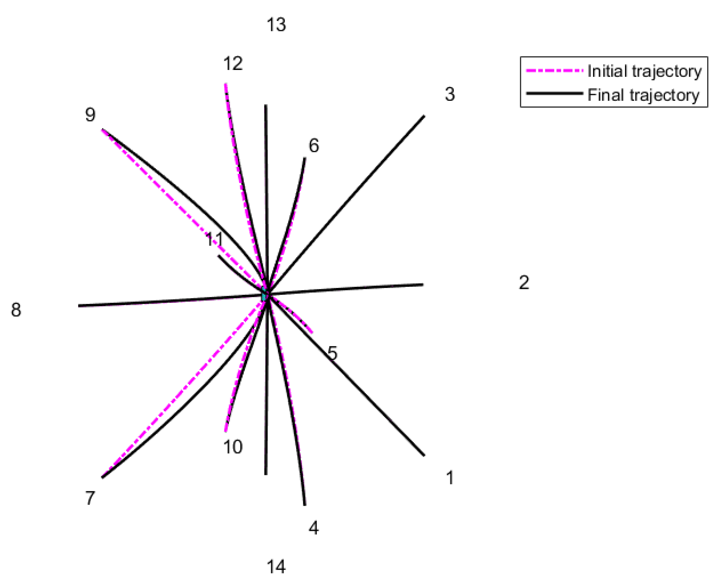
To demonstrate the performance of the proposed method, the chaser was initialized at 14 different positions in space, as shown in Figure 10, with the parameters given in Table 1. The starting distance at all positions was 10 m, and the starting attitude was such that the camera vector was pointing directly to the target.
All simulations were carried out in MATLAB 2021a on a computer with a Core i7 processor and 8 GB of RAM.
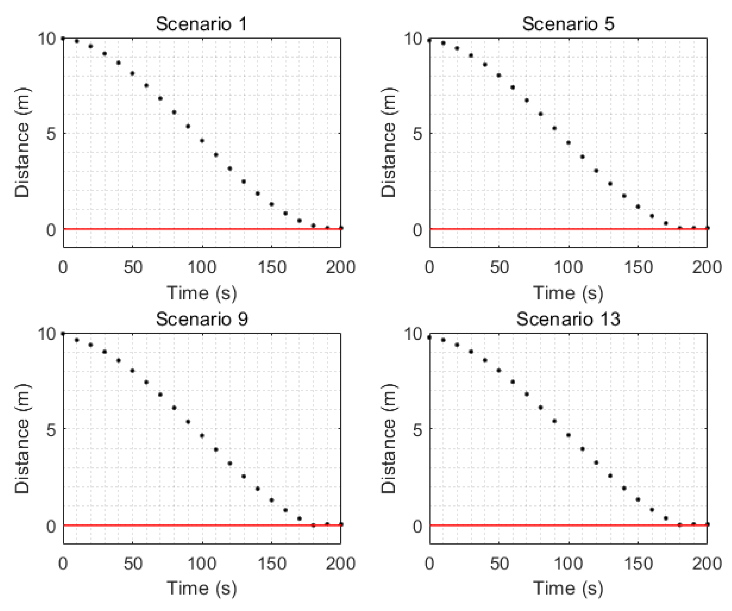
In Figure 10, the starting positions are marked with their respective numbers. The dashed lines are the paths followed without safe distance constraints, while the solid lines are the final trajectories with all constraints considered. In some scenarios, the initial trajectory crosses the safe distance, but once the safe distance constraints are included, a safe distance is maintained. In all test cases, docking to the target is successfully achieved, and no collision with the target occurs, as shown in Figure 11; only four scenarios are shown for convenience.
Figure 12 presents a fuel usage comparison between the proposed method and the same method but without attitude optimization, using only quaternion feedback to align the chaser camera to the target. The fuel usage decreases from a delta-v of 0.200 m/s to a delta-v of 0.175 m/s, which is a 12.5% saving.
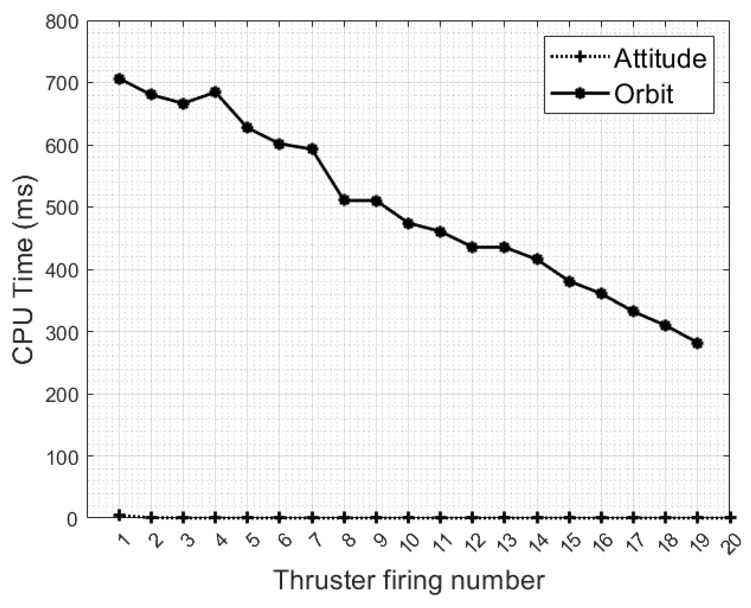
For the same scenario, Figure 13 shows the computation times for orbit optimization and attitude optimization. Orbit optimization takes from approximately 700 ms at the start of the trajectory to 280 ms near docking, while attitude optimization consumes less than 10 ms of processor time.
6. Conclusions
This paper studies the fuel consumption and computation time for the autonomous RVD of a spacecraft with a target. The nonlinear and nonconvex constrained optimization problem is formulated by considering the nonlinear dynamics of the chaser model in the Hill’s frame and various coupling constraints between orbit and attitude guidance. Then, we propose a novel method of decoupling the optimization problem into two subproblems of orbit optimization and attitude optimization. Next, we convert the orbit optimization subproblem into a convex optimization problem and solve it using a conventional convex optimization solver. Finally, the attitude optimization subproblem is efficiently solved analytically by exploiting the attitude geometry. By virtue of this analytical solution, on-board computation and implementation is made possible through the proposed approach. Fourteen scenarios are considered to validate the effectiveness and computational efficiency of our proposed approach. In all scenarios, the computation time is greatly reduced and the fuel is saved up to 12.5%, due to the use of an analytical method for attitude optimization.
Author Contributions
Conceptualization, A.M.O. and D.-K.K.; methodology, A.M.O. and D.-K.K.; software, A.M.O.; validation, A.M.O.; formal analysis, A.M.O.; investigation, A.M.O. and D.-K.K.; resources, A.M.O.; data curation, A.M.O.; writing—original draft preparation, A.M.O.; writing—review and editing, A.M.O. and D.-K.K.; visualization, A.M.O.; supervision, D.-K.K.; project administration, A.M.O.; funding acquisition, D.-K.K. All authors have read and agreed to the published version of the manuscript.
Funding
This work was supported by the KARI (under a contract with the Ministry of Science and ICT) through the “Development of Pathfinder Lunar Orbiter and Key Technologies for the Second Stage Lunar Exploration” project (2016M1A3A9005561).
Institutional Review Board Statement
Not applicable.
Informed Consent Statement
Not applicable.
Data Availability Statement
The data presented in this study are available on request from the corresponding author.
Conflicts of Interest
The authors declare no conflict of interest.
Abbreviations
The following abbreviations are used in this manuscript:
| RVD | Rendezvous and docking |
| MPC | Model predictive control |
| LQC | Linear quadratic control |
| LEO | Low Earth orbit |
| STM | State transition matrix |
References
- Boyarko, G.; Yakimenko, O.; Romano, M. Optimal rendezvous trajectories of a controlled spacecraft and a tumbling object. J. Guid. Control Dyn. 2011, 34, 1239–1252. [Google Scholar] [CrossRef]
- Ventura, J. Fast and Near-Optimal Guidance for Docking to Uncontrolled Spacecraft. J. Guid. Control Dyn. 2017, 40, 3138–3154. [Google Scholar] [CrossRef]
- Sanchez, J.C.; Gavilan, F.; Vazquez, R.; Louembet, C. A flatness-based predictive controller for six-degrees of freedom spacecraft rendezvous. Acta Astronaut. 2020, 167, 391–403. [Google Scholar] [CrossRef] [Green Version]
- Hu, Q.; Xie, J.; Liu, X. Trajectory optimization for accompanying satellite obstacle avoidance. Aerosp. Sci. Technol. 2018, 82–83, 220–233. [Google Scholar] [CrossRef]
- Murtazin, R.; Sevastiyanov, N.; Chudinov, N. Fast rendezvous profile evolution: From ISS to lunar station. Acta Astronaut. 2020, 173, 139–144. [Google Scholar] [CrossRef]
- Breger, L.; How, J.P. Safe trajectories for autonomous rendezvous of spacecraft. J. Guid. Control Dyn. 2008, 31, 1478–1489. [Google Scholar] [CrossRef]
- Li, Q.; Yuan, J.; Zhang, B.; Gao, C. Model predictive control for autonomous rendezvous and docking with a tumbling target. Aerosp. Sci. Technol. 2017, 69, 700–711. [Google Scholar] [CrossRef]
- Zagaris, C.; Park, H.; Virgili-Llop, J.; Zappulla, R.; Romano, M.; Kolmanovsky, I. Model predictive control of spacecraft relative motion with convexified keep-out-zone constraints. J. Guid. Control Dyn. 2018, 41, 2054–2062. [Google Scholar] [CrossRef]
- Lu, P.; Liu, X. Autonomous trajectory planning for rendezvous and proximity operations by conic optimization. J. Guid. Control Dyn. 2013, 36, 375–389. [Google Scholar] [CrossRef]
- Moon, G.H.; Lee, B.Y.; Tahk, M.J.; Shim, D.H. Quaternion based attitude control and suboptimal rendezvous guidance on satellite proximity operation. In Proceedings of the 2016 European Control Conference, ECC 2016, Aalborg, Denmark, 29 June–1 July 2016. [Google Scholar] [CrossRef]
- Wu, Y.; Cao, X.; Xing, Y.; Zheng, P.; Zhang, S. Relative motion decoupled control for spacecraft formation with coupled translational and rotational dynamics. In Proceedings of the 2009 International Conference on Computer Modeling and Simulation, ICCMS 2009, Macau, China, 20–22 February 2009. [Google Scholar] [CrossRef]
- Zappulla, R.; Park, H.; Virgili-Llop, J.; Romano, M. Real-Time Autonomous Spacecraft Proximity Maneuvers and Docking Using an Adaptive Artificial Potential Field Approach. IEEE Trans. Control Syst. Technol. 2019, 27, 2598–2605. [Google Scholar] [CrossRef]
- Samsam, S.; Chhabra, R. Multi-impulse Shape-based Trajectory Optimization for Target Chasing in On-orbit Servicing Missions. In Proceedings of the 2021 IEEE Aerospace Conference (50100), Big Sky, MT, USA, 6–13 March 2021; IEEE: Piscataway, NJ, USA, 2021; pp. 1–11. [Google Scholar] [CrossRef]
- Di Cairano, S.; Park, H.; Kolmanovsky, I. Model predictive control approach for guidance of spacecraft rendezvous and proximity maneuvering. Int. J. Robust Nonlinear Control 2012, 22, 1398–1427. [Google Scholar] [CrossRef] [Green Version]
- Sidi, M.J. Spacecraft Dynamics and Control: A Practical Engineering Approach; Cambridge Aerospace Series; Cambridge University Press: Cambridge, UK, 1997. [Google Scholar] [CrossRef]
- Melton, R.G. Time-explicit representation of relative motion between elliptical orbits. J. Guid. Control Dyn. 2000, 23, 604–610. [Google Scholar] [CrossRef]
- Shuster, M.D. Survey of attitude representations. J. Astronaut. Sci. 1993, 41, 439–517. [Google Scholar]
- Andersen, E.D.; Andersen, K.D. The Mosek Interior Point Optimizer for Linear Programming: An Implementation of the Homogeneous Algorithm. In High Performance Optimization; Springer: Boston, MA, USA, 2000; pp. 197–232. [Google Scholar] [CrossRef]
- Sturm, J.F. Using SeDuMi 1.02, a MATLAB toolbox for optimization over symmetric cones. Optim. Methods Softw. 1999, 11, 625–653. [Google Scholar] [CrossRef]
- Toh, K.; Tütüncü, R.; Todd, M. SDPT3—A Matlab software package for semidefinite-quadratic-linear programming. Optim. Methods Softw. 1999, 11, 545–581. [Google Scholar] [CrossRef]
- Grant, M.; Boyd, S. CVX: Matlab Software for Disciplined Convex Programming, Version 2.1. 2014. Available online: http://cvxr.com/cvx (accessed on 14 June 2021).
Figure 1.
RVD geometry and coordinate frames.

Figure 2.
The six sides of the target are the limits preventing the chaser from colliding with the target.
Figure 2.
The six sides of the target are the limits preventing the chaser from colliding with the target.

Figure 3.
Final docking configuration where the chaser’s docking port matches the target’s docking port and the chaser’s final position and attitude are determined from the target’s final attitude.
Figure 3.
Final docking configuration where the chaser’s docking port matches the target’s docking port and the chaser’s final position and attitude are determined from the target’s final attitude.

Figure 4.
Attitude optimization configuration: field-of-view cone centered at and delta-v cone centered at , at an attitude where points directly to the target.
Figure 4.
Attitude optimization configuration: field-of-view cone centered at and delta-v cone centered at , at an attitude where points directly to the target.

Figure 5.
Case 1: a thruster inside the delta-v cone.

Figure 6.
Case 2: the delta-v cone does not intersect with any plane and does not include any thruster.
Figure 6.
Case 2: the delta-v cone does not intersect with any plane and does not include any thruster.

Figure 7.
Geometry for case 2: all components of the vector are equal, and reaches its minimum at the intersection of the circle and the farthest circle around , that is at .
Figure 7.
Geometry for case 2: all components of the vector are equal, and reaches its minimum at the intersection of the circle and the farthest circle around , that is at .

Figure 8.
Case 3: the delta-v cone intersects with -, and the optimal firing directions are along either of the vectors.
Figure 8.
Case 3: the delta-v cone intersects with -, and the optimal firing directions are along either of the vectors.

Figure 9.
Guidance algorithm flowchart.

Figure 10.
3D view of trajectories started at 14 different positions in space.

Figure 11.
Safe distance limit: the dashed line is the safety limit, and a negative value indicates collision of four scenarios.
Figure 11.
Safe distance limit: the dashed line is the safety limit, and a negative value indicates collision of four scenarios.

Figure 12.
Fuel usage comparison.

Figure 13.
Computation time comparison.


Table 1.
Chaser and target parameters.
| Parameter | Unit | Value |
|---|---|---|
| chaser and target dimensions | m | [5, 10, 15]’ |
| chaser docking port | [1, 0, 0]’ | |
| target docking port | [1, 0, 0]’ | |
| camera vector | [1, 0, 0]’ | |
| initial body rate of target | rad/s | [1.5, 1.5, 1.5]’ |
| initial body rate of chaser | rad/s | [0, 0, 0]’ |
| initial velocity of chaser | m/s | [0, 0, 0]’ |
| initial attitude of chaser | [1, 0, 0, 0]’ | |
| initial attitude of target | [0.5, 0.5, 0.5, 0.5]’ | |
| half-angle field of view | degrees | 20 |
| maximum delta-v | m/s | 0.37 |
| duration | seconds | 200 |
| number of thruster burns | 20 | |
| mass of target | kg | 6 |
| moment of inertia of target | kg·m2 | |
| mass of chaser | kg | 6 |
| moment of inertia of chaser | kg·m2 | |
| altitude | km | 400 |
| reaction wheel maximum torque | mNm | 2.3 |
| reaction wheel momentum storage | mNms | 30.0 |
Publisher’s Note: MDPI stays neutral with regard to jurisdictional claims in published maps and institutional affiliations. |
© 2022 by the authors. Licensee MDPI, Basel, Switzerland. This article is an open access article distributed under the terms and conditions of the Creative Commons Attribution (CC BY) license (https://creativecommons.org/licenses/by/4.0/).
Share and Cite
MDPI and ACS Style
Oumer, A.M.; Kim, D.-K. Real-Time Fuel Optimization and Guidance for Spacecraft Rendezvous and Docking. Aerospace 2022, 9, 276. https://0-doi-org.brum.beds.ac.uk/10.3390/aerospace9050276
AMA Style
Oumer AM, Kim D-K. Real-Time Fuel Optimization and Guidance for Spacecraft Rendezvous and Docking. Aerospace. 2022; 9(5):276. https://0-doi-org.brum.beds.ac.uk/10.3390/aerospace9050276
Chicago/Turabian StyleOumer, Ahmed Mehamed, and Dae-Kwan Kim. 2022. "Real-Time Fuel Optimization and Guidance for Spacecraft Rendezvous and Docking" Aerospace 9, no. 5: 276. https://0-doi-org.brum.beds.ac.uk/10.3390/aerospace9050276
Note that from the first issue of 2016, this journal uses article numbers instead of page numbers. See further details here.