Article

Water Surface Flight Control of a Cross Domain Robot Based on an Adaptive and Robust Sliding Mode Barrier Control Algorithm

1
School of Computer Science and Engineering, Nanjing University of Science and Technology, Nanjing 210018, China
2
School of Mechanical Engineering, Nanjing University of Science and Technology, Nanjing 210018, China
*
Author to whom correspondence should be addressed.
Submission received: 8 May 2022 / Revised: 15 June 2022 / Accepted: 17 June 2022 / Published: 21 June 2022
(This article belongs to the Special Issue Applications of Drones)

Abstract

:
When a cross-domain robot (CDR) flies on the water surface, the large pitch angle and roll angle may lead to water flooding into the robot cabin or even overturning. In addition, the CDR is influenced by some uncertain parameters and external disturbances, such as the water resistance and current. To constrain the robot attitude angle and improve the robustness of the controller, a non-singular terminal sliding mode asymmetric barrier control (NTSMABC) algorithm is proposed. All the uncertain disturbances are regarded as a lump disturbance, and a radial basis function neural network (RBFNN) is designed to compensate for the output of the controllers. Unlike the traditional quadrotors, the robot controls the yaw angle by paddles when the robot flies on the water surface. To prevent the actuator saturation and the robot from rolling over due to excessive yaw angular velocity, an adaptive integral sliding mode barrier control (AISMBC) algorithm is proposed to constrain the yaw angular velocity directly. This algorithm adaptively adjusts the gain of the sliding surface to suppress the influence of the lump disturbance on the robot. Another RBFNN is designed to compensate for the output of the controller. Simulation results demonstrate the effectiveness of the proposed control methods.

1. Introduction

Rotorcrafts, wheeled mobile robots (WMRs), and unmanned surface vehicles (USVs) have been studied for serval years, but these robots can only work in a single environment [1]. To overcome the shortages of the traditional robots, multi-habitat robots have been rapidly developed. Spherical robots are one of the popular structures [2,3]. The quadrotor is enclosed in a spherical shell; therefore, the robot can work in three environments [4]. A leg-type amphibious robot was presented in [5], which can move on the ground with its legs, and generates traction by spraying water on the water surface. More interesting robots can be found in [6,7,8]. The micro aerial vehicles (MAVs) equipped with optical flow sensors can realize obstacle avoidance, measurement distance, and velocity estimation. In [9], two optical flow sensors constituted an optical flow divergence which was placed on an MAV to avoid obstacles. This method improved the success rate of obstacle avoidance. In [10], the optical flow sensor was used to estimate the velocity of MAV, and a stereo camera with a mass of 4 g was adapted for visual navigation. The autonomous obstacle avoidance of this pocket MAV was realized in indoor environments.
The research about CDRs and amphibious robots has mainly focused on structural innovations, while the research has paid less attention to robot control methods. In this paper, we focus on the control algorithms of the CDRs flying on the water surface. There is some research on control algorithms for CDRs, but the research is abundant for similar control systems such as quadrotor UAVs, WMRs, and USVs. The backstepping control is a classical control algorithm. In [11], the quadrotor UAV was controlled by the adaptive integral backstepping algorithm and an adaptive law was designed to compensate the lumped disturbance. In [12], the backstepping-based algorithm was also adopted to achieve cooperation control of multiple USVs. In addition, there are intelligent control methods, such as model predictive control (MPC) [13], reinforcement learning [14], deep reinforcement learning [15], and so on.
However, the constraints on the system states were not considered in the above control algorithms. To constrain the system states, the controllers based on the barrier Lyapunov function (BLF) [16] and the integral barrier Lyapunov function (IBLF) [17] are classical barrier control (BC) algorithms. Following the traditional idea of BC, multiple brilliant control methods have been proposed. In [18], an adaptive barrier controller was proposed for the strict feedback system. The unknown disturbances were compensated by an adaptive law. Based on integral barrier control, a time-varying constrained barrier control was proposed, but the time-varying boundary was not changed with the system state [19]. Besides, there are barrier control algorithms based on tanh-type [20]. For the specific control systems, the study introduced in [21] provided a new integral barrier controller to directly constrain the quadrotor attitude, which solved the conservative problem of the traditional integral BC. To constrain the full-states of underactuated system, such as WMRs, a finite-time barrier control algorithm was proposed [22]. Designing an adaptive law for the uncertain term of the control system is a useful method but another way is to use the observer or the neural network. In [23], a radial basis function neural network (RBFNN) was designed to approach the lumped disturbance of missile autopilot dynamic model. In [24], the RBFNN was used to obtain the lumped disturbance of USVs. Similar ideas can be found in [25,26].
To make the proposed control algorithms more robust, the sliding mode control is used as a basis of the control algorithms. Sliding mode control (SMC) has been widely studied in recent years because of its insensitivity to system parameters and strong robustness. To eliminate the static error of SMC, the integral term is introduced into sliding mode surface [27]. To speed up the convergence speed of system errors, terminal sliding mode control (TSMC) and nonsingular terminal sliding mode control (NTSMC) have been proposed. A fast terminal sliding mode algorithm is adopted to the position control and attitude control of the quadrotor. The tanh function is adopted in the sliding mode surface to further speed up the controllers, but the controller is complex [28]. A fast-nonsingular terminal sliding mode control (FNTSMC) has been proposed for autonomous underwater vehicles, and the external disturbances and disturbances caused by uncertain parameters were obtained by the observer [29]. In addition, adaptive sliding mode control (ASMC) is also a common control method to control USVs and quadrotor UAVs [30,31].
Some conventional strategies have been used in the literature to achieve a better robustness. For example, a filtered observer-based IDA-PBC was proposed in [32], which could reduce the influence caused by the sensor measure noises and the quadrotor states uncertain. In [33], a simple and robust controller was developed that had no observer or adaptive law. For the sake of better robustness and the constrains on system states, there are numerous comprehensive control algorithms that have been proposed such as the controller, which combines the NTSMC with BC, and can adaptively adjust the gain of the sliding mode, thus improving the robustness of the controller [34]. In [35], a composite time-varying tanh-type barrier Lyapunov function was designed, and the uncertainties and external disturbances in the attitude control of quadrotor were solved by the adaptive law. However, the controller is complicated. The controllers proposed in [34,35] had similar ideas in the proof of state error convergence. In [36], the ISMC was adopted and the constraints on system state were considered. The control methods combining SMC with BC can be found in [37,38]. Besides, the comprehensive control algorithms, such as combining fuzzy control with BC [39] and MPC based on barrier Lyapunov function [40] are both known as effective state-constrained control methods.
Through the discussion of the control methods above and inspired by [34,35], a nonsingular terminal sliding mode asymmetric barrier control (NTSMABC) algorithm is proposed to constrain the pitch angle and roll angle of CDR when the robot flies on the water surface. Enlightened by reference [36], an adaptive integral sliding mode barrier control (AISMBC)was applied to constrain the yaw angular velocity of the robot. The main contributions of this paper are as follows:
  • A CDR that can work in three environments is designed. The dynamic model for the CDR flying on the water surface is presented;
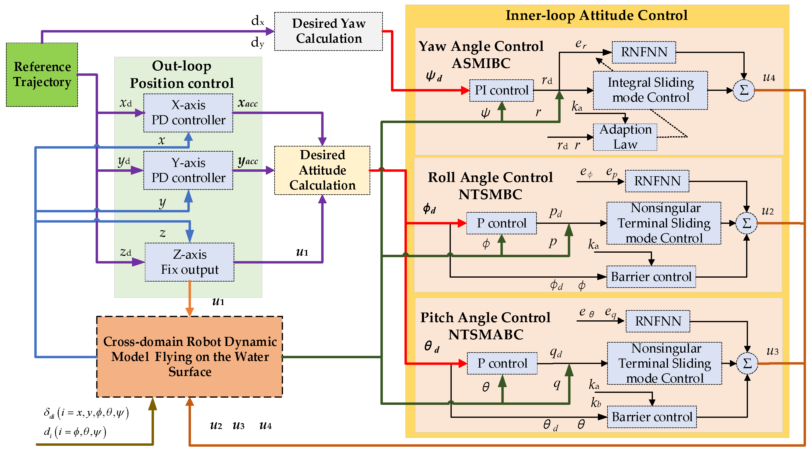
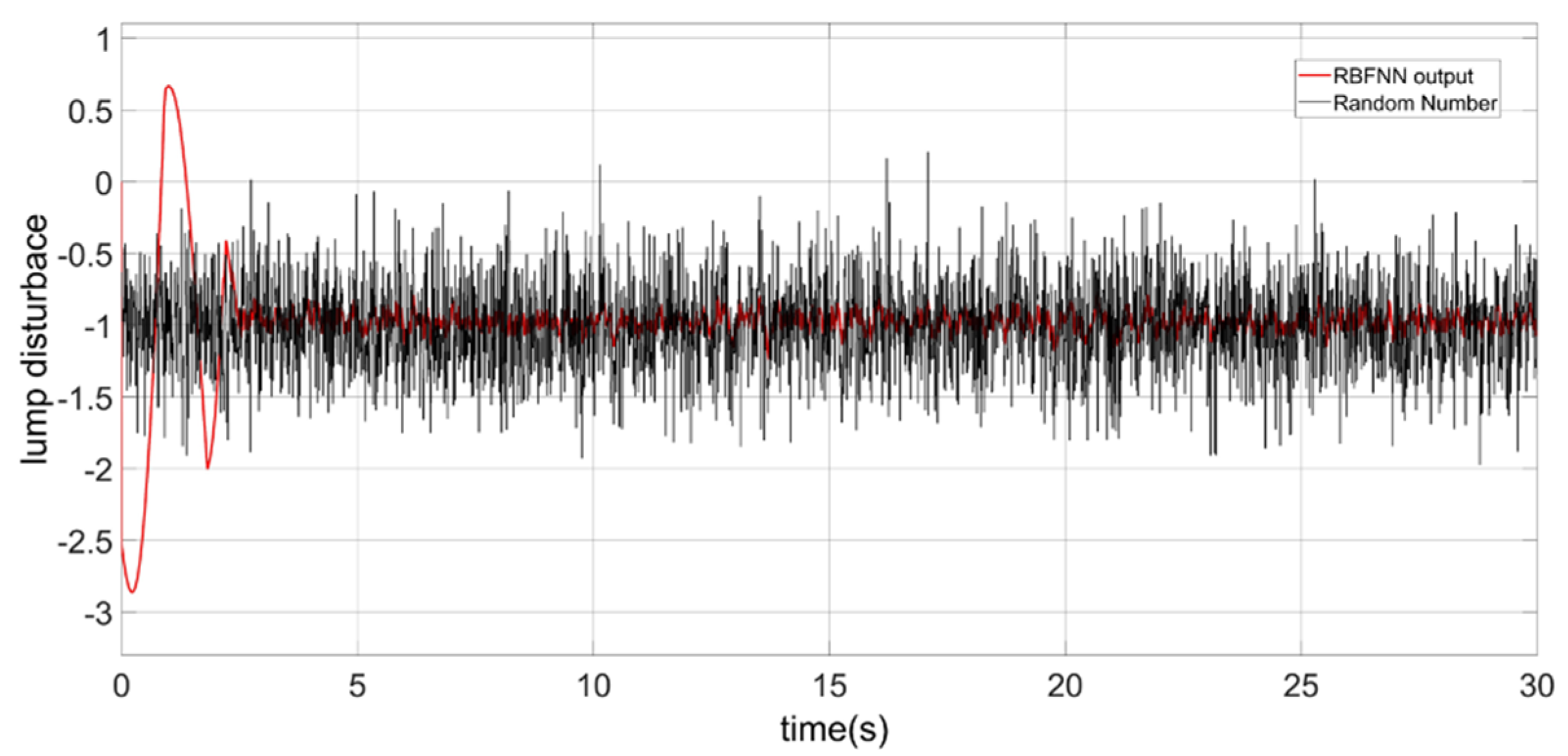
  • Based on the traditional BC [16], a nonsingular terminal sliding mode asymmetric barrier control (NTSMABC) algorithm is proposed to constrain the pitch angle and roll angle of CDR on the water surface. Since the robot has an asymmetric structure which is similar with a small USV, the roll angle is controlled by NTSMBC, but the pitch angle is controlled by NTSMABC. To handle the lumped disturbance including uncertain model parameters and time-vary external disturbances, a RBFNN is adopted to compensate for the controller. Moreover, an adaptive law of neural network weight is designed with the Lyapunov function. The proposed method combines NTSMC with BC, which improves the convergence speed of the state errors and robustness;
  • Inspired by references [35,36], an adaptive integral sliding mode barrier control (AISMBC) is proposed to constrain the yaw angular velocity. The sliding mode surface we designed only includes the angular velocity state error, and the gain of sliding mode is adaptively adjusted according to the difference between the actual state and the barrier value. RBFNN is also designed to obtain the uncertain lump disturbance. The weights of the neural network are adjusted by the adaptive rate.
This paper is organized as follows. In Section 2, preliminary works and a brief introduction of the CDR are given. In Section 3, the NTSMABC and the AISMBC are introduced, and detailed proofs of convergence are presented. The simulation results of the robot flying on the water surface are provided in Section 4 to verify the effectiveness of our control methods. Section 5 concludes our work and introduces further work.

2. Preliminary Work and the Mathematic Model

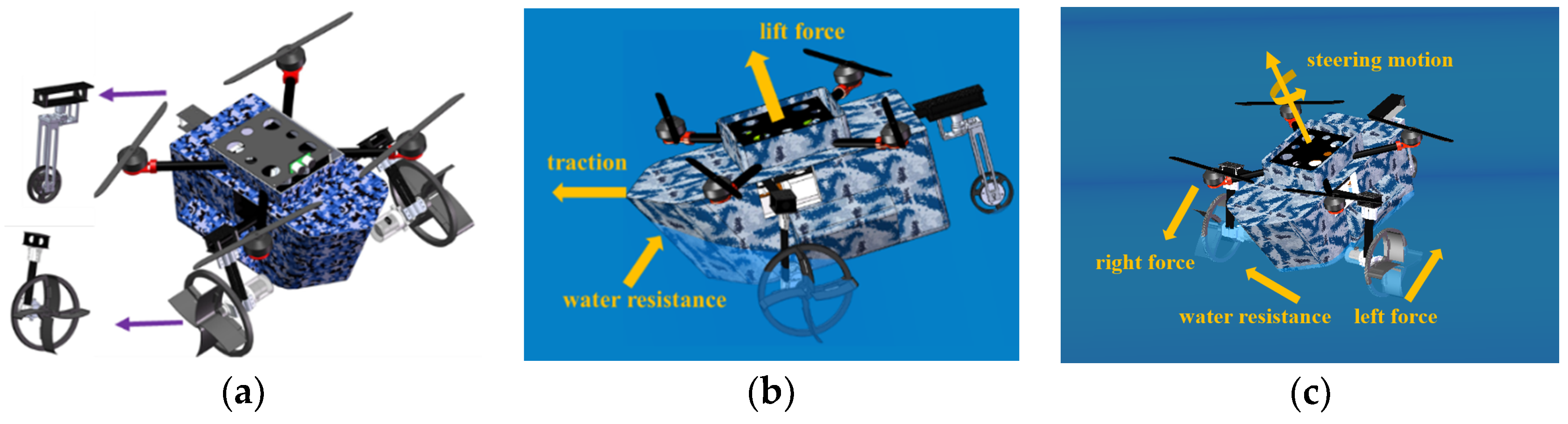
2.1. The Introduction of the Cross-Domain Robot

This part introduces the structure of the robot when flying on the water surface. The robot can be roughly considered as a combination of the WMR with the quadrotor. The structure of the CDR is shown in Figure 1.
Figure 1a shows the structure of the robot. The paddles are integrated with the wheels to give the robot extra power when moving on the water surface. The robot flying on the water surface is shown in Figure 1b. The propulsion is generated by the component of the rotor lift force. This is because the shell of the robot is similar to a boat-type. When the robot moves backward, it is subjected to greater water resistance. To ensure the safety of the robot moving on the water, the structure of the robot is not completely symmetrical. Therefore, the pitch angle of the robot is constrained asymmetrically. Besides, this constrained condition can prevent the robot from moving backward. The roll angle can be constrained symmetrically. The robot yaw angle is controlled by the paddles as shown in Figure 1c. The robot flying on the water surface is shown in Figure 2.

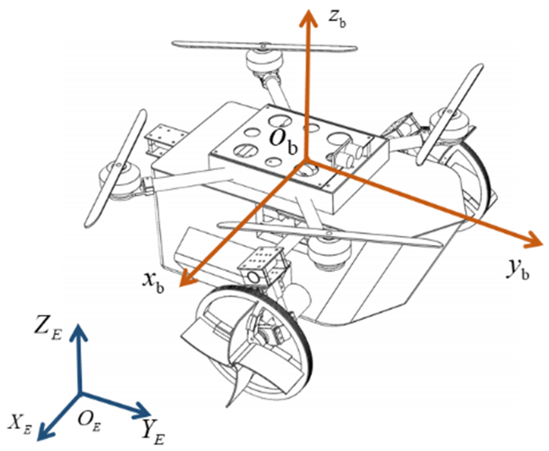
2.2. Dynamic Model of the Cross-Domain Robot

In this paper, we focus on the control algorithm of a robot flying on the water surface. Therefore, only the dynamic model of the robot flying on the water surface is shown. Some assumptions are proposed before the mathematical model of the robot moving on the water surface is established.
Assumption 1.
The robot is a rigid body, its mass distribution is homogeneous, and the shape structure is a port/starboard symmetric.
Assumption 2.
The center of gravity of the robot body coincides with the geometric center.
Assumption 3.
The total lift provided by the rotors is smaller than the gravity of the robot.
Assumption 4.
The power generated by the rotors and paddles satisfies the requirement of the robot.
Based on our previous work [41], the WMR mathematical model [25], and the mathematical model of the quadrotor [35], the dynamic model of the CDR in a coordinate frame is shown in Figure 3.
As shown in Figure 3, E ( O , X , Y , Z ) is the earth coordinate frame. b ( o , x , y , z ) is the body coordinate frame. The robot position on the water surface is defined as ξ = [ x y z ] T . The attitude angle of robot in the earth coordinate frame is defined as Φ = [ ϕ θ ψ ] T , which represents the roll angle, pitch angle, and yaw angle, respectively. The angular velocity in the body coordinate frame is defined as Ω = [ p q r ] T . When the attitude satisfies the small angle assumption, Φ ˙ = Ω . The dynamic model of the CDR on the water surface can be expressed as follows:
{ x ¨ = [ u 1 ( c ϕ s θ c ψ + s ϕ s ψ ) δ d x ( x ) ] / m y ¨ = [ u 1 ( c ϕ s θ s ψ s ϕ c ψ ) δ d y ( y ) ] / m z ¨ = ( u 1 c ϕ c θ Δ F f ) / m ϕ ¨ = [ l u 2 + ( m 22 m 33 ) θ ˙ ψ ˙ δ d ϕ ( ϕ ) + d ϕ ] / I x θ ¨ = [ l u 3 + ( m 33 m 11 ) ϕ ˙ ψ ˙ δ d θ ( θ ) + d θ ] / I y ψ ¨ = [ u 4 + ( m 11 m 22 ) θ ˙ ϕ ˙ δ d ψ ( ψ ) + d ψ ] / m 33
where u i ( i = 1 , 2 , 3 , 4 ) is the control inputs for attitude control and altitude control. m is the mass of CDR, δ d i ( i = x , y , ϕ , θ , ψ ) is the water resistance. d i ( i = ϕ , θ , ψ ) is the random external disturbances. Δ F f = F b m g , F b is the buoyancy of the robot on the water surface, and g is the acceleration of gravity. Δ F f is the buoyancy change caused by the waterline of the robot. When the robot is in a stable state, Δ F f = 0 . m 11 , m 22 , m 33 are inertia parameters, where m 11 = I x X x ¨ , m 22 = I y Y y ¨ , m 33 = I z N ψ ¨ . X x ¨ , Y y ¨ , N ψ ¨ are external inertia moment parameters caused by the water. I i ( i = x , y , z ) is the inertia moment. l represents the distance from the rotor to the geometric center of the robot. The robot power conversion matrix is shown in Formula (2):
[ u 1 u 2 u 3 u 4 ] = [ C T C T C T C T 0 0 C T C T C T C T 0 0 C T C T C T C T 0 0 0 0 0 0 C R / b C R / b ] [ ω 1 2 ω 2 2 ω 3 2 ω 4 2 ω l ω r ]
where ω i ( i = 1 , 2 , 3 , 4 ) represents the rotation speed of the four rotors, C T is the rotor lift coefficient, and C R is a parameter for converting the displacement of the paddle into traction force. ω l and ω r are the rotation speeds of the left wheel and the right wheel, respectively. b is the distance between the two wheels. According to Assumption 4, we have not discussed the mathematical model of converting the speed of motors into tractive force in this paper.

2.3. Motivation and Problem Statement

When the quadrotor flies in the air, the lift needs to overcome the gravity of the robot. However, when the robot flies on the water surface, buoyancy can provide an additional support force to counteract gravity, which reduces the energy consumption of the robot. To speed up the robot moving on the water surface, the component of the rotor lift is used to provide the traction. The energy consumption of the robot is further reduced by using the paddles to control the yaw angle. However, the CDR flying on the water surface has the following problems:
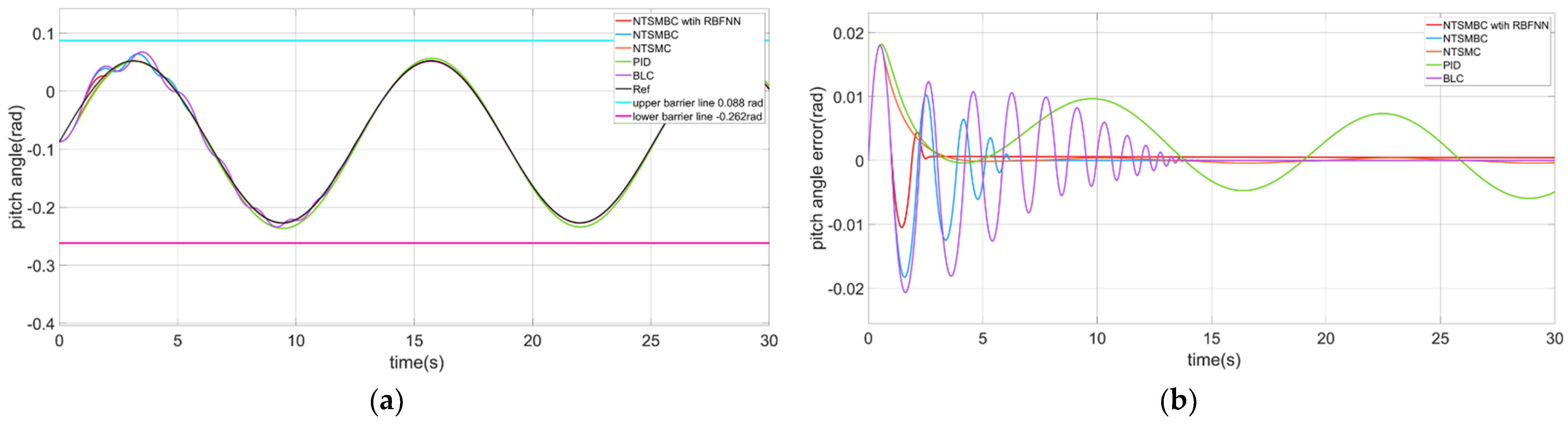
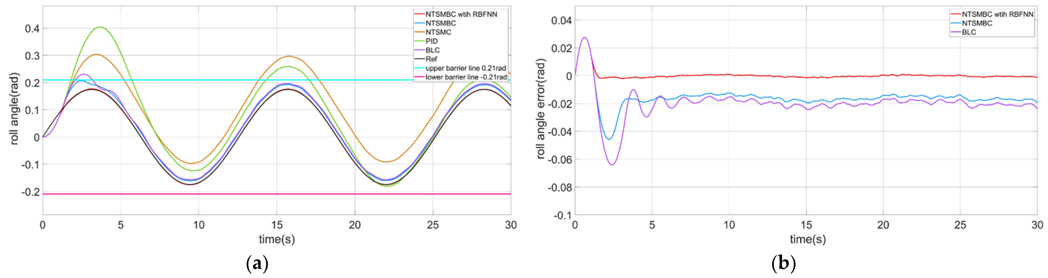
  • When the CDR flies on the water surface, the large attitude angle leads to the water flooding into the cabin or even overturning. Therefore, it is necessary to constrain the attitude angle of the robot. The left and right sides of the robot structure are symmetrical, and a small roll angle can help balance the robot. Thus, the roll angle is constrained symmetrically. The pitch angle is constrained asymmetrically because the front and rear structures of the robot are asymmetric;
  • When the yaw angular velocity reaches the maximum, even if the motor speed continues to increase, the yaw angular velocity cannot be increased. In addition, a large yaw angular velocity causes the robot roll over. Therefore, the yaw angular velocity is controlled by ISMBC algorithm, directly;
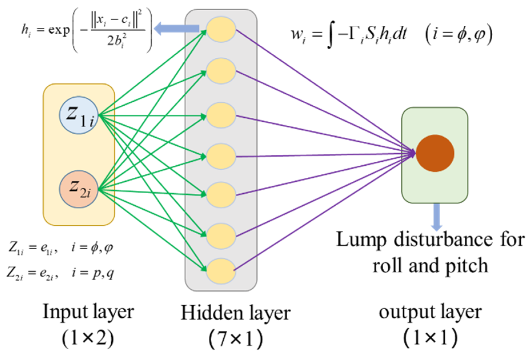
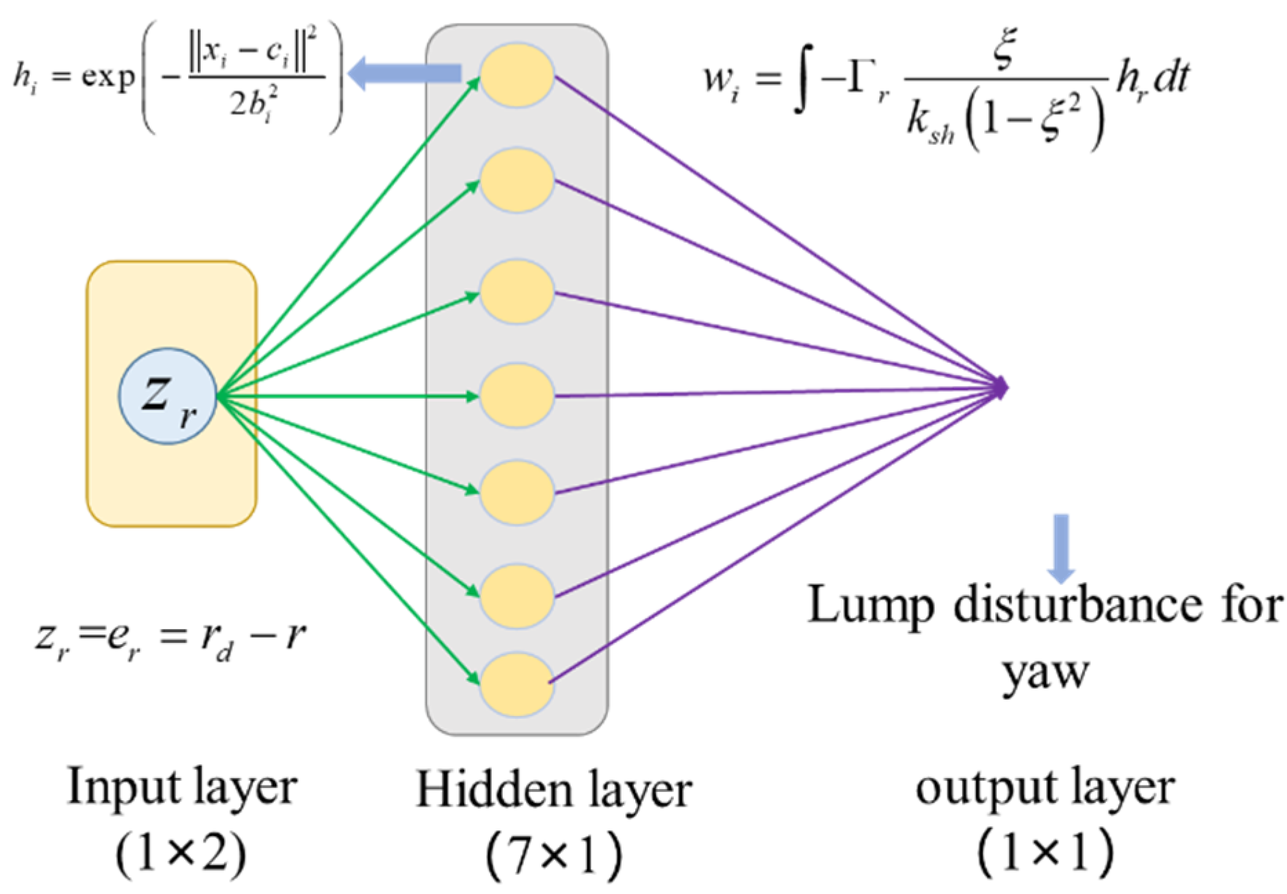
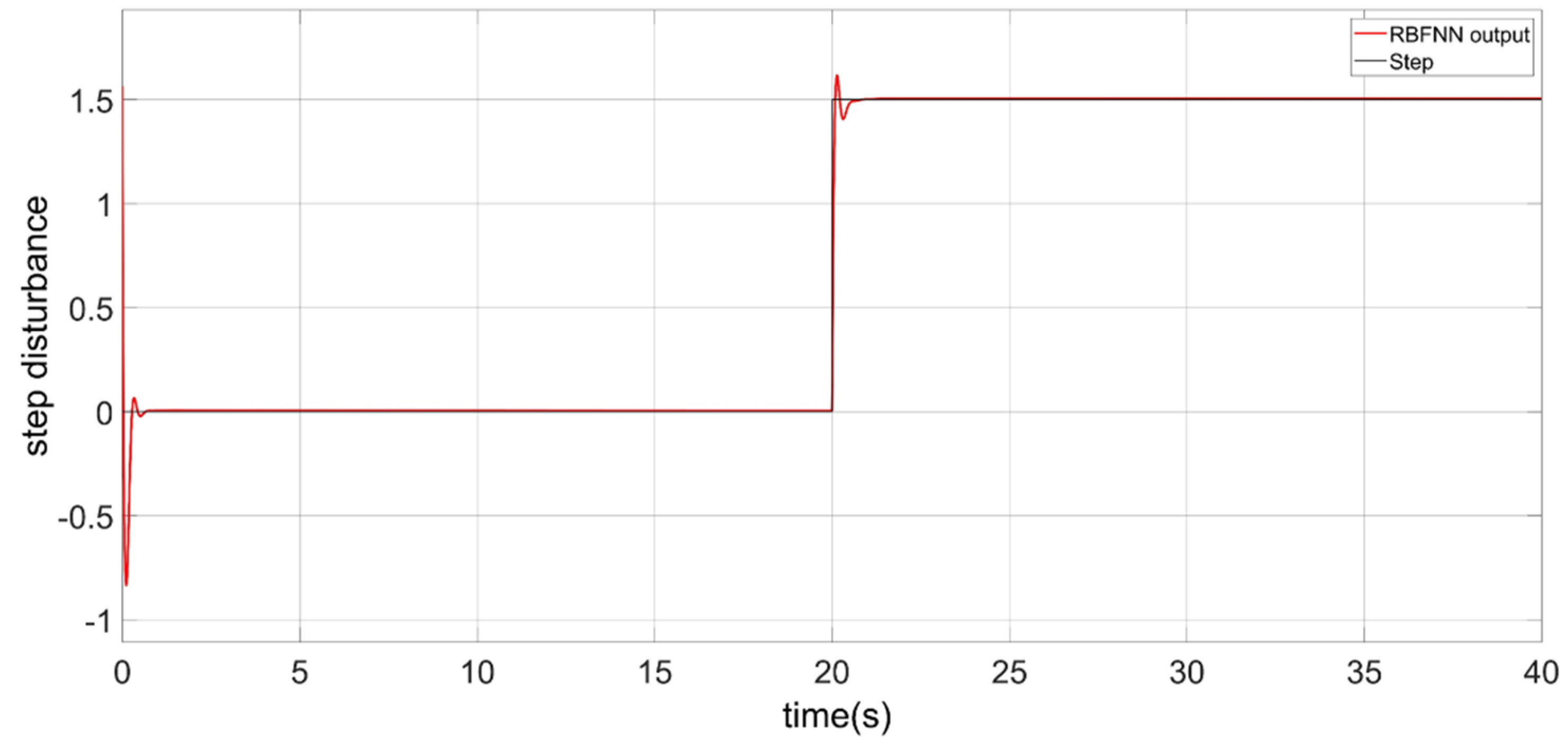
  • There are uncertain parameters and coupling in the dynamic model of the robot attitude. Besides, the attitude of the robot is influenced by the unknown and time-varying water resistance, wind, and current. Thus, the RBFNN is designed for the uncertain lumped disturbances.
Before designing the controllers, we introduced four lemmas to prove the convergence of the controllers in the next part.
Lemma 1 [21,22,23]. The lumped uncertain disturbance can be expressed as: η ( x ) = w T h + ε , w is the neural network weight matrix, h is the output of neurons, h = [ h i ] is the output of the i th neuron in the hidden layer, h i = exp ( x i c i 2 2 b i 2 ) . x is the input vector, c i is the coordinate vector of the center point of the i th neuron Gaussian function in the hidden layer, and b i is the width of the i th neuron Gaussian function. ε is a minimal positive constant. The weight of the RBFNN is:
w = [ ω 1 ω m ] T
The output of the RBFNN is y ( t ) = w T h = ω 1 h 1 + ω 2 h 2 + ω i h i + + ω m h m .
For a continuous function η ( x ) and a minimal positive constant ε , there is an ideal weight vector w * , which makes RBFNN approximate η ( x ) and satisfies max η ( x ) η ^ * ( x ) ε , where w * = arg min θ β ( M θ ) { sup x φ ( M x ) η ( x ) η ^ * ( x ) } . The approximation error can be expressed as ε 0 = η ( x ) η ^ * ( x ) , and ε 0 has an upper bound ε .
Lemma 2 [34]. Let v be any constant such that | v | < 1 . Then, the following inequality is satisfied.
v 2 1 v 2 log ( 1 1 v 2 )
Lemma 3 [34]. Let v be any constant such that | v | < 1 . Then, the following inequality holds:
1 v 1 ( log ( 1 1 v 2 ) ) 1 2
The proof of Lemma 2 and Lemma 3 can be found in the Appendix with the reference [34].
Lemma 4 [28]. Consider the system x = f ( x , u ) . Suppose V ( x ) is a C 1 smooth positive definite function, scalars β 1 , β 2 > 0 , 0 < p < 1 and 0 < δ < 1 such that:
V ( x ) β 1 V ( x ) β 2 V p ( x ) + δ
Then the system x = f ( x , u ) is semi-globally practical finite-time stable (SGPFS).

3. The Design of the CDR Attitude Controllers

According to the problems mentioned in the last section, the robot attitude needs to be constrained when flying on the water surface. The roll angle is constrained within a small angle around 0°, which helps to balance the robot body. The pitch angle needs to be constrained between 5° and −15° according to the fourth, fifth, and sixth lines of Formula (1). The attitude control can be regarded as a second-order single input single output (SISO) nonlinear system. To prevent the loss of generality, we adopted a general mathematical model when designing the controllers.

3.1. Non-Singular Terminal Sliding Mode Asymmetric Barrier Control (NTSMABC)

The second-order nonlinear SISO system with uncertain disturbance is shown in Formula (3):
{ x ˙ 1 = x 2 x ˙ 2 = f ( x ) + g ( x ) u + δ ( x ) y = x 1
where x = [ x 1 x 2 ] T , x 1 and x 2 are the system states, f ( x ) and g ( x ) are smooth functions, δ ( x ) is the external disturbance about the system state, u is the control input, and y is the control output. f ( x ) can be divided into the certain part and the uncertain part. The uncertain part of the system and the extern disturbance can be regarded as the uncertain lumped disturbance. Thus, the system model can be rewritten as:
{ x ˙ 1 = x 2 x ˙ 2 = f 0 ( x ) + g ( x ) u + η ( x ) y = x 1
where f 0 ( x ) is a system certain term and η ( x ) is a lumped uncertain disturbance. Define the positive constants Y _ 0 , Y ¯ 0 . The system state x 1 is satisfied Y _ 0 x 1 Y ¯ 0 . A 0 is the maximum value of the x 1 , and A 0 satisfies max { Y _ 0 , Y ¯ 0 } A 0 k c 1 , k c 1 is the constraint boundary of the system output, | y d | k c 1 . Define k a 1 = k c 1 Y _ 0 , k b 1 = k c 1 Y ¯ 0 , z 1 = y d x 1 and z 1 is satisfied k a 1 < z 1 < k b 1 . If k b 1 = k a 1 = k c 1 A 0 , z 1 is satisfied k b 1 < z 1 < k b 1 , it is the symmetric barrier. The detailed introduction of barrier control can be found in [16].
Define z 2 = α 1 x 2 , where α 1 is a virtual control variable. Then the Lyaunov function V 1 ( z 1 ) is as follows:
V 1 ( z 1 ) = 1 2 q ( z 1 ) log k b 1 2 k b 1 2 z 1 2 + 1 2 ( 1 q ( z 1 ) ) log k a 1 2 k a 1 2 z 1 2
where q ( z 1 ) = { 0 , 0 < z 1 < k b 1 1 , k a 1 < z 1 0 .
V 1 ( z 1 ) takes the derivative of time t, which yields:
V ˙ 1 ( z 1 ) = q ( z 1 ) k b 1 2 k b 1 2 z 1 2 z 1 z ˙ 1 + ( 1 q ( z 1 ) ) k a 1 2 k a 1 2 z 1 2 z 1 z ˙ 1
Since x 2 = α 1 z 2 , z ˙ 1 = y ˙ d x 2 = y ˙ d α 1 + z 2 , the virtual state is defined as α 1 = k 1 z 1 + y ˙ d . where k 1 is a positive constant. Substituting z ˙ 1 and α 1 into Formula (6) obtains:
V ˙ 1 ( z 1 ) = k 1 k b 1 2 ( q ( z 1 ) k b 1 2 z 1 2 + ( 1 q ( z 1 ) ) k a 1 2 z 1 2 ) z 1 2 + k b 1 2 ( q ( z 1 ) k b 1 2 z 1 2 + 1 q ( z 1 ) k a 1 2 z 1 2 ) z 1 z 2
The non-singular terminal sliding surface is S = z 2 + 1 β z 1 p q , S ˙ = z ˙ 2 + p β q z 1 p q 1 z ˙ 1 . The sliding mode approach law is designed as S ˙ = k 2 S + k 3 | S | 1 2 s i g n ( s ) .
The Lyapunov function V 2 is defined as:
V 2 = V 1 + 1 2 S 2
The Formula (8) takes the derivative of time t and substitutes it into Formula (7) and S ˙ obtains:
V ˙ 2 = V ˙ 1 + S S ˙ = k 1 k b 1 2 Q ( z 1 ) z 1 2 + k b 1 2 Q ( z 1 ) z 1 z 2 + S ( z ˙ 2 + p β q z 1 p q 1 z ˙ 1 ) = k 1 k b 1 2 Q ( z 1 ) z 1 2 + k b 1 2 Q ( z 1 ) z 1 z 2 + S ( α ˙ 1 x ˙ 2 + p β q z 1 p q 1 z ˙ 1 ) = k 1 k b 1 2 Q ( z 1 ) z 1 2 + k b 1 2 Q ( z 1 ) z 1 z 2 + S ( α ˙ 1 f 0 ( x ) g ( x ) u η ( x ) + p β q z 1 p q 1 z ˙ 1 )
where Q ( z 1 ) = q ( z 1 ) k b 1 2 z 1 2 + ( 1 q ( z 1 ) ) k a 1 2 z 1 2 .
Define α ˙ 1 f 0 ( x ) g ( x ) u η ( x ) + p β q z 1 p q 1 z ˙ 1 = k 2 S + k 3 | S | 1 2 s i g n ( s ) .
When the lumped disturbance is known, the controller can be designed as:
u = 1 g ( x ) [ f 0 ( x ) η ( x ) + α ˙ 1 + p β q z 1 p q 1 z ˙ 1 + k b 1 2 Q ( z 1 ) z 1 + k 2 S + k 3 | S | 1 2 s i g n ( s ) ]
where β , k 2 , k 3 are positive constants, p / q = 2 * n 1 , n = 1 , 2 , 3 and p q . In the controller (10), the functions g ( x ) and f 0 ( x ) are known. However, the lumped disturbance caused by external disturbances and uncertain parameters is unknown; therefore, the controller designed by Formula (10) cannot control the system.
Therefore, the RBFNN is designed to approximate the lumped disturbance in Formula (4). The definition is η ( x ) = ε 0 + η ^ * ( x ) = ε 0 + w * T h , w ˜ = w ^ w * , w * is the optimal weight, w ^ is an estimate of w * , and w * is constant, so w ˜ ˙ = w ^ ˙ .
Define the Lyapunov function V 3 :
V 3 = V 1 + 1 2 S 2 + 1 2 t r ( w ˜ T Γ 1 w ˜ )
Γ is a positive definite matrix, Formula (12) can be obtained by V 3 taking the derivative of time t.
V 3 = V ˙ 1 + S S ˙ + w ˜ T Γ 1 w ^ ˙
Substituting η ( x ) = ε 0 + w * T h into Formula (12):
V ˙ 3 = V ˙ 1 + S S ˙ + w ˜ T Γ 1 w ^ ˙ = k 1 k b 1 2 Q ( z 1 ) z 1 2 + k b 1 2 Q ( z 1 ) z 1 z 2 + S ( α ˙ 1 f 0 ( x ) g ( x ) u w T * h ε 0 + p β q z 1 p q 1 z ˙ 1 ) + w ˜ T Γ 1 w ^ ˙
The controller is designed as:
u = 1 g ( x ) [ f 0 ( x ) w ^ T h + α ˙ 1 + p β q z 1 p q 1 z ˙ 1 + k b 1 2 Q ( z 1 ) z 1 + k 2 S + k 3 | S | 1 2 s i g n ( s ) ]
Substituting Formula (14) into Formula (13) can obtain:
V ˙ 3 = k 1 z 1 2 1 β ( q ( z 1 ) k b 1 2 z 1 2 + 1 q ( z 1 ) k a 1 2 z 1 2 ) z 1 P / q + 1 + w ˜ T ( S h + Γ 1 w ^ ˙ ) k 2 S 2 S ( ε 0 + k 3 | S | 1 2 s i g n ( s ) )
The adaptive law of the RBFNN weight is designed as:
w ^ ˙ = Γ S h
Substituting Formula (16) into Formula (15) can obtain:
V ˙ 3 = k 1 k b 1 2 Q ( z 1 ) z 1 2 1 β k b 1 2 Q ( z 1 ) z 1 P / q + 1 k 2 S 2 S ( ε 0 + k 3 | S | 1 2 s i g n ( S ) )
When q ( z 1 ) = 1
V ˙ 3 = k 1 k b 1 2 k b 1 2 z 1 2 z 1 2 1 β k b 1 2 k b 1 2 z 1 2 z 1 P / q + 1 k 2 S 2 S ε 0 k 3 | S | 1 2 S s i g n ( S )
Because p / q + 1 = 2 n , n = 1 , 2 , 3 , z 1 2 < k b 1 2 , | ε 0 | ε , ε is a minimal normal constant.
When S > 0 , ε 0 > 0 , V ˙ 3 0 . When ε 0 > 0 , S < 0 , a parameter always exists, k 3 , which satisfies k 3 | S | 3 2 > | S | ε , so V ˙ 3 < 0 . When S > 0 , ε 0 < 0 , parameter k 3 always exists, which satisfies k 3 | S | 3 2 > | S | ε , so V ˙ 3 < 0 . When S < 0 , ε 0 < 0 , V ˙ 3 0 .
When q ( z 1 ) = 0
V ˙ 3 = k 1 k b 1 2 k a 1 2 z 1 2 z 1 2 1 β k b 1 2 k a 1 2 z 1 2 z 1 P / q + 1 k 2 S 2 S ε 0 k 3 | S | 1 2 S s i g n ( S )
Because z 1 2 < k a 1 2 , when S > 0 , ε 0 > 0 , V ˙ 3 0 . When S < 0 , ε 0 > 0 , parameter k 3 always exists, which stratifies k 3 | S | 3 2 > | S | ε , V ˙ 3 < 0 . When S > 0 , ε 0 < 0 , parameter k 3 always exists, which satisfies k 3 | S | 3 2 > | S | ε . When S > 0 , ε 0 > 0 , V ˙ 3 0 .
V 3 is a continuous and derivable function. V 3 0 and only at point zero V 3 = 0 . Because V ˙ 3 0 , z 1 , z ˙ 1 , S , S ˙ are uniformly bounded, thus, V ¨ 3 is bounded. According to Barbalat’s lemma, when t , V 3 0 , V ˙ 3 0 , so that the state errors converge.
The proposed algorithm combines barrier control with NTSMC. Compared with the NTSMC, the proposed algorithm adds the term that can constrain the system state. The algorithm inherits the robustness of NTSMC. The convergence speed of the state errors is improved, because the exponential term is introduced into the sliding mode surface.

3.2. Adaptive Integral Sliding Mode Barrier Control

The yaw angle does not need to be constrained, but the yaw angular velocity needs to be constrained. To make the controller more robust, we combined ISMC with BC and designed an adaptive law for the sliding mode surface.
The second-order nonlinear SISO control system with uncertain disturbance is shown in Formula (4):
{ x ˙ 1 = x 2 x ˙ 2 = f 0 ( x ) + g ( x ) u + η ( x ) y 1 = x 1
where η ( x ) is the uncertain lumped disturbance. The RBFNN is used to approximate η ( x ) , η ( x ) = ε 0 + w * T h . Definition w ˜ = w ^ w * , w * is the optimal weight, w ^ is the estimation of w * , w * is a constant, w ˜ ˙ = w ^ ˙ . ε 0 is the approximation residual of the RBFNN. Thus, the second line of Formula (4) can be rewritten as:
x ˙ 2 = f 0 ( x ) + g ( x ) u + w T * h + ε 0
where, x 1 , x 2 , y d , y ˙ d are derivable and continuous. When designing the controller, the system is divided into two parts, which are the outer loop and the inner loop. For the outer loop control, define z 1 = y d x 1 , S 1 = z 1 + λ 1 z 1 d t , S ˙ 1 = ( y ˙ d x 2 d ) + λ 1 z 1 , where λ 1 is a positive constant.:
x 2 d = k 4 S 1 + λ 1 z 1 + y ˙ d + k 5 s i g n ( S 1 )
where x 2 d is the control input of the outer loop, where k 4 , k 5 are positive constants. Define the Lyapunov function V 4 = 1 2 S 1 2 , V 4 takes the derivative of time t and substitutes it to x 2 d which yields:
V ˙ 4 = S 1 S ˙ 1 = S 1 ( y ˙ d x 2 d + λ 1 z 1 ) = k 4 S 1 2 k 5 | S 1 | 0
Therefore, t , z 1 0 . For the inner loop control, define z 2 = x 2 d x 2 , the integral sliding surface S 2 = z 2 + λ 2 z 2 p / q d τ , where λ 2 is a positive constant, p / q = 2 * n 1 , n = 1 , 2 , 3 . Because z 2 is bounded, if the system state error converges in finite time, z 2 p / q d τ is bounded, so | S 2 | k s h , k s h is a positive constant which is the upper limit of the sliding surface. Define the control law u = 1 g ( x ) ( u 1 + u 2 ) . The control law consists of two parts which will be designed below.
Define the virtual variable ξ = S 2 / k s h , ξ ˙ = S ˙ 2 / k s h . The Lyapunov function V 5 is
V 5 = 1 2 log ( 1 1 ξ 2 ) + 1 2 t r ( w ˜ T Γ 1 w ˜ )
where Γ is a positive definite matrix. Formula (21) takes the derivative of time t as:
V ˙ 5 = ξ ξ ˙ 1 ξ 2 + 1 2 w ˜ T Γ 1 w ˜ ˙
Substituting Formula (18) into Formula (22) can obtain:
V ˙ 5 = ξ k s h ( 1 ξ 2 ) ( y ¨ d f 0 ( x ) g ( x ) u w * T h ε 0 + λ 2 z 2 p / q ) + 1 2 w ˜ T Γ 1 w ˜ ˙
The definition of the control law is:
u 1 = 1 g ( x ) ( f 0 ( x ) + y ¨ d + k 6 S + λ 2 z 2 p / q + w ^ T h ) ,   u 2 = k 7 g ( x ) s i g n ( S )
where k 6 is a positive constant and k 7 changes with the system state error to prevent the system state exceeds the constraint boundary. Substituting u 1 , u 2 into Formula (23) can obtain:
V ˙ 5 = ξ k s h ( 1 ξ 2 ) ( k 6 S + w ˜ T h ε 0 k 7 s i g n ( S ) ) + w ˜ T Γ 1 w ^ ˙ = k 6 ξ 2 1 ξ 2 ξ s i g n ( S ) k s h ( 1 ξ 2 ) k 7 + w ˜ T ( Γ 1 w ^ ˙ + ξ k s h ( 1 ξ 2 ) h ) ξ ε 0 k s h ( 1 ξ 2 )
The adaptive law of the RBFNN weight is designed as follows:
w ^ ˙ = Γ ξ k s h ( 1 ξ 2 ) h
Substituting Formula (26) into Formula (25) can obtain:
V ˙ 5 = k 6 ξ 2 1 ξ 2 ξ s i g n ( S ) k s h ( 1 ξ 2 ) k 7 ε ξ
where ε ξ = ξ ε 0 k s h ( 1 ξ 2 ) , when z 2 0 , ε ξ 0 .
s i g n ( S ) = S | S | S | k s h | | ξ | , s i g n ( S ) S | k s h | | ξ | , rewrite Formula (27) to obtain:
V ˙ 5 k 6 ξ 2 1 ξ 2 ξ k s h ( 1 ξ 2 ) S | k s h | | ξ | k 7 ε ξ = k 6 ξ 2 1 ξ 2 ξ k s h ( 1 ξ 2 ) ξ k s h | k s h | | ξ | k 7 ε ξ = k 6 ξ 2 1 ξ 2 k 7 ξ 2 k s h ( 1 ξ 2 ) | ξ | ε ξ
Because k 7 ξ 2 k s h ( 1 ξ 2 ) | ξ | ξ 2 k s h ( 1 ξ 2 ) k 7 ( 1 | ξ | ) | ξ | = | ξ | k s h ( 1 ξ 2 ) k 7 ( 1 | ξ | ) .
Rewrite Formula (28) to obtain:
V ˙ 5 k 6 ξ 2 1 ξ 2 | ξ | k s h ( 1 ξ 2 ) ( 1 | ξ | ) k 7 + | ε ξ |
Definition k 7 = 1 1 | ξ | ( | S | | ξ | k 8 ) , where k 8 is a positive constant. Substitute it into (29) which gives:
V ˙ 5 k 4 ξ 2 1 ξ 2 k 5 ξ 2 1 ξ 2 1 | ξ | + | ε ξ |
According to the Lemmas 2 and 3, Formula (30) satisfies:
V ˙ 5 k 1 V 5 k 3 V 5 V 5 1 2 + | ε ξ | = k 1 V 5 k 3 V 5 1 2 + | ε ξ |
According to the Lemma 4, the system is SGPFS, so the system state errors can converge in the finite time.
Compared with the traditional ISMC, the AISMBC can adaptively adjust the gain of the sliding mode based on the error of the actual state and boundary. Therefore, the system state is constrained, and the influence of the lump disturbance on the system can be suppressed by increasing the gain of the sliding mode. Thus, the robustness of the controller is improved.

4. Simulation Results and Discussion

4.1. Design for the Controllers for CDR Flying on the Water Surface

To ensure the safety of the robot flying on the water surface, the roll angle and pitch angle need to satisfy φ [ 12 12 ] and θ [ 15 5 ] . The yaw angular velocity of the robot needs to satisfy r [ 0 . 3   rad / s 0 . 3   rad / s ] .
According to Formula (14), the pitch angle controller and roll angle controller are designed as:
{ u ϕ = I x l [ w ^ T ϕ h ϕ + α ˙ ϕ + p β q z ϕ p q 1 z ˙ ϕ + k b ϕ 2 q ( z ϕ ) k b ϕ 2 z ϕ 2 z ϕ + k 2 ϕ S ϕ + k 3 ϕ | S ϕ | 1 2 s i g n ( S ϕ ) ] u θ = I y l [ w ^ T θ h θ + α ˙ θ + p β q z θ p q 1 z ˙ θ + ( k b θ 2 q ( z θ ) k b θ 2 z θ 2 + k a θ 2 ( 1 q ( z θ ) ) k a θ 2 z θ 2 ) z θ + k 2 θ S θ + k 3 θ | S θ | 1 2 s i g n ( S θ ) ]
NTSMBC is used to control the roll angle and the pitch angle. S i = z 2 i + 1 β z 1 i p q , ( i = ϕ , θ ) , z 1 i is the angle error between the desired angle and the actual angle. The structure of the RBFNN for the roll angle and pitch angle is shown in Figure 4:
The input layer of the neural network includes two inputs: the angle error and angular velocity error. The output of the neural network is the uncertain lumped disturbance. The hidden layer consists of seven neurons. The central vector matrix of the Gaussian function of neurons is
C = [ 0.4 0.2 0.1 0 0.1 0.2 0.4 0.4 0.2 0.1 0 0.1 0.2 0.4 ] , the base width of the Gaussian function is designed as b = 0.1 . According to Formula (16), the adaptive law of the RBFNN weight is designed as:
w ^ ˙ i = Γ i S i h i ( i = ϕ , φ )
AISMBC is adopted in the yaw angular velocity control. Based on Formula (22), the controller is designed as follows:
u r = 1 I z ( ψ ¨ d + k 4 S r + λ z r p / q + w r T h r + k 5 s i g n ( S r ) )
where S r = z r + λ z r p / q d τ , z r is the yaw angular velocity error. The controller parameters were discussed in the Section 3. The structure of the yaw angular velocity neural network is shown in Figure 5.
The input layer of the RBFNN only has the yaw angular velocity error, and the output of the neural network is the lump disturbance. The hidden layer includes seven neurons. The center vector matrix of the Gaussian function of neurons is C = [ 0.4 0.2 0.1 0 0.1 0.2 0.4 ] and the base width of the Gaussian function is b = 0.2 .
According to Formula (24), the weight update law of the RBFNN can be designed as:
w ^ ˙ r = Γ r ξ k s h ( 1 ξ 2 ) h r

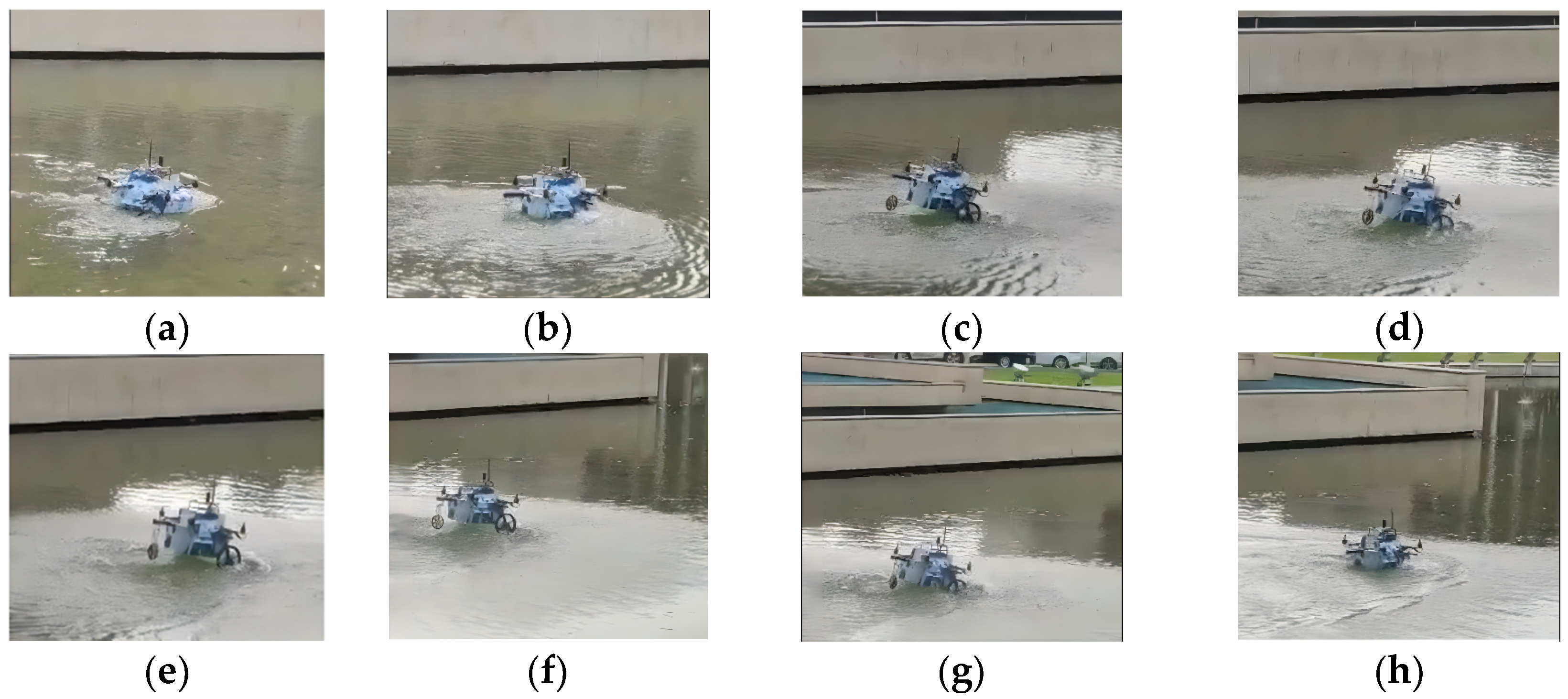
4.2. Simulation Results of the CDR Flying on Water Surface

To verify the effectiveness of our proposed algorithm, the NTSMABC was adapted to the pitch angle control and the roll angle control. The control results were compared with PID control, BLC, and NTSMC, respectively. For the yaw angular velocity control, AISMBC was adapted. The control results were compared with ISMC and PID control. At last, NTSMABC and AISMBC were used to control the CDR to track the desired circular trajectory. The control block diagram of the robot flying on the water surface is shown in Figure 6.

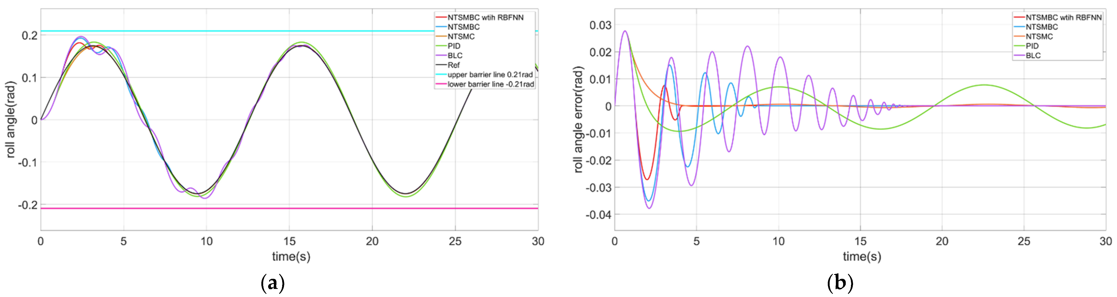
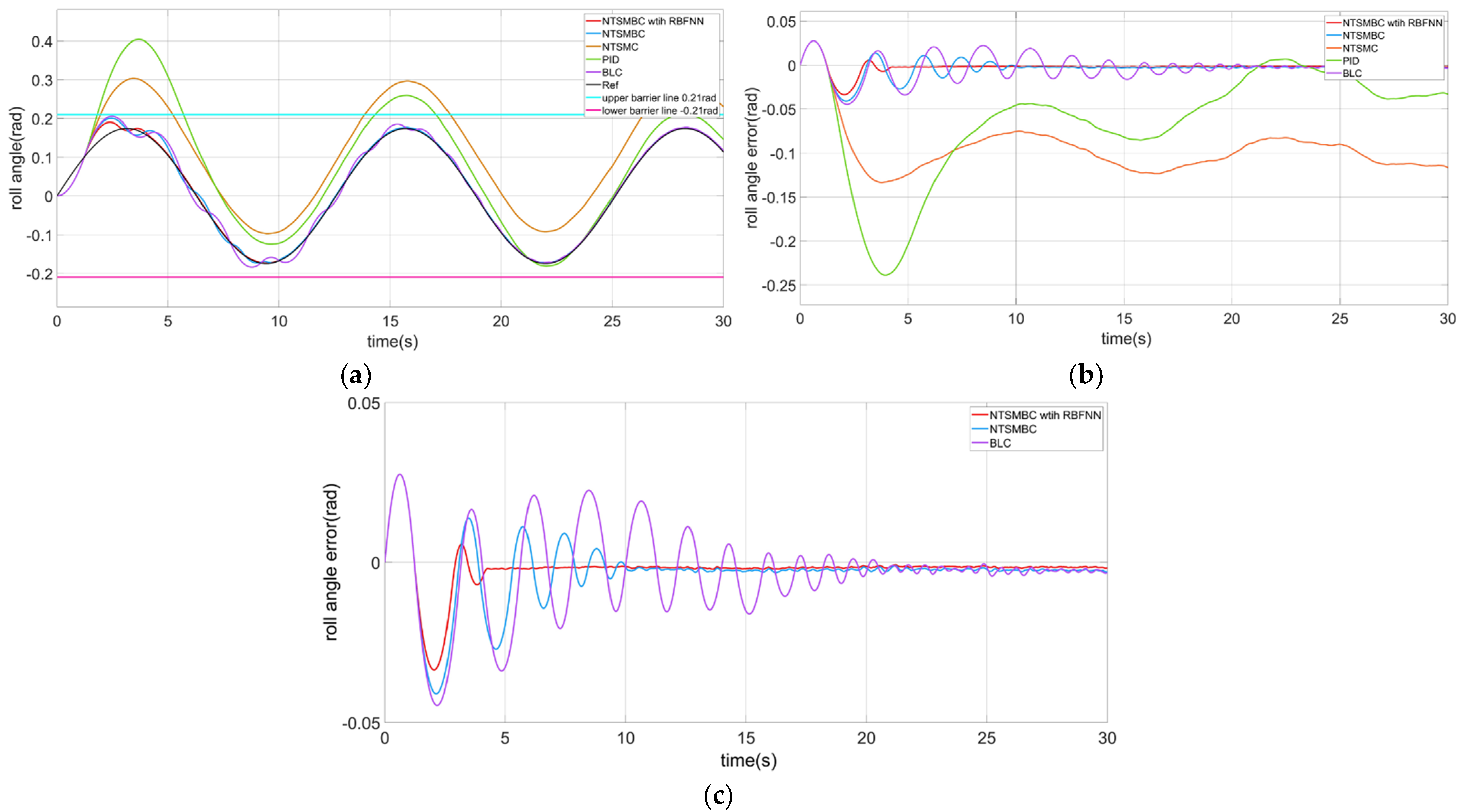
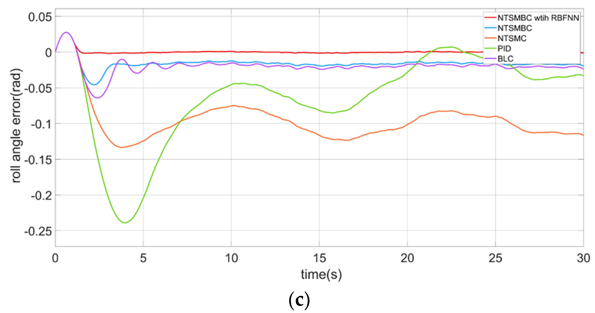
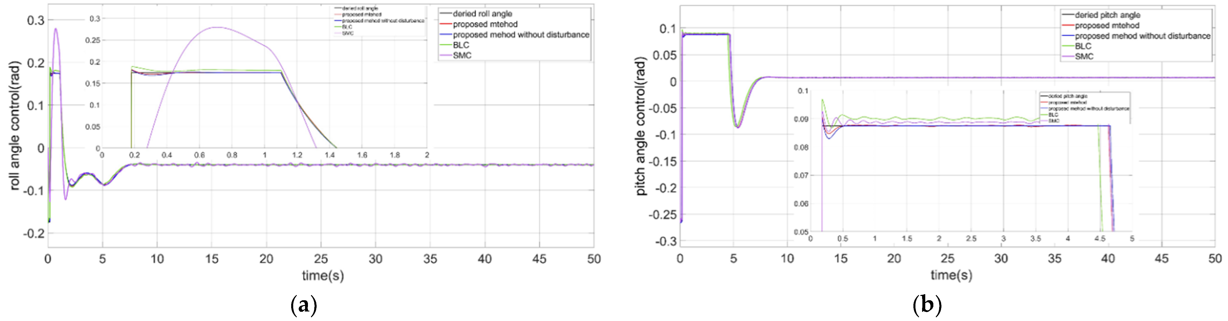
4.2.1. The Roll Angle Control of the CDR

The parameters of the roll angle controllers are shown in Table 1.
The desired roll angle was designed as φ d = 0.1745 * sin ( 0.5 t ) , when there are no uncertain model parameters and external disturbances in the dynamic model of the roll angle. The control results of the roll angle are shown in Figure 7.
As shown in Figure 7a, the robot could track the desired roll angle when the four control methods were adopted, and the roll angle did not exceed the safety boundary of 0.2094 rad (12°). As shown in Figure 7b, BLC had some oscillation and needed to be over 15 s to be in a stable state (the purple line). For the NTSMBC without RBFNN, the maximum tracking error was about 0.03 rad, and the error convergence time was about 8 s, which was longer than NTSMBC with RBFNN. When there was no uncertain disturbance, the control results of NTSMC (orange line) were the best without oscillation and tracking errors, but the proposed method had the fastest convergence speed.
To simulate the influence of water resistance, wind disturbance, and current on the robot flying on the water surface, the random disturbance with a mean value of 1 and variance of 0.1 was applied to the robot roll angular acceleration. The control results are shown in Figure 8.
As shown in Figure 8, the PID controller oscillated in a large range and could not track the desired angle. NTSMC (orange line) had a static error of about 0.1 rad, but the maximum tracking error was less than PID, which was because NTSMC had a strong robustness. These two control methods exceeded the safety boundary 0.2094 rad (12°). The BLC (purple line) ensured that the roll angle was less than the safety boundary, but it oscillated for a long time. The proposed NTSMBC ensured the roll angle was smaller than the safety boundary, and the oscillation was smaller and the convergence speed was faster than BLC. As shown in Figure 8c, when the control output of NTSMBC was compensated by RBFNN (red line), the maximum tracking error was 0.02 rad, and the error converged at 2.5 s. NTSMBC inherited the robustness of NTSMC. When there was an uncertain lumped disturbance, it could follow the desired roll angle even without the compensation of RBFNN.
The roll angle RBFNN outputs are shown in Figure 9.

4.2.2. The Pitch Angle Control of the CDR

The parameters of the pitch angle controller are shown in Table 2.
The NTSMABC was used to control the pitch angle. The upper boundary of the pitch angle was 0.0873 rad (5°) and the lower boundary was −0.2618 rad (−15°). The desired pitch angle was designed as θ d = 0 . 1396 * sin ( 0.5 t ) 0.0873 . The initial pitch angle was set to −5°.
When there were no uncertain model parameters and external disturbances in the dynamic model of the pitch angle, the results of the pitch control are shown in Figure 10.
As shown in Figure 10a, the results of the four control methods did not exceed the safety boundary of 0.0873 rad (5°) and −0.2618 rad (−15°). As shown in Figure 10b, the convergence time of the BLC was longer than other methods (pink line). PID control (green line) had a tracking error about 0.01 rad. The convergence speed of NTSMBC was faster than the BLC and the convergence time of error was about 7 s. When RBFNN compensated for the NTSMBC output, the convergence speed of NTSMBC was faster than NTSMBC, which required about 3 s. The results of the pitch control were similar to the roll angle control results.
The robot pitch angular acceleration was subjected to a random disturbance with a mean value of −1 and a variance of 0.1, which was to simulate the uncertain water resistance, wind disturbance, and current. The control results are shown in Figure 11.
As shown in Figure 11a, the PID controller had a large oscillation, and the maximum tracking error was about 0.18 rad. NTSMC had about a 0.1 rad static error. The pitch angle exceeded the lower limit of the safety boundary −0.2618 rad (−15°) when the robot adopted the PID control and NTSMC. BLC (purple line) could control the pitch angle in the safe range. However, it oscillated for a long time. NTSMBC ensured that the pitch angle was smaller than the safety boundary. The oscillation was smaller than PID and NTSMC and the convergence speed was faster than PID and NTSMC. As shown in Figure 11c, when the control output of NTSMBC was compensated by RBFNN (red line), the maximum tracking error was 0.02 rad, and the time of error convergence was about 2.5 s.
The output of the pitch angle RBFNN is shown in Figure 12:
When using the NTSMBC algorithm and the BLC algorithm to control the pitch angle and roll angle, the control results oscillated. The reason was the boundary was too strict. In fact, it is not necessary to set the constraint boundary completely according to the actual limitation. The suitable boundary parameters ka and kb can be selected to achieve the purpose of constraint robot attitude. When controlling the roll angle, set the relaxation boundary kb = 0.15. Moreover, the random lumped disturbance with a mean value of −1 and variance of 0.1 was applied to the robot roll angular acceleration. The control results are shown in Figure 13.
With the relaxed boundary, the roll angle control oscillation decreased. However, the static error of BLC (purple line) and NTSMBC (blue line) was about 0.02 rad, as shown in Figure 13c. This was because the boundary was too loose, while BLC exceeded the set safety boundary, and NTSMBC was close to the set safety boundary. NTSMBC with RBFNN compensation (red line) could follow the desired angle and had a fast convergence speed and no static error or oscillation. Compared with the roll angle control with strict constraints, choosing the appropriate constraint boundary can not only constrain the angle state, but can also improve the performance of the controller.

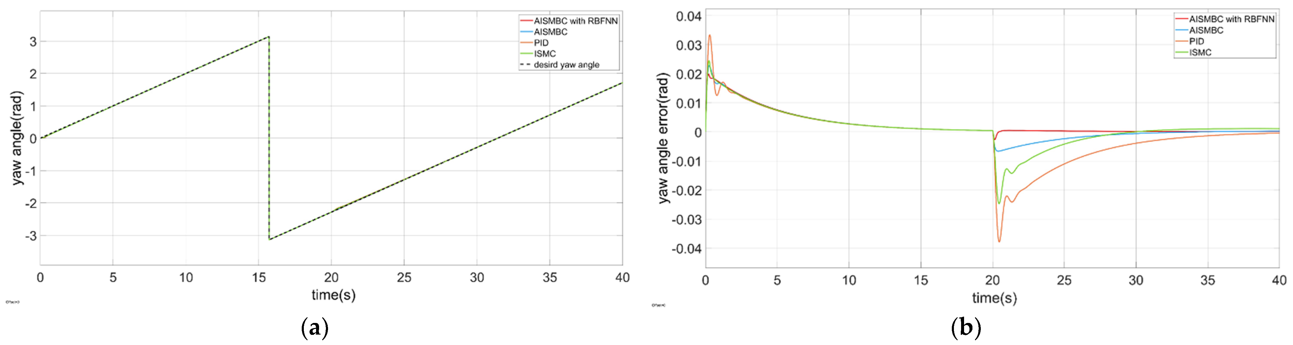
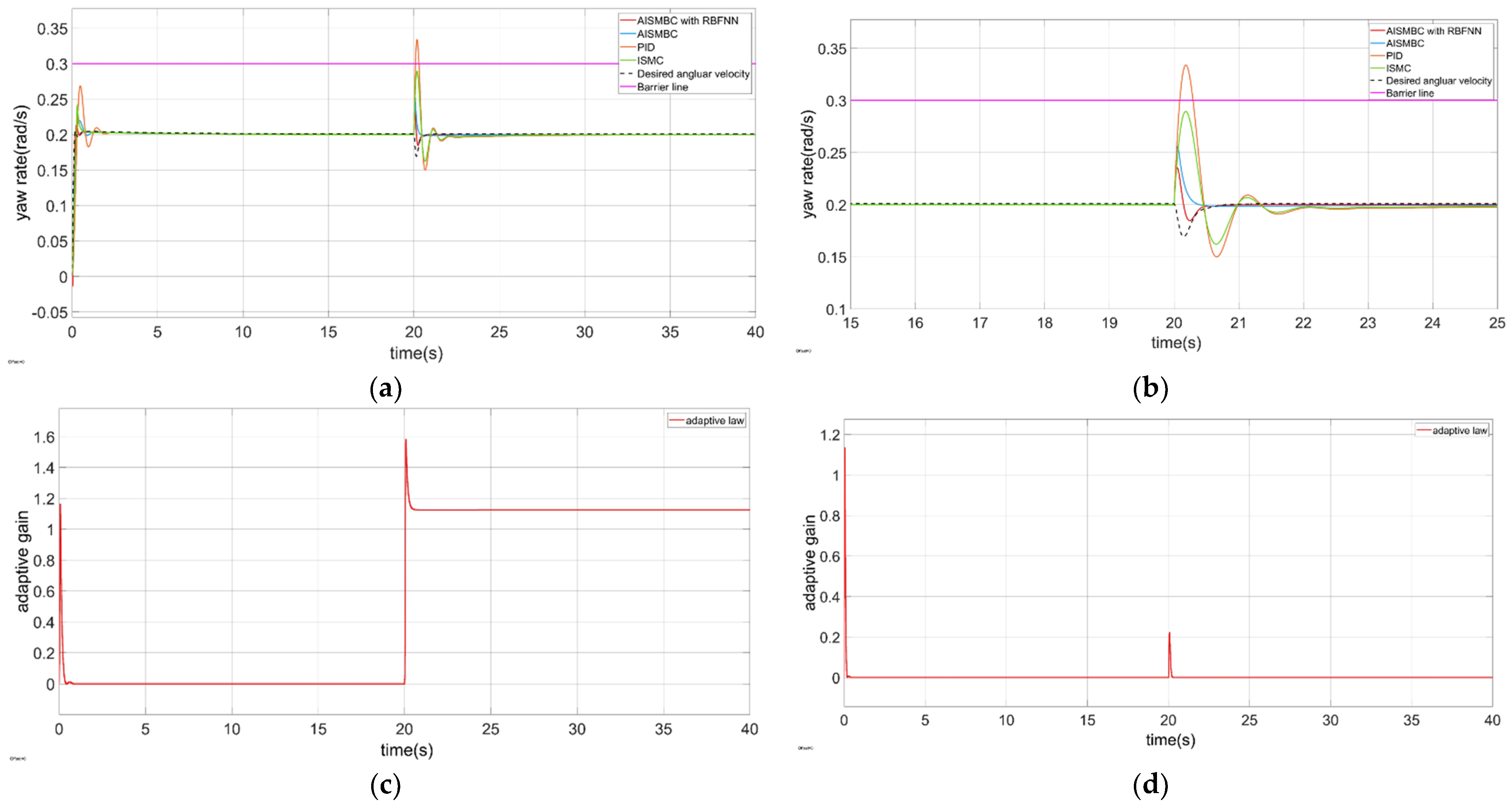
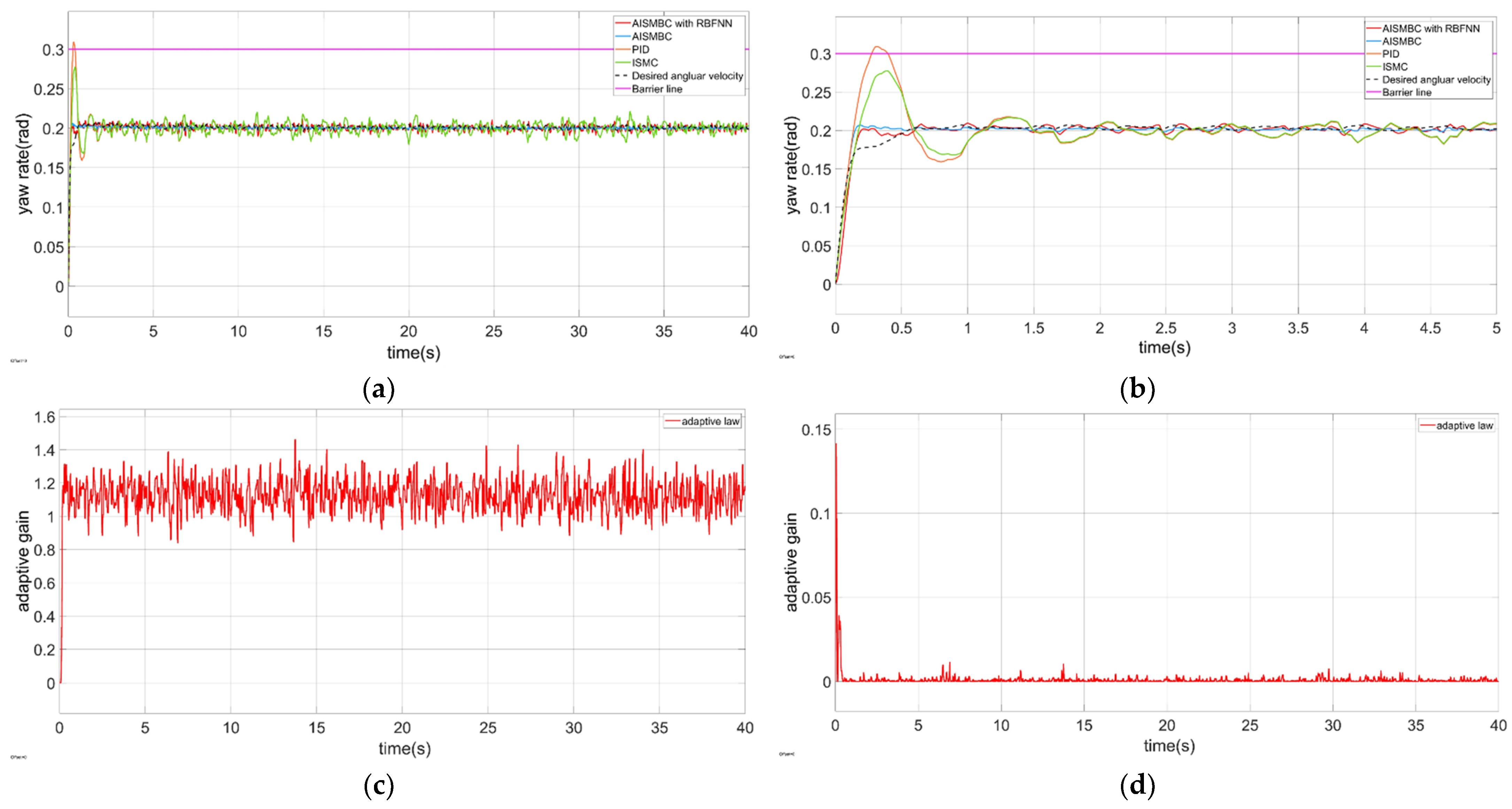
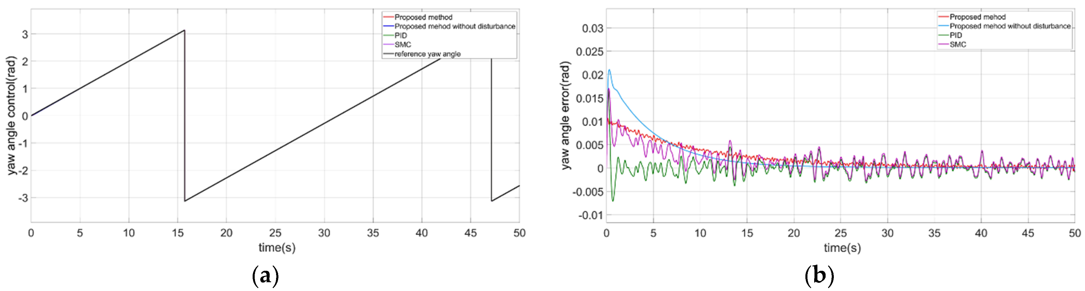
4.2.3. The Yaw Angle Control of the CDR

The parameters of the yaw angle controller are shown in Table 3.
The desired yaw angular velocity was ω d = 0.2 rad/s. There was no uncertain lumped disturbance before 20 s. At 20 s, a step disturbance of 1.5 was applied to the yaw angular acceleration. The yaw angle control results are shown in Figure 14.
As shown in Figure 14, the desired yaw angular velocity was 0.2 rad/s; therefore, the desired yaw angle changed from 0 to π. At 20 s, a step disturbance was applied to the acceleration of the yaw angle. The tracking error of AISMBC (blue line) was less than 0.01 rad. ISMC was about 0.025 rad, and PID control was about 0.04 rad. The AISMBC with RBFNN was almost unaffected by the step disturbance, as shown by the red line.
The yaw angular velocity control is shown in Figure 15.
As shown in Figure 15a, the robot could follow the desired yaw angular velocity with the three methods, but there was an overshoot in the PID control and ISMC. At 20 s, the step disturbance was applied to the yaw angle acceleration, and the PID controller (orange line) exceeded the safety boundary. The maximum tracking error of ISMBC (green line) was about 0.08 rad/s. The maximum tracking error of AISMBC (blue line) was about 0.05 rad/s. The maximum tracking error of AISMBC with RBFNN compensation (red line) was 0.03 rad/s. The adaptive gain of AISMBC is shown in Figure 15c. When the angular velocity tracking error was small, the gain of the sliding mode was almost zero. When the disturbance was applied, the gain of sliding mode increased. Therefore, the robustness of AISMBC improved. The adaptive gain of AISMBC with the RBFNN compensation is shown in Figure 15d. The controller output was compensated by the RBFNN. Thus, a large sliding mode gain was not needed. The output of the RBFNN is shown in Figure 16.
To further verify the robustness of the controller, the random disturbance with a mean value of 1.5 and a variance of 0.1 was applied to the yaw angular acceleration to simulate the uncertain lump disturbance. The yaw angular velocity control is shown in Figure 17.
As shown in Figure 17a,b, the PID controller (orange line) exceeded the boundary 0.3 rad/s, and the ISMC (green line) had an overshoot of about 0.08 rad/s, which was close to the safety boundary. Compared with AISMBC, the PID control and ISMC had a weaker ability to suppress the noise. The adaptive gain of AISMBC is shown in Figure 17c. The adaptive gain of AISMBC with RBFNN is shown in Figure 17d.
The output of yaw angular velocity RBFNN is shown in Figure 18.

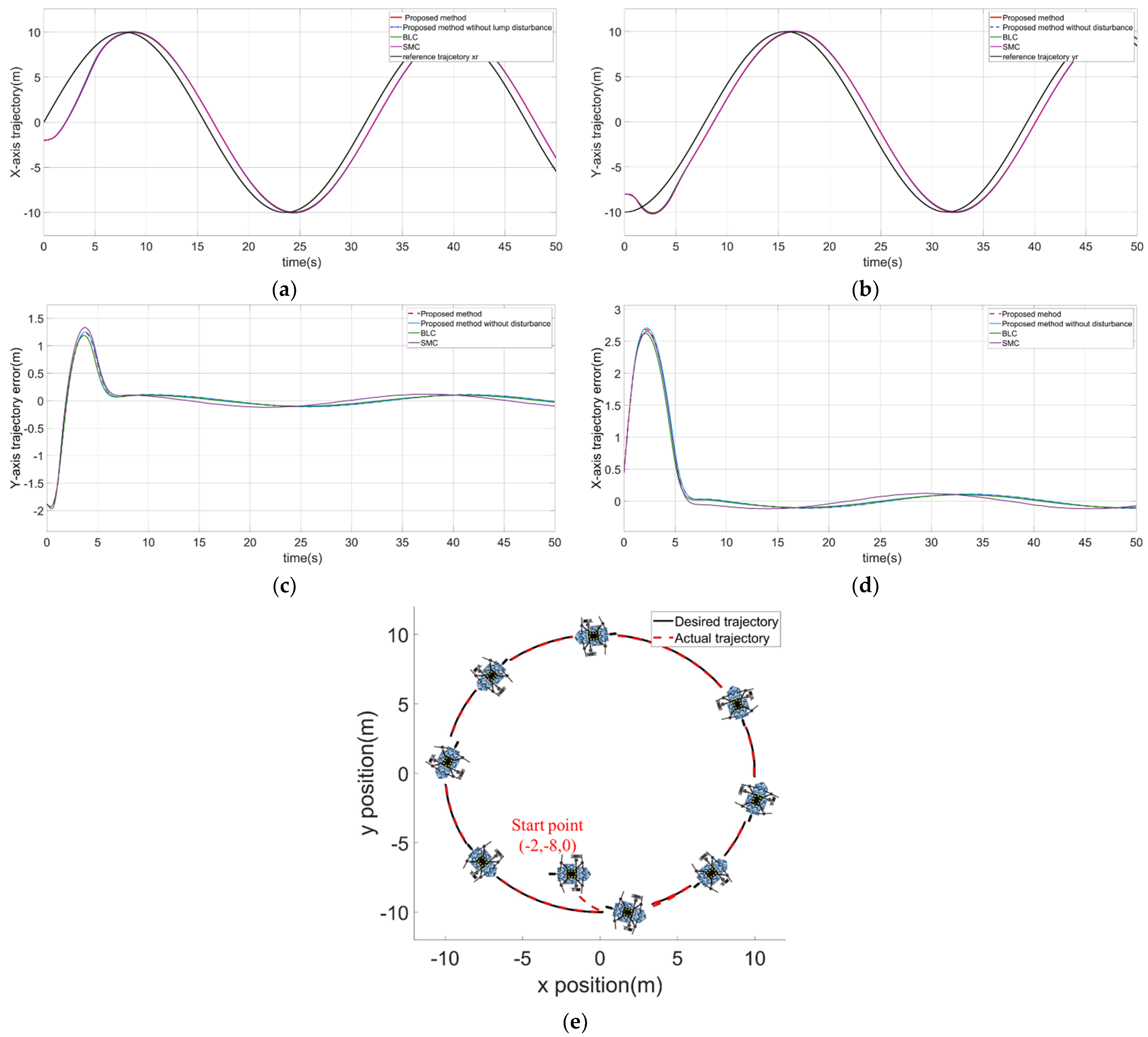
4.2.4. The CDR Tracks the Circular Desired Trajectory on the Water Surface

The desired trajectory was designed as a circular trajectory with the radius R = 10   m and a yaw angular velocity ω = 0.2 rad/s. The desired position is defined by Formula (36):
{ x r = R * sin ( ω * t ) y r   = R * cos ( ω * t )
The desired yaw angle is:
ψ d = atan 2 ( d y r , d x r )
where d x r is the differential of x r . d y r is the differential of y r . The desired pitch angle and roll angle can be calculated by Formula (38):
{ ϕ d = asin ( ( x acc * sin ( ψ d ) y acc * cos ( ψ d ) ) * m / u 1 ) θ d = asin ( ( x acc * m u 1 * sin ( ψ d ) * sin ( ϕ d ) ) / ( u 1 * cos ( ψ d ) * cos ( ϕ d ) ) )
where x acc , y acc are the desired accelerations output by the position loop. When the robot flies on the water surface, u 1 is a fixed constant, the buoyancy provides additional support. Definition u 1 = 0.5   mg / ( cos ϕ cos θ ) . The control structure of the CDR is similar to the traditional quadrotor; we also adopted the position outer loop and the attitude inner loop. In the position outer loop, we used the PD controller to obtain x acc and y acc . The initial attitude of the robot was set to Φ = [ 0 0 0 ] , and the initial position was set to ξ = [ 2 8 0 ] .
It should be noted that the proposed algorithm is also applicable to the controller of a robot in the air. The attitude angle of the robot in the air need not be strictly constrained. For example, if the pitch angle of the robot on the water surface exceeds −15°, the cabin floods. However, the pitch angle of the robot flying in the air can be up to −30° because the RBFNN can approximate any nonlinear function. When the robot flies in the air, the lumped disturbance caused by the uncertain model parameters and the wind disturbance can be obtained by the RBFNN.
The random lump disturbances with the mean value of 1 wereapplied to the acceleration of roll angle and acceleration of pitch angle. The main parameters of the robot are shown in Table 4.
The robot trajectory tracking is shown in Figure 19.
In this case, the robot tracked the desired position with the three control methods. The position control results are shown in Figure 19a,b. The desired positions are time-varying. Thus, it takes the response time for the actual position to follow the desired position. When the time delay is not considered, the errors of the position control are shown in Figure 19c,d. The errors of the trajectory were less than 0.1 m. As shown in Figure 19e, the robot followed the circular trajectory, and the desired trajectory coincided with the actual trajectory.
The control results of the roll angle and the pitch angle are shown in Figure 20.
SMC and BLC exceeded the safety boundary. The proposed control methods could control the roll angle and the pitch angle to track the desired angle. The control results of the pitch angle and roll angle were explained in detail in the previous section; therefore, they are not introduced in this part.
The control results of the yaw angle and yaw angular velocity are shown in Figure 21.
As shown in Figure 21a,b, the tracking error of yaw errors were 0 rad, but the noise suppression effect was the best by the proposed control method (red line). In Figure 21c, there was no overshoot in the yaw angular velocity control when the proposed control method was adopted. The outputs of the proposed controllers are shown in Figure 22.
The mass of the robot was 3 kg, the output u1 was about 15 N at stable state. The buoyancy provided additional support to offset the gravity of the robot. We applied a random disturbance with a mean value of 1 to the attitude angular acceleration, and the robot needed to generate a mean value of −1 rad/s2 angular acceleration to counteract the disturbance. Therefore, the output torque u2 and u3 were about −0.1 N·m. The output torque u4 was about −0.05 N·m.

5. Conclusions

In this paper, a non-singular terminal sliding mode asymmetric barrier control (NTSMABC) was proposed to constrain the roll angle and the pitch angle of a cross-domain robot flying on a water surface to prevent the robot cabin flooding or overturning. For the uncertain lump disturbance, the RBFNN was designed to compensate for the controller output. The proposed control algorithm could constrain the state of the system, and inherited the advantages of NTSMC, such as an insensitivity to model parameters and fast error convergence. The yaw angular velocity was constrained by the adaptive integral sliding mode barrier control (AISMBC) to prevent the saturation of the actuators and the robot rolling over due to a large yaw angular velocity. The gain of the sliding mode was adaptively increased to improve the robustness of the system. The convergence proofs of the proposed controllers were presented. By comparing with other control methods, the effectiveness of the proposed control algorithms was verified.
In further work, a barrier control algorithm with a soft constraint should be considered. When barrier control is adopted, the system is unstable if the actual state exceeds the constraint boundary. This is the limitation of the proposed algorithm. Therefore, it is necessary to consider the situation that the actual state exceeds the boundary. In addition, the control input of the actual system is limited; it is indispensable to consider the barrier control algorithm with input constraints.

Author Contributions

Conceptualization, K.W. and Y.L.; methodology, K.W.; validation, K.W., Y.L. and C.H.; formal analysis, K.W.; investigation, K.W.; writing—original draft preparation, K.W.; writing—review and editing, W.B. and Y.L.; visualization, W.B.; supervision, Y.L.; project administration, Y.L.; funding acquisition, Y.L. All authors have read and agreed to the published version of the manuscript.

Funding

This research was funded by Sharing Technology Project 41412040102, by China National Science Foundation under grants 61473155, by Jiangsu Technology Department under Modern Agriculture BE2017301, and by Six talent peaks project in Jiangsu Province GDZB-039.

Conflicts of Interest

The authors declare no conflict of interest.

Nomenclature

SymbolDescriptionUnit
x, y, zlongitudinal, lateral, and altitude motions in Earth-coordinate frame, respectively.m
ϕ, θ, ψroll, pitch, and yaw angles in Earth-coordinate frame, respectively.rad
p, q, rroll, pitch, and yaw rotational velocities in body-coordinate frame, respectively.rad/s
Ix, Iy, Izroll, pitch, and yaw inertia moments.Kg·m2
ggravity accelerationm/s2
ldistance between quadrotor center mass and the axis of the propellerM
u2, u3, u4aerodynamic roll, pitch, and yaw moments, respectivelyN·m
u1lift forceN
ωirotor i velocity, i = {1, 2, 3, 4}rad/s
bdistance between the left wheel with the right wheelm
ωl, ωrmotor velocity of the left wheel and the right wheel rad/s

References

  1. Guo, J.; Zhang, K.; Guo, S.; Li, C.; Yang, X. Design of a New Type of Tri-habitat Robot. In Proceedings of the 2019 IEEE International Conference on Mechatronics and Automation (ICMA), Tianjin, China, 4–7 August 2019; pp. 1508–1513. [Google Scholar] [CrossRef]
  2. Li, Y.; Yang, M.; Sun, H.; Liu, Z.; Zhang, Y. A Novel Amphibious Spherical Robot Equipped with Flywheel, Pendulum, and Propeller. J. Intell. Robot. Syst. 2017, 89, 485–501. [Google Scholar] [CrossRef]
  3. Xing, H.; Shi, L.; Hou, X.; Liu, Y.; Hu, Y.; Xia, D.; Li, Z.; Guo, S. Design, modeling and control of a miniature bio-inspired amphibious spherical robot. Mechatronics 2021, 77, 102574. [Google Scholar] [CrossRef]
  4. Yao, Y.; Deng, Z.; Zhang, X.; Lv, C. Design and Implementation of a Quadrotor-Based Spherical Robot. In Proceedings of the 2021 IEEE 5th Advanced Information Technology, Electronic and Automation Control Conference (IAEAC), Chongqing, China, 12–14 March 2021; pp. 2430–2434. [Google Scholar] [CrossRef]
  5. Zheng, L.; Piao, Y.; Ma, Y.; Wang, Y. Development and control of articulated amphibious spherical robot. Microsyst. Technol. 2019, 26, 1553–1561. [Google Scholar] [CrossRef]
  6. Sun, Y.; Jing, Z.; Dong, P.; Chen, W.; Huang, J. Locomotion Control for a Land-Air Hexapod Robot. In Proceedings of the 2021 6th IEEE International Conference on Advanced Robotics and Mechatronics (ICARM), Chongqing, China, 3–5 July 2021; pp. 887–892. [Google Scholar] [CrossRef]
  7. Guo, S.; He, Y.; Shi, L.; Pan, S.; Xiao, R.; Tang, K.; Guo, P. Modeling and experimental evaluation of an improved amphibious robot with compact structure. Robot. Comput.-Integr. Manuf. 2017, 51, 37–52. [Google Scholar] [CrossRef]
  8. Liu, Z.; Song, M.; Liu, Y.; Bai, B. Design, Modeling and Simulation of a Reconfigurable Land-Air Amphibious Robot. In Proceedings of the 2021 IEEE 11th Annual International Conference on CYBER Technology in Automation, Control, and Intelligent Systems (CYBER), Jiaxian, China, 27–31 July 2021; pp. 346–352. [Google Scholar] [CrossRef]
  9. Xiao, F.; Zheng, P.; di Tria, J.; Kocer, B.B.; Kovac, M. Optic Flow-Based Reactive Collision Prevention for MAVs Using the Fictitious Obstacle Hypothesis. IEEE Robot. Autom. Lett. 2021, 6, 3144–3151. [Google Scholar] [CrossRef]
  10. McGuire, K.; de Croon, G.; De Wagter, C.; Tuyls, K.; Kappen, H. Efficient Optical Flow and Stereo Vision for Velocity Estimation and Obstacle Avoidance on an Autonomous Pocket Drone. IEEE Robot. Autom. Lett. 2017, 2, 1070–1076. [Google Scholar] [CrossRef] [Green Version]
  11. Poultney, A.; Gong, P.; Ashrafiuon, H. Integral backstepping control for trajectory and yaw motion tracking of quadrotors. Robotica 2018, 37, 300–320. [Google Scholar] [CrossRef]
  12. Zhou, W.; Wang, Y.; Ahn, C.K.; Cheng, J.; Chen, C. Adaptive Fuzzy Backstepping-Based Formation Control of Unmanned Surface Vehicles With Unknown Model Nonlinearity and Actuator Saturation. IEEE Trans. Veh. Technol. 2020, 69, 14749–14764. [Google Scholar] [CrossRef]
  13. Li, Z.; Yang, C.; Su, C.-Y.; Deng, J.; Zhang, W. Vision-Based Model Predictive Control for Steering of a Nonholonomic Mobile Robot. IEEE Trans. Control Syst. Technol. 2015, 24, 1. [Google Scholar] [CrossRef]
  14. Zhao, Y.; Qi, X.; Ma, Y.; Li, Z.; Malekian, R.; Sotelo, M.A. Path following Optimization for an Underactuated USV Using Smoothly-Convergent Deep Reinforcement Learning. IEEE Trans. Intell. Transp. Syst. 2020, 22, 6208–6220. [Google Scholar] [CrossRef]
  15. Gheisarnejad, M.; Khooban, M.H. An Intelligent Non-Integer PID Controller-Based Deep Reinforcement Learning: Implementation and Experimental Results. IEEE Trans. Ind. Electron. 2021, 68, 3609–3618. [Google Scholar] [CrossRef]
  16. Tee, K.P.; Ge, S.S.; Tay, E.H. Barrier Lyapunov Functions for the control of output-constrained nonlinear systems. Automatica 2009, 45, 918–927. [Google Scholar] [CrossRef]
  17. Tee, K.P.; Ge, S.S. Control of state-constrained nonlinear systems using Integral Barrier Lyapunov Functionals. In Proceedings of the 2012 IEEE 51st IEEE Conference on Decision and Control (CDC), Maui, HI, USA, 10–13 December 2012; pp. 3239–3244. [Google Scholar] [CrossRef]
  18. Liu, Y.-J.; Tong, S. Barrier Lyapunov Functions-based adaptive control for a class of nonlinear pure-feedback systems with full state constraints. Automatica 2016, 64, 70–75. [Google Scholar] [CrossRef]
  19. Liu, L.; Gao, T.; Liu, Y.-J.; Tong, S.; Chen, C.P.; Ma, L. Time-varying IBLFs-based adaptive control of uncertain nonlinear systems with full state constraints. Automatica 2021, 129, 109595. [Google Scholar] [CrossRef]
  20. Wang, C.; Wu, Y.; Wang, F.; Zhao, Y. TABLF-based adaptive control for uncertain nonlinear systems with time-varying asymmetric full-state constraints. Int. J. Control. 2021, 94, 1238–1246. [Google Scholar] [CrossRef]
  21. Dasgupta, R.; Roy, S.B.; Bhasin, S. Non-singular Trajectory Tracking Control of a Pitch-Constrained Quad-Rotorcraft using Integral Barrier Lyapunov Function. In Proceedings of the 2020 American Control Conference (ACC), Denver, CO, USA, 1–3 July 2020; pp. 3788–3795. [Google Scholar] [CrossRef]
  22. Zhang, Z.; Cheng, W.; Wu, Y. Trajectory Tracking Control Design for Nonholonomic Systems with Full-state Constraints. Int. J. Control Autom. Syst. 2021, 19, 1798–1806. [Google Scholar] [CrossRef]
  23. Liu, B.; Hou, M.; Ni, J.; Li, Y.; Wu, Z. Asymmetric integral barrier Lyapunov function-based adaptive tracking control considering full-state with input magnitude and rate constraint. J. Frankl. Inst. 2020, 357, 9709–9732. [Google Scholar] [CrossRef]
  24. Qin, H.; Li, C.; Sun, Y. Adaptive neural network-based fault-tolerant trajectory-tracking control of unmanned surface vessels with input saturation and error co nstraints. IET Intell. Transp. Syst. 2020, 14, 356–363. [Google Scholar] [CrossRef]
  25. Li, S.; Wang, Q.; Ding, L.; An, X.; Gao, H.; Hou, Y.; Deng, Z. Adaptive NN-based finite-time tracking control for wheeled mobile robots with time-varying full state constraints. Neurocomputing 2020, 403, 421–430. [Google Scholar] [CrossRef]
  26. Zhang, S.; Dong, Y.; Ouyang, Y.; Yin, Z.; Peng, K. Adaptive Neural Control for Robotic Manipulators With Output Constraints and Uncertainties. IEEE Trans. Neural Netw. Learn. Syst. 2018, 29, 5554–5564. [Google Scholar] [CrossRef]
  27. Elmokadem, T.; Zribi, M.; Youcef-Toumi, K. Trajectory tracking sliding mode control of underactuated AUVs. Nonlinear Dyn. 2016, 84, 1079–1091. [Google Scholar] [CrossRef] [Green Version]
  28. Eliker, K.; Zhang, W. Finite-time Adaptive Integral Backstepping Fast Terminal Sliding Mode Control Application on Quadrotor UAV. Int. J. Control. Autom. Syst. 2020, 18, 415–430. [Google Scholar] [CrossRef]
  29. Ali, N.; Tawiah, I.; Zhang, W. Finite-time extended state observer based nonsingular fast terminal sliding mode control of autonomous underwater vehicles. Ocean. Eng. 2020, 218, 108179. [Google Scholar] [CrossRef]
  30. Castañeda, H.; Rodriguez, J.; Gordillo, J.L. Continuous and smooth differentiator based on adaptive sliding mode control for a quad-rotor MAV. Asian J. Control 2021, 23, 661–672. [Google Scholar] [CrossRef]
  31. Gonzalez-Garcia, A.; Castaeda, H. Guidance and Control Based on Adaptive Sliding Mode Strategy for a USV Subject to Uncertainties. IEEE J. Ocean. Eng. 2021, 46, 1144–1154. [Google Scholar] [CrossRef]
  32. Guerrero-Sanchez, M.-E.; Hernandez-Gonzalez, O.; Valencia-Palomo, G.; Lopez-Estrada, F.-R.; Rodriguez-Mata, A.-E.; Garrido, J. Filtered Observer-Based IDA-PBC Control for Trajectory Tracking of a Quadrotor. IEEE Access 2021, 9, 114821–114835. [Google Scholar] [CrossRef]
  33. Xie, W.; Ma, B.; Fernando, T.; Iu, H.H.-C. A simple robust control for global asymptotic position stabilization of underactuated surface vessels. Int. J. Robust. Nonlinear Control. 2017, 27, 5028–5043. [Google Scholar] [CrossRef]
  34. Cruz-Ortiz, D.; Chairez, I.; Poznyak, A. Non-singular terminal sliding-mode control for a manipulator robot using a barrier Lyapunov function. ISA Trans. 2021, 121, 268–283. [Google Scholar] [CrossRef]
  35. Li, X.; Zhang, H.; Fan, W.; Wang, C.; Ma, P. Finite-time control for quadrotor based on composite barrier Lyapunov function with system state constraints and actuator faults. Aerosp. Sci. Technol. 2021, 119, 107063. [Google Scholar] [CrossRef]
  36. Deepika, D.; Kaur, S.; Narayan, S. Integral terminal sliding mode control unified with UDE for output constrained tracking of mismatched uncertain non-linear systems. ISA Trans. 2020, 101, 1–9. [Google Scholar] [CrossRef]
  37. Rath, J.J.; Defoort, M.; Sentouh, C.; Karimi, H.R.; Veluvolu, K.C. Output Constrained Robust Sliding Mode Based Nonlinear Active Suspension Control. IEEE Trans. Ind. Electron. 2020, 67, 10652–10662. [Google Scholar] [CrossRef]
  38. Liu, X.; Liang, X. Integrated Guidance and Control of Interceptor Missile Based on Asymmetric Barrier Lyapunov Function. Int. J. Aerosp. Eng. 2019, 2019, 8531584. [Google Scholar] [CrossRef] [Green Version]
  39. Zhang, Z.; Wu, Y. Adaptive Fuzzy Tracking Control of Autonomous Underwater Vehicles with Output Constraints. IEEE Trans. Fuzzy Syst. 2021, 29, 1311–1319. [Google Scholar] [CrossRef]
  40. Wu, Z.; Albalawi, F.; Zhang, Z.; Zhang, J.; Durand, H.; Christofides, P.D. Control Lyapunov-Barrier function-based model predictive control of nonlinear systems. Automatica 2019, 109, 108508. [Google Scholar] [CrossRef]
  41. Zhang, C.; Liu, Y.; Wang, K.; Xiao, Z. Modeling and Hybrid Powers Control of Cross-domain Robot on the Water. In Proceedings of the 2021 IEEE 11th Annual International Conference on CYBER Technology in Automation, Control, and Intelligent Systems (CYBER), Jiaxian, China, 27–31 July 2021; pp. 334–339. [Google Scholar] [CrossRef]
Figure 1. The structure and movement mode of the CDR. (a) The structure of the CDR. (b) The robot flying on the water surface. (c) The robot yaw angle control on the water surface.
Aerospace 09 00332 g001
Figure 2. The robot flying on the water surface. (a,b) The robot controls the yaw angle. (cg) The robot flying on the water surface by controlling the attitude angle. (h) The robot reaches the target position.
Aerospace 09 00332 g002
Figure 3. The cross-domain robot in the earth coordinate frame and the body coordinate frame.
Aerospace 09 00332 g003
Figure 4. The RBFNN for the lumped disturbance of the roll angle controller and pitch angle controller.
Aerospace 09 00332 g004
Figure 5. The RBFNN for the uncertain lumped disturbance of the yaw angular controller.
Aerospace 09 00332 g005
Figure 6. The control block diagram of the robot flying on the water surface.
Aerospace 09 00332 g006
Figure 7. The roll angle control. (a) The roll angle control results of the four control methods without the random lumped disturbance. (b) The roll angle control errors without the random lumped disturbance.
Aerospace 09 00332 g007
Figure 8. The roll angle control in the presence of the random lumped disturbance. (a) The roll angle control results of the four control methods with random lumped disturbance. (b) The roll angle control errors with the random lumped disturbance. (c) Local magnification.
Aerospace 09 00332 g008
Figure 9. The output of the roll angle RBFNN. The red line is the output of RBFNN, which could approximate the random lumped disturbance with a mean value of 1.
Aerospace 09 00332 g009
Figure 10. The pitch angle control. (a) The pitch angle control results of the four control methods without the random lumped disturbance. (b) The pitch angle control errors without the random lumped disturbance.
Aerospace 09 00332 g010
Figure 11. The pitch angle control in presence of the random lumped disturbance. (a) The pitch angle control results of the four control methods with random lumped disturbance. (b) The pitch angle control error with random lumped disturbance. (c) Local magnification.
Aerospace 09 00332 g011
Figure 12. The output of the roll angle RBFNN. The red line is the output of the RBFNN, which could approximate the random lump disturbance with a mean value of −1.
Aerospace 09 00332 g012
Figure 13. The control results of the roll angle control with relaxed boundary constraint. (a) The roll angle control results of the four control methods with relaxed boundary constraints. (b) The roll angle control error with relaxed boundary constraints. (c) Local magnification.
Aerospace 09 00332 g013aAerospace 09 00332 g013b
Figure 14. The yaw angle control. (a) The control results of yaw control with the three control methods. (b) The results of yaw angle tracking errors.
Aerospace 09 00332 g014
Figure 15. The results of the yaw angular velocity control with the step disturbance. (a) The results of the three control methods for the yaw angular velocity. (b) Local amplification of the yaw angular velocity control results. (c) Adaptive gain of AISMBC. (d) Adaptive gain of AISMBC with RBFNN.
Aerospace 09 00332 g015
Figure 16. The output of the yaw angular velocity RBFNN. At 20 s, the acceleration of the yaw angle was subjected to a step disturbance of 1.5.
Aerospace 09 00332 g016
Figure 17. The control results of the yaw angular velocity with the random lumped disturbance. (a) The control results when the acceleration of yaw angle was subjected to the random lumped disturbance. (b) Local amplification. (c) Adaptive gain of AISMBC. (d) Adaptive gain of AISMBC with RBFNN.
Aerospace 09 00332 g017
Figure 18. The output of yaw angular velocity RBFNN. The mean value of random disturbance is 1.5.
Aerospace 09 00332 g018
Figure 19. The robot tracks the desired trajectory on the water surface. (a) The position control results of the X-axis. (b) The position control result of the Y-axis. (c) The trajectory tracking error of the X-axis. (d) The trajectory tracking error of the Y-axis. (e) The robot tracks the desired trajectory by the proposed control method.
Aerospace 09 00332 g019
Figure 20. The control results of the roll angle and the pitch angle. (a) The control results of the roll angle. (b) The control results of the pitch angle.
Aerospace 09 00332 g020
Figure 21. The control results of the yaw angle and yaw angular velocity control. (a) The control results of the yaw angle. (b) The tracking error of the yaw angle. (c) The control results of the yaw angular velocity.
Aerospace 09 00332 g021aAerospace 09 00332 g021b
Figure 22. The control outputs of the proposed controllers.
Aerospace 09 00332 g022
Table 1. Parameters of the CDR roll angle controllers.
ControllerParameterValue
PIDk11
k2, I25, 0.5
NTSMCk11
k2, k3, β, index5, 1.5, 2,3
BLCk11
k2, kb5, 0.035
NTSMBCk11
k2, k3, β, index, kb5, 1.5, 2, 3, 0.035
The first row of the controller parameters shows the angle controller parameters, the second row of controller parameters shows the angular velocity controller parameters. The parameters of the RNFNN have been presented in the previous part. The index is the parameter of the exponential term in the controller.
Table 2. Parameters of the pitch angle controllers.
ControllerParameterValue
PIDk11
k2, I25, 0.5
NTSMCk11
k2, k3, β, index5, 1.5, 2,3
BLCk11
k2, ka, kb5, 0.035, 0.054
NTSMBCk11
k2, k3, β, index, ka, kb5, 1.5, 2, 3, 0.035, 0.054
It should be noted that, because the dynamic model of the pitch angle and the roll angle are similar, the same control parameters were selected. The difference is that the pitch angle adopted asymmetric constraint boundaries ka and kb.
Table 3. Parameters of the yaw angle controllers.
ControllerParameterValue
PIDk1, I110, 2
k25
ISMCk1 I110, 2
k2, k3, β, index5, 0.5, 2, 3
AISMBCk1 I110, 2
k2, k3, ksh, β, index5, 5, 0.1, 2, 3
The first row shows the angle controller parameters, and the second row shows the angular velocity controller parameters. To compare the control results, PI and ISMC were adopted for the yaw angle controller. The parameters of the RNFNN have been introduced in the previous section.
Table 4. The main parameters of the robot.
Model ParameterValueUnit
m3kg
Ix0.083kg·m2
Iy0.074kg·m2
Iz0.113kg·m2
l0.25m
b0.25m
Publisher’s Note: MDPI stays neutral with regard to jurisdictional claims in published maps and institutional affiliations.

