
Layout Design and Verification of a Space Payload Distributed Capture and Lock System


College of Aerospace Engineering, North China Institute of Aerospace Engineering, Langfang 065000, China
*
Author to whom correspondence should be addressed.
Aerospace 2022, 9(7), 345; https://0-doi-org.brum.beds.ac.uk/10.3390/aerospace9070345
Submission received: 14 May 2022
/
Revised: 22 June 2022
/
Accepted: 23 June 2022
/
Published: 28 June 2022
(This article belongs to the Section Astronautics & Space Science)
Abstract
:In this paper, the mechanism scheme and parametric design of a capture and lock system are studied based on the high reliability of locking systems. By analyzing the workflow and boundary conditions of the capture and lock system, a positioning design is carried out by combining it with the layout of a distributed capture and lock system. Based on the error domain for the passive end in the presence of errors in the manipulator, planning for the capture trajectory and configuration of the design for the active end are carried out. The influence of the passive end on the dynamic performance of the system is comprehensively considered to design the configuration of the passive end. According to the structure of the active end, a mathematical model for the capture and lock mechanism is established, and an analysis of the influence of trajectory parameters on the active end is carried out. The layout design of the capture hook for the active end is carried out based on an analysis of the influence of its layout on posture adjustment. The large-tolerance capability of the system layout is verified with a tolerance simulation analysis and a ground simulation capture test.
1. Introduction
With the development of major aerospace projects such as global manned spaceflight, space observation, and deep space exploration, the needs for tasks such as the construction of on-orbit service platforms, space station construction, and space load transportation have become increasingly urgent. As a key technology for on-orbit service, repeated capture and lock technology plays an extremely important role in space construction and routine maintenance operations. The load transfer between the space station and the carrier spacecraft, and the connection and separation between the space station and the target spacecraft need to be completed through repeated capture and lock technology. The success or failure of the capture and lock task directly determines whether the subsequent on-orbit control tasks of the space station can be carried out smoothly. As the core component of a capture and lock system, the configuration of the capture and lock mechanism not only affects the overall size and quality of the capture and lock system but also determines the tolerance and reliability of the system. The layout of the capture and lock mechanism is also related to the tolerance capacity of the system, which directly determines its reliability. This paper aims to improve the tolerance capability of the capture system to obtain high-reliability capture. In addition, the positioning and layout of the capture system are designed, the configuration of the capture system is designed, and the parameters are optimized.
Zhu et al. [1] added a spring damping device between the joint motor and the manipulator to prevent the joint from being damaged by an impact force when the space robot captures a satellite. The device can limit the impact force through a reasonable design compliance control strategy within safe limits. Carignan et al. [2] introduced a hardware-in-the-loop simulation method for replicating satellites based on parallel motion platforms. Rekleitis et al. [3] describes the autonomy and teleoperation aspects of autonomously capturing tumbling satellites. Kaiser et al. [4] used the finite element method with a polygonal contact model for high-fidelity simulation of physical contact between satellites. Jianbin et al. [5] introduced a universal docking mechanism with an underactuated design and a force-limited Cartesian impedance control method, which reduces the difficulty of non-cooperative satellite control for capturing tumbling satellites, and ensures continuity, synchronization, and force uniformity. Jaworski et al. [6] experimented with collecting debris with satellite jigs under laboratory conditions. Rouleaut et al. [7] implemented a redundant solution to maximize the operability of the robot and increase its functional workspace and developed a trajectory generation algorithm based on online vision to generate velocity commands to safely approach the target satellite and match its movement. Wang et al. [8,9,10] proposed a step-by-step docking strategy based on adaptive sensing for an orthogonally distributed container docking device, then tested whether the capture was successful, and further determined a capture tolerance analysis method for the capture system. Ma et al. [11] studied the optimal control problem associated with approaching and aligning one rigid body with another arbitrarily rotating rigid body and applied it to the satellite docking problem. The projection algorithm proposed by Wang and Xie [12] can ensure consistent positive definiteness of inertia in the manipulator during the parameter adaptation process. Wang et al. [13] conducted an overall study of the robot base and the manipulator to carry out a gravity-free control simulation and obtained a dynamic model describing orbital mechanics. Rybus et al. [14] proposed an optimization method to improve the trajectory of the manipulator for systems with non-conserved momentum and angular momentum, such as the on-orbit service of a space manipulator or the removal of space debris. Xu et al. [15] studied two typical capture conditions: (a) when the base is free-floating, the arms are coordinated to capture moving targets; (b) one arm is used to capture the target and the other arm is used to fix the target pedestal. An autonomous motion control method for the coordinated motion of a dual-arm space robot for capturing targets was proposed. Tortopidis and Papadopoulos [16] proposed a path planning method that satisfies the requirement that the position of the end effector and the attitude of the base is controlled only by the manipulator actuator. Aghili [17] proposed a coordinated control method for the combined system of a space robot and a target satellite and designed two optimal trajectories before and after capture. Piersigilli et al. [18] developed an unresponsive trajectory generation strategy for intercepting targets without affecting the attitude of the base, which can avoid attitude control of the base during manipulator operation. Wang et al. [19,20] proposed a design method for a modular reusable locking release device and applied the mechanical stability principle of plant root growth for layout optimization of the locking unit on the bottom surface of a satellite. Lim and Chung [21] studied the dynamic behavior of tethered satellite systems for space debris capture considering a large deformation of the tether. From the perspective of angular momentum distribution, Yoshida et al. [22,23] proposed a bias momentum method approaching the phase for space robots to capture tumbling satellites and discussed the impedance matching problem when an impedance-controlled manipulator approaches and collides with a passive target. At present, there are many mature and successful applications of spatial locking technology such as the following: in 1967, Russia used a cone-rod locking system to achieve the docking lock for two space modules, Cosmos 186 and Cosmos 188; the Shuttle Remote Manipulator System SRMS was the first space arm officially used on the Shuttle, named the Canadarm, and has played a key role in the construction of a space station and has performed maintenance on multiple on-orbit cooperative targets over the past 30 years to date; and in 2005, the United States implemented the Orbital Express program, which used a three-pronged repeat trap system in the process of capturing space cooperative loads.
At present, the relevant research on space load capture has made great progress, and the structure and layout of the lock system have also been solved to a certain extent. However, there is no complete, reliable, and universal method for the layout design of a distributed capture and lock system for space loads. In this paper, starting with the high-reliability capture of space loads by a distributed capture and lock system, the workflow of the capture and lock system is analyzed, the positioning of the capture and lock system is carried out, the trajectory of the active capture end is further planned, and the specific configurations for the active and passive ends are obtained. According to the influence of the capture hook and the active end layout on the attitude adjustment function, the layout design of the capture and lock mechanism is carried out, and the tolerance of the system layout is simulated and experimentally analyzed.
2. Materials and Methods
2.1. Positioning and Layout Design of the Capture and Lock System
2.1.1. Analysis of the Working Process of the Capture and Lock System
A space station can be used by astronauts to live for a long time and carry out a large number of scientific research experiments. During the operation and maintenance of a space station, living materials and experimental equipment must be continually replenished, updated, and maintained. The specific implementation plan for the replacement of space station material is: (1) load the materials and equipment required by the space station into payload 1, and lock payload 1 in the spacecraft cargo compartment; (2) the spacecraft carrying payload 1 is launched from the ground into a predetermined orbit in space, and docks with the space station; (3) use a manipulator and a capture and lock system to replace payload 1 in the cargo compartment with the abandoned payload 2 from the space station platform to complete the update of the space station materials and equipment; (4) abandoned payload 2 is released and deorbited so that it crashes into the atmosphere and burns up while the spacecraft returns to the ground for maintenance, as shown in Figure 1. During the process of on-orbit replacement of the payload in space, the main function of the capture and lock system is to complete attitude adjustment, capture and connection of the payload with the assistance of a seven-degrees-of-freedom manipulator. Both the manipulator and the capture and lock system are fixed to the spacecraft payload platform. Before the capture and lock system works, the end effector of the manipulator is connected with the payload handle to form a whole, then it carries the payload to the system capture area, as shown in Figure 2a.
Due to the joint error of the manipulator and deformation of the arm, the actual pose P4 of the load has a certain pose error relative to the ideal capture pose P0. O0 is the capture point for the end effector of the manipulator on the payload handle and is also the origin of the translation and rotation of the payload relative to the ideal position. If the payload translation error is , the actual payload conjoined coordinate system O1 is translated by along the x0 axis, y0 axis, and z0 axis, respectively, relative to the ideal payload conjoined coordinate system O0, as shown in Figure 2b. The translation error vector of the payload can represented as:
The rotation error is represented by the Cardan angle: if the payload rotation error is , then the actual payload connected coordinate system O1 becomes coordinate system O2 after rotation around axis X1, coordinate system O2 becomes coordinate system O3 after rotation around axis Y2, and coordinate system O3 becomes coordinate system O4 after rotation around axis Z3. When the pose error e is , the coordinate system O4 is the actual payload connected coordinate system. If there is a pose error and the payload can still be captured by the capture and lock system, it means that the tolerance capability of the system reaches e.
2.1.2. Single Point Positioning Analysis and Multi-Point Over-Positioning Evaluation Model
Precise positioning is an important link in the process of locking the space payload, and it is also an important function of the capture and lock system. The precise positioning of the payload provides a position guarantee for on-orbit control tasks, such as payload locking, electrical connection port insertion and removal, and module replacement. Therefore, the distributed multi-point positioning components of the capture and lock system are designed and analyzed in detail.
The distributed capture and lock system is composed of multiple locking units, each of which is composed of a capture and lock mechanism, a reducer, and a motor. The active end of the capture and lock mechanism is fixed to the payload platform, and the passive end is fixed to the bottom surface of the payload. After the capture is completed, and before pressing and locking, precise positioning is performed between the active end and the corresponding passive end through a positioning assembly. Multi-point positioning is performed between the distributed capture and lock system and the payload through multiple sets of positioning components. Before designing a multi-point positioning scheme, it is necessary to analyze positioning methods and the characteristics of a single positioning point. Therefore, based on positioning methods for machine tool fixtures, common positioning methods were summarized and analyzed, as shown in Table 1.
Common positioning methods can be divided into three categories: point positioning, line positioning, and surface positioning. Line positioning includes linear and curve positioning, and surface positioning includes plane and surface positioning. Different positioning elements are used for each positioning method, and the six spatial degrees of freedom of the positioned piece are restricted to different degrees. According to the number of degrees of freedom to be limited and the positioning reference characteristics of the positioned part, a single-point positioning method is selected.
Multi-point positioning is performed between a distributed capture and lock system and the payload through multiple sets of positioning components. The main difference between multi-point positioning and single-point positioning is that multi-point positioning is prone to over-positioning. Over-positioning means that one or more degrees of freedom of the positioned member are jointly restricted by multiple positioning members, resulting in repeated positioning, termed hyperstatic constraint. In general, over-positioning is not allowed, since it will cause uncertainty and unreliability in positioning, resulting in a large position error between the positioning surface of the positioned piece and the positioning element. However, positioning is often used in the positioning process of heavy-duty or high-speed components to improve the stress and deformation of the positioned parts and enhance the rigidity of the system. In multi-point positioning, the degree of over-positioning is related to the positioning method and the number of positions. To effectively evaluate the degree of over-positioning, a multi-point over-positioning evaluation model is established.
Before the space payload is captured and locked by the capture and lock system, its degree of freedom is F = 6, and after multi-point positioning, the degree of freedom is F = 0. Taking the total number C of over-constrained payloads in the six degrees of freedom, the direction of payload is an objective function, and a multi-point over-constrained evaluation model is established:
where C0 is the total number of payload restraints.
Through the calculation of a large number of multi-point positioning hyperstatic constraints, the following rules can be summarized: It is assumed that multiple anchor points for the payload are added in sequence. Starting with the addition of the second anchor point, if the new multi-point positioning combination forms a coupling constraint lc that does not exist at every single point, the single-point constraint kc of the newly added point must be consumed.
where n is the number of registration points; Ci is the number of constraints introduced by the i-th anchor point; Cil is the number of coupling constraints lc formed after the introduction of the i-th anchor point; Cik consumes itself when the number of single point constraints kc after the i-th anchor point is introduced.
where cij is the constraint in the j direction introduced by the i-th anchor point with a value of 1 if there is a constraint, and value of 0 if there is no constraint; ci1 is the number of direction constraints introduced by the i-th anchor point; ci2 is the number of direction constraints introduced by the i-th anchor point; ci3 is the number of direction constraints introduced by the i-th anchor point; ci4 is the number of direction constraints introduced by the i-th anchor point; ci5 is the number of direction constraints introduced by the i-th anchor point; ci6 is the number of direction constraints introduced by the i-th anchor point.
The payload multi-point over-constraint evaluation model takes the number for hyperstatic constraint C as the evaluation index, analyzes the coupling relationship between the positioning points, and can be calculated for any form of multi-point positioning. The larger the number for hyperstatic constraint C, the higher the degree of hyperstatic constraint, and vice versa. If C = 0, there is isostatic constraint.
2.1.3. Analysis of Positioning Mode and Layout Design for the Capture and Lock System
The selection of a multi-point positioning mode for a distributed capture and lock system is closely related to the layout of the capture and lock system. As the dynamic performance of the capture and lock system is optimized, the number of capture and lock mechanisms and the position of connecting points are determined, as shown in Figure 3. The best positioning mode is then selected according to the position of the four capture and lock mechanism connection points.
According to the working characteristics of the distributed capture and lock system, three candidate positioning methods with guiding function are selected: circular shaft-V-groove positioning, V-block-V-groove positioning, and circular cone-tapered hole positioning. The four points are analyzed by the same positioning method. In order to ensure the payload degree of freedom F = 0 after positioning, there needs to be a vertical relationship among the four axes of the positioning shaft for circular shaft-V-groove positioning. The arrangement can be divided into two types—three parallel axes perpendicular to the fourth, or two parallel axes that are perpendicular to the other two, as shown in Figure 4. The arrangement of V-block-V-groove positioning is the same as that for circular shaft-V-groove positioning, and the centerlines of the four cones for circular cone-tapered positioning are all perpendicular to the payload connection surface. The three positioning methods are calculated according to the multi-point over-positioning evaluation model, and the key parameters are shown in Table 2.
Through the comparative analysis of the total number of over-constrained C for the three positioning methods, it can be found that circular shaft-V-groove positioning has the lowest degree of over-positioning, so it is selected as the positioning method. As shown in Figure 5, under the combined action of preload force Fl and the V-groove support reaction forces FN1 and FN2, the positioning shaft has two degrees of freedom of movement and rotation along the z-axis, so the positioning shaft cooperates with the V-groove. The rigidity of the positioning method is larger in the x-axis direction and smaller in the z-axis direction. Considering the balanced stiffness of the capture and lock system in these directions, two positioning shafts and two V-grooves are required for positioning in the x-axis and z-axis directions. As the distance between the positioning shafts increases in the same direction, the internal forces in the payload base plate caused by over-positioning will decrease, so the positioning shafts in the same direction should be arranged diagonally, as shown in Figure 6. In the plane of the payload base plate, the combination of shafts and grooves in group a and group c limit the degree of freedom in the x-axis direction of the payload, and the combination of shafts and grooves in group b and group d limit the degree of freedom in the z-axis direction of the payload. This shaft positioning layout is called two-two orthogonal distribution. In practical engineering applications, the normal positioning and locking functions of the capture and lock system are ensured by controlling the machining accuracy of the positioning structure and a reasonable assembly process.
2.2. Structural Design and Trajectory Planning for the Capture and Lock System
2.2.1. Analysis of Passive End Error Domain and Configuration Design of Capture Frame
The capture and lock mechanism is composed of an active end and a passive end. The active end is fixed to the payload platform, and the passive end is fixed to the bottom surface of the payload. During the process of capturing and locking, the active end to the passive end completes the tasks of capturing, positioning, and locking in turn. To maximize the tolerance capability, the active and passive locking components are selected accordingly. There are four geometric forms in three-dimensional space: point, line, surface, and volume. In limited space, a point passing through a surface is the easiest way to realize the combination. If the captured area of the passive end is a surface, and the captured feature of the active end is a point, then the feature point of the active end can easily pass through the captured area of the passive end, and this area is defined as the capture domain of the passive end. According to the positioning method selected in Section 2.1.3 (circular shaft-V-groove matching), the passive end configuration is called the capture frame, as shown in Figure 7, where the height and width of the capture domain are Ha and Wa, respectively.
The shape of the passive end capture frame is a rectangle, and the active end feature point trajectory must be captured by the capture frame, where the main reason for failing to capture the active end is caused by manipulator error. Therefore, the error domain for the capture frame should be analyzed before the overall design of the capture and lock mechanism. Once the error range of the manipulator is determined, the error range of the capture frame relative to the initial ideal position can be determined, where the capture frame error range is the capture frame error domain. Key points that represent the error range of the capture frame must be selected for analysis. The length of the capture frame (i.e., the axial distance of the positioning shaft) must be longer, whereas the height is constrained by the size of the frame. Therefore, during the capture process, the main factor affecting the result is the height of the capture frame. Thus, an error domain analysis is carried out for the height, where the top plate center A and the positioning shaft center B in the capture frame are selected as the key points for the analysis, as shown in Figure 7.
The error field of the key point can be obtained by transforming the coordinates of the key point. The specific method is as follows: Firstly, the key points are translated and rotated in the coordinate system at the end of the robot arm, and the error range of the key points can be obtained. The error range coordinate is then transformed into the global coordinate system to obtain the key point error field for the capture frame that can guide the design of the capture and lock mechanism. This section takes the key points A and B on the locking unit Ub as an example. The coordinate system is established as shown in Figure 8. The global coordinate system is established at the geometric center of the installation base plate of the capture and lock system with the coordinate origin O1, and the local coordinate system is established at the geometric center of the end of the manipulator, that is, the upper surface of the payload, with the coordinate origin O2.
Based on the established coordinate system, a homogeneous coordinate transformation matrix is used to transform the key points from the local coordinate system at the end of the manipulator to the global coordinate system:
where is the homogeneous coordinate rotation transformation matrix around the x-axis of the O2 coordinate system; is the homogeneous coordinate rotation transformation matrix around the y-axis of the O2 coordinate system; is the homogeneous coordinate rotation transformation matrix around the z-axis of the O2 coordinate system; is the homogeneous coordinate translation transformation matrix for the O2 coordinate system; is the homogeneous translation transformation matrix from the local coordinate system O2 at the end of the manipulator to the global coordinate system O1.
The position error for the end of the manipulator is comprised of translation along the x-axis, y-axis, and z-axis, and , respectively, and attitude deviation due to rotation about the x-axis, y-axis, and z-axis, and , respectively. If the distance between the coordinate origin O1 and the coordinate origin O2 is h, then can be expressed as:
Assuming that the homogeneous coordinates for the key points in the coordinate system at the end of the manipulator are , then after rotation and translation, and conversion to the global coordinate system, the homogeneous coordinate is :
To analyze the key point error domain more intuitively, the capture frame can be projected onto a yz coordinate plane with a cross-sectional view as shown in Figure 9a. According to the accuracy parameters for the manipulator and considering the safety factor, a range for the pose error e can be obtained and programed in MATLAB. Using the transformation matrix to transform the coordinates of the two key points within the error range, the error domain of the key points in the global coordinate system O1 can be obtained, as shown in Figure 9b. The height of the capture domain is Ha. After coordinate transformation of the key point, it can be seen that the height of the capture frame that allows the feature point at the active end to pass through becomes ha. The error field of the key point and the allowable height for the capture frame provide the basis for designing the trajectory of the active end feature point.
The capture frame is installed at the bottom of the payload and is captured by the capture hook in the capture state, and the payload is fixed to the capture lock system in the connected state, so the configuration of the capture frame directly affects capture and connection. The shape of the contact surface between the capture frame and the payload determines the stiffness distribution of the capture and lock mechanism, which has an important influence on the fundamental frequency of the system. To improve the dynamic performance of the capture and lock system, ensure the regularity of the contact surface, and facilitate bolt connection, the contact surface is determined to be a rectangle where the ratio of the long side to the short side is 4.
By synthesizing the contact surface shape of the capture frame and the orthogonal layout of the passive-end capture lock assembly, the overall configuration of the capture frame can be obtained, as shown in Figure 10.
The parametric design of the capture and lock mechanism is completed through the positioning design, error domain analysis, the design of the active and passive end locking components, and the layout design of the capture and lock mechanism. The contact surfaces of the four capture and lock mechanisms and the orientations of the positioning shafts are in a two-two orthogonal layout, and the resulting system is called an orthogonal distributed capture and lock system.
2.2.2. Planning the Capture Trajectory of the Active End and the Configuration Design of the Capture Hook
According to the error field for the key points in the capture frame, the motion trend for the trajectory of the ideal active end feature point can be inferred, as long as the trajectory passes through the capture frame and provides linear travel for the locked positioning axis. The ideal active-end feature point trajectory can be roughly divided into two stages: as shown in Figure 11, the first stage is the trajectory passing through the capture frame, which can be realized by using smooth curves a–c; the second stage is to lock the trajectory of the positioning axis, which can be realized by using the straight-line c–d, and there is a smooth transition between the two trajectories.
In order to select the appropriate capture and lock mechanism according to the ideal active end feature point trajectory curve, the basic mechanisms that can independently complete the linear trajectory and the curved trajectory must be considered. These include the crank–slider mechanism, Robert mechanism, λ mechanism, and Watt mechanism, as shown in Figure 12, as well as the crank-rocker mechanism, disc cam mechanism, moving cam mechanism and double-rocker mechanism, as shown in Figure 13. Among them, the λ mechanism and the moving cam mechanism provide both straight lines and curves for the key point trajectories. It is obviously not feasible to use two mechanisms to form a trajectory that meets the requirements; therefore, it is necessary to use one mechanism or a series combination of two mechanisms.
The crank–slider mechanism with dead-point self-locking characteristics was selected to transform the rotating motion of the motor into linear motion by taking into account the size of the mechanism, its mechanical properties, and trajectory compliance for the key points. The moving cam mechanism is used to decompose the linear trajectory into a linear and curved trajectory as shown in Figure 14. The active end feature point needs structural support to complete the capture action. The rod QD can support the feature point Q to complete the trajectory of the curve segment without affecting the orientation of the positioning shaft, and the rod member DC can support the rod member QD to complete a predetermined trajectory and limit the movement of the positioning axis. This active end component QDC is called a capture hook, and the capture hook vertex Q is a feature point. A cam is installed on the back of the capture hook and forms a moving cam mechanism with the base arc cam.
The movement process of the capture and lock mechanism is as follows: In the initial state, the crank–slider mechanism is unfolded, the slider is at the highest point of the stroke, the capture hook cam in the moving cam mechanism cooperates with the arc cam, and the capture hook vertex is at the highest point. When the capture action starts, the crank drives the slider down, and the capture hook cam continues to cooperate with the arc cam to form a curved track. At the end of the capturing action, the crank continues to drive the slider down, and the capturing hook cam begins to cooperate with the linear cam to form a straight line segment trajectory. When the locking action is completed, the crank reaches the dead center position, the slider is at the lowest point, and the trajectory for the straight line segment of the capture hook vertex ends.
A schematic diagram of the mechanical motion of the capture scheme is shown in Figure 15. The capture process of this scheme is as follows: When the device to be captured enters the ideal capture position with the assistance of the manipulator, the capture hook 5 starts to move. The capture hook vertex Q passes through the capture area of the capture frame (1). As the capture hook vertex moves along the capture trajectory (2), the hook captures the capture frame, and the positioning shaft (3) in the capture frame enters the V-shaped groove (4) to complete capture and positioning. Finally, the capture hook continues to be folded until the catch frame is loaded to complete the locking function.
A mathematical model was established based on the selected capture and lock mechanism, and the trajectory for the vertices of the capture hook was parameterized to prepare for the determination and optimization of the subsequent trajectory parameters. The main research object of the mathematical model was the moving cam mechanism, and the model parameters and trajectory formation process are shown in Figure 16. Among them, O1 is the rotation and translation drive center of the capture hook, O2 is the center of the cylindrical roller of the capture hook, O3 is the center of the fixed cylindrical cam of the base, Q is the vertex of the capture hook, and P is the tangent point of the linear cam. The parameters for the size of each structure are defined as follows: a is the stroke of point O1 in the straight-line segment of point Q; b is the distance between O1O2; c is the vertical distance between O1O2; d is the distance between O1O2; e is the horizontal length of the capture hook; f is the vertical height of the capture hook; g is the stroke of point O1 in the curved segment of point Q; R is the cylindrical cam radius of the capture hook; r is the base cylindrical cam radius; and yt is the displacement function of point O1.
The motion trajectory of the captured hook vertex Q can be expressed as a function related to the displacement yt of O1, and the trajectory of the curve segment can be expressed as:
The trajectory of the straight-line segment can be expressed as:
2.2.3. Configuration Parameter Optimization for the Capture and Lock System
The established mathematical model for the capture trajectory was graphed in MATLAB, and the trajectory of the capture hook vertex Q was obtained. There are many parameters in the model, and the influence of each parameter on the trajectory curve was analyzed as the basis for parameter selection. The parameters in the trajectory model include a, b, c, d, e, f, g, R, and r (see Section 2.2.2 for a definition of each parameter), and by changing each parameter individually, the effect of each on the trajectory could be observed, as shown in Figure 17.
After observing the influence of each parameter on the trajectory curve, the following was determined: Parameter a affects the length of the straight-line segment of the trajectory curve, where the larger the value, the longer the straight-line segment. Parameters b, c, and d form three sides of a right-angled triangle, so the larger the values, the smaller the curvature and the shorter the length of the curve segment. Parameter e affects the position of the z-axis direction of the trajectory curve, so the larger the value, the closer the curve is to the negative direction of the z-axis. Parameter f affects the position of the y-axis direction of the trajectory curve, so as this value increases, the curve moves closer to the positive y-axis. Parameter g affects the length of the curved segment of the trajectory curve, so the larger the value, the longer the length of the curved segment. Parameter R affects the curvature and length of the curved segment of the trajectory curve, so as this value increases, the curvature becomes smaller and the curved segment becomes shorter. Parameter r also affects the curvature and length of the curved segment of the trajectory curve with both increasing as this value increases.
Taking the range of pose error e (±10 mm, ±10 mm, ±10 mm, ±1°, ±1°, ±1°) as an example, the trajectory of the active end feature point can be designed. The parameters were selected according to the requirements for the trajectory curve and the results of the parameter impact analysis. The requirements for the trajectory curve include: (1) the trajectory curve of the capture hook vertex must pass through the capture frame to ensure capture; (2) a smoother trajectory curve is beneficial for capture, but the problem of excessive smoothness should also be considered; (3) the parameters affecting the size of the structure should be as small as possible to meet the requirements of structure miniaturization. The values for each parameter were determined according to these requirements, and are shown in Table 3.
The capture hook vertex trajectory curve was integrated with the error field of the capture frame, as shown in Figure 18. By comparative observation, it can be judged that the capture hook can safely pass through the capture frame during the capture process, and the capture action can be completed. Thus, the trajectory of the parameterized capture lock mechanism has been completed.
2.3. Capture Hook Layout Design
2.3.1. Analysis of Capture Hook Layout
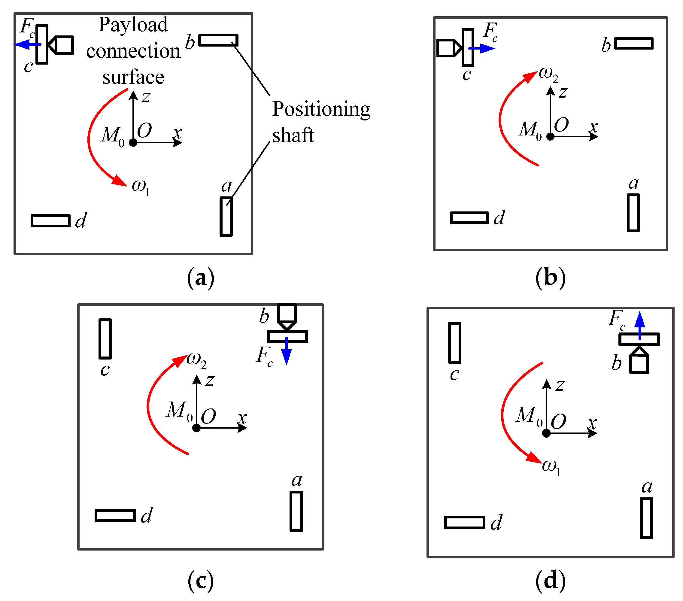
In the case where the directions of the four positioning shafts are determined, the corresponding direction of each capture hook needs to be further determined. In this scheme, the capture hook can only move in one plane, including rotation and translation, and if it is projected in the plane of the payload base, then it can only move in one direction. In the plane of the payload floor, if the capture hook in group c moves in the negative direction of the x-axis, the hook-frame contact force Fc will cause the payload to rotate counterclockwise around point O, and if the hook moves in the positive direction of the x-axis, the payload will be caused to rotate clockwise. Similarly, if the capture hook in group b moves in the negative direction of the z-axis, the payload will be forced to rotate clockwise around the point O, and if the hook in the positive direction of the z-axis, the payload will to rotate counterclockwise, as shown in Figure 19.
According to the influence of the movement direction of the capture hooks on the rotation direction of the payload during the capture process, it can be concluded that: For a set of active and passive catching lock assemblies where the movement direction of the capture hook is perpendicular to the axis of the catching frame, two directions can be selected, one of which will force the payload to rotate clockwise, and the other will force the payload to rotate counterclockwise. Since the movement of four sets of capture hooks are different, there are total movement arrangements. Therefore, to achieve the purpose of adjusting the attitude of the payload during the capture process, two capture hooks on a diagonal line are selected to rotate the payload clockwise, and two capture hooks on the other diagonal line to rotate the payload counterclockwise. Thus, group a cooperates with group c to make the payload rotate counterclockwise, and group b cooperates with group d to make the payload rotate clockwise, as shown in Figure 20. In this way, four sets of capture hooks work together to achieve the best payload and attitude adjustment effect during the capture process.
The positioning shaft of each passive end has two layout directions, parallel to either the x-axis or the z-axis. Thus, there are possible layouts for the four positioning shafts. Since the locking hook of each active end can only move along the positive and negative directions of the x-axis and the z-axis during capture, it will cause the payload to rotate after generating torque Mi. The number of possible layouts for the hooks also amounts to , and if all possible combinations for the hooks and positioning shafts are considered, 256 layouts would need to be analyzed. However, the classification can be simplified to reduce unnecessary work and improve simulation efficiency. The payload base plate has square symmetry, so the layout of the positioning shafts can be simplified into layouts, as shown in Figure 21.
The movement direction of the capture hook is perpendicular to the axial direction of the positioning shaft. When the positioning shaft is arranged in a certain direction, the direction of the contact torque for each group of hook frames is determined by the movement direction of the capture hook. If the contact force Fi for each group of hook frames is equal during capture, the contact torque for each group of hook frames is , and the magnitude of the torque has nothing to do with the arrangement direction of the positioning shafts or the movement direction of the capture hook. Thus, the movement direction of the capture hooks can also be simplified into layouts, as shown in Figure 22.
After simplification of the arrangement of the active and passive ends, the number of layouts for the capture and lock system can be simplified into possible arrangements.
2.3.2. Simulation Verification of Tolerance Capability for the Layout of Capture and Lock System
With the aim of determining the working characteristics of the distributed capture and lock system, a method for analyzing and verifying the tolerance capability of the capture and lock system is proposed, which is shown in Figure 23. The key steps are as follows:
- According to the boundary conditions of the structure size of the space payload and the working requirements of the capture and lock system, determine the simplest layout for the capture and lock system that will fully reflect the working conditions of the system;
- Determine the initial tolerance T0 and increase the tolerance by , then the system tolerance will be ;
- Convert the tolerance index Tm into a limit boundary pose that can be tested;
- Carry out the capture judgments for the limit boundary pose, and if all poses are successfully captured, set n = n+1, and continuously increase the tolerance for capture. If not all captures are successful, the system tolerance will be .
According to the boundary conditions for the shape and size of the payload and the working requirements of the capture and lock system, the initial tolerance was determined as and the incremental tolerance was . The iterative simulation tolerance capability analysis was carried out on system layouts, and the results are shown in Table 4.
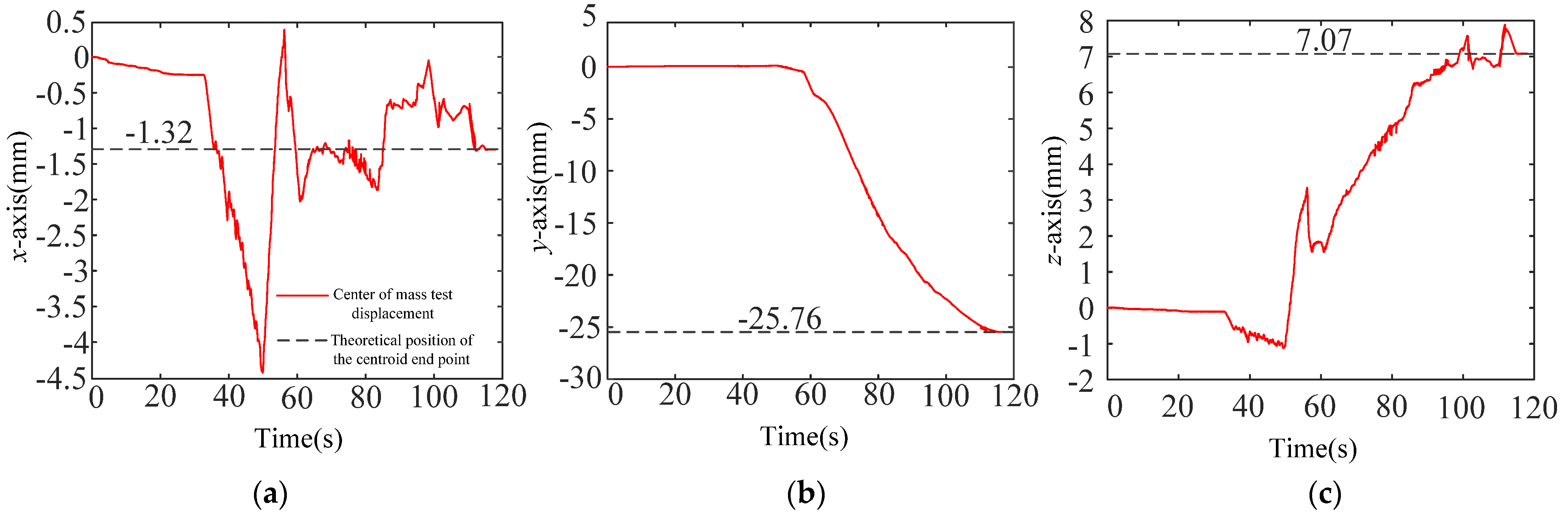
Among the 16 system layouts, the combination of a two-two diagonal orthogonal layout for the positioning shafts with a two-two moments unilateral balance for the movement direction of the capture hooks had a maximum tolerance of . The position change curve for the payload center of mass under the limit pose of this layout is shown in Figure 24.
3. Results
3.1. Development of a Space Payload Ground Capture Test System
Combined with the orthogonal distributed capture and lock system studied in this paper, a space payload ground capture test system was designed and developed. The capture test platform consists of an attitude adjustment system with six degrees of freedom, a simulated manipulator with seven degrees of freedom, a counterweight centering system with three degrees of freedom, a simulated payload, a six-dimensional force sensor, an orthogonally distributed capture and lock system, a motion capture system, and data acquisition. The composition of the control system is shown in Figure 25.
After the attitude adjustment system and the payload handle are connected and fixed by the spigot, the captured initial pose error for the simulated payload can be adjusted with the Oe point as the origin of the pose error. The simulated manipulator is composed of a simulated arm and a joint damper. During the capture process, the damper can generate damping that is inversely proportional to the motion speed, effectively simulating the manipulator in the follow-up damping control mode during the actual capture process. The counterweight centering system can change the spatial position of the suspension point by adjusting the bolts and can be used to accurately find the center of mass for the simulated payload when there is an error in the process of simulated payload processing and assembly. The counterweight method was used to simulate the microgravity environment in space, and the floating state of the payload in space was effectively simulated by suspension at the center of mass of the payload. To reduce the counterweight load and make test operation easy, a simulated payload was developed. The envelope size of the simulated payload is exactly the same as an actual payload, but the mass is smaller. The three-dimensional force sensor was installed at the end of the simulated manipulator. When the capture hook is in contact with the capture frame, the sensor will sense the force signal and feed it back to the control system, providing a basis for the selection of control strategies. The data acquisition and control system consisted of an upper computer, lower computer, and a control cabinet. The system was developed based on the xPC Target control module in MATLAB. The control cabinet is directly connected to the test system, collecting capture contact force, capture time, and other parameters to provide the basis for capture strategy selection, and sends out signals, such as capture hook speed, start and stop, etc., to execute the selected capture strategy.
During the capture test, a motion capture system was used to detect the pose of the payload. The motion capture system uses four cameras to monitor positional changes in the four targets, measure motion speed and track the centroid of the simulated payload. The test platform, camera layout, and target capture positions are shown in Figure 26. Before the motion capture system can be used, system calibration must be carried out. Through the calibration of the relative position of the camera, calibration of the horizontal plane, and calibration of the global coordinate system, position information can be collected. A target is pasted on key positions of the model, the surface of the target is then covered with a photosensitive material, and the camera determines the position of the target after receiving reflected light from the target. In fact, a single target point is identified as a line passing through the target point and perpendicular to the mirror of a single camera. If the target point pt coordinates are (xt, yt, zt), the normal vector perpendicular to the mirror of camera 1 is nt1 (ut1, vt1, wt1), then camera 1 identifies the target point pt as a straight line lt1:
The normal vector perpendicular to the mirror of camera 2 is nt2 (ut2, vt2, wt2), and camera 2 recognizes the target point pt as the straight line lt2:
The pt coordinates of the target points can be obtained by combining Equations (11) and (12), which is the principle for a motion capture system to identify the coordinates of a target point. To obtain the position data for the center of mass Ct of a rigid body, at least three target points that are not on the same line need to be pasted on the rigid body: pt1(xt1,yt1,zt1), pt2(xt2,yt2,zt2), and pt3(xt3,yt3,zt3). If the distances from the three target points to the centroid are dt1, dt2, and dt3, respectively, the Ct coordinates for the centroid of a rigid body can be obtained by solving the following equation:
By calculating the coordinates of the target point, the attitude data for a rigid body can be obtained, and the change in the position and attitude of the point of interest, such as the center of mass of a rigid body, can also be calculated.
In the space payload ground capture test system, it was necessary to measure changes in the position and attitude trajectory of the simulated payload center of mass. In theory, at least three target points and two cameras are required. To avoid the phenomenon of missing target images caused by the occlusion of platform components during the shooting process, four target points and four cameras were used. The target images captured by the four cameras and the positions of the four cameras are shown in Figure 27.
3.2. Experimental Verification of Capturing Tolerance Capability
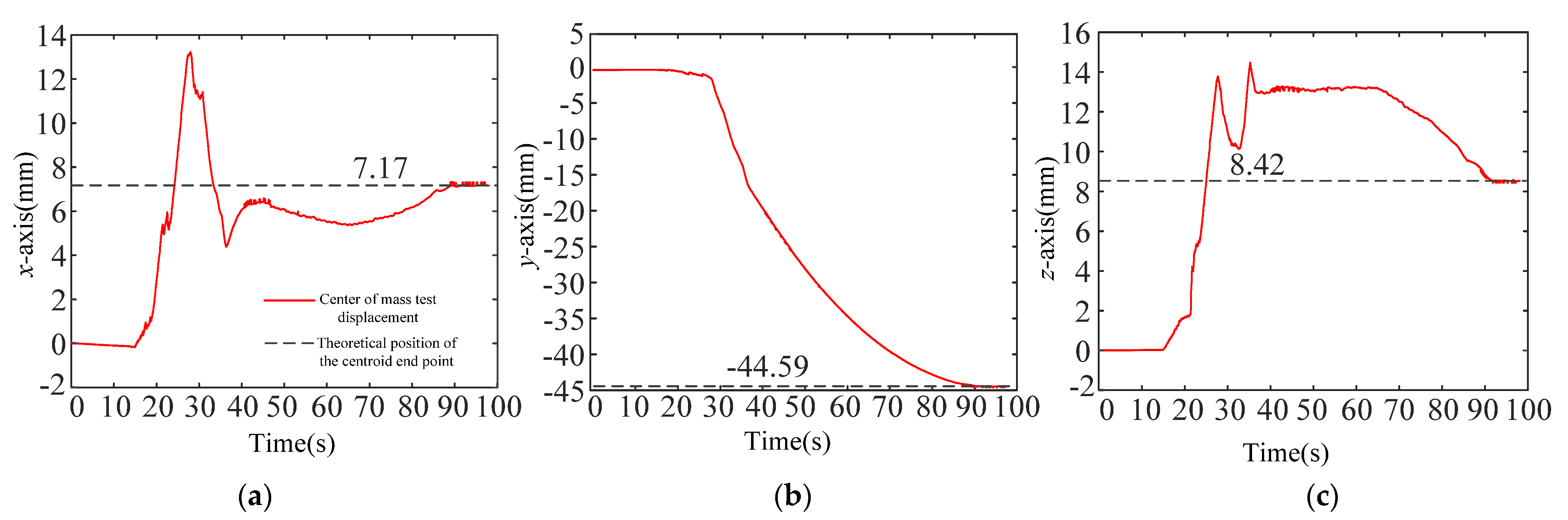
To verify the synchronous capture tolerance capability of the developed orthogonal distributed capture and lock system, the space payload ground capture test system was used to perform tolerance capability tests on the boundary poses of four types of typical boundary errors, as shown in Table 5.
Using the space payload ground capture test system and the motion capture system to carry out the synchronous capture tests, the trajectories for the center of mass of the simulated payload in the four groups are shown in Figure 28, Figure 29, Figure 30 and Figure 31. It was found that the displacement curves obtained by the synchronous capture test were constantly approaching the theoretical end position for the displacement of the center of mass, which proves that the tolerance capability of the capture and lock system had reached .
4. Discussion
In this paper, modular parameter design and analysis of a capture and lock mechanism was carried out, and a parameterized capture and lock mechanism unit with strong versatility and adaptability and a highly reliable capture and lock system layout was obtained. The system layout was simulated and verified by experiments, and the large-tolerance capturing capability of the system layout was verified, which is briefly summarized as follows:
- A multi-point over-positioning evaluation model was established, the positioning design of the capture and lock mechanism was carried out, and a positioning mechanism with an orthogonal layout was obtained, which created a foundation for designing the configuration of the capture and lock mechanism;
- Through the analysis of the payload attitude and the error domain for the passive end, the planning and design of the capture trajectory of the active end was completed, and the configuration of the passive end was obtained by comprehensively considering the optimal dynamic performance of the system. A mathematical model for the capture and lock mechanism was established, and the ideal trajectory parameters for the active end were obtained. Through the analysis of the capture trajectory curve, optimization of the configuration parameters for the capture lock system was completed;
- To improve payload attitude adjustment, the system positioning method was comprehensively considered, the layout design of the active end was carried out, and the system layout with the largest tolerance capacity and optimal attitude adjustment was obtained;
- A simulation was used to verify the layout tolerance capability of the capture lock system, a space payload ground capture test system was developed, and a system layout tolerance capability test was carried out to verify the large-tolerance capability of the developed capture system.
Author Contributions
Conceptualization, G.W.; methodology, Y.Y. and G.W.; software, J.W. and Y.Y.; validation, W.H.; formal analysis, G.X.; investigation, X.H.; resources, G.W.; data curation, Y.Y. and G.W.; writing—original draft preparation, Y.Y.; writing—review and editing, G.W. and Y.Y.; visualization, Y.Y.; supervision, G.W.; project administration, G.W.; funding acquisition, G.W. All authors have read and agreed to the published version of the manuscript.
Funding
This research was funded by the Youth Natural Science Foundation of Hebei Province, grant number E2021409025; the S & T Program of Hebei, grant number 21375414D; Scientific Research Project of Higher Education Institutions of Hebei Province, grant number QN2022123; and the Central Guidance on Local Science and Technology Development Fund of Hebei Province, grant number 226Z1803G.
Institutional Review Board Statement
Not applicable.
Informed Consent Statement
Not applicable.
Data Availability Statement
Not applicable.
Acknowledgments
The authors gratefully acknowledge the full support of the Langfang Municipal Science and Technology Program Self-financing Project, grant number 2021011068; the PhD research startup foundation of North China Institute of Aerospace Engineering, grant number BKY-2021-11; the Postgraduate Innovation Funding Project of North China Institute of Aerospace Engineering, grant numbers YKY-2021-22, YKY-2021-23; and Hebei Education Department innovative ability training support project for postgraduate students, CXZZSS2022133.
Conflicts of Interest
The authors declare no conflict of interest.
References
- Zhu, A.; Ai, H.; Chen, L. A Fuzzy Logic Reinforcement Learning Control with Spring-Damper Device for Space Robot Capturing Satellite. Appl. Sci. 2022, 12, 2662. [Google Scholar] [CrossRef]
- Carignan, C.; Scott, N.; Roderick, S. Hardware-in-the-loop simulation of satellite capture on a ground-based robotic testbed. In Proceedings of the International Symposium on Artificial Intelligence, Robotics and Automation in Space (i-SAIRAS), Montreal, QC, Canada, 17–19 July 2014; p. 6. [Google Scholar]
- Rekleitis, I.; Martin, E.; Rouleau, G.; L’Archevêque, R.; Parsa, K.; Dupuis, E. Autonomous capture of a tumbling satellite. J. Field Robot. 2007, 24, 275–296. [Google Scholar] [CrossRef]
- Kaiser, C.; Rank, P.; Krenn, R. Simulation of the docking phase for the SMART-OLEV satellite servicing mission. In Proceedings of the i-SAIRAS: International Symposium on Artificial Intelligence, Robotics and Automation in Space, Cologne, Germany, 25 February 2008; pp. 26–29. [Google Scholar]
- Huang, J.; Li, Z.; Huang, L.; Meng, B.; Han, X.; Pang, Y. Docking mechanism design and dynamic analysis for the GEO tumbling satellite. Assem. Autom. 2019, 39, 432–444. [Google Scholar] [CrossRef]
- Jaworski, J.; Dudek, L.; Wolski, M.; Mateja, A.; Wittels, P.; Labecki, M. Grippers for Launch Adapter Rings of Non-cooperative Satellites Capture for Active Debris Removal, Space Tug and On-Orbit Satellite Servicing Applications Holl. ASTRA ESTEC 2017. Available online: https://www.semanticscholar.org/paper/GRIPPERS-FOR-LAUNCH-ADAPTER-RINGS-OF-SATELLITES-FOR-Jaworski-Dudek/edd6822509bbc83b1be9640dfa840e1d39983576 (accessed on 12 May 2022).
- Rouleaut, G.; Martin, E.; Sharf, I. Trajectory Generation for Satellite Capture Using a Redundant Manipulator. In Romansy 16; Springer: Vienna, Austria, 2006; pp. 413–420. [Google Scholar]
- Wang, G.; Xie, Z.; Lu, Y.; Wang, J.; Wu, M.; Yang, F.; Jiang, S. Analysis method of the capture tolerance capability for an orthogonally distributed satellite capture device. IEEE Access 2019, 7, 55022–55034. [Google Scholar] [CrossRef]
- Wang, G.; Yang, F.; Jiang, S.; Yue, H.; Lu, Y.; Wu, M. Determination method of capture for an orthogonal distributed satellite capture device. IEEE Access 2018, 6, 61800–61811. [Google Scholar] [CrossRef]
- Wang, G.; Xie, Z.; Mu, X.; Li, S.; Yang, F.; Yue, H.; Jiang, S. Docking Strategy for a Space Station Container Docking Device Based on Adaptive Sensing. IEEE Access 2019, 7, 100867–100880. [Google Scholar] [CrossRef]
- Ma, Z.; Ma, O.; Shashikanth, B.N. Optimal approach to and alignment with a rotating rigid body for capture. J. Astronaut. Sci. 2007, 55, 407–419. [Google Scholar] [CrossRef]
- Wang, H.; Xie, Y. On the uniform positive definiteness of the estimated inertia for robot manipulators. IFAC Proc. Vol. 2011, 44, 4089–4094. [Google Scholar] [CrossRef] [Green Version]
- Wang, F.; Sun, F.; Liu, H. Space robot modeling and control considering the effect of orbital mechanics. In Proceedings of the 2006 1st International Symposium on Systems and Control in Aerospace and Astronautics, Harbin, China, 19–21 January 2006; Volume 6, p. 198. [Google Scholar]
- Rybus, T.; Seweryn, K.; Sasiadek, J.Z. Trajectory optimization of space manipulator with non-zero angular momentum during orbital capture maneuver. In Proceedings of the AIAA Guidance, Navigation, and Control Conference, San Diego, CA, USA, 4–8 January 2016; p. 0885. [Google Scholar]
- Xu, W.; Liu, Y.; Xu, Y. The coordinated motion planning of a dual-arm space robot for target capturing. Robotica 2012, 30, 755–771. [Google Scholar] [CrossRef]
- Tortopidis, I.; Papadopoulos, E. On point-to-point motion planning for underactuated space manipulator systems. Robot. Auton. Syst. 2007, 55, 122–131. [Google Scholar] [CrossRef]
- Aghili, F. Coordination control of a free-flying manipulator and its base attitude to capture and detumble a noncooperative satellite. In Proceedings of the 2009 IEEE/RSJ International Conference on Intelligent Robots and Systems, St. Louis, MO, USA, 10–15 October 2009; pp. 2365–2372. [Google Scholar]
- Piersigilli, P.; Sharf, I.; Misra, A.K. Reactionless capture of a satellite by a two degree-of-freedom manipulator. Acta Astronautica 2010, 66, 183–192. [Google Scholar] [CrossRef]
- Wang, G.; Yang, F.; Yue, H.; Jiang, S. Optimal layout method of distributed locking device of satellite based on plant root growth theory. Proc. Inst. Mech. Eng. Part G J. Aerosp. Eng. 2019, 233, 2802–2818. [Google Scholar] [CrossRef]
- Wang, G.; Yang, F.; Yue, H.; Jiang, S.; Wang, K. A new approach for design of a satellite modular reusable locking-release device. In Proceedings of the 2017 IEEE International Conference on Information and Automation (ICI(A), Macau, China, 18–20 July 2017; pp. 559–564. [Google Scholar]
- Lim, J.; Chung, J. Dynamic analysis of a tethered satellite system for space debris capture. Nonlinear Dyn. 2018, 94, 2391–2408. [Google Scholar] [CrossRef]
- Yoshida, K.; Dimitrov, D.; Nakanishi, H. On the capture of tumbling satellite by a space robot. In Proceedings of the 2006 IEEE/RSJ International Conference on Intelligent Robots and Systems, Beijing, China, 9–13 October 2006; pp. 4127–4132. [Google Scholar]
- Yoshida, K.; Nakanishi, H.; Ueno, H.; Inaba, N.; Nishimaki, T.; Oda, M. Dynamics, control and impedance matching for robotic capture of a non-cooperative satellite. Adv. Robot. 2004, 18, 175–198. [Google Scholar] [CrossRef]
Figure 1.
Schematic diagram of the space station material replacement task.

Figure 2.
Schematic diagram of the position and attitude error working conditions for the capture and lock system. (a) Working conditions of the capture and lock system; (b) schematic diagram of load pose error.
Figure 2.
Schematic diagram of the position and attitude error working conditions for the capture and lock system. (a) Working conditions of the capture and lock system; (b) schematic diagram of load pose error.

Figure 3.
Layout of the connection point for the capture and lock mechanism on the bottom of the payload.
Figure 3.
Layout of the connection point for the capture and lock mechanism on the bottom of the payload.

Figure 4.
Schematic diagram of a circular shaft-V-groove positioning arrangement. (a) Three-one orthogonal arrangement diagram; (b) two-two orthogonal arrangement diagram.
Figure 4.
Schematic diagram of a circular shaft-V-groove positioning arrangement. (a) Three-one orthogonal arrangement diagram; (b) two-two orthogonal arrangement diagram.

Figure 5.
Schematic diagram of positioning shaft and V-groove.

Figure 6.
Schematic diagram of the positioning shaft and V-groove layout.

Figure 7.
Capture frame configuration. (A: The top plate center of capture frame; B: The positioning shaft center of capture frame.)
Figure 7.
Capture frame configuration. (A: The top plate center of capture frame; B: The positioning shaft center of capture frame.)

Figure 8.
Schematic diagram of the payload coordinate system.

Figure 9.
Schematic diagram of capture frame error field. (a) Capture box cutaway view; (b) schematic diagram of the key point error field. (A: The top plate center of capture frame; B: The positioning shaft center of capture frame.)
Figure 9.
Schematic diagram of capture frame error field. (a) Capture box cutaway view; (b) schematic diagram of the key point error field. (A: The top plate center of capture frame; B: The positioning shaft center of capture frame.)

Figure 10.
Schematic diagram of the capture frame configuration.

Figure 11.
Schematic diagram of the ideal active end feature point trajectory. (A: The top plate center of capture frame; B: The positioning shaft center of capture frame.)
Figure 11.
Schematic diagram of the ideal active end feature point trajectory. (A: The top plate center of capture frame; B: The positioning shaft center of capture frame.)

Figure 12.
Linear track mechanisms. (a) Crank–slider mechanism (A, B, C: Hinge; B: Key point.); (b) Robert mechanism (A, B, C, D, M: Hinge; A, B, M: Key point.); (c) λ mechanism (A, B, C, D: Hinge; M: Key point.); (d) Watt mechanism (A, B, C, D: Hinge; M: Key point.).
Figure 12.
Linear track mechanisms. (a) Crank–slider mechanism (A, B, C: Hinge; B: Key point.); (b) Robert mechanism (A, B, C, D, M: Hinge; A, B, M: Key point.); (c) λ mechanism (A, B, C, D: Hinge; M: Key point.); (d) Watt mechanism (A, B, C, D: Hinge; M: Key point.).

Figure 13.
Curve track mechanisms. (a) Crank-rocker mechanism (A, B, C, D: Hinge; B: Key point.); (b) disc cam mechanism (A, B, C: Hinge; B: Key point.); (c) moving cam mechanism (A: Hinge; M: Key point.); (d) double-rocker mechanism (A, B, C, D: Hinge; B: Key point.).
Figure 13.
Curve track mechanisms. (a) Crank-rocker mechanism (A, B, C, D: Hinge; B: Key point.); (b) disc cam mechanism (A, B, C: Hinge; B: Key point.); (c) moving cam mechanism (A: Hinge; M: Key point.); (d) double-rocker mechanism (A, B, C, D: Hinge; B: Key point.).

Figure 14.
Schematic diagram of the capture and lock mechanism.

Figure 15.
Schematic diagram of the capture scheme (a) Released state; (b) locked state. 1, capture box; 2(the red dotted line), capture hook vertex trajectory; 3, positioning axis; 4, V-groove; 5, capture hook.
Figure 15.
Schematic diagram of the capture scheme (a) Released state; (b) locked state. 1, capture box; 2(the red dotted line), capture hook vertex trajectory; 3, positioning axis; 4, V-groove; 5, capture hook.

Figure 16.
Schematic diagram of model parameters and trajectory formation process. (a) Initial state; (b) end state of curve segment trajectory; (c) locked state.
Figure 16.
Schematic diagram of model parameters and trajectory formation process. (a) Initial state; (b) end state of curve segment trajectory; (c) locked state.

Figure 17.
Schematic diagram of the analysis of the influence of the trajectory parameters on the capture hook vertex. (a) Analysis of parameter a; (b) analysis of parameters b, c, d; (c) analysis of parameter e; (d) analysis of parameter f; (e) analysis of parameter g; (f)analysis of parameter R; (g) analysis of parameter r.


Figure 18.
Schematic diagram of the trajectory passing through the capture frame error field. (A: The top plate center of capture frame; B: The positioning shaft center of capture frame.)
Figure 18.
Schematic diagram of the trajectory passing through the capture frame error field. (A: The top plate center of capture frame; B: The positioning shaft center of capture frame.)

Figure 19.
Schematic diagram of the direction of the capture hook and the direction of rotation for the payload. (a) Group c capture hooks in the negative x-axis; (b) group c capture hooks in the positive x-axis; (c) group b capture hooks in the negative z-axis; (d) group d capture hooks in the positive z-axis.

Figure 20.
Schematic diagram of the orientation layout of the capture hooks.

Figure 21.
Simplified classification layout of the positioning axis. (a) Three-one orthogonal layout; (b) two-two diagonal orthogonal layout; (c) two-two unilateral orthogonal layout; (d) parallel layout.
Figure 21.
Simplified classification layout of the positioning axis. (a) Three-one orthogonal layout; (b) two-two diagonal orthogonal layout; (c) two-two unilateral orthogonal layout; (d) parallel layout.

Figure 22.
Simplified classification of capture hook motion direction (a) Two−two moments unilateral balance; (b) Two−two moments diagonal balance; (c) Three−one moments reversal; (d) Four moments equal.
Figure 22.
Simplified classification of capture hook motion direction (a) Two−two moments unilateral balance; (b) Two−two moments diagonal balance; (c) Three−one moments reversal; (d) Four moments equal.

Figure 23.
Tolerance capability analysis process for the capture and lock system.

Figure 24.
Variation curve for the position of the payload center of mass. (a) Variation curve for the position along the x-axis of the payload center of mass; (b) Variation curve for the position along the y-axis of the payload center of mass; (c) Variation curve for the position along the z-axis of the payload center of mass.

Figure 25.
Schematic diagram of the space payload ground capture test system.

Figure 26.
Space payload ground capture test system. 1, attitude adjustment system with six degrees of freedom; 2, six-dimensional force sensor; 3, simulated payload; 4, counterweight centering system with three degrees of freedom; 5, orthogonal distributed capture and lock system; 6, simulated manipulator with seven degrees of freedom; 7, target; 8, camera; 9, data acquisition and control system.

Figure 27.
Target image and the positions of four camera in the space payload ground capture test system.
Figure 27.
Target image and the positions of four camera in the space payload ground capture test system.

Figure 28.
The displacement of the center of mass of the captured test payload in the first boundary pose (see Table 5 for details). (a) The x-axis displacement of the center of mass of the captured test payload in the first boundary pose; (b) The y-axis displacement of the center of mass of the captured test payload in the first boundary pose; (c) The z-axis displacement of the center of mass of the captured test payload in the first boundary pose.

Figure 29.
The displacement of the center of mass of the captured test payload in the second boundary pose (see Table 5 for details). (a) The x-axis displacement of the center of mass of the captured test payload in the second boundary pose; (b) The y-axis displacement of the center of mass of the captured test payload in the second boundary pose; (c) The z-axis displacement of the center of mass of the captured test payload in the second boundary pose.

Figure 30.
The displacement of the center of mass of the captured test payload in the third boundary pose (see Table 5 for details). (a) The x-axis displacement of the center of mass of the captured test payload in the third boundary pose; (b) The y-axis displacement of the center of mass of the captured test payload in the third boundary pose; (c) The z-axis displacement of the center of mass of the captured test payload in the third boundary pose.

Figure 31.
The displacement of the center of mass of the captured test payload in the fourth boundary pose (see Table 5 for details). (a) The x-axis displacement of the center of mass of the captured test payload in the fourth boundary pose; (b) The y-axis displacement of the center of mass of the captured test payload in the fourth boundary pose; (c) The z-axis displacement of the center of mass of the captured test payload in the fourth boundary pose.


Table 1.
Summary of common positioning methods.
| Serial Number | Positioning Form | Positioning Piece (a) | Positioning Piece (b) | Positioning Diagram | Restricted Degrees of Freedom | |
|---|---|---|---|---|---|---|
| 1 | Point positioning | Support nails | Flat piece |  | One movement degree of freedom | |
| 2 | Line positioning | Linear positioning | Long support plate | Flat piece |  | One movement degree of freedom and one rotational degree of freedom |
| Curve positioning | Taper pin | Cylinder |  | Two movement degrees of freedom | ||
| V-groove | Circular shaft |  | Two movement degrees of freedom and two rotational degrees of freedom | |||
| 3 | Face positioning | Plane positioning | Support plate | Flat piece |  | One movement degree of freedom and two rotational degrees of freedom |
| Rectangular pin | Rectangular tube |  | Two movement degrees of freedom and three rotational degrees of freedom | |||
| V-groove | V-block |  | ||||
| Surface positioning | Round pin | Cylinder |  | Two movement degrees of freedom and two rotational degrees of freedom | ||
| Circular cone | Tapered hole |  | Three movement degrees of freedom and two rotational degrees of freedom | |||
Table 2.
Three positioning methods to evaluate the key parameters of the model.
| Positioning Method | C1 | C2 | C2l | C2k | C3 | C3l | C3k | C4 | C4l | C4k | C | |
|---|---|---|---|---|---|---|---|---|---|---|---|---|
| Circular shaft-V-groove | Three-one orthogonal | 4 | 4 | 0 | 0 | 4 | 1 | 1 | 4 | 1 | 1 | 10 |
| Two-two orthogonal | 4 | 4 | 0 | 0 | 4 | 2 | 2 | 4 | 0 | 0 | 10 | |
| V-block-V-groove | Three-one orthogonal | 5 | 5 | 0 | 0 | 5 | 0 | 0 | 5 | 1 | 1 | 14 |
| Two-two orthogonal | 5 | 5 | 0 | 0 | 5 | 1 | 1 | 5 | 0 | 0 | 14 | |
| Circular cone-tapered hole | 5 | 5 | 1 | 1 | 5 | 0 | 0 | 5 | 0 | 0 | 14 | |
Table 3.
List of values for the parameters of the capture and lock mechanism.
| Parameter | a/mm | b/mm | c/mm | d/mm | e/mm | f/mm | g/mm | R/mm | r/mm |
|---|---|---|---|---|---|---|---|---|---|
| Value | 37 | 15 | 20 | 25 | 33 | 92 | 30 | 10 | 4 |
Table 4.
Layout tolerance capability of 16 capture and lock systems (measured in mm).
| Three-One Orthogonal Layout | Two-Two Diagonal Orthogonal Layout | Two-Two Unilateral Orthogonal Layout | Parallel Layout | |
|---|---|---|---|---|
| Two-two moments unilateral balance | ||||
| Two-two moments diagonal balance | ||||
| Three-one moments reversal | ||||
| Four moments equal |
Table 5.
Four types of typical boundary pose errors.
| Boundary Pose | x/mm | y/mm | z/mm | |||
|---|---|---|---|---|---|---|
| P1 | 10 | −10 | 10 | 1 | −1 | −1 |
| P2 | −10 | 10 | 10 | 1 | 1 | −1 |
| P3 | 10 | 10 | −10 | −1 | −1 | 1 |
| P4 | 10 | 10 | 10 | −1 | 1 | −1 |
Publisher’s Note: MDPI stays neutral with regard to jurisdictional claims in published maps and institutional affiliations. |
© 2022 by the authors. Licensee MDPI, Basel, Switzerland. This article is an open access article distributed under the terms and conditions of the Creative Commons Attribution (CC BY) license (https://creativecommons.org/licenses/by/4.0/).
Share and Cite
MDPI and ACS Style
Wang, G.; Yao, Y.; Wang, J.; Huo, W.; Xu, G.; Hu, X. Layout Design and Verification of a Space Payload Distributed Capture and Lock System. Aerospace 2022, 9, 345. https://0-doi-org.brum.beds.ac.uk/10.3390/aerospace9070345
AMA Style
Wang G, Yao Y, Wang J, Huo W, Xu G, Hu X. Layout Design and Verification of a Space Payload Distributed Capture and Lock System. Aerospace. 2022; 9(7):345. https://0-doi-org.brum.beds.ac.uk/10.3390/aerospace9070345
Chicago/Turabian StyleWang, Gang, Yimeng Yao, Jingtian Wang, Weiye Huo, Guosheng Xu, and Xi Hu. 2022. "Layout Design and Verification of a Space Payload Distributed Capture and Lock System" Aerospace 9, no. 7: 345. https://0-doi-org.brum.beds.ac.uk/10.3390/aerospace9070345
Note that from the first issue of 2016, this journal uses article numbers instead of page numbers. See further details here.