
Towards Money Market in General Equilibrium Framework


Faculty of Finance, The University of Danang—University of Economics, 71 Ngu Hanh Son St., Da Nang 550000, Vietnam
Int. J. Financial Stud. 2022, 10(1), 12; https://0-doi-org.brum.beds.ac.uk/10.3390/ijfs10010012
Submission received: 30 December 2021
/
Revised: 31 January 2022
/
Accepted: 5 February 2022
/
Published: 10 February 2022
Abstract
:This paper aims to integrate the money market into the structure of the economy. The microfoundation is the starting point to define the money market and the general equilibrium mechanism of the economy. On this basis, this research seeks a linking mechanism of the money market with economic activity in the general equilibrium framework. The relationships between money supply and national outcome, inflation, and price level are studied in three cases: full-employment equilibrium economy, steady-state equilibrium economy, and sticky-price equilibrium economy. The research result explains the interrelation and transmission mechanism between the money market and the general equilibrium of the economy. The paper provides the theoretical foundation for further research on the money market and monetary policies towards economic growth and macroeconomic stability.
JEL codes:
D01; D50; E40; E521. Introduction
The money market is an inseparable part of the structure of the economy. Accordingly, monetary policy is always associated with economic activities in which the role of money is emphasized in explaining economic fluctuations and inflation (Tavlas 1981). Therefore, the importance of the money market to the economy is the central topic in economic ideology and theory. The theory of money has developed with two contrasting views concerning the importance of money and monetary policy (Friedman 1956): the Fisherian view emphasizes controlling the quantity of money through the monetary policy, and the Keynesian view emphasizes aggregate demand through fiscal policy. The views on monetary instruments and policies that influence economic growth, inflation, and employment have been the subject of debate in theory and practice throughout the past century (Friedman 1968). Thus, the role of money and the transmission channel of monetary policy are rehabilitated (Adrian and Shin 2009).
The question in the monetary analysis debate is whether the quantity of money is exogenous (determined by money authorities) or endogenous (determined by economic activities). The Fisherian view relies on the classical quantity theory of money, in which monetarists argued that money is neutral in the long term and should also be in the short term. Changes in the general price level were linked to proportionate changes in the money supply (Fisher 1911). The Keynesian view relies on Keynes’s macroeconomic theory, in which money has real effects both in the long term and in the short term (Gaffard 2018). Keynes’s revolutionary contribution to economics lies in the theory of effective demand (Keynes 1930), in which money demand relies upon the national outcome determined by the IS-LM model (Hicks 1937; Hansen 1953). However, the IS-LM model was weak and unreliable due to a lack of microfoundations for general equilibrium. Meanwhile, the classical theory of general equilibrium (Walras 1874; Arrow and Debreu 1954) has not been conducted the money market in the general equilibrium models. According to Lucas (1972), the monetary system utilities the assumption of nominal price stickiness and embodies the framework of general equilibrium. Therefore, the new neoclassical synthesis combined neoclassical economics and Keynesian macroeconomics to provide microfoundations for dynamic stochastic general equilibrium. However, the dynamic stochastic general equilibrium (DSGE) model still fails to incorporate critical aspects of economic behavior and the financial sector to predict or respond to a financial crisis (Blanchard 2016; Stiglitz 2018).
Although many monetary theories and models have been developed for monetary policy analysis in economic development, the underlying monetary theories are deficient with solid foundations in linking the money market with economic activities. For these reasons, this paper integrates the money market into the general equilibrium framework. There are specific objectives that are carried out in this research. First, the monetary theory is developed upon the quality theory of money, Keynesian macroeconomic theory, and classical theory of general equilibrium. Second, the research develops microfoundations that are the key to explaining the market behaviors and general equilibrium mechanism. Last, the linking mechanism between the money market and economic activities is conducted under three typical cases: full-employment equilibrium economy, steady-state equilibrium economy, and sticky-price equilibrium economy.
2. Literature Review
Classical monetary theory is well-known as the quantity theory of money (Fisher 1911). The quantity theory of money emphasizes the role of money supply, assuming that the velocity of money and the national outcome are constant. The quantity theory of money argues that increasing the quantity of money will increase the price with the same proportion. However, the classical theory of money has not addressed the tradeoff between inflation and national outcome. Pigou (1917) emphasized the Marshallian view on money demand and the Fisherian view on the money supply, which was formulated in terms of the velocity of money circulation. Nevertheless, there seems to be one basic proposition characterizing the quantity theory of money. The money supply exogenously engineered by the monetary authorities has the long-run effect on a change in the price level (and other nominal variables) of the same proportion as the money stock, but no change in any real variables (McCallum and Nelson 2010). Monetarists (Friedman and Schwartz 1965; Friedman 1968) argued that an increase in the quantity of money will increase real GDP in the short run, but that money is neutral in the long run. However, the quantity theory of money is criticized by the assumption of a constant velocity of money (Mishkin 2001) and the neutrality of money in the long run (Evans 1996).
The Keynesian monetary theory emphasizes the money demand stemming from economic activities and the role of fiscal policy in promoting economic growth. Liquidity preference theory combines money demand (liquidity preference) with the money supply by central banks to determine the equilibrium interest rate (Keynes 1936). An increase in the money supply that lowers the interest rate positively affects the marginal efficiency of capital. This will promote the expansion of economic activities and increase the national outcome. In addition, Keynes was skeptical about the effectiveness of monetary policy when the economy is in a liquidity trap and because of uncertainty in the financial markets (Twinoburyo and Odhiambo 2018). The IS-LM model (Hicks 1937; Hansen 1953) explains the general equilibrium mechanism between the commodity market and money market through the intersection of the investment-savings (IS) and liquidity preference—money supply (LM). However, the IS-LM model lacks the precision and realism to be a useful prescription tool for economic policy. In both classical and Keynesian monetary theories, the assumption of exogenous money supply has been challenged and discarded in subsequent and modern theories (Romer 2006).
In recent literature, the modern monetary theory attempts to deal with the monetary-fiscal conflict based on practical experience in monetary and fiscal policies. Compared with the mainstream monetary theory, the modern monetary theory has contrasting views in funding government spending, achieving full employment, setting interest rates, and controlling inflation rates. According to modern monetary theory, the government can create money funded by the central bank for government spending in pursuit of socio-economic goals. Therefore, modern monetary policy is suitable for an economy with low inflation and high unemployment. In addition, the government can reduce government spending and raise taxes only if the economy has an inflationary problem. However, economic researchers believe that modern monetary theory’s monetary and fiscal policies can lead to high inflation, even hyperinflation, when the economy is in full employment. Moreover, since the modern monetary theory does not explain the interest rate mechanism and the relationship of money supply and money demand with economic activities, the modern monetary theory lacks a theoretical foundation for monetary policies and fiscal policy (Palley 2015).
The classical monetary theory lays the groundwork for developing new classical models (Goodfriend and King 1997; Palley 2007), in which the monetary policy does not affect real GDP according to the rational expectations hypothesis and real business cycle theory. Meanwhile, new Keynesian models assume that prices are rigid to fiscal or monetary policy (Goodfriend and King 1997). Meanwhile, the new consensus model is the product of the new classical model (rational expectations and real business cycles) and the new Keynesian model (price stickiness). The new consensus model suggests that monetary policy focuses on short-run output stabilization and long-run price stability (Fontana and Palacio-Vera 2007). In fact, monetary theories have been challenged on the grounds of the velocity of money and the instability of the money demand function (White 2013). Moreover, the underlying monetary models are the absence of money, exchange rate roles, inadequate treatment of markets (financial, labor, capital markets) (Arestis and Sawyer 2008).
Recently, monetary policy has been addressed in the general equilibrium framework (Woodford 2005; Christiano et al. 2010) through the monetary policy rules (the Taylor rule, Friedman’s k-percent rule, and other interest targeting rules). However, the rule-based approaches are only suitable under certain circumstances. The lack of a theoretical foundation has resulted in limitations in the monetary theories and models. Therefore, monetary policies and rules pursued for a long time with potential risks will lead to stagnation phenomena and economic crisis. Monetary theory built on solid microfoundations is the key to understanding the nature of the money market. The linkage of the money market within the general equilibrium framework is the basis for explaining the transmission mechanism and the role of monetary and fiscal policy on economic growth and stability.
3. General Equilibrium
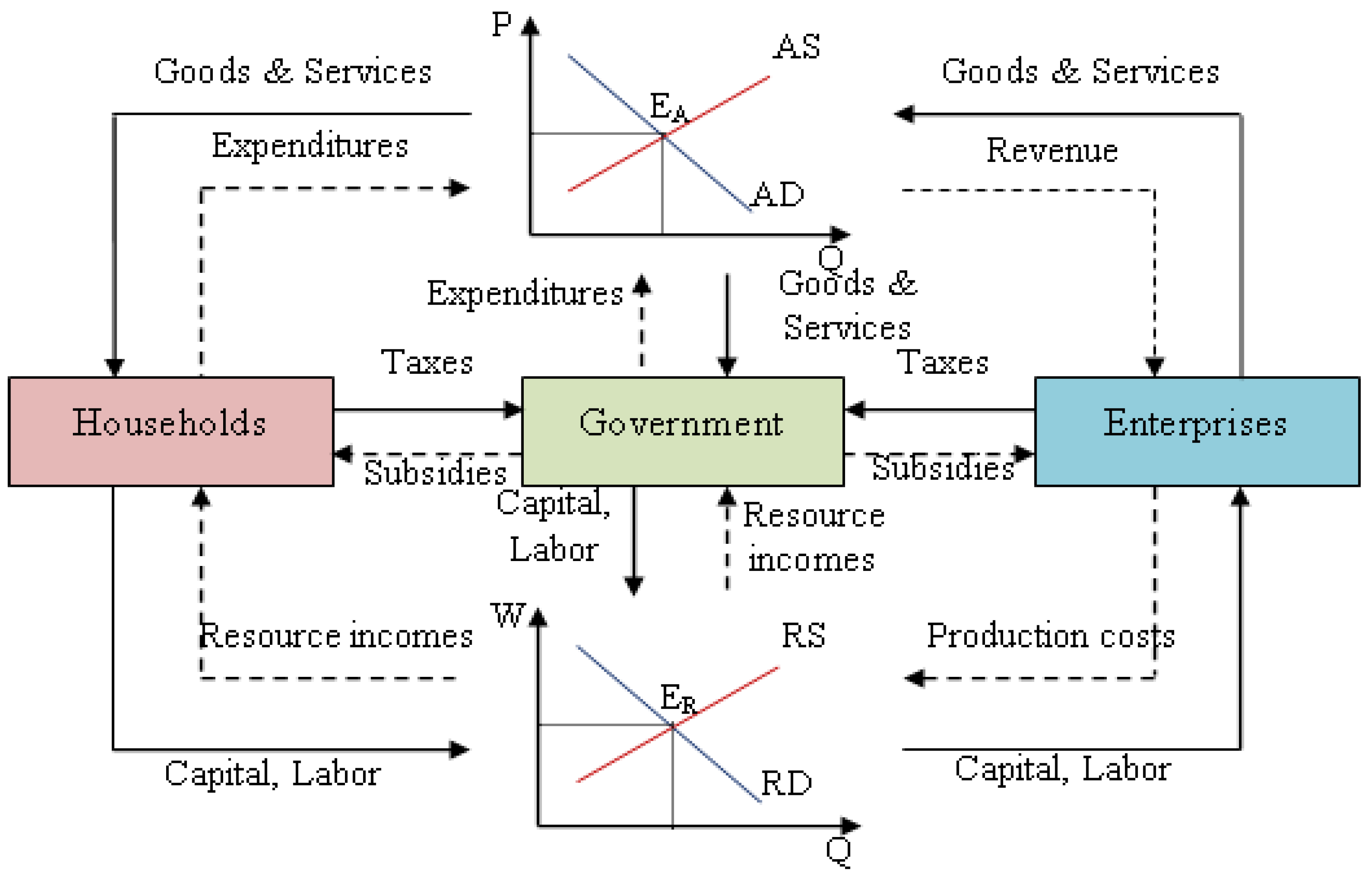
The general equilibrium theory describes the interaction mechanism between economic actors (household, business, government) in the markets (commodity market, resource market). Therefore, the structure of the economy is the starting point for building a general equilibrium theory. Figure 1 illustrates the simple economic system in which the national economy assumes no taxes and subsidies, no international trade and investment with the rest of the world. In such an economy, the aggregate commodity demand (AD) presents the relationship between the average commodity price (pAD) and the total quantity demanded (Q) in the economy. From the GDP formula (Trinh 2018), the aggregate commodity demand (AD) includes household spending , government spending , and enterprise investment rewritten as follows:
where is the total production quantity of the economy and is the average commodity price in the economy.
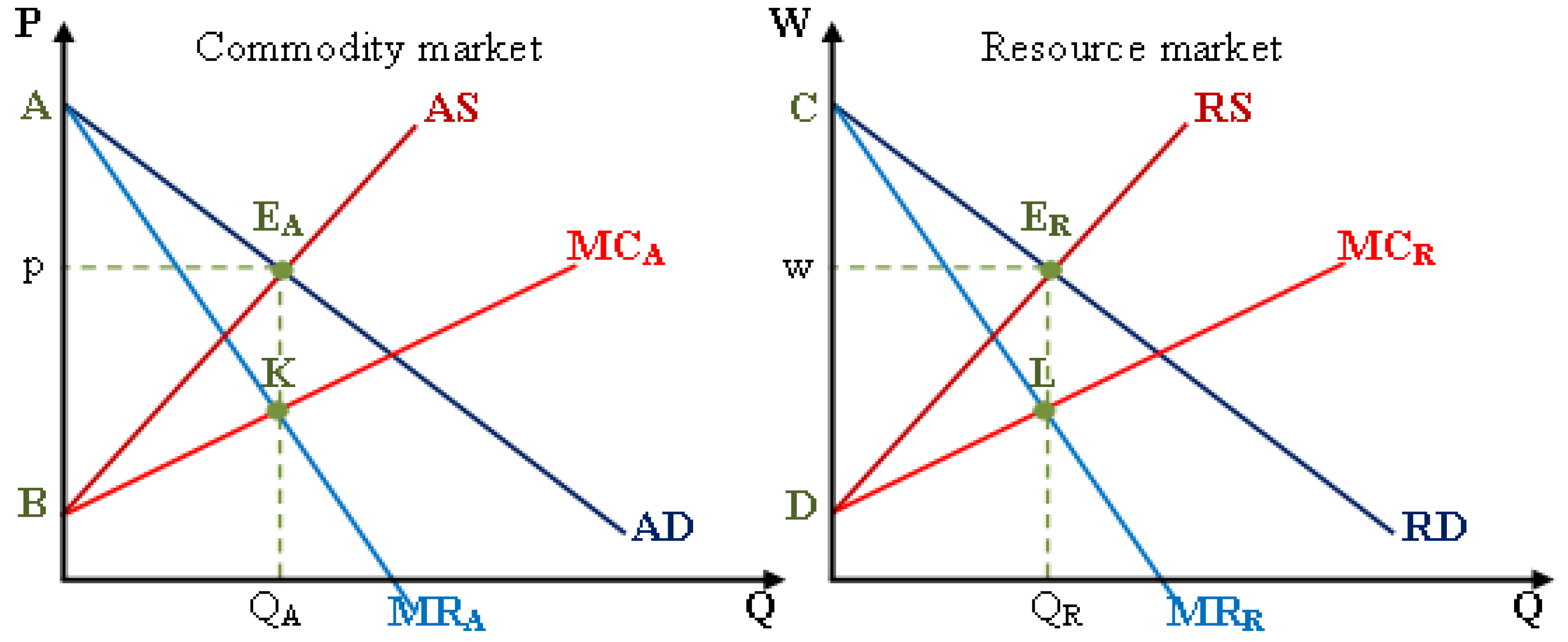
The aggregate commodity supply (AS) is determined on the basis of the relationship between the market equilibrium and the marginal equilibrium in the commodity market. The aggregate commodity supply (AS) intersects the aggregate commodity demand (AD) at the equilibrium quantity (QA), where total marginal revenue (MRA) is equal to total marginal cost (MCA) in the commodity market (Trinh 2018, 2019) as illustrated in Figure 2. Based on this relationship, the aggregate commodity supply (AS) is determined as follows:
where is the first derivative of the aggregate commodity demand function is determined upon the first derivative of the total cost function (TCA) in the commodity market.
The relationship between total production cost (TCA) in the commodity market and total revenue in the resource market is illustrated as follows:
where is the average resource price and Q is the total production quantity in the economy.
Substituting into Equation (2), the aggregate commodity supply function is rewritten as follows:
The aggregate resource supply (RS) is determined by the relationship between the market equilibrium and the marginal equilibrium in the resource market. The market equilibrium of the resource at QR where total marginal revenue (MRR) is equal to the total marginal cost (MCR) in the resource market as illustrated in Figure 2. At this equilibrium quantity, the aggregate resource supply (RS) will intersect the aggregate resource demand (RD) in the resource market. Based on this relationship, the aggregate resource supply (RS) is determined as follows:
where is the first derivative of the aggregate resource demand function is determined on the first derivative of the total cost function (TCR) in the resource market. The relationship between the total cost (TCR) in the resource market and the total revenue in the commodity market is illustrated as follows:
Replacing into Equation (6), the aggregate resource supply function (RS) is rewritten as follows:
The aggregate supply is identified from the relation between market and marginal equilibrium, relying on its aggregate demand and marginal cost (Trinh 2020, 2021). From this base, the total economic surplus in the commodity market is the area AKB (equals the area AEAB). Similarly, the total economic surplus in the resource market is the area CLD (equals the area CERD), as illustrated in Figure 2.
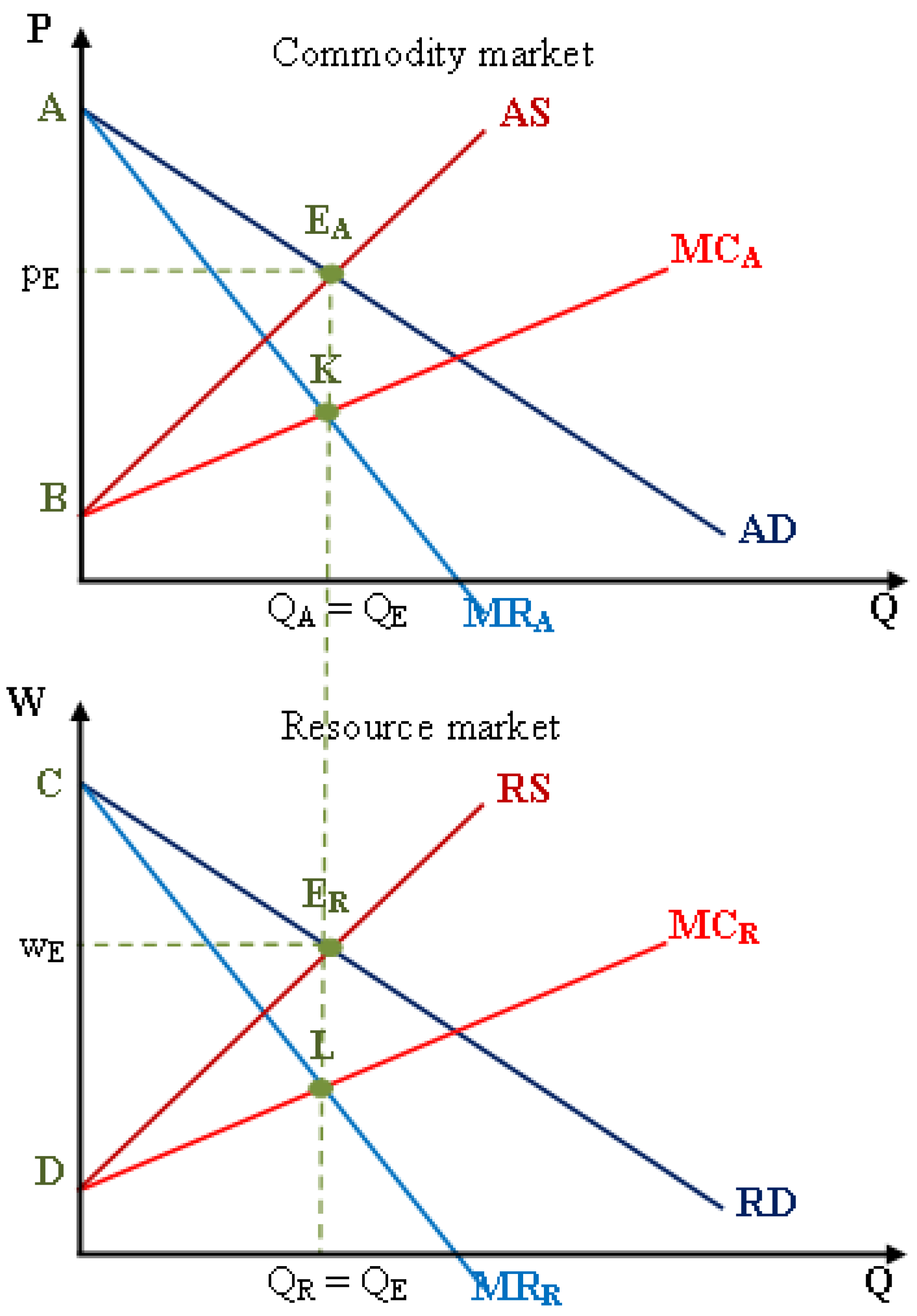
The general equilibrium of the economy occurs only when the equilibrium quantity of the commodity market (QA) equals the equilibrium quantity of the resource market (QR) as illustrated in Figure 3. When the equilibrium quantity of the commodity market (QA) is greater than (or less than) the equilibrium quantity of the resource market (QR), the economy is in general disequilibrium status. The concept of the economic surplus is the crucial basis of behavior analysis and decision-making of economic actors in the markets. While the market equilibrium represents each economic actor’s partial (individual) rational choice, the general equilibrium represents economic actors’ general (cooperative) rational choice. When the economy reaches general equilibrium at the equilibrium quantity (QE), the average commodity price is determined at pE, and the average resource cost is determined at wE, as illustrated in Figure 3. Since the total economic surplus (economic welfare) is the sum of AKB and CLD, the economic welfare (total economic surplus in the commodity and resource markets) is maximized in the general equilibrium economy.
4. Money Market
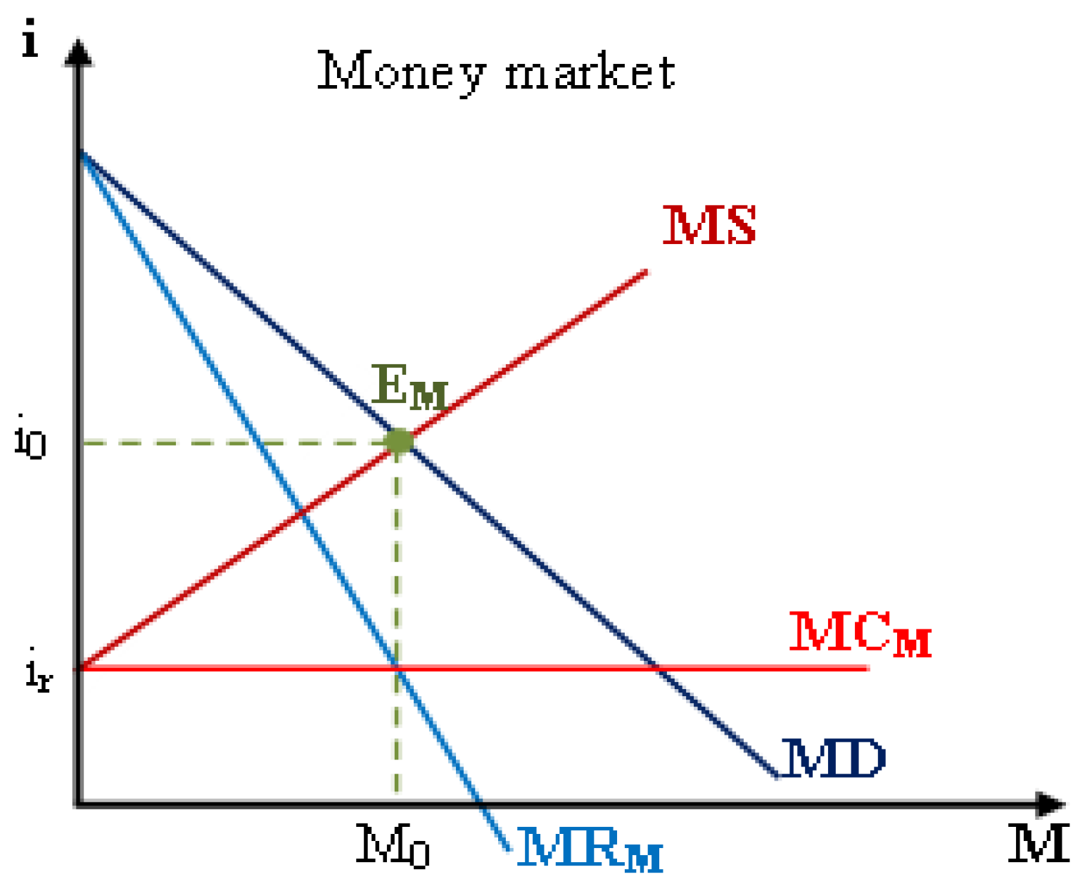
The money market presents the relationship between the demand and supply of money. The demand for money represents the relationship between the nominal interest rate (the price of money) and the quantity demanded of money over a given period. The money supply presents the relationship between the nominal interest rate (the price of money) and the quantity supplied of money over a given period. The equilibrium of the money market occurs at the nominal interest rate (equilibrium price of money), where the quantity demanded of money is equal to the quantity supplied of money, as illustrated in Figure 4.
Total revenue (TRM) and marginal revenue (MRM) on the money market are determined as follows:
where is the money demand function and is the first derivative of the money demand function.
Since the nominal interest rate (iD) is defined as the point where the money supply intersects the money demand, the real interest rate (ir) is defined as the marginal cost of money (MCM). This definition is relevant to Fisher’s monetary theory (Fisher 1911, 1930) and empirical research (Fama 1975), in which the real interest rate is constant through time and approximately equal to the nominal interest rate minus the expected inflation rate.
Figure 4 illustrates the relationship between market equilibrium and marginal equilibrium in the money market. At the equilibrium money quantity (ME), where the money demand curve intersects the money supply curve , the marginal revenue of money (MRM) is also equal to the marginal cost of money (MCM).
From Equations (11) and (12), the money supply function is determined at and replacing by as follows:
From Equation (13), the money supply function relies on the money demand and marginal cost of money .
According to the standard Fisher hypothesis (Fisher 1930), the nominal interest rate (i) relies on the real interest rate (ir) and the inflation rate (f) as in Equation (14), in which the real interest rate is estimated as return on treasury bills that seems to be constant through time. Meanwhile, the inverted Fisher hypothesis (Carmichael and Stebbing 1983) states the constancy of the nominal interest rate relative to inflation and the inverse correlation between inflation and the real interest rate.
According to the Fisherian approach, the nominal interest rate is defined as the real interest rate plus the inflation rate .
From Equations (13) and (14), the relationship between inflation and the money demand and the money quantity supplied is as follows:
The quantity theory of money (Fisher 1911) expresses the relationship between the quantity of money (M) and the nominal national income (Y) as follows:
where V is the velocity of money. The nominal national income (Y) is determined by the price (p) and quantity (Q) when the economy is in the general equilibrium status. Figure 5 illustrates the relationship between the money market and the commodity market in general equilibrium status. From Equation (16), the formula of money quantity (M) is computed as follows:
Equation (17) reveals that the money supply (M) depends on the nominal national income (Y = p × Q) and the velocity of money (V). The nominal national income (Y) derives from investments in both real assets and financial assets. Also, the velocity of money (the money turnover) must be estimated upon economic activities associated with the real and financial assets.
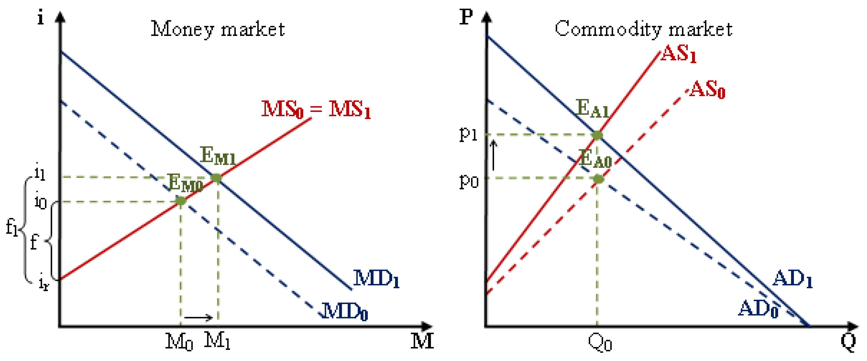
In the case of the full-employment equilibrium economy, an increase in the money supplied (M) will increase the nominal interest rate (i) and inflation (f), respectively. From the formulation of money quantity (17), when Q and V are constant, the growth rate of money (g) in the money market will correspond to the growth rate of the price level in the commodity market, as illustrated in Figure 6.
Equation (19) is developed upon the standard Fisher hypothesis. However, the inverted Fisher hypothesis may be concerned as the structure of the money market is extended with the bond market and regulations on interest rates.
In such a case, the price level in the economy and inflation in the money market have the same growth rates. This growth rate leads to an increase in the nominal GDP but has no impact on economic activity and the economy’s structure. This full-employment monetary model is relevant to the classical theory of money in explaining that monetary policies do not affect the real GDP. Thus, the monetary policies focus on money demand as the main driving force that affects the interest rate in the money market.
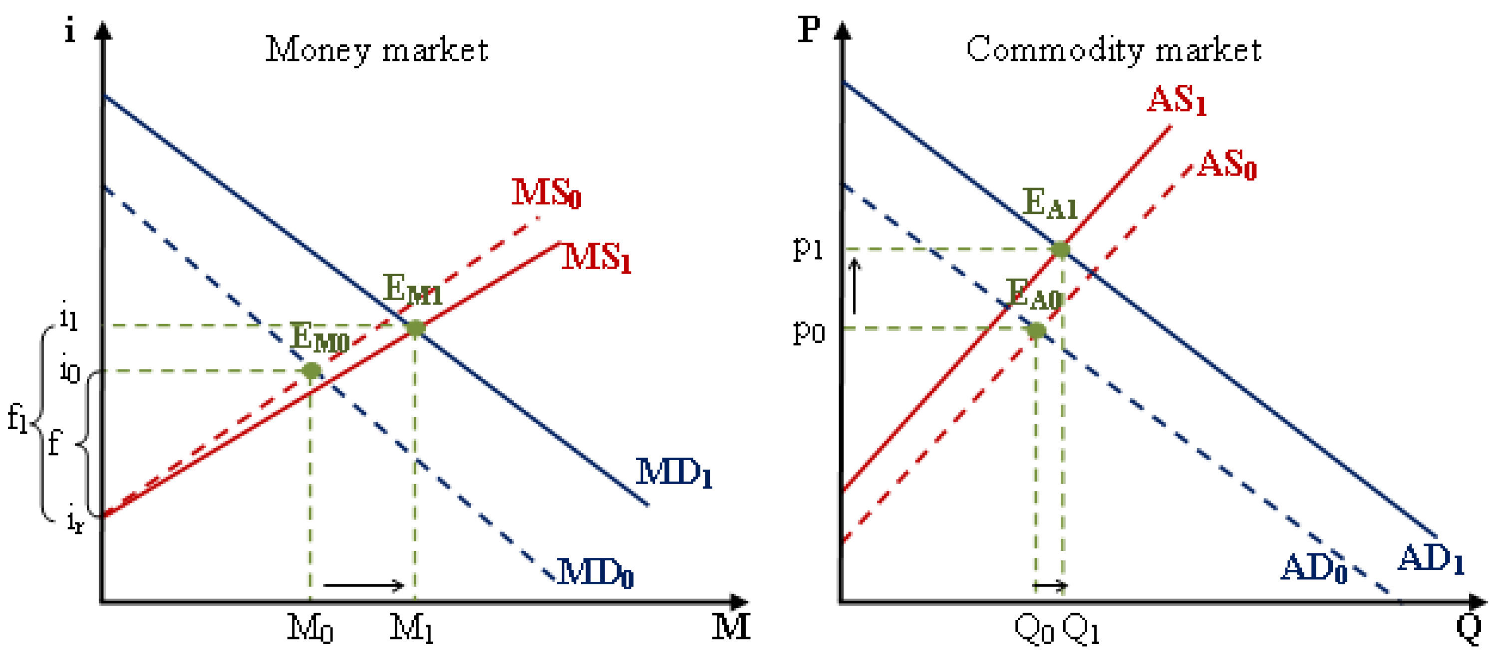
In the case of the steady-state equilibrium economy, the economic growth responds with the market scale in which there are increases in the quantity (Q) and the price (p) at the same rate as shown in Figure 7. Then, the money supplied (M1) in the case of the steady-state equilibrium is determined as follows:
From Equation (20), the monetary model may extend with the real business cycle hypothesis, in which the levels of price and quantity increase with different growth rates, but the price level in the economy and inflation in the money market are always the same growth rate as in Equation (21).
Equation (20) may be extended and applied for the real economy under economic policies (or economic shocks) in which the growth rate of the quantity and price are not the same. However, the growth rates of inflation and the price level are always the same as in Equation (21).
When the equilibrium quantity increases from Q→Q1 and the equilibrium price increases from p→p1, the money quantity increases from M→M1. The aggregate demand and aggregate supply increase at the same rate (g) to reach the steady-state equilibrium status. Assuming the real interest rate (or marginal cost of money) remains constant, the money supply function (iS) and the money demand function (iD) are illustrated in Figure 7.
The steady-state monetary model is relevant with the classical theory of general equilibrium and the new classical model with rational expectations hypothesis, in which the levels of price and quantity increase with the same growth rate as the nominal GDP. The monetary policy focuses on both monetary demand and money supply in which the money supply responds to changes in nominal interest rate.
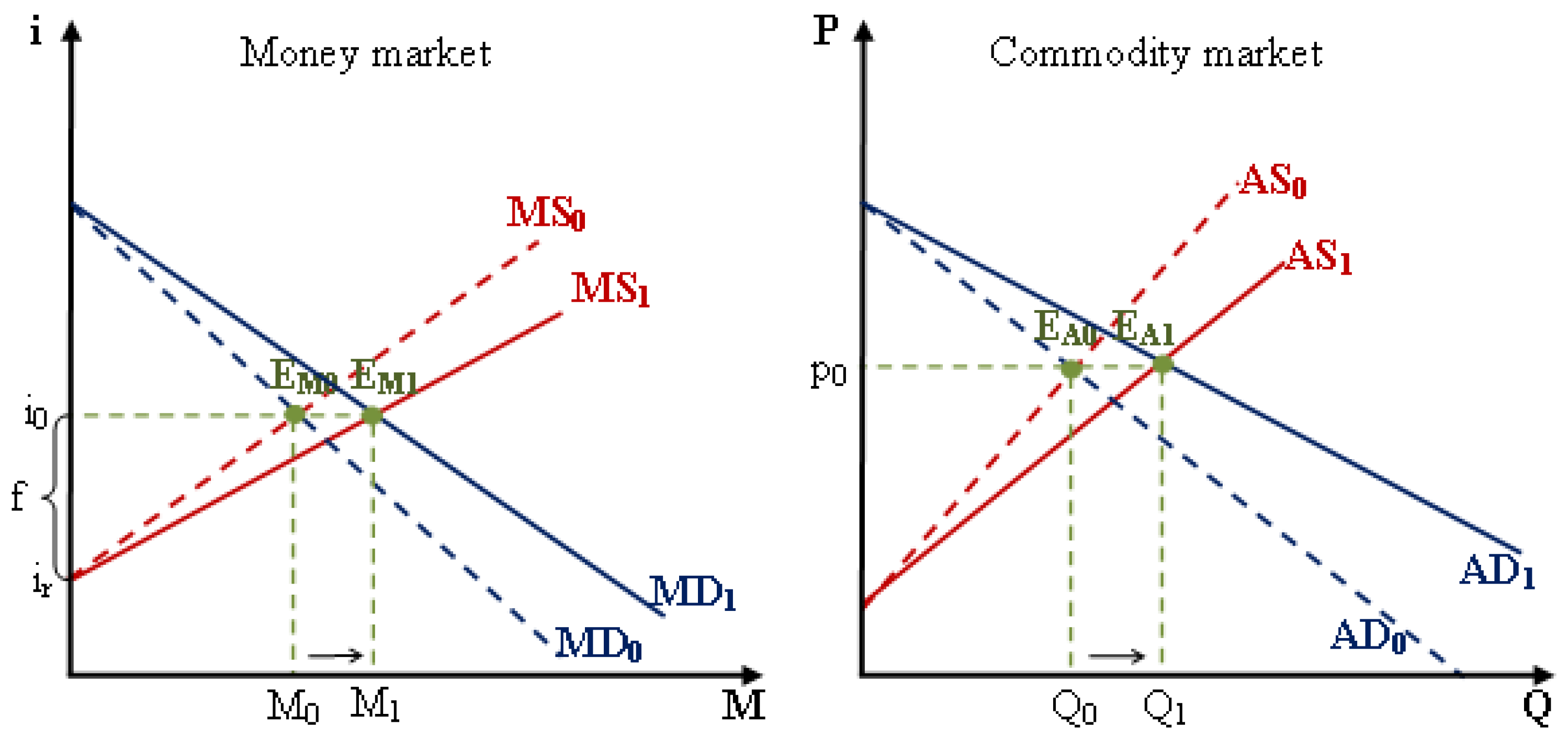
In the case of the sticky-price equilibrium economy, the economic growth (nominal national income) is due to an increase in the quantity (Q1 = Q × (1 + g)) and no increase in the price. Then, the money supplied (M1) increases with the growth rate of the equilibrium quantity of the economy as follows:
When the equilibrium quantity increases from Q→Q1 and the equilibrium price remains constant p = p1, the money quantity increases from M→M1 while the nominal interest rate (i) and inflation rate (f) remain constant for the general equilibrium economy under the sticky price. The demand and supply of money are illustrated in Figure 8.
The sticky-price monetary model is relevant with the Keynesian monetary theory and the new Keynesian models with nominal rigidity hypothesis, in which the price and wage are rigid to changes in fiscal and monetary policies. Thus, the sticky-price monetary policies focus on money demand and money supply to maintain a stable interest rate.
These monetary models are the extreme of monetary policies in the real economy that provide the key implications for monetary instruments and policies in the real economy. Combining these monetary models also provides a theoretical foundation for the modern monetary theory and the new consensus models.
5. Numerical Example
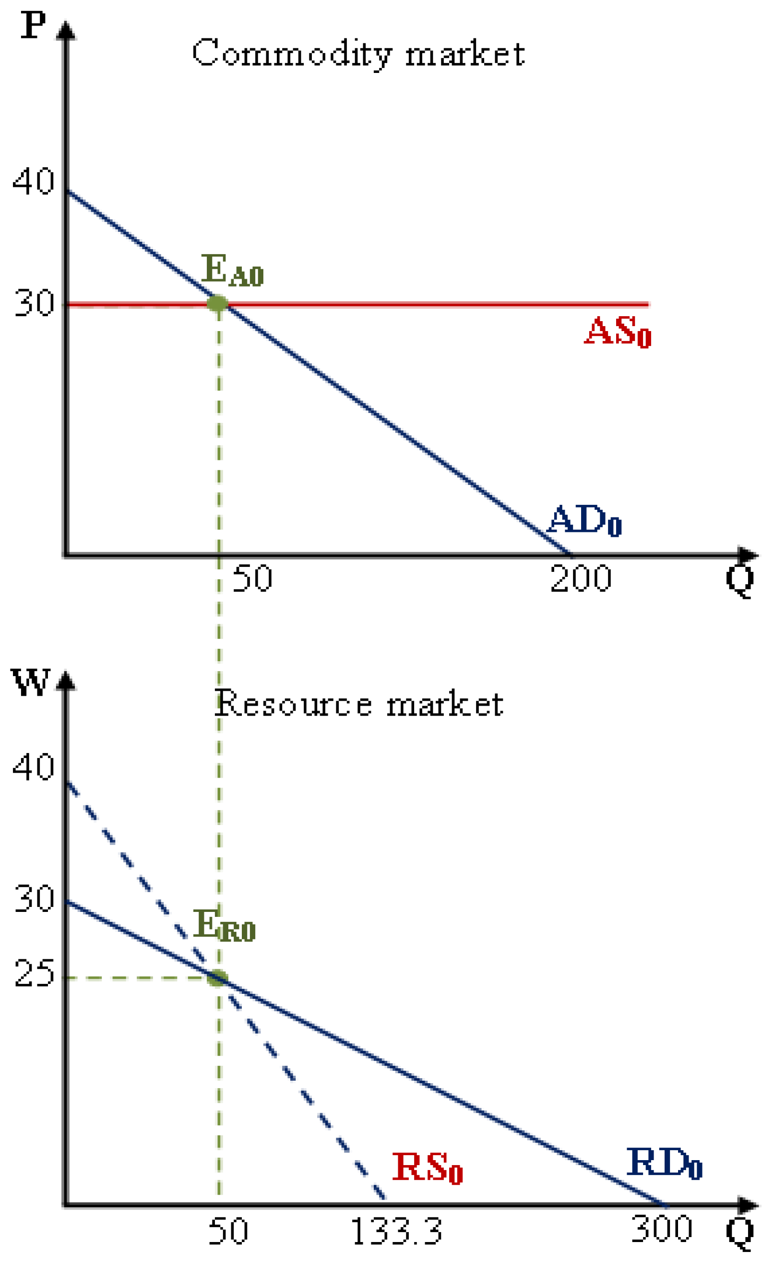
This section illustrates numerical examples of the relationship between the money market and the economy’s structure. The quantity theory of money and the Fisher equation determine the money demand and money supply functions based on the underlying assumptions. Assuming an economy in which the aggregate commodity demand function (pD0) and the aggregate resource demand function (wD0) are given as follows:
The aggregate commodity supply function (pS0) and the aggregate resource supply function (wS0) are determined as follows:
The commodity market equilibrium at the point EA0(p0, QA0) and the resource market equilibrium at the point ER0(w0, QR0) are computed as follows:
Since QA0 = QR0 = Q0, the economy is in the general equilibrium status at the equilibrium quantity (Q0 = 50), as illustrated in Figure 9.
Assume the economy has the current money quantity (M0 = 300), the current nominal interest rates i0 = 7%, and inflation rate f0 = 5%. According to the Fisher equation, the real interest rate (ir) is determined as follows:
From the formula of money quantity, the velocity of money (V) is computed as follows:
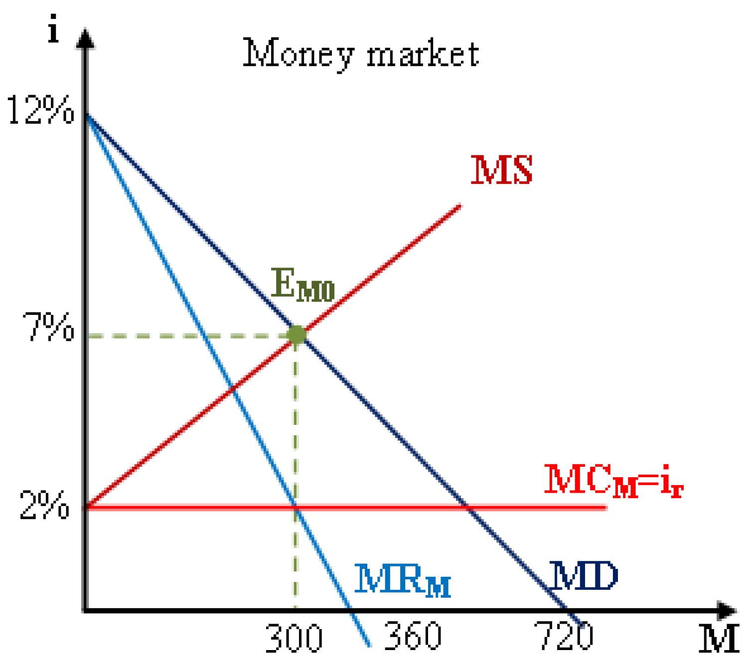
Supposing that the money supply function (iS) and the money demand function (iD) are linear and intersected at the equilibrium point EM0(i0 = 7%, M0 = 300) as follows:
The money supply function (iS) and the money demand function (iD) are rewritten as below.
Figure 10 illustrates the market equilibrium of money for the above example.
The monetary models toward the money market in the general equilibrium framework are considered for three cases: (1) the full-employment equilibrium economy; (2) the steady-state equilibrium economy; and (3) the sticky-price equilibrium economy.
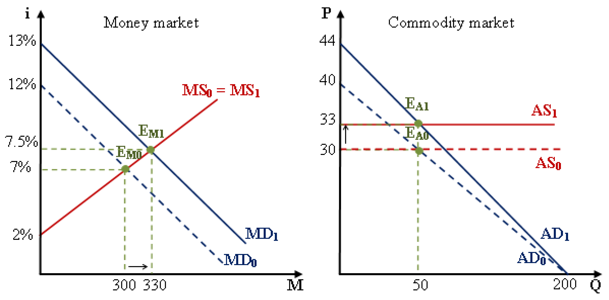
For the full-employment equilibrium economy, the economic growth (nominal national income) is due to an increase in the equilibrium price level p→p1 while the equilibrium quantity (Q) remains constant. Assuming that the equilibrium price level rises at a growth rate of g = 10%, then the aggregate commodity demand function (pD1) and the aggregate resource demand function (wD1) are determined as follows:
The aggregate commodity supply function (pS1) and the aggregate resource supply function (wS1) are determined as follows:
The commodity market equilibrium at the point EA1(p1, QA1) and the resource market equilibrium at the point ER1(w1, QR1) are computed as follows:
Since QA1 = QR1 = 50, the economy is in general equilibrium status with the equilibrium quantity Q1 = 50 and the equilibrium price p1 = 33. According to the quantity theory of money, the money quantity supplied (M1) that assumes a constant velocity of money (V = 5) depends on the quantity Q1 and the price level p1 as follows:
Since the growth rate of inflation reflects the growth rate of the price level (p1 = p0 × (1 + g)), the inflation rate (f1) is determined as follows:
According to the Fisher equation, the nominal interest rate (i1) is computed as follows:
Since the money supply function (iS1) and money demand function (iD1) intersect at the equilibrium point EM1(i1 = 7.5%, M1 = 330), the money supply function (iS1) and the money demand function (iD1) are determined as follows:
When the economy is in the full-employment equilibrium status, the money market equilibrium and the general equilibrium of the economy are illustrated in Figure 11.
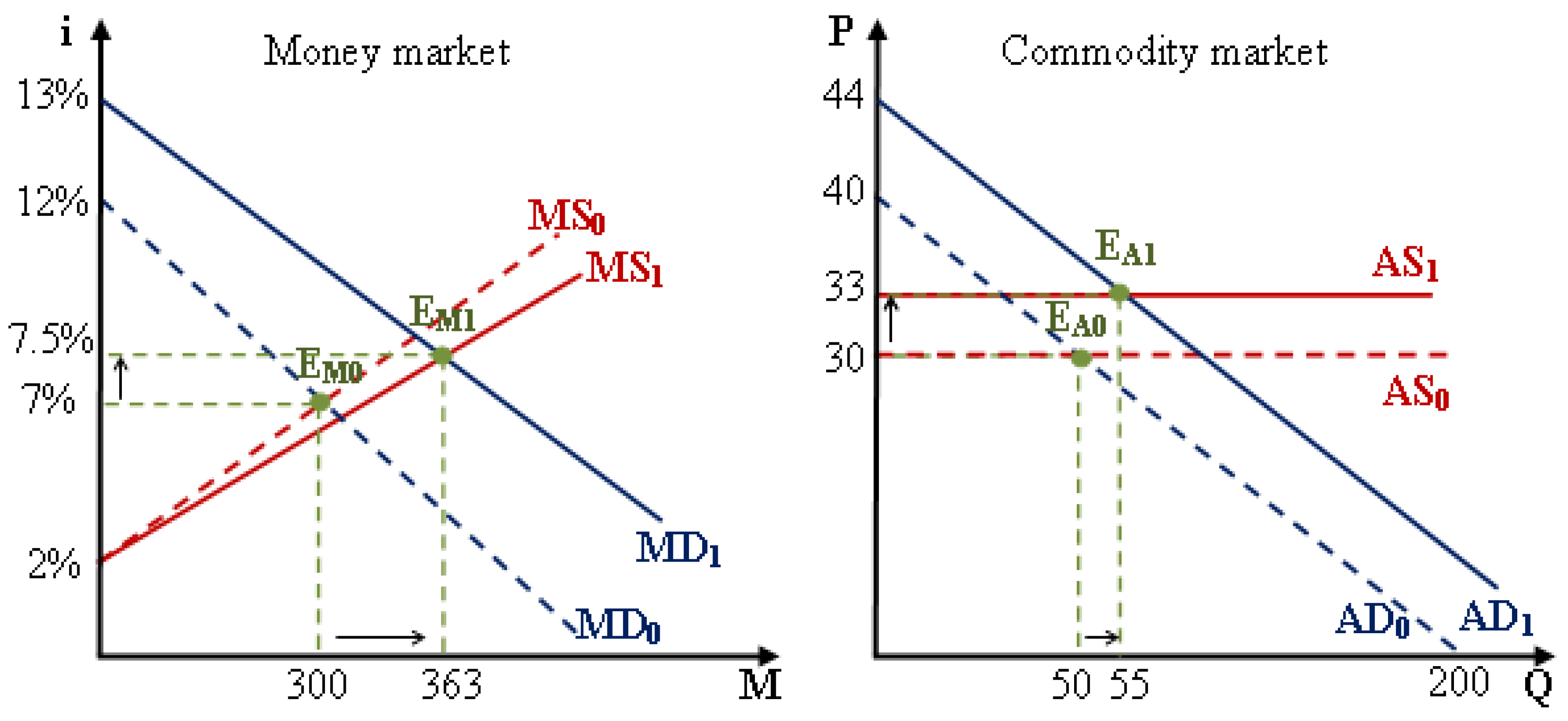
For the steady-state equilibrium economy, the economic growth (nominal national income) is due to an increase in the equilibrium price level p→p1 and an increase in the equilibrium quantity Q→Q1 at the same rate assuming g = 10%. Then, the aggregate commodity demand function (pD1) is determined as follows:
Similarly, the aggregate resource demand function (wD1) is determined as follows:
The aggregate commodity supply function (pS1) and the aggregate resource supply function (wS1) are determined as follows:
The commodity market equilibrium at the point EA1(p1, QA1) and the resource market equilibrium at the point ER1(w1, QR1) are computed as follows:
Since QA1 = QR1 = 55, the economy is in general equilibrium status with the equilibrium quantity Q1 = 55 and the equilibrium price p1 = 33. According to the quantity theory of money, the money quantity supplied (M1) that assumes a constant velocity of money (V = 5) depends on the quantity Q1 and the price level p1 as follows:
Since the growth rate of inflation reflects the growth rate of the price level (p1 = p0 × (1 + g)), the inflation rate (f1) is determined as follows:
According to the Fisher equation, the nominal interest rate (i1) is computed as follows:
Since the money supply function (iS1) and money demand function (iD1) intersect at the equilibrium point EM1(i1 = 7.5%, M1 = 363) as illustrated in Figure 12, thus the money supply function (iS1) and the money demand function (iD1) are determined as follows:
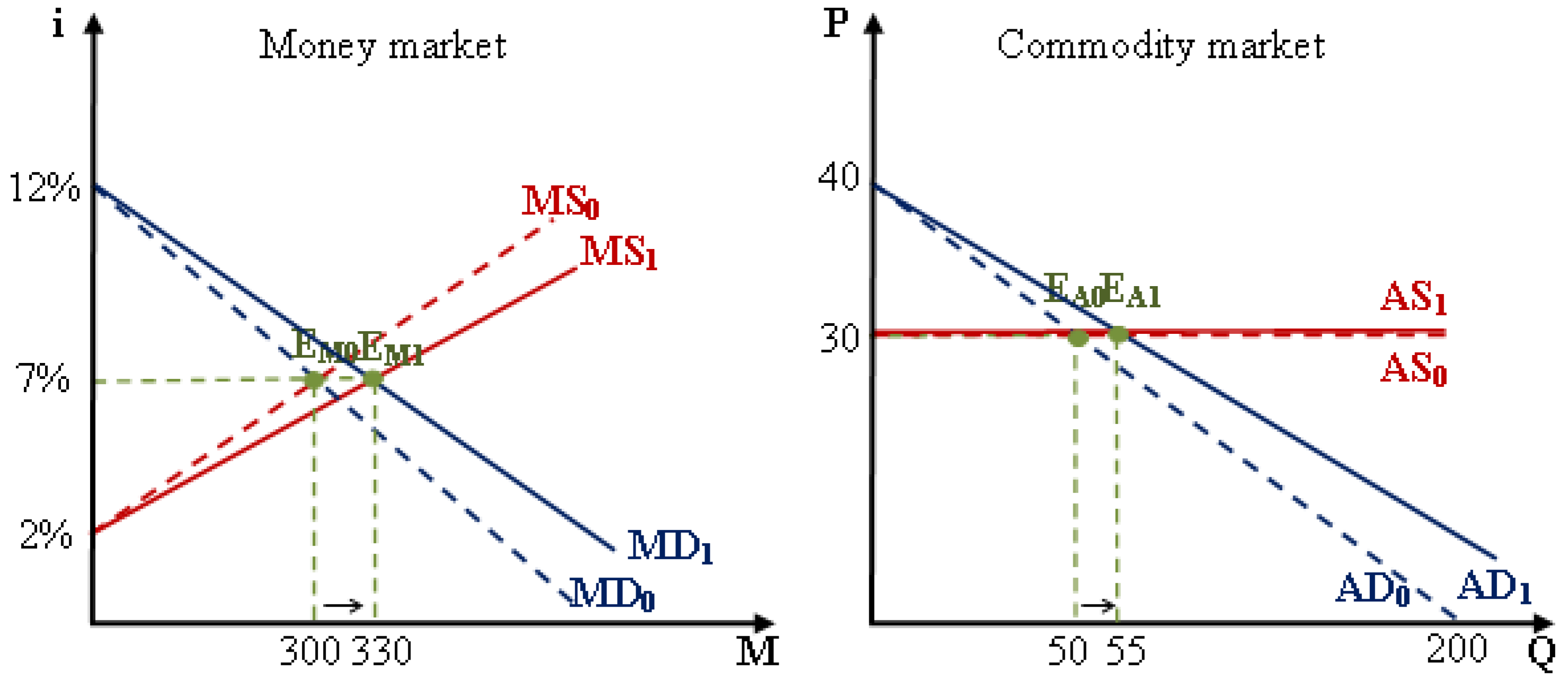
For the sticky-price equilibrium economy, the economic growth (nominal national income) is due to an increase in the equilibrium quantity Q→Q1 at the growth rate assuming g = 10% while the equilibrium price level (p) remains constant. Then, the aggregate commodity demand function (pD1) is determined as follows:
Similarly, the aggregate resource demand function (wD1) is determined as follows:
The aggregate commodity supply function (pS1) and the aggregate resource supply function (wS1) are determined as follows:
The commodity market equilibrium at the point EA1(p1, QA1) and the resource market equilibrium at the point ER1(w1, QR1) are computed as follows:
Since QA1 = QR1 = 55, the economy is in general equilibrium status with the equilibrium quantityQ1 = 55 and the equilibrium price p1 = 30. According to the quantity theory of money, the money quantity supplied (M1) that assumes a constant velocity of money (V = 5) depends on the quantity Q1 and the price level p1 as follows:
Since the equilibrium price remains constant, the growth rate of inflation will be zero g = 0, the inflation rate (f1) is given as follows:
According to the Fisher equation, the nominal interest rate (i1) is computed as follows:
Since the money supply function (iS1) and money demand function (iD1) intersect at the equilibrium point EM1(i1 = 7.5%, M1 = 330), thus the money supply function (iS1) and the money demand function (iD1) are determined as follows:
When the economy is in the sticky-price equilibrium status, the money market equilibrium and the general equilibrium of the economy are illustrated as in Figure 13.
6. Conclusions
The monetary theory is developed upon microfoundations to understand the nature and behavior of the money market. The microfoundations are also an important basis for the explanation of the interrelationship between the commodity market and the resource market in the economy. Keynesian macroeconomic theory and classical general equilibrium theory are approached to define aggregate demand-aggregate supply and explain the general equilibrium mechanism. From these microfoundations together with the quantity theory of money and the Fisher equation, the monetary theory explains money demand—money supply, the relationship between interest rate and inflation through the equilibrium mechanism in the money market.
The monetary models illustrate the transmission mechanism between the money market and the economy under three cases: when the economy is in full-employment equilibrium status, an increase in the money supply increases the nominal price level without affecting actual economic productivity and the real price level. As a result, increasing the money supply raises price and inflation in the same proportions. If the economy is in under-employment equilibrium status, an increase in the money supply will stimulate economic activities, leading to aggregate demand and aggregate supply changes. While inflation reflects the rise in the price level, the increase in money supply relies on the national income (increases in the price and the quantity of the commodity market). When the economy is in sticky-price equilibrium status, an increase in the money supply increases economic activity in the direction of increasing the quantity level without changes in the price level (or unchanged inflation). Since the inflation and interest rates do not change in the money market, the money supply will change in the same proportion as the national income.
The paper contributes to the development of the monetary theory from inheriting the underlying monetary theories with refining the rigorous microfoundations. The monetary models provide the solid foundation for both theoretical and empirical researches on the role of fiscal and monetary policies in economic growth and macroeconomic stability. However, this research still has several limitations, which are also suggestions for further research related to: the nature of the velocity of money, the expansion of money market structure, the uncertainty of monetary demand, and the commodity market structure (aggregate demand-aggregate supply) under economic policies or economic shocks.
Funding
This research is funded by the Ministry of Education and Training (Vietnam) under project number B2020-DNA-12.
Conflicts of Interest
The author declares no conflict of interest regarding the publication of this paper.
References
- Adrian, Tobias, and Hyun Song Shin. 2009. Prices and quantities in the monetary policy transmission mechanism. In Federal Reserve Bank of New York Staff Report No. 396. Amsterdam: Elsevier. [Google Scholar]
- Arestis, Philip, and Malcolm Sawyer. 2008. A critical reconsideration of the foundations of monetary policy in the new consensus macroeconomics framework. Cambridge Journal of Economics 32: 761–79. [Google Scholar] [CrossRef]
- Arrow, Kenneth J., and Gerard Debreu. 1954. Existence of an equilibrium for a competitive economy. Econometrica 22: 265–90. [Google Scholar] [CrossRef]
- Blanchard, Olivier. 2016. Do DSGE models have a future? Revista de Economía Institucional 18: 39–46. [Google Scholar] [CrossRef] [Green Version]
- Carmichael, Jeffrey, and Peter W. Stebbing. 1983. Fisher’s Paradox and the Theory of Interest. The American Economic Review 73: 619–30. [Google Scholar]
- Christiano, Lawrence J., Mathias Trabandt, and Karl Walentin. 2010. DSGE models for monetary policy analysis. In Handbook of Monetary Economics. Amsterdam: Elsevier, Volume 3, pp. 285–367. [Google Scholar]
- Evans, Paul. 1996. Growth and the Neutrality of Money. Empirical Economics 21: 187–202. [Google Scholar] [CrossRef]
- Fama, Eugene F. 1975. Short-Term Interest Rates as Predictors of Inflation. The American Economic Review 65: 269–82. [Google Scholar]
- Fisher, Irving. 1911. The Purchasing Power of Money. New York: Macmillan. [Google Scholar]
- Fisher, Irving. 1930. The Theory of Interest. New York: MacMillan. [Google Scholar]
- Fontana, Giuseppe, and Alfonso Palacio-Vera. 2007. Are long-run price stability and short-run output stabilisation all that monetary policy can aim for? Metroeconomica 58: 269–98. [Google Scholar] [CrossRef] [Green Version]
- Friedman, Milton. 1956. The quantity theory of money: A restatement. Studies in the Quantity Theory of Money 5: 3–31. [Google Scholar]
- Friedman, Milton. 1968. The role of monetary policy. American Economic Review 58: 1–17. [Google Scholar]
- Friedman, Milton, and Anna J. Schwartz. 1965. Money and business cycles. The State of Monetary Economics, 32–78. [Google Scholar] [CrossRef] [Green Version]
- Gaffard, Jean Luc. 2018. Monetary Theory and Policy: The Debate Revisited. LEM Working Paper Series, No. 2018/37; Pisa: Scuola Superiore Sant’Anna, Laboratory of Economics and Management (LEM). [Google Scholar]
- Goodfriend, Marvin, and Robert G. King. 1997. The new neoclassical synthesis and the role of monetary policy. NBER Macroeconomics Annual 12: 231–83. [Google Scholar] [CrossRef]
- Hansen, Alvin Harvey. 1953. A Guide to Keynes. New York: McGraw-Hill Book. [Google Scholar]
- Hicks, John R. 1937. Mr. Keynes and the “classics”; A suggested interpretation. Econometrica: Journal of the Econometric Society 5: 147–59. [Google Scholar] [CrossRef]
- Keynes, John Maynard. 1930. Treatise on Money: Pure Theory of Money Vol. I. London: Macmillan. [Google Scholar]
- Keynes, John Maynard. 1936. The General Theory of Interest, Employment and Money. London: MacMillan. [Google Scholar]
- Lucas, Robert E. 1972. Expectations and the neutrality of money. Journal of Economic Theory 4: 103–24. [Google Scholar] [CrossRef]
- McCallum, Bennett T., and Edward Nelson. 2010. Money and inflation: Some critical issues. Handbook of Monetary Economics 3: 97–153. [Google Scholar]
- Mishkin, Frederic S. 2001. The Transmission Mechanism and The Role of Asset Prices in Monetary Policy. National Bureau of Economic Research. Available online: https://www.nber.org/papers/w8617 (accessed on 29 December 2021).
- Palley, Thomas I. 2007. Macroeconomics and monetary policy: Competing theoretical frameworks. Journal of Post Keynesian Economics 30: 61–78. [Google Scholar] [CrossRef]
- Palley, Thomas I. 2015. Money, fiscal policy, and interest rates: A critique of Modern Monetary Theory. Review of Political Economy 27: 1–23. [Google Scholar] [CrossRef]
- Pigou, Arthur Cecil. 1917. The value of money. The Quarterly Journal of Economics 32: 38–65. [Google Scholar] [CrossRef]
- Romer, David. 2006. Advanced Macroeconomics, 3rd ed. New York: Mcgraw-Hill. [Google Scholar]
- Stiglitz, Joseph E. 2018. Where modern macroeconomics went wrong. Oxford Review of Economic Policy 34: 70–106. [Google Scholar]
- Tavlas, George S. 1981. Keynesian and monetarist theories of the monetary transmission process: Doctrinal aspects. Journal of Monetary Economics 7: 317–37. [Google Scholar] [CrossRef]
- Twinoburyo, Enock Nyorekwa, and Nicholas M. Odhiambo. 2018. Monetary policy and economic growth: A review of international literature. Journal of Central Banking Theory and Practice 7: 123–37. [Google Scholar] [CrossRef] [Green Version]
- Trinh, Truong Hong. 2018. Towards a paradigm on the value. Cogent Economics & Finance 6: 1429094. [Google Scholar]
- Trinh, Truong Hong. 2019. Value Concept and Economic Surplus: A Suggested Reformulation. Theoretical Economics Letters 9: 1920–37. [Google Scholar] [CrossRef] [Green Version]
- Trinh, Truong Hong. 2020. Rational Choice and Market Behavior. In Eurasian Economic Perspectives 14/1. Berlin: Springer, pp. 349–61. [Google Scholar]
- Trinh, Truong Hong. 2021. The Extended Insights into Market Behavior. In Eurasian Business and Economics Perspectives. Berlin: Springer, pp. 225–38. [Google Scholar]
- Walras, Leon. 1874. Elements of Pure Economics. London: George Allen and Unwin, Reprinted 1954. [Google Scholar]
- White, William R. 2013. Is Monetary Policy a Science?: The Interaction of Theory and Practice Over the Last 50 Years. Federal Reserve Bank of Dallas, Globalization and Monetary Policy Institute (Working Paper No. 155). Available online: http://www.dallasfed.org/assets/documents/institute/wpapers/2013/0155.pdf (accessed on 29 December 2021).
- Woodford, Michael. 2005. Firm-Specific Capital and the New-Keynesian Phillips Curve. National Bureau of Economic Research. Available online: https://www.nber.org/papers/w11149 (accessed on 29 December 2021).
Figure 1.
The structure of the simple economy.

Figure 2.
The equilibriums of AD-AS and RD-RS.

Figure 3.
General equilibrium of the economy.

Figure 4.
The equilibrium of the money market.

Figure 5.
Money market and general equilibrium.

Figure 6.
The full-employment equilibrium economy.

Figure 7.
The steady-state equilibrium economy.

Figure 8.
The sticky-price equilibrium economy.

Figure 9.
General equilibrium of the hypothetical economy.

Figure 10.
Money market equilibrium of the hypothetical economy.

Figure 11.
Case of the full-employment equilibrium economy.

Figure 12.
Case of the steady-state equilibrium economy.

Figure 13.
Case of the sticky-price equilibrium economy.

Publisher’s Note: MDPI stays neutral with regard to jurisdictional claims in published maps and institutional affiliations. |
© 2022 by the author. Licensee MDPI, Basel, Switzerland. This article is an open access article distributed under the terms and conditions of the Creative Commons Attribution (CC BY) license (https://creativecommons.org/licenses/by/4.0/).
Share and Cite
MDPI and ACS Style
Trinh, T.H. Towards Money Market in General Equilibrium Framework. Int. J. Financial Stud. 2022, 10, 12. https://0-doi-org.brum.beds.ac.uk/10.3390/ijfs10010012
AMA Style
Trinh TH. Towards Money Market in General Equilibrium Framework. International Journal of Financial Studies. 2022; 10(1):12. https://0-doi-org.brum.beds.ac.uk/10.3390/ijfs10010012
Chicago/Turabian StyleTrinh, Truong Hong. 2022. "Towards Money Market in General Equilibrium Framework" International Journal of Financial Studies 10, no. 1: 12. https://0-doi-org.brum.beds.ac.uk/10.3390/ijfs10010012
Note that from the first issue of 2016, this journal uses article numbers instead of page numbers. See further details here.