South African Banks’ Cross-Border Systemic Risk Exposure: An Application of the GAS Copula Marginal Expected Shortfall

Abstract

Systemic susceptibility highlights the extent to which a banking sector is sensitive to negative shocks. Policymakers and regulators’ objective is to avoid financial crises, and even though they can somewhat control local conditions, internationally transmitted crises are difficult to tackle. This paper analyzes the cross-border systemic risk exposure of South African banks. The marginal expected shortfall is employed with data covering 2002 to 2020. The results show that South African banks are significantly prone to crises emanating beyond the country’s borders. The findings confirm the existence of a significant transfer of risk from other countries to South Africa’s banking sector. Moreover, the amount of foreign capital invested in a bank is found to be a strong predictor of a bank’s international exposure. Knowledge of the linkages that the banking system has with other countries, and how cross-border exposures endanger banks, will form a basis for regulations that ensure a safer financial system.

1. Introduction

The conversation around financial crises and the threat they pose to financial and economic stability needs to be elevated from the country level to a broader global discussion amongst regulators and policymakers. Over the past decade or so, we have witnessed how instabilities emanating from one financial institution propagate to other financial institutions, similarly from financial market to financial market, and ultimately from country to country. Therefore, the focus of these discussions should be on identifying and understanding the system, its risks, and the interlinkages that combine entities, financial markets and countries.

To this end, the magnitude of the cost/loss induced by the financial crisis of 2007–2009 is still to be fully determined. The recent European sovereign debt crisis is one of the latest after-effects of the systemic events of 2007–2009. Funding challenges in the banking sector spilled over to other markets and countries via international transactions and were ultimately transmitted to the sovereign debt market as governments attempted to bail out distressed financial institutions.

The economic literature on systemic risk has focused on different aspects of this phenomenon. Adrian and Brunnermeier (2016), Girardi and Ergün (2013) and Banulescu and Dumitrescu (2015) have all focused on quantifying the marginal contributions of financial institutions to the overall risk of their domestic financial systems. Kallestrup et al. (2016), Alter and Beyer (2014) and Eichengreen et al. (2012) add a component of cross-border trade into systemic risk analysis by investigating the spillovers from a country’s distressed financial system into another country’s financial system. The problem of systemic risk in sovereign debt markets is studied by Reboredo and Ugolini (2015) and is explained as contagion by Gray (2009) and Gómez-Puig and Sosvilla-Rivero (2014).

Most of the literature examines systemic risk from one perspective, that is, how much distressed institutions contribute to the systemic risk of the whole financial system. Nevertheless, the amount of risk that distressed financial systems add to individual institutions is also of great importance in ensuring stability. This rarely studied viewpoint focused on the sensitivity of financial institutions to systemic events is termed systemic risk exposure. Systemic risk exposure, unlike systemic risk contribution, focuses on how much additional risk is faced by individual institutions in the event of market disruption. Thus, this study builds on and contributes to the literature by using a methodology that is flexible enough to cater for time-varying tail dependence. According to Sedunov (2016), institutions that do not initially contribute much to systemic risk, but which are heavily exposed to crises, tend to magnify the distress of the financial system. Against this background, we investigate the cross-border systemic risk exposure of South African banks, and how these banks respond to crises emanating beyond the country’s borders. This will inform regulators and policymakers on the vulnerabilities of South African banks to external markets and assist them to better understand the influences of each institution’s level of systemic risk exposure.

The existing literature in the field of systemic risk and contagion is quite exhaustive. Studies have focused on different aspects, such as the contribution of banks to financial system aggregate risk, the probability of tail events in the banking system, and systemic risk transfer in sovereign debt markets. This study contributes to the existing literature in several ways. First, the analysis focuses on the systemic stress and vulnerability of banks in an attempt to measure how susceptible domestic banks are to foreign shocks. Unlike Foggitt et al. (2019), who treat the financial system as a unity, in this study, we disaggregate and treat banks as individuals, allowing for the banks’ different characteristics to come into play. Moreover, this study differs from others that examine the amount of risk that banks contribute to the aggregate risk of the system, such as that by Manguzvane and Mwamba (2019), who focused entirely on banks’ exposure to crises across borders. Unlike Sedunov (2016), who employs conventional MES, this study uses GAS Copulas in building the MES so as to allow for capturing the dynamic dependence structure between financial assets and markets. The approach offered in this study has several advantages. First, while this study focuses on the banking sector, the techniques presented here can be applied in other sectors, meaning the analysis can be extended to focus on vulnerabilities in other markets, such as sovereign debt. Secondly, the data used in the study are based on banks’ market values, and are readily available, making analysis easy and quick.

The objectives of this paper are two-fold: first, we investigate the systemic risk exposure of South African banks to crises in international financial markets. Second, we determine which international markets have the largest effect on South Africa’s banking sector. These objectives are critical in forecasting how South African banks will perform when there is distress in other countries (mainly the country’s major trading partners), as this will impact the country’s ability to refinance its debts. The reasoning behind studying banks’ systemic risk exposure is that its effects go beyond the banking sector to other markets, such as the sovereign debt, and ultimately affect the welfare of society. Sedunov (2016) claims that a country with a risky banking sector may be more likely to have higher sovereign yields because investors expect greater strain on the government’s finances if the government is forced to bail out those banks. Furthermore, a country that provides financial assistance to systemically distressed financial institutions may increase the riskiness of its sovereign debt. Not only will this affect the sovereign debt, but it will also ultimately affect the real economy, as witnessed during the global financial crisis. Moreover, with the significant influence that South Africa’s biggest banks have throughout the African continent, it is of paramount importance to understand how the banks will respond to international crises, as these will have ripple effects on the already fragile African market.

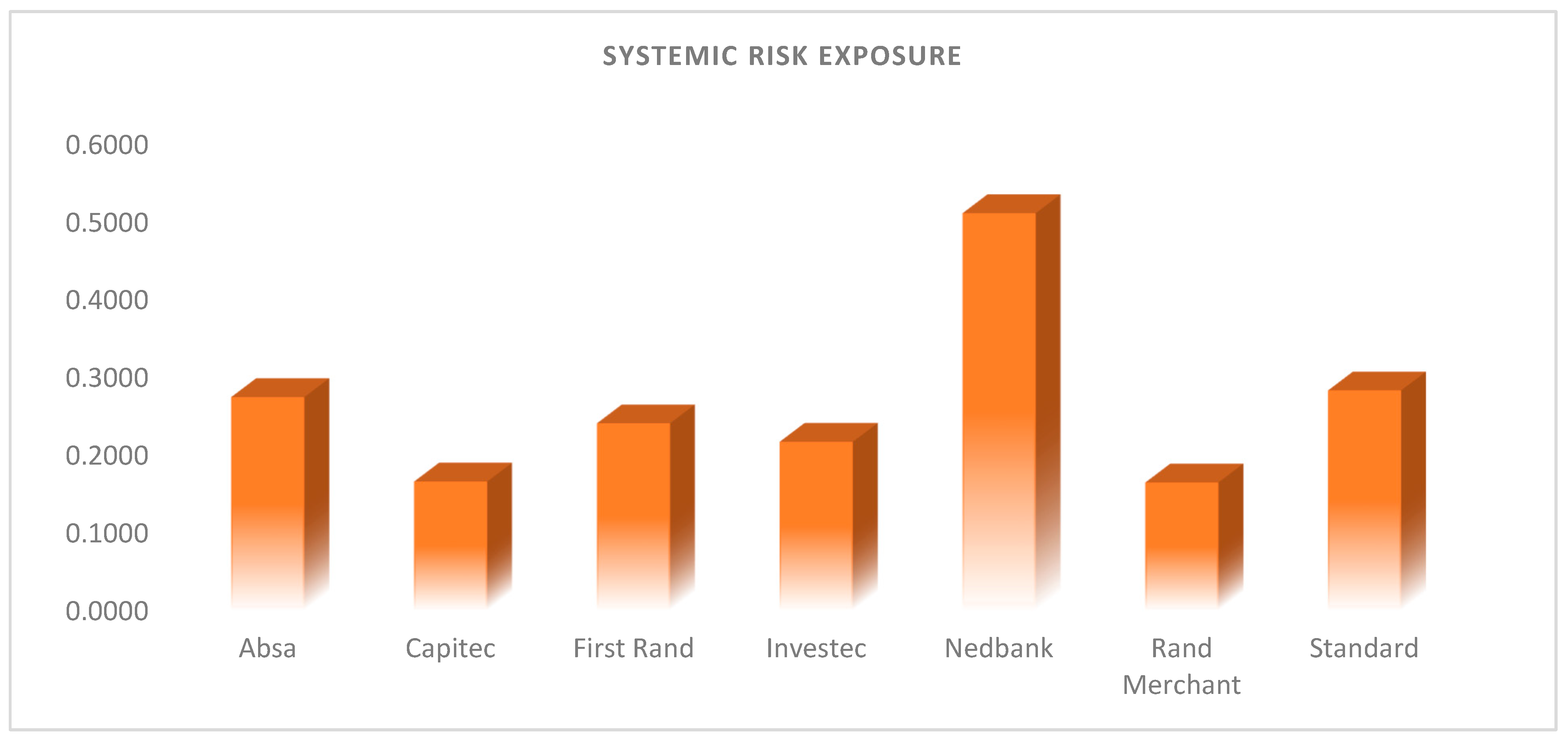
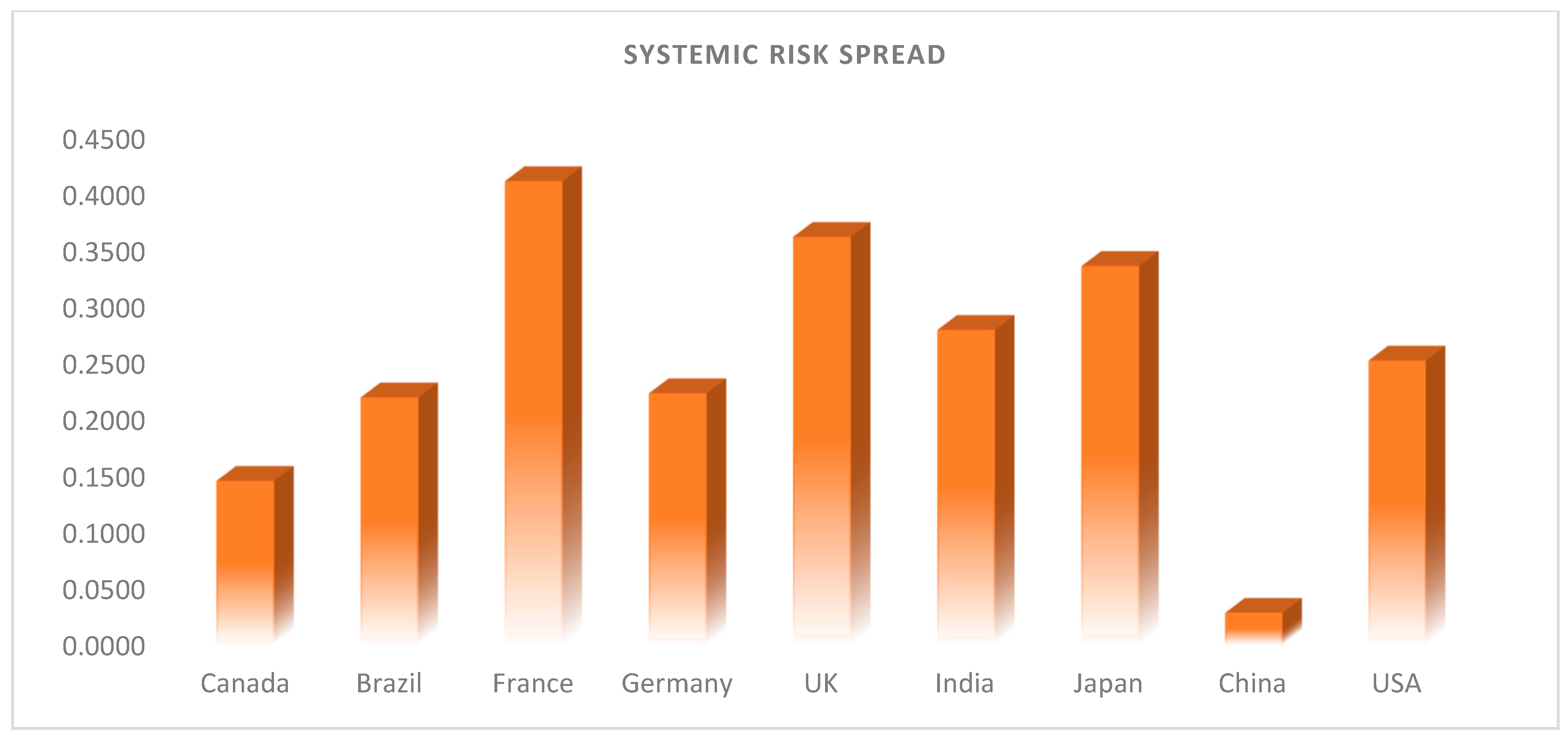
To this end, we measure how distressed international financial markets influence the stability of South Africa’s largest banks. We use available data for seven of the largest banks in South Africa, namely Absa, Capitec, First Rand, Investec, Rand Merchant, Nedbank and Standard Bank, while for international markets, we focus on both developed and emerging economies. The study pays attention to South Africa’s banking sector because, despite being an emerging market, South Africa has a financial services sector that is very well developed. With assets worth over ZAR 6 trillion and contributing more than 10% to GDP, not only does the sector play a vital role in driving the economy forward, but it is also well-placed to be the regional financial center for Africa. The South African banking system’s uniqueness comes in the form that it is relatively large, but heavily concentrated, with around 92 percent of the total assets belonging to only six banks. Moreover, the largest South African banks are heavily active in other African countries, which implies that these banks are not only a threat to South African financial stability, but also pose a systemic threat to a lot of other African countries. South Africa also remains the only Financial Stability Board jurisdiction that does not have an explicit deposit insurance scheme. A deposit insurance scheme is meant to build a comprehensive regulatory system for reducing the social and economic cost of distressed financial institutions.1

The recent rise in pace of globalization requires that the financial sector to be even more integrated with the global financial system. However, integration, along with the reckless chasing of short-term profits, has been proven by the global financial crisis to bring increased stability risk. There is thus an urgent need for regulatory tools that meet international standards and can confirm the build-up of imbalances before they develop into crises. While this study focuses on South Africa only, the findings could be extended to other emerging and developing economies that have similar characteristics to South Africa.

The measure of systemic risk exposure that we use is the marginal expected shortfall (MES). The MES, unlike other systemic risk measures, such as the conditional value at risk (CoVaR), allows us to directly measure the responsiveness of financial institutions to system-wide distress. However, the MES, as proposed by Acharya et al. (2012) and modified by Brownlees and Engle (2012), does not consider the time-variation of the dependence parameter. To cater for this, we follow the approach proposed in Eckernkemper (2018), which uses Copulas to estimate the MES. Copulas offer greater flexibility, as they allow for the separate modeling of marginals and the dependence structure. This separation means that the marginal specification is not restricted by the Copula distribution. As a driving mechanism for time-varying parameters, we use the generalized autoregressive score model (GAS) of Creal et al. (2013). A mixed Copula rather than a one-dimensional Copula is used to model asymmetric dependencies in one framework while also distinguishing between upper and lower tail dependence. The mixed Copula has two components, the first being the Clayton Copula, which captures lower tail dependence, and the second being the rotated Clayton, which takes into account upper tail dependence. Our data, much like most financial time series data, are non-normal; therefore, to capture the skewness and excess kurtosis, we estimate our marginal models via an exponential GARCH using the skewed t distribution.

Using a sample running from March 2002 through to May 2020, we find that, on average, Nedbank and Absa are the banks that would be most vulnerable if an international crisis were to occur. This means that of all the South African banks, Nedbank and ABSA are the most systemically exposed to international distress. The international linkages that the two banks have enjoyed over the years would support these findings. These findings are not by chance as ABSA has been a full subsidiary of UK banking giant Barclays PLC for over 90 percent of our sampling period, making it very vulnerable to any problems that Barclays encounters. The third and fourth most endangered banks in this context are Standard Bank and First Rand, which, together with Nedbank and ABSA, make up the four largest banks in South Africa, which gives rise to the “too big to fail” and the “too interconnected to fail” theories. From a regulatory perspective, this shows which institutions would be seriously endangered if an international crisis ensued. Moreover, knowing the systemic risk exposure of banks will enable regulators and policymakers to identify the determinants of the level of exposure.

The rest of the study is organized as follows: Section 2 presents the empirical literature review related to this study. Section 3 provides an overview of the methodology employed. Section 4 presents a discussion of the results, and Section 5 concludes the study.

2. Literature Review

The literature on systemic risk has expanded rapidly since the onset of the global financial crisis, mainly highlighting the importance of investigating this global phenomenon. Interestingly, little empirical evidence has been provided on the transfer of systemic risk across borders or the susceptibility of banks in one country to crises emanating from across borders. This paper, however, relates to multiple strands of literature. The first stream of literature that relates to the current study focuses on quantifying the amount of risk that one financial institution poses to its domestic financial system when it is under stress. For example, Laeven et al. (2016) employed the CoVaR and MES to measure the systemic risk contribution of financial institutions with a market capitalization of more than USD 10 billion in over 30 countries. Their findings are substantiated by Buch et al. (2019), who show that the systemic risk contribution is closely related to both the relative and the absolute size of a bank. Similarly, Pham et al. (2021) examined the systemic risk contribution of Asian banks through the application of four techniques, namely, the CoVaR, SRISK, component expected shortfall, and the MES. The four methodologies are found to be consistent in quantifying the amount of risk each bank adds to the aggregate risk of the system.

Several other studies have indulged in this stream of research. Manguzvane and Mwamba (2019) applied the CoVaR technique to model systemic risk in the South African banking sector, whereas Karimalis and Nomikos (2018) proposed a Copula-based CoVaR to examine the common market factors that trigger systemic risk periods. Billio et al. (2012) employed granger causality tests and principal component analysis to examine systemic risk in the US and found a large number of interconnections that pose a real threat to financial markets as a whole.

An interesting strand in the literature takes an opposite view from the first strand. This group examines how financial institutions are affected when the whole financial system is in distress. This strand looks at the systemic risk exposure of institutions. Acharya et al. (2012) developed the marginal expected shortfall, which measures how the equity value of a given financial institution will drop when the financial system enters distress. Sedunov (2016) used several measures to investigate the amount of systemic risk exposure that US banks face. This study is based on the premise that regulators do not have relevant knowledge on the exposure of financial institutions, hence rendering them ineffective in managing institutions during crisis. Thus, their study focuses on assessing which institutions will be seriously affected by a financial crisis by employing the MES and exposure CoVaR. First, they find that the exposure CoVaR captures systemic risk exposure much more effectively compared to the MES. Secondly, their results show that the exposure of institutions to the risk posed by the markets was very high just before and during the global financial crisis. Brownlees and Engle (2012) derived similar results in a study measuring the expected capital shortfall of a firm following a severe market decline. Their results were obtained by employing the SRISK measure, which is an extension of the MES and has proven to be very useful in outlining the events that took place during the subprime mortgage crisis.

A third strand in the literature concentrating on systemic risk focuses on cross-border linkages. Several studies have taken this route; among them, Drakos and Kouretas (2015) examined the effect of foreign banks on the stability of the US financial system. Their analysis, based on data collected from 2000 through 2012, concludes that non-US banks contribute significantly to the disruption of the provision of financial services and financial instability in the US. However, this contribution is relatively low compared to that of domestic banks. Dungey and Gajurel (2015) employed GARCH models to investigate whether banks’ increased international exposure destabilizes the domestic financial sector. The study covered 45 countries, and the results show that crisis shocks transmitted from a foreign jurisdiction via idiosyncratic contagion increase the likelihood of a systemic crisis.

Tonzer (2015) took a similar approach by analyzing whether international linkages in interbank markets affect the stability of interconnected banking systems. They applied a relatively new technique in the field of financial economics in the form of spatial econometrics using bilateral cross-border banking exposure data collected from the Bank of International Settlements. Evidence from this study suggests that foreign exposures in the banking sector are a significant contributor to overall banking risk across countries. A more recent example is Foggitt et al. (2019), who studied the transfer of risk from the US to South Africa. Instead of only using traditional MES, they combined it with the DCC GARCH model, and the results show a strong spillover of systemic risk from the US to South Africa.

Xu et al. (2021) dealt with the problem of risk transmission between different economic sectors. Employing a tail-driven network to study dependence, the authors found that the banking sector is the principal risk-spreader in the Chinese economy. Similarly, Zhu et al. (2021) showed how sector-induced contagion effects propagate during economic and financial crises. Their findings, obtained using time-varying Copulas, reveal the presence of significant systemic risk spillovers between the energy and agriculture sectors.

Another strand in the literature that is closely related to our study focuses on the transmission of shocks between countries’ sovereign debt markets. This pays attention to how changes in one country’s sovereign debt yields are influenced by another’s debt yields. Beirne and Fratzscher (2013) concentrated on analyzing whether there was contagion during the European sovereign debt crisis. Using data collected from 31 countries, including some emerging market economies, their analysis concluded that there was significant contagion between 2010 and 2012. Spreads of between 100 and 200 basis point increases in the sovereign yields of European countries, such as Greece, Italy, Portugal and Spain, have been attributed to international risk spillovers. Similarly, Brutti and Sauré (2015) analyzed the role played by financial interlinkages in the transmission of risk between European states during the European sovereign debt crisis. The empirical part of this study is based on a vector autoregressive model, augmented to cater for time-varying shock transmission. Lucas et al. (2014) applied GAS models in assessing the likelihood of joint and conditional sovereign debt defaults in Europe. They found strong evidence of time-varying distress dependence and spillover effects in sovereign default risk. These findings are supported by Reboredo and Ugolini (2015), who applied Copula CoVaR, and found that before the debt crisis, sovereign debt markets were all coupled, and systemic risk was similar for most countries. Borri (2018) investigated the susceptibility of emerging countries to systemic risk for local currency-denominated government debt. A quantile regression-based CoVaR was employed, and their findings reveal that emerging countries’ vulnerabilities increase with the share of local currency-denominated debt held by foreign investors.

3. Methodology

3.1. Marginal Expected Shortfall

Let $X_t={(X_{i,t}, X_{m,t})}^T$ represent the vector of equity market returns for two assets, where $X_{i,t}$ is the return for institution i and $X_{m,t}$ is the return of the entire market. The information set available at time $t-1$ is denoted by ${\mathsf{\Omega }}_{t-1}$ and $\left(X_{i,t-1}, X_{m,t-1}\right)\subseteq {\mathsf{\Omega }}_{t-1}$, and $\mathrm{F}(.;{\mathsf{\Omega }}_{t-1})$ is the joint cumulative distribution function (cdf) of $X_t$ given ${\mathsf{\Omega }}_{t-1}$, such that $\mathrm{F}(x_t;{\mathsf{\Omega }}_{t-1})\equiv P\left(X_{i,t}\le x_{i,t},X_{m,t}\le x_{m,t}{|\mathsf{\Omega }}_{t-1}\right)$ for any $x={(x_{i,t},x_{i,t})}^T\in R^2$. We assume that the cdf of $X_t$ is continuous.

The expected shortfall (ES) of the market, which is used to measure the risk of the market, is given by:

$$E{S}_{m,t}=E_{t-1}(X_{m,t}|X_{m,t}\le Z_t)$$

(1)

where $Z_t$ is a predefined threshold, such as the Value at Risk.

Given that the return of the market is a linear combination of the returns of the individual institutions and is given by

$$X_{m,t}={{\displaystyle \sum }}_{i=1}^n{w}_i{X}_{i,t}$$

(2)

where $w_i$ is institution i’s market share, we can decompose Equation (1) as follows

$$E{S}_{m,t}=E_{t-1}\left({{\displaystyle \sum }}_{i=1}^n{w}_i{X}_{i,t}|X_{m,t}\le Z_t\right)={{\displaystyle \sum }}_{i=1}^n{w}_{i,t}{E}_{t-1}(X_{i,t}|X_{m,t}\le Z_t)$$

(3)

According to Acharya et al. (2012), the marginal expected shortfall (MES) corresponds to the derivative of the market’s expected shortfall with respect to institution i’s market share.

$$ME{S}_{i,t}=\frac{\partial E{S}_{m,t}}{\partial w_i}=E_{t-1}(X_{i,t}|X_{m,t}\le Z_t)$$

(4)

The MES measures the expected return of institution i given that the return of the market has crossed the threshold $Z_t$.

Brownlees and Engle (2012) modified the MES measure by including volatility and correlation in a bivariate model for the return of institution i and the market. The return for institution i and market can be represented as in Brownlees and Engle (2012), as follows:

$$\begin{gathered} X_{i,t}={\mu }_{i,t}+{\sigma }_{i,t}⨀{\epsilon }_{i,t} \\ {X}_{m,t}={\mu }_{m,t}+{\sigma }_{i,t}{\rho }_{i,t}{\epsilon }_{i,t}+{\sigma }_{m,t}+\sqrt{1}-{\rho }_i^2{\eta }_{m,t} \end{gathered}$$

(5)

where ${\epsilon }_{i,t}$ and ${\eta }_{m,t}$ are independent error terms, ${\sigma }_{i,t}$ and ${\sigma }_{m,t}$ are the conditional standard deviations for the institution and market, respectively. The conditional volatilities are estimated using an EGARCH model and the conditional correlation is modeled using a Diagonal Conditional Correlation GARCH. The new definition of MES according to Brownlees and Engle (2012) becomes

$$MES=E_{t-1}({\sigma }_{i,t}{\rho }_{i,t}{\epsilon }_{i,t}+{\sigma }_{m,t}+\sqrt{1}-{\rho }_i^2{\eta }_{m,t}|{\sigma }_{m,t}{\epsilon }_{m,t}\le Z_t)$$

(6)

Equation (6) can be further simplified as follows

$$MES={\sigma }_{i,t}{\rho }_{i,t}{E}_{t-1}({\epsilon }_{m,t}|{\epsilon }_{m,t}\le k_t+{\sigma }_{i,t}+\sqrt{1}-{\rho }_i^2)$$

(7)

where $k_t=\frac{C_t}{{\sigma }_{m,t}}$.

3.2. GAS Copula MES

3.2.1. Copulas

An n-dimensional Copula is a function C from ${\left[0,1\right]}^n\to \left[0,1\right]$ with the following properties:

(1)

$C\left(u_1,\dots ,u_n\right)$ is decreasing in each component $u_i$ $\in \left[0,1\right] i=1,\dots ,n$

(2)

$C\left(1,\dots 1,u_i,1\dots 1\right)=u_i$ for $u_i$ $\in \left[0,1\right] i=1,\dots ,n$

Property (1) implies that the Copula is a multivariate cumulative density function. Property (2) suggests that the Copula has uniform margins. It is apparent that the Copula is nothing but a multivariate distribution. However, the Copula has its own power when dealing with multivariate distributions. This power is derived from Sklar’s theorem. For any random variable $X_1,\dots , X_n$ with joint CDF $F\left(x_1,\dots , x_n\right)=P(X_1\le x_1,\dots , X_n\le x_n$ and marginal CDFs $F_i\left(x_i\right)=P\left(X_i\le x_i\right)$ for $=1\dots n$, there exists a Copula such that

$$F\left(x_1,\dots , x_n\right)=C\left(F_1\left(x_1\right),\dots F_n\left(x_n\right)\right)=C\left(u_1,\dots ,u_n\right),x_1,\dots , x_n \in ℝ$$

(8)

If $F_i$ are continuous for $i=1,\dots ,n$, then C is unique. If C is a Copula and $F_1,\dots ,F_n$ are univariate distribution functions, the function F defined above is a multivariate distribution function with margins $F_1,\dots ,F_n$.

3.2.2. Classes of Copula

• Gaussian Copula

Given $={(u_1,u_2)}^T\in {[0,1]}^2$, the Gaussian Copula can be formally written as follows

$$C_G\left(u_1,u_2,\rho \right)={\mathsf{\Phi }}_{k,\mathsf{\Sigma }}({\mathsf{\Phi }}^{-1}\left(u_1\right){\mathsf{\Phi }}^{-1}\left(u_2)\right)$$

(9)

where $\mathsf{\Sigma }$ is 2*2 correlation matrix, $\mathsf{\Phi }()$ is the standard normal distribution function and ${\mathsf{\Phi }}^{-1}()$ is the inverse of the $\mathsf{\Phi }()$. This Copula does not cater for tail dependence.

• Archimedean Copulas

Archimedean Copulas are developed by specifying a generator function. Given $\phi$, a generator function with ${(\phi )}^{-1}$ being completely monotonic, then a bivariate Archimedean Copula can be specified as follows:

$$C\left(u_1,u_2,\right)={\phi }^{-1}\left(\phi \left(u_1\right)+\phi \left(u_2\right)\right)$$

(10)

Different forms of Archimedean Copulas exist as results of diverse generator functions and the dependence they consider.

• Clayton Copula

The Clayton Copula has the following generator function $\phi ={(-\log \left(t\right))}^{\theta }$ where $\theta \in \left[1,+\infty \right]$, and $\theta$ is the Copula parameter. The Clayton Copula only caters for lower tail dependence, and in the bivariate case it is given by the following formula:

$$C_C\left(u_1,u_2,\theta \right)={(u_1^{-\theta }+u_2^{-\theta }-1)}^{\raisebox{1ex}{$1$}\!\left/ \!\raisebox{-1ex}{$\theta $}\right.}$$

(11)

The coefficient for lower tail dependence is given by ${\lambda }_L=2^{-\raisebox{1ex}{$1$}\!\left/ \!\raisebox{-1ex}{$\theta $}\right.}$

• Rotated Clayton

The rotated Clayton Copula accounts for upper tail dependence, and its bivariate Copula function is given as follows:

$$C_{RC}\left(u_1,u_2,\theta \right)=u_1+u_2+C_C\left(1-u_1,1-u_2;\theta \right)$$

(12)

• Mixture Copulas

In addition to the Copulas presented above, one can consider a mixture Copula, which is simply the convex combination between different Copula functions. This makes it possible to obtain any dependence structure desired. A mixture of K Copulas is defined as

$$C_M\left(u_1,u_2,\theta \right)={{\displaystyle \sum }}_{i=1}^2{w}_i{C}_i\left(u_1,u_2,{\theta }_i\right)$$

(13)

where ${{\displaystyle \sum }}_{i=1}^K{w}_i=1$, and $w_i$ is the weight for the ith Copula, which lies between 0 and 1.

The conditional expectation in Equation (4) can be expressed as a Copula function as follows:

$$E_{t-1}({\epsilon }_{m,t}|{\epsilon }_{m,t}\le k_t)=\frac{1}{\alpha }{{\displaystyle \int }}_0^1{F}^{-1}\left(u_i\right)\frac{\partial C_t\left(u_i,{\theta }_t\right)}{\partial u_i}d{u}_i$$

(14)

where $\alpha =F_{m\left(k\right)}$. Equation (16) presents the foundation for the GAS Copula MES.

The GAS Copula MES is an extension of the model developed by Brownlees and Engle (2012). The marginal distributions are modeled with an EGARCH model, and the dependence structure is modeled using a Copula function. Setting $X_{m,t}={\sigma }_{m,t}{\epsilon }_{m,t}$ and $X_{i,t}={\sigma }_{i,t}{\epsilon }_{i,t}$ and inserting them into Equation (4), we obtain

$$ME{S}_{i,t}={\sigma }_{i,t}{E}_{t-1}({\epsilon }_{i,t}|{\epsilon }_{m,t}\le k)$$

(15)

Combining Equations (16) and (17), we obtain the GAS Copula MES:

$$\mathrm{GAS}\mathrm{Copula}\mathrm{MES}=\frac{{\sigma }_{i,t}}{\alpha }{{\displaystyle \int }}_0^1{F}^{-1}\left(u_i\right)\frac{\partial C_t\left(u_i,{\theta }_t\right)}{\partial u_i}d{u}_i$$

(16)

where $F^{-1}$ is the quantile function and $C_t$ is the Copula function.

Equation (18) represents a GAS Copula MES for a one-dimensional Copula; however, it can be rewritten for a 2-dimensional mixture Copula as follows:

$$\mathrm{GCMES}=\tilde{w}\frac{{\sigma }_{i,t}}{\alpha }{{\displaystyle \int }}_0^1{F}^{-1}\left(u_i\right)\frac{\partial C_{1,t}\left(u_i,{\theta }_{1,t}\right)}{\partial u_i}d{u}_i+\left(1-\tilde{w}\right)\frac{{\sigma }_{i,t}}{\alpha }{{\displaystyle \int }}_0^1{F}^{-1}\left(u_i\right)\frac{\partial C_{2,t}\left(u_i,{\theta }_{2,t}\right)}{\partial u_i}d{u}_i$$

(17)

where $\tilde{w}$ represents the Copula weight. In this study, we chose to use a mixture containing the Clayton Copula and the rotated Clayton Copula to create a flexible dependence structure. The Clayton Copula caters for lower tail dependence and the survival Clayton considers upper tail dependence. A mixture of these two allows us to model both upper and lower tails at the same time.

3.3. Estimation Procedure

First, the returns of each institution and the market are assumed to follow the pattern AR (1)—EGARCH (1,1). Second, the dependence structure and the Copula parameters ${\theta }_{1,t}$ and ${\theta }_{2,t}$ are estimated via a Copula. The Copula we employ in this study uses the Generalized Autoregressive Score (GAS) dynamics of Creal et al. (2013) as a driving mechanism for the time-varying Copula’s parameters. Formally, the modified measure is based on a time-varying Copula whose dependence parameter is driven by the score of the Copula function. The GAS-backed MES measure has several advantages. Firstly, by using the full density structure, it goes beyond the first and second moments; hence, it captures all the vital information. Additionally, according to Creal et al. (2013), “using the score to update time varying parameters represents the steepest ascent direction for improving the model’s fit given the current position of the parameter”.

The return for the institution and the market model is given by

$$\begin{gathered} X_t={(X_{i,t},X_{m,t})}^T \\ {X}_t={\alpha }_0+{\alpha }_1{X}_{t-1}+{\epsilon }_t \end{gathered}$$

(18)

$${\epsilon }_t={\sigma }_t{Z}_t$$

$$\ln \left({\sigma }_t^2\right)={\beta }_0+\frac{{\beta }_1{\epsilon }_{t-1}+\gamma \left|{\epsilon }_{t-1}\right|}{{\sigma }_t^2}+{\beta }_2\ln \left({\sigma }_{t-1}^2\right)$$

The joint CDF for ${\epsilon }_{m,t}$ and ${\epsilon }_{i,t}$ is given by

$$F_t\left({\epsilon }_m,{\epsilon }_i\right)=\tilde{w}{C}_{1,t}\left[u_i;{\theta }_{1,t}\left(f_{1,t}\right)\right]+\left(1-\tilde{w}\right)C_{2,t}\left[u_i;{\theta }_{2,t}\left(f_{2,t}\right)\right]$$

(19)

where ${\theta }_{1,t}\left(f_{1,t}\right)$, the time-varying parameter, is modeled using GAS dynamics as follows

$$f_{t+1}=\omega +A{s}_t+B{f}_t$$

(20)

$$s_t=S_t{\nabla }_t$$

$${\nabla }_t=\frac{\partial log{C}_t(u_{i,t};{\theta }_t\left(f_t\right),\tilde{w}|{ℱ}_{t-1})}{\partial {\mathrm{f}}_t}$$

where $log{C}_t=log\left[\tilde{w}{C}_{1,t}\left[u_i;{\theta }_{1,t}\left(f_{1,t}\right)\right]+\left(1-\tilde{w}\right)C_{2,t}\left[u_i;{\theta }_{2,t}\left(f_{2,t}\right)\right]\right]$, where ${ℱ}_{t-1}$ represents the information set available at t.

The GAS Copula MES is estimated in two steps. The first involves estimating the marginal models and the second involves estimating the Copula parameters. The score of the density is given by

$$\begin{array}{l}{\nabla }_t\\ =(\tilde{w}\partial C_{1,t}\left[u_i;{\theta }_{1,t}\left(f_{1,t}\right)\right]·\frac{1}{\tilde{w}{C}_{1,t}\left[u_i;{\theta }_{1,t}\left(f_{1,t}\right)\right]+\left(1-\tilde{w}\right)C_{2,t}\left[u_i;{\theta }_{2,t}\left(f_{2,t}\right)\right]}\\ +\tilde{w}\partial C_{2,t}\left[u_i;{\theta }_{2,t}\left(f_{2,t}\right)\right]·\frac{1}{\tilde{w}{C}_{1,t}\left[u_i;{\theta }_{1,t}\left(f_{1,t}\right)\right]+\left(1-\tilde{w}\right)C_{2,t}\left[u_i;{\theta }_{2,t}\left(f_{2,t}\right)\right]})\end{array}$$

(21)

The score of the density is derived analytically. There are different forms that the scaling function can take. The more commonly used scaling function in its general form is given by $S_t={[I\left(X_t|f_t,\omega ,A,B\right)]}^{\zeta }$, where $I\left(X_t|f_t,\omega ,A,B\right)$ is the Fisher information matrix and can be rewritten as follows:

$$I\left(X_t|f_t,\omega ,A, B\right)=-E_{t-1}\left[\frac{{\partial }^{2}lnP(X_t|f_t,\omega ,A,B)}{\partial f_t\partial f_t^T}\right]=E_{t-1}\left[{\nabla }_t{\nabla }_t^T\right]$$

(22)

where $E_{t-1}$. The expectation denotes expectation taken with respect to the conditional distribution of $X_t$. By setting $\zeta =-1$, we obtain the inverse Fisher information matrix, which is the most popular. However, this scaling has been proven to be inconvenient for mixed Copulas; hence, in this study, we follow Eckernkemper (2018) by using $S_t=I$.

4. Empirical Application

4.1. Data

For the main analysis, weekly equity returns data, covering the period March 2002 to May 2020 for seven South African banks and nine financial markets, are collected from Thomson Reuters database. The banks used in this study are Absa, Capitec, First Rand, Rand Merchant, Investec, Nedbank and Standard Bank. The international markets are drawn from both the developed world and emerging markets, and they cover the USA (S&P500), the UK (FTSE100), Germany (DAX), France (CAC 40), Japan (NIKKEI 100), Canada (TSX Composite Index), China (Shanghai Composite Index), India (NIFTY 50) and Brazil (iBovespa). The banks in this study are selected on the basis of the availability of data, and the fact that they are the only commercial banks regarded as domestic commercial banks by regulators in South Africa. The sample period starts in 2002 so as to ensure that all the selected banks have data that run throughout the entire sample period.

4.2. Descriptive Statistics

Table 1. Descriptive Statistics.

	Mean	Std Dev	Kurtosis	Skewness	Minimum	Maximum
Brazil	0.0833	1.5420	3.8977	−0.5930	−9.1960	8.1245
China	0.0301	1.5242	3.6159	−0.6870	−10.1817	4.9186
France	0.0021	1.3042	4.3558	−0.4314	−6.5644	7.3708
Germany	0.0385	1.3714	3.3858	−0.6294	−6.8881	6.5406
India	0.1017	1.4485	6.4521	−1.0779	−10.6405	6.8608
United States	0.0455	1.0464	5.7489	−0.5524	−5.4866	6.6046
United Kingdom	0.0075	1.0499	5.6675	−0.3648	−5.2902	7.2479
Canada	0.0314	0.9493	9.7038	−1.4018	−7.7611	4.3535
Japan	0.0333	1.3793	5.5096	−0.7552	−8.7471	7.7673
Capitec	0.2913	2.0699	7.7490	0.5467	−12.296	17.609
Nedbank	−0.0097	1.8723	17.4731	−1.6156	−20.707	10.015
Absa	0.0462	1.7459	5.9528	−0.2576	−13.305	10.279
First Rand	0.0836	1.7454	2.0279	−0.0800	−8.5409	8.6464
Standard	0.0538	1.6770	2.6262	−0.1926	−8.7409	7.2206
Rand Merchant	0.0878	1.7111	2.3106	−0.1989	−9.9037	7.4659
Investec	0.0337	1.9372	3.2985	−0.4896	−11.191	8.4193

reports the descriptive statistics, which are the mean, standard deviation, maximum, minimum, kurtosis and skewness, for the South African banks and the international financial markets from 2002 through May 2020. Amongst the South African banks, Capitec has the highest mean (0.2913) and the largest standard deviation of 2.0699. This implies that, on average, Capitec has the highest return, while at the same time being the riskiest institution to invest in. Nedbank has the lowest average return, whereas Standard is the least risky, as measured by the volatility of its returns. The sample skewness coefficients, which are mostly negative, suggest longer left tails, while the sample kurtosis coefficients for half of the banks are greater than three, indicating tails that are slightly fatter than those of a normal distribution. Looking at the international markets, China proves to be the most volatile, as measured by the standard deviation. This is no surprise, as we expected one of the emerging markets to be the most volatile. Canada, with a standard deviation of 0.9493, is the least volatile. Just as with South African banks, the data for the international financial markets exhibit characteristics that are common in financial time series data, such as longer left tails that are fatter than those of the normal distribution.

4.3. Marginal Model Results

The marginal model used in this study is the AR(1)-EGARCH(1,1). This model is selected as it is able to capture the leverage effect and avoids the possibility of having negative variance. The results presented in

Table 2. Marginal Model Results.

	Standard	Rand Merchant	Nedbank	First Rand	Capitec	Absa	Investec
mu	0.0576	0.0942 *	0.0215	0.0886 *	0.2872 ***	0.0536 *	0.0265
	(0.0403)	(0.0459)	(0.0473)	(0.0473)	(0.0613)	(0.0285)	(0.0528)
ar1	−0.1523 ***	−0.1196 ***	−0.0775 **	−0.1066 ***	0.0146	−0.1131 ***	−0.0339
	(0.0327)	(0.0294)	(0.0338)	(0.0338)	(0.0324)	(0.0272)	(0.0337)
omega	0.0367 *	0.0531 **	0.0293 ***	0.0542 **	0.0748	0.0317	0.0490
	(0.0202)	(0.0212)	(0.0067)	(0.0219)	(0.0713)	(0.0611)	(0.0362)
alpha1	−0.0939 ***	−0.1453 ***	−0.0848 ***	−0.1480 ***	−0.0633 *	−0.0645 ***	−0.0786 ***
	(0.0260)	(0.0343)	(0.0208)	(0.0329)	(0.0403)	(0.0153)	(0.0282)
beta1	0.9568 ***	0.9441 ***	0.9710 ***	0.9447 ***	0.9443 ***	0.9665 ***	0.9591 ***
	(0.0222)	(0.0201)	(0.0033)	(0.0200)	(0.0536)	(0.0633)	(0.0298)
gamma1	0.2000 ***	0.1130 ***	0.1295 ***	0.1121 ***	0.2343 ***	0.1732 ***	0.1895 ***
	(0.0513)	(0.0371)	(0.0493)	(0.0357)	(0.0735)	(0.0374)	(0.0548)
skew	1.0399 ***	1.0162 ***	0.9218 ***	0.9747 ***	1.0739 ***	1.0181 ***	0.8779 ***
	(0.0507)	(0.0470)	(0.0440)	(0.0459)	(0.0446)	(0.0458)	(0.0397)
shape	11.6318 ***	11.0706 ***	9.2530 ***	14.2276 **	4.3135 ***	7.8351 ***	9.1857 ***
	(3.6899)	(3.5385)	(2.4964)	(5.6548)	(0.6793)	(1.6203)	(2.6448)
Loglikelihood	−1749	−1790	−1804	−1808	−1917	−1770	−1877
AIC	3.6917	3.7764	3.8077	3.8147	4.0439	3.7348	3.9603
BIC	3.7325	3.8172	3.8485	3.8556	4.0848	3.7756	4.0011
Weighted ARCH
ARCH Lag [3]	9.8430	0.0386	0.9939	0.0968	0.2193	0.0315	0.3043
	[0.0017]	[0.8442]	[0.3188]	[0.7557]	[0.6396]	[0.8591]	[0.5812]
ARCH Lag [5]	9.9130	0.2027	3.9977	0.4063	1.8814	0.9805	1.9850
	[0.0069]	[0.9649]	[0.1741]	[0.9109]	[0.4980]	[0.7387]	[0.4746]
ARCH Lag [7]	11.1250	0.3082	4.6743	0.8160	21.8302	1.2579	3.4131
	[0.0100]	[0.9923]	[0.2596]	[0.9415]	[0.0000]	[0.8684]	[0.4391]

*** represents significance at 1%, ** represents significance at 5%, * represents significance at 10%.

and

Table 3. Marginal Model Results.

	Brazil	China	USA	Germany	India	Japan	UK	Canada	France
mu	0.0831 *	0.0271	0.0384 *	0.0493	0.0988 ***	0.0378	−0.0025	0.0375 *	0.0103
	(0.0479)	(0.0392)	(0.0220)	(0.0326)	(0.0337)	(0.0421)	(0.0049)	(0.0216)	(0.0296)
ar1	0.0050	0.0044	−0.0497	−0.0614 *	−0.0865 ***	−0.0219	−0.0270 **	−0.0531	−0.0664 *
	(0.0339)	(0.0329)	(0.0334)	(0.0345)	(0.0312)	(0.0377)	(0.0224)	(0.0338)	(0.0343)
omega	0.0392	0.0070	−0.0266 **	0.0173	0.0213	0.0633 **	−0.0091	−0.0291 **	0.0099
	(0.0245)	(0.0052)	(0.0144)	(0.0130)	(0.0136)	(0.0278)	(0.0064)	(0.0131)	(0.0118)
alpha1	−0.0787 ***	0.0313	−0.2244 ***	−0.2233 ***	−0.0278	−0.1290 ***	−0.2077 ***	−0.1324 ***	−0.2459 ***
	(0.0262)	(0.0163)	(0.0356)	(0.0326)	(0.0246)	(0.0464)	(0.0301)	(0.0284)	(0.0357)
beta1	0.9467 ***	0.9858 ***	0.9220 ***	0.9277 ***	0.9570 ***	0.8621 ***	0.9520 ***	0.9378 ***	0.9315 ***
	(0.0324)	(0.0028)	(0.0189)	(0.0155)	(0.0221)	(0.0454)	(0.0138)	(0.0165)	(0.0185)
gamma1	0.1481 ***	0.1830 ***	0.2237 ***	0.1885 ***	0.2835 ***	0.2399 ***	0.1194 ***	0.2486 ***	0.1243 ***
	(0.0407)	(0.0368)	(0.0469)	(0.0372)	(0.0586)	(0.0471)	(0.0344)	(0.0444)	(0.0392)
skew	0.8259 ***	0.8828 ***	0.6930 ***	0.7319 ***	0.6911 ***	0.7681 ***	0.7922 ***	0.6898 ***	0.7535 ***
	(0.0440)	(0.0428)	(0.0325)	(0.0343)	(0.0350)	(0.0362)	(0.0353)	(0.0352)	(0.0360)
shape	11.1072 ***	8.1499 ***	7.4533 ***	15.2339 **	6.0222 ***	5.9308 ***	8.0901 ***	10.9193 ***	10.7551 ***
	(3.4698)	(1.9717)	(1.7401)	(7.0037)	(1.1350)	(1.0447)	(2.1599)	(3.7865)	(3.6495)
Loglikelihood	−1685	−1620	−1125	−1451	−1512	−1532	−1197	−1073	−1397
Akaike	3.5573	3.4197	2.3793	3.0652	3.1933	3.2357	2.5325	2.2701	2.9522
Bayes	3.5982	3.4606	2.4202	3.1060	3.2341	3.2766	2.5733	2.3109	2.9931
Weighted ARCH
ARCH Lag [3]	0.0010	0.0463	0.1915	0.0948	0.8852	0.0923	0.3651	0.2102	0.1420
	[0.9750]	[0.8297]	[0.6617]	[0.7582]	[0.3468]	[0.7613]	[0.5457]	[0.6466]	[0.7063]
ARCH Lag [5]	8.5126	1.4801	1.5278	0.2982	2.3008	0.2065	0.4350	7.6116	0.4384
	[0.0151]	[0.5976]	[0.5850]	[0.9407]	[0.4085]	[0.9640]	[0.9026]	[0.0249]	[0.9016]
ARCH Lag [7]	9.7873	2.1080	1.9648	0.8970	3.0461	0.4126	1.5902	8.9935	0.5061
	[0.0206]	[0.6944]	[0.7248]	[0.9297]	[0.5049]	[0.9856]	[0.8031]	[0.0314]	[0.9778]

*** represents significance at 1%, ** represents significance at 5%, * represents significance at 10%.

show that the sum of the parameters ${\beta }_1$ and ${\beta }_2$ is close to one in all the regressions, which indicates persistent volatility. The skewness and shape parameters are all significant, hence supporting the idea of using the skewed t distribution. The adequacy of the fitted model is proven by the Ljung box test statistics results, which show that the null hypothesis of a serially uncorrelated process cannot be rejected for all the models. The ARCH LM test results also support the idea that the fitted model is correct. Moreover, most of the parameters are found to be statistically significant at the 5% level of significance.

4.4. Copula Results

After estimating the marginal models, the next step is to estimate the Copula parameters between the South African banks and the international financial markets. The parameters are obtained from a mixed Copula whose time-varying dependence parameters are driven by GAS dynamics. The mixture contains a Clayton Copula and its rotated version, and the results are presented in the Appendix A in

Table A1. Copula Results, Canada.

	$\tilde{\mathit{w}}$	${\mathit{w}}_1$	${\mathit{w}}_2$	${\mathit{A}}_1$	${\mathit{A}}_2$	${\mathit{B}}_1$	${\mathit{B}}_2$
Absa	0.4866	0.1613	0.5232	0.0770	0.6670	0.5000	0.5000
Capitec	−0.0030	0.3278	0.0034	0.2152	−0.1845	0.0100	0.0100
First Rand	−0.1582	0.0083	−0.0493	0.0061	0.0573	0.0200	0.0200
Investec	0.0958	0.0563	0.1162	3.8662	1.2620	0.1100	0.1100
Nedbank	−0.1565	−0.4088	0.1312	0.0590	−0.8259	0.1200	0.1200
RMB	1.0085	0.4063	0.9788	0.9024	0.6126	0.9800	0.9800
Standard	0.7720	0.9996	0.8995	0.9998	−0.2222	0.9700	0.9700

,

Table A2. Copula Results, Brazil.

	$\tilde{\mathit{w}}$	${\mathit{w}}_1$	${\mathit{w}}_2$	${\mathit{A}}_1$	A2	B1	${\mathit{B}}_2$
Absa	0.4735	0.5608	0.2706	0.7093	0.3907	0.0000	0.2456
Capitec	−0.1291	−0.6549	0.0005	−0.0001	−0.0140	−0.5043	0.0209
First Rand	−1.0090	−0.6941	0.0034	−0.0970	−0.0089	0.0086	0.0032
Investec	−0.2133	−0.5631	−0.2680	0.0162	0.0706	−0.5287	−0.8820
Nedbank	−0.9382	−1.8126	0.0558	0.5479	0.0229	−0.0413	0.0493
RMB	0.6953	0.5013	0.9964	1.0083	0.9783	−0.3347	0.9725
Standard	−0.4608	0.0068	1.0043	0.7651	0.9063	0.9999	1.0056

,

Table A3. Copula Results, France.

	$\tilde{\mathit{w}}$	${\mathit{w}}_1$	${\mathit{w}}_2$	${\mathit{A}}_1$	${\mathit{A}}_2$	${\mathit{B}}_1$	${\mathit{B}}_2$
Absa	0.4136	0.5475	0.4981	0.4824	0.3907	0.4703	0.3331
Capitec	−0.0088	−0.1014	−0.0254	0.0004	−0.0140	−0.0300	−0.2822
First Rand	−0.0053	0.0017	−0.0411	0.0376	−0.0089	−0.0321	−0.1530
Investec	0.2337	0.1041	0.2447	0.1628	0.0706	0.4401	1.8716
Nedbank	0.1665	0.1060	0.6897	0.1453	0.0229	−0.4076	−0.8869
RMB	0.9800	0.9966	0.9086	0.9903	0.9783	0.9174	−0.4625
Standard	0.9753	0.9990	0.7026	0.9329	0.9063	0.7833	0.6207

,

Table A4. Copula Results, Germany.

	$\tilde{\mathit{w}}$	${\mathit{w}}_1$	${\mathit{w}}_2$	${\mathit{A}}_1$	${\mathit{A}}_2$	${\mathit{B}}_1$	${\mathit{B}}_2$
Absa	0.5390	0.4865	0.1458	0.0489	0.8596	0.4572	0.0000
Capitec	0.7600	−0.2342	0.1246	0.3789	−0.0046	0.0583	0.0103
First Rand	0.0060	−0.3694	0.0053	0.0042	−0.1234	0.0219	0.0079
Investec	0.7731	0.0809	0.5602	−0.1396	0.1561	1.0473	3.1779
Nedbank	−0.1289	−0.5035	0.6065	0.0662	−0.1726	1.0973	−0.0311
RMB	−0.9422	0.6144	0.9266	0.9098	1.0071	0.9583	0.7672
Standard	0.9989	0.6197	1.0037	1.0009	0.4396	1.0133	1.0024

,

Table A5. Copula Results, UK.

	$\tilde{\mathit{w}}$	${\mathit{w}}_1$	${\mathit{w}}_2$	${\mathit{A}}_1$	${\mathit{A}}_2$	${\mathit{B}}_1$	${\mathit{B}}_2$
Absa	0.5176	0.4870	0.5491	0.6017	0.6138	0.3292	0.3368
Capitec	−0.0019	−0.3874	−0.0036	−0.0116	0.0002	0.0189	0.2409
First Rand	−0.4494	−0.8414	−0.0073	−0.0556	−0.0382	0.0042	0.0113
Investec	0.1053	0.5434	0.2135	0.1667	0.1605	0.8346	0.1999
Nedbank	−1.6743	0.3111	0.2331	0.0492	0.1311	0.2235	0.7776
RMB	1.0027	0.5979	1.0096	1.0092	1.0114	0.9874	0.7755
Standard	0.4092	−0.2414	0.9940	0.8796	0.8811	1.0070	1.0121

,

Table A6. Copula Results, India.

	$\tilde{\mathit{w}}$	${\mathit{w}}_1$	${\mathit{w}}_2$	${\mathit{A}}_1$	${\mathit{A}}_2$	${\mathit{B}}_1$	${\mathit{B}}_2$
Absa	0.0254	0.3334	0.0357	0.5193	0.3907	0.5024	0.0000
Capitec	0.5642	0.0490	0.2354	−0.0201	−0.0140	−0.0020	0.0522
First Rand	0.0069	0.0204	0.0069	0.0269	−0.0089	−0.0057	0.0066
Investec	2.9886	1.1627	3.6964	0.4325	0.0706	0.1104	0.1680
Nedbank	0.0482	0.5338	0.0588	−0.8933	0.0229	0.1281	0.0361
RMB	0.8058	0.9712	0.8936	0.9781	0.9783	0.9749	0.4141
Standard	1.0001	1.0041	1.0015	0.9782	0.9063	0.9732	1.0018

,

Table A7. Copula Results, Japan.

	$\tilde{\mathit{w}}$	${\mathit{w}}_1$	${\mathit{w}}_2$	${\mathit{A}}_1$	${\mathit{A}}_2$	${\mathit{B}}_1$	${\mathit{B}}_2$
Absa	0.6598	0.5801	0.2319	0.0540	0.3715	0.3428	0.2275
Capitec	−0.6182	−0.0059	−0.0031	0.1789	−0.1672	−1.1243	−0.1742
First Rand	−0.9766	−0.2047	−0.0925	0.0115	−0.2846	−0.3301	−0.0023
Investec	0.1630	0.1834	0.1669	1.5960	0.2883	−2.2278	−0.1967
Nedbank	−0.4381	0.7102	−0.2358	−0.0449	−0.6693	1.0307	−0.2948
RMB	0.2582	0.9757	1.0081	0.9295	0.7064	−0.2803	0.7745
Standard	−0.9201	0.8140	0.8588	1.0012	0.4765	0.6017	1.0054

,

Table A8. Copula Results, China.

	$\tilde{\mathit{w}}$	${\mathit{w}}_1$	${\mathit{w}}_2$	${\mathit{A}}_1$	${\mathit{A}}_2$	${\mathit{B}}_1$	${\mathit{B}}_2$
Absa	0.6522	0.5128	0.0001	0.4816	0.3907	0.0576	0.4158
Capitec	−0.7800	−0.9366	0.0071	−0.2231	−0.0140	−0.0937	−0.0131
First Rand	−1.8966	−0.7045	0.0065	−2.4816	−0.0089	0.0060	0.0083
Investec	0.6686	0.1670	0.0853	2.3044	0.0706	0.1159	0.1140
Nedbank	−2.7988	−1.2705	0.1902	−0.3811	0.0229	0.1885	0.1698
RMB	0.3166	0.1515	0.9959	0.7106	0.9783	0.9349	0.8795
Standard	−0.7206	−0.2437	1.0081	−1.0091	0.9063	1.0058	1.0068

and

Table A9. Copula Results, USA.

	$\tilde{\mathit{w}}$	${\mathit{w}}_1$	${\mathit{w}}_2$	${\mathit{A}}_1$	${\mathit{A}}_2$	${\mathit{B}}_1$	${\mathit{B}}_2$
Absa	0.3106	0.4922	0.5957	0.4180	0.3907	0.6742	0.5843
Capitec	0.1608	−0.5013	0.0121	0.0019	−0.0140	−0.0060	−0.0001
First Rand	0.0091	−1.1910	−1.2717	0.0023	−0.0089	−0.1639	−0.2550
Investec	1.2353	0.9430	0.3143	0.4081	0.0706	0.4315	0.1108
Nedbank	0.6152	0.5159	0.5855	0.0890	0.0229	1.1079	0.2537
RMB	0.9036	0.3189	0.9330	0.9993	0.9783	0.9082	0.9775
Standard	1.0091	−0.8388	−0.9869	1.0070	0.9063	0.2870	−0.9869

. The findings show that most of the weight is accounted for in the rotated Clayton, with the main exception being the pairs that involve the US financial market. The results provide strong evidence of asymmetric tail dependence and suggest the importance of upper tail dependence compared to lower tail dependence. Looking at the Copula parameters, we realize that for almost all the pairs, the parameters $B_1$ and $B_2$ are close to one, indicating that the scaled score drives the time-varying parameters towards optimality. Similar results are obtained in studies by Eckernkemper (2018) and Oh and Patton (2016).

4.5. Systemic Risk Exposure

Table 4. Systemic Risk Exposure.

	Absa	Capitec	First Rand	Investec	Nedbank	Rand Merchant	Standard
Canada	0.4051	0.1305	0.1025	0.0226	0.0254	0.2759	0.0585
Brazil	0.0173	0.0026	0.0278	0.2630	0.8831	0.0945	0.2516
France	0.1594	0.3506	0.2718	0.4282	0.8831	0.1123	0.6788
Germany	0.4863	0.0491	0.1641	0.1079	0.6665	0.0875	0.0050
UK	0.6851	0.3983	0.5414	0.4344	0.2261	0.0504	0.2026
India	0.0918	0.4758	0.0067	0.1773	0.8831	0.3022	0.0224
Japan	0.5556	0.0642	0.5992	0.2246	0.1392	0.4952	0.2786
China	0.0366	0.0093	0.0838	0.0162	0.0047	0.0189	0.8831
USA	0.0306	0.0080	0.3660	0.2757	0.8831	0.0417	0.1643

presents the systemic risk exposure of the seven South African banks, estimated from the GAS Copula MES. The MES basically represents the expected loss for each dollar invested in the capital of a bank when the market goes down on a given day. The findings show that the UK’s financial market has the largest negative effect on ABSA. This implies that on a given day, if the UK financial system goes into crisis, we would expect ABSA to incur a 0.6851% loss on average. This indicates that, as expected, ABSA is the most systemically exposed to UK crisis, and this is mainly a result of the strong ties that ABSA has with the UK’s financial giant Barclays. Barclays was a controlling shareholder in ABSA until 2017 when it sold most of its stake, and now only holds a 16.5% stake. The Rand Merchant bank seems to be the least exposed to UK risk, as it would experience a loss of only 0.05% when the UK enters crisis mode. The effect of a UK crisis on the rest of the banks ranges from losses of 0.20% to 0.514% for First Rand bank.

Taking a look at other markets, we notice that a Chinese crisis affects Standard Bank more than any other bank. This is no surprise, as China (through the Industrial and Commercial Bank of China) has strong interests in Standard Bank, with over a 20% stake. Interestingly, we find that the difference between the effect of a Chinese crisis on Standard Bank and that on other banks is the largest in our sample. Additionally, according to

Table 5. Granger Causality Results.

	Capitec	Nedbank	Absa	First Rand	Standard	Rand Merchant	Investec
Brazil	0.0064	0.0018	0.0010	0.0412	0.0005	0.0029	0.0003
China	0.0642	0.5661	0.1056	0.6535	0.4852	0.7684	0.7208
France	0.0004	0.0013	0.0178	0.0376	0.0013	0.0733	0.0035
Germany	0.0093	0.0081	0.0693	0.0842	0.0032	0.0735	0.0444
India	0.0069	0.1485	0.1682	0.0368	0.0136	0.1335	0.0073
USA	0.0040	0.0665	0.0448	0.9066	0.0249	0.3674	0.0479
UK	0.0002	0.0004	0.0078	0.0278	0.0019	0.0078	0.0197
Canada	0.0001	0.0000	0.0000	0.0100	0.0000	0.0013	0.0004
Japan	0.0404	0.0738	0.2189	0.4862	0.1212	0.1226	0.0021

The table contains p values from the Granger causality test.

, Investec has the lowest MES for Canada, implying that when Canada goes into distress, Investec will be the least affected. First Rand appears to be the most exposed to a Japanese crisis, with an expected loss of over 0.5% when the Japanese financial market goes into distress. The emerging markets of India and Brazil both have the largest negative effect on Nedbank.

Figure 1 graphs the average exposure of each bank to international financial markets. The average exposure represents the expected loss when there is a crisis in one of the selected financial markets. As shown in the bar chart, Nedbank would be the most exposed on average if an international crisis were to occur. This indicates that of all the South African banks, Nedbank is the most systemically vulnerable to international distress. The international linkages that Nedbank has enjoyed over the years, mainly with Old Mutual in the UK, would support these findings. The second, third and fourth banks most endangered by an international crisis are Absa, Standard Bank and First Rand, which, together with Nedbank, comprise the four largest banks in South Africa. This is an indication that the results support the “too big to fail” and “too interconnected to fail” theories. The rest of the banks are smaller in comparison, and do not enjoy as much interconnection with the rest of the world as the four largest banks.

Figure 2 shows on average how much risk spills over from international markets to the South African banking sector. Surprisingly, France seems to make the largest systemic risk contribution to South Africa’s banking sector. As expected, the UK’s risk contribution is quite large, and is the second largest, causing an expected 0.35% loss when it goes into distress. This result is not surprising given the huge investments that the UK’s biggest financial institutions, such as Barclays and Old Mutual, have made in the South African banking sector. Nonetheless, these results are informative for regulators in South Africa regarding the uncertain effects of Brexit. This knowledge will enable them to better handle the consequences of Brexit. We also find that a crisis in the US will have a minimal effect, as shown by the bar representing the US in Figure 2. These findings are supported by the events of the global financial crisis of 2008, which began in the US and had only a minimal effect on the performance of South African banks.

The classification of banks according to their systemic risk exposure allows regulators and policymakers to distinguish banks according to their vulnerability to international markets. Furthermore, understanding how local banks are systemically exposed will allow regulators to identify the markets that contribute the most to systemic risk in South Africa and effectively monitor and manage banks during financial crises. Furthermore, the banking industry, much like the other financial industries, uses economic scenario generators (ESG) as part of their enterprise risk management. By using ESGs, banks can predict economic and capital market scenarios for financial risk management. As systemic risk exposure allows institutions to forecast how downturns in international markets impact their own performance, it can also be an integral part of ESGs. However, features of systemic risk have been incorporated into ESGs in a way that does not distort historical relationships.

The baseline results obtained in this study clearly indicate the differences in the systemic vulnerability of South African banks. The difference in exposure can also be attributed to factors such as the size of the institution, with larger banks likely to be more vulnerable to shocks from abroad (Sedunov 2016). Moreover, other factors, such as foreign debt, foreign equities and trading revenue, could also drive banks’ cross-border systemic risk exposure. Our findings are similar to those of Gibson et al. (2018), who studied the systemic vulnerability of European banks using system covariance and found that the banking system as a whole is susceptible to a negative shock.

The financial system is characterized by an extensive range of interconnections, which can lead in numerous ways to contagion effects, with possibly detrimental repercussions for financial stability. While direct contagion through, for example, bilateral relations between banks and other financial organizations has been documented as a clear transmission channel, more indirect contagion effects through banks’ common exposures to other economic sectors are gaining increasing attention as a more potent channel. The results attained in this study indicate that banks which are more susceptible to distress from other countries pose a huge threat to the functioning of the South African financial system, and ultimately the real economy. This is supported by the findings of Kubinschi and Barnea (2016), who claim that, while economies became less vulnerable to systemic risk shocks after the global financial crisis, recent years have brought changes, with major macroeconomic indicators apparently growing more susceptible to such shocks. Dungey and Gajurel (2015) who study contagion and banking crises in 54 countries claim that contagion transmitted from foreign jurisdictions will increase the potential of a crisis by around 37 percent. These results of Dungey and Gajurel (2015) are in line with what this study found, albeit with a larger sample size. Moreover, other studies have found similar results (Sedunov 2016). Sedunov (2016) studies systemic risk exposure in the US and compares different techniques, such as MES and Exposure CoVaR, and finds that the institutions under consideration are significantly exposed to systemic risk.

South African regulators and policy makers, just like everywhere else in the world, try to avoid financial crises. They to some extent have power over the domestic economic and financial environment; however, internationally transmitted crises are a more complex challenge to deal with. In this paper we have found evidence that crises from other countries can be transmitted into South Africa and increase the likelihood of a systemic crisis in South Africa. The exposure of South African banks, if not well managed, will endanger the stability of the domestic banking sector. Consequently, policy makers and regulators should be concerned with the systemic transmission of financial crises and should also attempt to reduce the potential effects of risk spill overs as this will also have an impact on the entire domestic economy.

4.6. Granger Causality Tests

To validate the robustness of our findings, we use the Granger causality test. Billio et al. (2012) applied several measures to examine systemic risk, including the Granger causality test. However, Granger causality does not quantify the amount of systemic risk that an institution is exposed to or contributes but measures the interconnection of the different financial institutions and the financial system. Granger causality measures the degree and direction of the relationship between different time series. This is performed by questioning whether the past information in a given time series could be used to predict future values in another time series. According to Danielsson et al. (2016), Granger causality can be used as a proxy for spillovers between institutions or markets. We test whether international markets have significant Granger causality in relation to South African banks.

The results in Table 5 present the p values at the 5% level of significance, and we find that most of the interconnections between banks and the chosen international markets are significant. The exception is China, whose Granger causality on banks is found to be statistically insignificant for all but one bank. We also find that Brazil, the UK, Canada and France have significant causality on all the banks. The US’s relationship with First Rand and Rand Merchant is found to be statistically insignificant. Moreover, we measure the degree of Granger causality by looking at the number of significant connections as a percentage of all possible connections, and we find that it is around 65%. These findings show the strong connections between the international markets and the South African banks—in particular the causality stemming from international markets. This supports the baseline results, which suggest that South African banks are systemically exposed to any downturn in international markets.

5. Conclusions

This paper implements the MES to investigate the systemic risk exposure of South African banks to international crises. We employ the marginal expected shortfall technique; however, we use the updated model rather than the original. The updated model is based on GAS Copulas, which enable us to account for non-linear and time-varying dependence structures. Mixture Copulas rather than one-dimensional Copulas are used to ensure that asymmetric dependence structures are captured in one framework, while clearly separating upper and lower dependence. As the data show that it does not follow a normal distribution, and rather has long and fat tails, we run our marginal models based on an exponential GARCH with a skewed t distribution. The empirical results provide some interesting findings that are very useful for regulators and policymakers. First, the results outline the exposure of each bank should a certain international market go into a state of distress. As expected, ABSA is found to be the most affected by a crisis in the UK, whereas Standard Bank is the most exposed to China and Germany. The emerging markets in India and Brazil have the largest effect on Capitec Bank and Standard Bank, respectively. This first set of findings is an indication to regulators of how the different institutions react to crises in different countries and shows how much danger each institution will be in when a certain market enters depression.

Second, we aggregate the initial findings so as to rank the banks in terms their systemic risk exposure, regardless of the country in distress. The results indicate that the most exposed banks are Nedbank and Absa. These findings are not random, as Nedbank and ABSA were controlled subsidiaries of the UK financial institutions Old Mutual and Barclays for over 80% of our sample period, making them very vulnerable to any problems that UK financial institutions encounter. The other banks making up the top three most systemically exposed also happen to comprise the top four biggest banks in South Africa. This implies that the much discussed “too big to fail” paradigm also exists when it comes to the vulnerability of banks in South Africa. Moreover, we are able to pinpoint which international markets have the biggest effect on South Africa. The findings explain some of the effects of the 2008 global financial crisis.

Globalization has brought with it the increased integration of financial markets, and this has caused great debate on whether it has effects on the stability of financial markets in different countries. This study finds that cross-border linkages leave banks vulnerable to crises in other countries. Integration has brought with it benefits; however, it causes negative spillovers when the stability of a certain market is low. Hence, policymakers should not just focus on the benefits of financial markets’ integration, but also on the risks that banks are exposed to due to integration. Therefore, a proper investigation into the linkages that the South African banking system has with other countries, and how cross-border exposures endanger South African banks, will go a long way in ensuring a stable and safer financial system, which will serve South African society better.

This paper contributes to economics and finance literature by quantifying the systemic vulnerability of individual banks. This investigation offers support to policymakers and regulators who are attempting to understand the relationships between domestic banks and international financial institutions. Nonetheless, the study could be extended beyond its current limitations by empirically analyzing factors that drive systemic risk exposure. This study did not focus on this area given the unavailability of data; however, such an effort would solidify the findings and help policymakers and regulators in their attempt to build a stable financial system.

References

1. Acharya, Viral, Robert Engle, and Matthew Richardson. 2012. Capital shortfall: A new approach to ranking and regulating systemic risks. American Economic Review 102: 59–64. [Google Scholar] [CrossRef] [Green Version]
2. Adrian, Tobias, and Markus K. Brunnermeier. 2016. CoVaR. The American Economic Review 106: 1705. [Google Scholar] [CrossRef]
3. Alter, Adrian, and Andreas Beyer. 2014. The dynamics of spillover effects during the European sovereign debt turmoil. Journal of Banking & Finance 42: 134–53. [Google Scholar]
4. Banulescu, Georgiana-Denisa, and Elena-Ivona Dumitrescu. 2015. Which are the SIFIs? A Component Expected Shortfall approach to systemic risk. Journal of Banking & Finance 50: 575–88. [Google Scholar]
5. Beirne, John, and Marcel Fratzscher. 2013. The pricing of sovereign risk and contagion during the European sovereign debt crisis. Journal of International Money and Finance 34: 60–82. [Google Scholar] [CrossRef] [Green Version]
6. Billio, Monica, Mila Getmansky, Andrew W. Lo, and Loriana Pelizzon. 2012. Econometric measures of connectedness and systemic risk in the finance and insurance sectors. Journal of Financial Economics 104: 535–59. [Google Scholar] [CrossRef]
7. Borri, Nicola. 2018. Local currency systemic risk. Emerging Markets Review 34: 111–23. [Google Scholar] [CrossRef] [Green Version]
8. Brownlees, Christian T., and Robert Engle. 2012. Volatility, Correlation and Tails for Systemic Risk Measurement. SSRN Electronic Journal, 1611229. [Google Scholar]
9. Brutti, Filippo, and Philip Sauré. 2015. Transmission of sovereign risk in the euro crisis. Journal of International Economics 97: 231–48. [Google Scholar] [CrossRef] [Green Version]
10. Buch, Claudia M., Thomas Krause, and Lena Tonzer. 2019. Drivers of systemic risk: Do national and European perspectives differ? Journal of International Money and Finance 91: 160–76. [Google Scholar] [CrossRef] [Green Version]
11. Creal, Drew, Siem Jan Koopman, and André Lucas. 2013. Generalized autoregressive score models with applications. Journal of Applied Econometrics 28: 777–95. [Google Scholar] [CrossRef] [Green Version]
12. Danielsson, Jon, Kevin R. James, Marcela Valenzuela, and Ilknur Zer. 2016. Can we prove a bank guilty of creating systemic risk? A minority report. Journal of Money, Credit and Banking 48: 795–812. [Google Scholar] [CrossRef]
13. Drakos, Anastassios A., and Georgios P. Kouretas. 2015. Bank ownership, financial segments and the measurement of systemic risk: An application of CoVaR. International Review of Economics & Finance 40: 127–40. [Google Scholar]
14. Dungey, Mardi, and Dinesh Gajurel. 2015. Contagion and banking crisis—International evidence for 2007–2009. Journal of Banking & Finance 60: 271–83. [Google Scholar]
15. Eckernkemper, Tobias. 2018. Modeling systemic risk: Time-varying tail dependence when forecasting marginal expected shortfall. Journal of Financial Econometrics 16: 63–117. [Google Scholar] [CrossRef]
16. Eichengreen, Barry, Ashoka Mody, Milan Nedeljkovic, and Lucio Sarno. 2012. How the subprime crisis went global: Evidence from bank credit default swap spreads. Journal of International Money and Finance 31: 1299–318. [Google Scholar] [CrossRef] [Green Version]
17. Financial Stability Board. 2020. Peer Review of South Africa: Review Report. Basel: Financial Stability Board. [Google Scholar]
18. Foggitt, Gregory M., André Heymans, and Gary Van Vuuren. 2019. Measuring the systemic risk transfer from the United States to the South African financial sector. Applied Economics 51: 2934–44. [Google Scholar] [CrossRef]
19. Gibson, Heather D., Stephen G. Hall, and George S. Tavlas. 2018. Measuring systemic vulnerability in European banking systems. Journal of Financial Stability 36: 279–92. [Google Scholar] [CrossRef] [Green Version]
20. Girardi, Giulio, and A. Tolga Ergün. 2013. Systemic risk measurement: Multivariate GARCH estimation of CoVaR. Journal of Banking & Finance 37: 3169–80. [Google Scholar]
21. Gómez-Puig, Marta, and Simón Sosvilla-Rivero. 2014. Causality and contagion in EMU sovereign debt markets. International Review of Economics & Finance 33: 12–27. [Google Scholar]
22. Gray, Dale F. 2009. Modeling financial crises and sovereign risks. Annual Review of Financial Economics 1: 117–44. [Google Scholar] [CrossRef]
23. Kallestrup, René, David Lando, and Agatha Murgoci. 2016. Financial sector linkages and the dynamics of bank and sovereign credit spreads. Journal of Empirical Finance 38: 374–93. [Google Scholar] [CrossRef] [Green Version]
24. Karimalis, Emmanouil N., and Nikos K. Nomikos. 2018. Measuring systemic risk in the European banking sector: A Copula CoVaR approach. The European Journal of Finance 24: 944–75. [Google Scholar] [CrossRef] [Green Version]
25. Kubinschi, Matei, and Dinu Barnea. 2016. Systemic risk impact on economic growth-The case of the CEE countries. ESPERA 19: 79–94. [Google Scholar]
26. Laeven, Luc, Lev Ratnovski, and Hui Tong. 2016. Bank size, capital, and systemic risk: Some international evidence. Journal of Banking & Finance 69: S25–S34. [Google Scholar]
27. Lucas, André, Bernd Schwaab, and Xin Zhang. 2014. Conditional euro area sovereign default risk. Journal of Business & Economic Statistics 32: 271–84. [Google Scholar]
28. Manguzvane, Mathias, and John Weirstrass Muteba Mwamba. 2019. Modelling systemic risk in the South African banking sector using CoVaR. International Review of Applied Economics 33: 624–41. [Google Scholar] [CrossRef]
29. Oh, Dong Hwan, and Andrew J. Patton. 2016. High-dimensional copula-based distributions with mixed frequency data. Journal of Econometrics 193: 349–66. [Google Scholar] [CrossRef] [Green Version]
30. Pham, Thach N., Robert Powell, and Deepa Bannigidadmath. 2021. Systemically important banks in Asian emerging markets: Evidence from four systemic risk measures. Pacific-Basin Finance Journal 1: 101670. [Google Scholar] [CrossRef]
31. Reboredo, Juan C., and Andrea Ugolini. 2015. Systemic risk in European sovereign debt markets: A CoVaR-copula approach. Journal of International Money and Finance 51: 214–44. [Google Scholar] [CrossRef]
32. Sedunov, John. 2016. What is the systemic risk exposure of financial institutions? Journal of Financial Stability 24: 71–87. [Google Scholar] [CrossRef]
33. Tonzer, Lena. 2015. Cross-border interbank networks, banking risk and contagion. Journal of Financial Stability 18: 19–32. [Google Scholar] [CrossRef] [Green Version]
34. Xu, Qiuhua, Haoyang Yan, and Tianyu Zhao. 2021. Contagion effect of systemic risk among industry sectors in China’s stock market. The North American Journal of Economics and Finance 1: 101576. [Google Scholar] [CrossRef]
35. Zhu, Bo, Renda Lin, Yuanyue Deng, Pingshe Chen, and Julien Chevallier. 2021. Intersectoral systemic risk spillovers between energy and agriculture under the financial and COVID-19 crises. Economic Modelling 105: 105651. [Google Scholar] [CrossRef]
Figure 1. Average systemic risk exposure.
Ijfs 10 00018 g001
Figure 2. Average systemic risk spread.
Ijfs 10 00018 g002