Model Selection Test for the Heavy-Tailed Distributions under Censored Samples with Application in Financial Data

Abstract

Numerous heavy-tailed distributions are used for modeling financial data and in problems related to the modeling of economics processes. These distributions have higher peaks and heavier tails than normal distributions. Moreover, in some situations, we cannot observe complete information about the data. Employing the efficient estimation method and then choosing the best model in this situation are very important. Thus, the purpose of this article is to propose a new interval for comparing the two heavy-tailed candidate models and examine its suitability in the financial data under complete and censored samples. This interval is equivalent to encapsulating the results of many hypotheses tests. A maximum likelihood estimator (MLE) is used for evaluating the parameters of the proposed heavy-tailed distribution. A real dataset representing the top 30 companies of the Tehran Stock Exchange indices is used to illustrate the derived results.

1. Introduction

During recent years, heavy-tailed distributions have been considered in the form of an attractive title for various research and studies. For some works on these distributions, we refer to, among others, [1,2,3,4]. These distributions have good statistical and reliability properties. Due to its practicality, the heavy-tailed distributions can be used for many applied sciences including economics, finance, econometrics, statistics, risk management and insurance. The inferential results under financial modeling have been developed by several authors; see, for example, [5,6,7,8]. There are different heavy-tailed distributions. The question then arises which of them is the best for modeling the proposed financial data. Thus, in this paper, we want to choose the best distribution using the new model selection test. There are different model selection tests for discriminating between two complete models. In almost all of the tests and criteria for model selection, the maximum likelihood estimator and maximized likelihood function have an essential role. For example, Kundu et al. [9] compared the log-normal and generalized exponential distribution using maximized likelihood method, Dey and Kundu [10] considered the problem of discriminating among the log-normal, Weibull and generalized exponential distributions, Cox [11] modified the classical hypothesis testing to compare the non-nested hypothesis and Vuong [12] tested the two models using the log-likelihood ratio of the models. The results in Vuong [12] have been extended and applied in a number of ways, including [13,14,15,16,17,18]. Moreover, in experimental study, it is quite common that complete data are not observed. Data obtained from such experiments are called censored data. Based on the studies of the real data such as financial data, it is observed that some of the first data may not always be available. This incomplete data is called left censored data. Some of the work on left censoring was conducted by [19,20,21,22]. Based on the censored data, two heavy-tailed distributions may provide very similar data fit to a given data set. In other words, the distance between the two fitted distributions can be very small, and it may be very difficult to discriminate between them. Therefore, the main aim of this paper is to propose a new model selection test for comparing the heavy-tailed distribution under censored data. Although several articles have been done on the heavy-tailed distribution, we have not come across any articles under the model selection test for the heavy-tailed distributions under censored samples (HTDC). Thus, the main objective of this paper is the determination the best model for the financial data. In Section 2, we first provide the main definitions and assumptions. Section 3 provides an interval as a new model selection test (NMST) under censored sample. The heavy tail properties and the method for determining the heavy-tailed distribution are presented in Section 4. The application of the NMST of the Tehran Stock Exchange is presented in Section 5, which provides a comparison of different heavy-tailed rival models as well as different censoring schemes, and we finally conclude the paper in Section 6.

2. Main Definitions and Assumptions

In this section, we present the definitions and assumptions that are necessary for the proposed model selection test. Consider a sample of random variables $X_1,...,X_n$ having probability density function $h(.)$. Let us consider two rival models:

$$F^{\alpha }=\left\{f^{\alpha }(.), \alpha \in \mathrm{M}\subset R^p\right\}=(f)and{G}^{\beta }=\left\{g^{\beta }(.), \beta \in \mathrm{B}\subset R^q\right\}=(g).$$

Definition 1.

(i) $(f)$ and $(g)$ are non overlapping if $(f)\cap (g)=\varphi$; (ii) $(f)$ is nested in $(g)$ if $(f)\subset (g)$; (iii) $(f)$ is well-specified if there is a value ${\alpha }_0\in \mathrm{M}$ such that $f^{{\alpha }_0}(.)=h$; otherwise, it is misspecified.

Definition 2.

Given two probability distributions, $\tilde{\nu }<<\tilde{\mu }$, the relative entropy of ν with respect to µ, or the Kullback-Leibler divergence (KL) of $\tilde{\nu }$ from $\tilde{\mu }$, is

$$KL(\tilde{\nu },\tilde{\mu })=D(\tilde{\mu }\Vert \tilde{\nu })=-E_{\mu }\left(\ln \frac{d\tilde{\nu }}{d\tilde{\mu }}\right).$$

If $\tilde{\nu }$ is not absolutely continuous with respect to $\tilde{\mu }$, then $KL(\tilde{\nu },\tilde{\mu })=D(\tilde{\mu }\Vert \tilde{\nu })=\infty$.

The minimum assumptions for non-degenerate interval M are:

${\Re }_1:$ The parameter space M is an open interval in R.

${\Re }_2:$ $\left(\partial /\partial \alpha \right)f(x,\alpha )$ is a strictly monotone function on M for each x.

${\Re }_3:$ For all $\alpha \in M,$ the partial derivative $\left(\partial /\partial \alpha \right)f(x,\alpha )$, is integrable on R, and the partial derivative, $\left(\partial /\partial \alpha \right)F(x,\alpha )$, exists for $x\in \chi ,$ and satisfies

$$\left(\partial /\partial \alpha \right)F(x,\alpha )={\displaystyle {\int }_{-\infty }^x\left(\partial /\partial \alpha \right)f(u,\alpha )}du.$$

${\Re }_4:$ For every $\alpha$, we have,

$$\left|\frac{\partial }{\partial \alpha }{f}^{\alpha }(x)\right|\le {\mathsf{\Upsilon }}_1,\left|\frac{{\partial }^2}{\partial {\alpha }^2}{f}^{\alpha }(x)\right|\le {\mathsf{\Upsilon }}_2\mathrm{and}\left|\frac{{\partial }^3}{\partial {\alpha }^3}{f}^{\alpha }(x)\right|\le {\mathsf{\Upsilon }}_3;\mathrm{where},{\displaystyle \int {\mathsf{\Upsilon }}_i}d\mu (x)<\infty ;i=1,2,3$$

and $\mu$ is taken to be a Lebesgue measure.

${\Re }_5:$ For every $\alpha$, ${\left[F^{\alpha }(x)\right]}^{-1}$ is bounded by $\aleph (x)$ respectively, where $E(\aleph (X))\le \iota$; and $\iota$ is a positive constant.

${\Re }_6:$ For every $\alpha$, we have, $\wp ={\displaystyle \int {\left(\frac{\partial }{\partial \alpha }\ln f(x,\alpha )\right)}^2}f(x,\alpha )d\mu (x)<\infty$.

3. New Model Selection Test (NMST) For HTDC

Let $X_{c:n},...,X_{n:n}$ denote the truncated order statistics observed from an experimental test involving n units taken from an $f^{\alpha }(x)$ distribution. To simplify the notation, we will use $X_i$ in place of $X_{i:n}$. Then, the likelihood function of $(X_c,...,X_n)$ can be obtained as

$$l(\alpha )\propto {\displaystyle \prod _{i=c}^n{f}^{\alpha }(x_i)}{\left[F^{\alpha }(x_c)\right]}^{c-1},$$

(1)

where $f^{\alpha }(x)$ and $F^{\alpha }(x)$ are the probability density function and cumulative distribution function of heavy-tailed distribution respectively. We are interested in testing the following hypotheses set to discriminate between H₀ and H_f or H_g, the NMST for left censored data.

$H_0:$ The two proposed heavy-tailed models ($F^{\alpha }\mathrm{and}{G}^{\beta }$) are equivalent, and against, $H_f$: $F^{\alpha }$ is better than $G^{\beta }$ in the sense of the closeness to the true model, or $H_g$: $F^{\alpha }$ is worse than $G^{\beta }$.

Theorem 1.

(NMST for HTDC): Using the conditions ${\Re }_1$–${\Re }_6$ and the asymptotic distribution of the MLE (see Appendix A), the new interval as a model selection test for HTDC is given by

$$\left[{\eta }_c(f^{{\widehat{\alpha }}_n},g^{{\widehat{\beta }}_n})-n^{-1/2}{z}_{\alpha /2}{\widehat{\omega }}_{\mathrm{c}},{\eta }_{\mathrm{c}}(f^{{\widehat{\alpha }}_n},g^{{\widehat{\beta }}_n})+n^{-1/2}{z}_{\alpha /2}{\widehat{\omega }}_{\mathrm{c}}\right],$$

(2)

where ${\eta }_c(f^{{\widehat{\alpha }}_n},g^{{\widehat{\beta }}_n})=-\frac{1}{n}\left[L_n^{f/g}({\widehat{\alpha }}_n,{\widehat{\beta }}_n)-(p-q)\right]=-\frac{1}{n}\left[L_n^f({\widehat{\alpha }}_n)-L_n^g({\widehat{\beta }}_n)-(p-q)\right]$. Now, using the Equation (1), we have

$${\eta }_c(f^{{\widehat{\alpha }}_n},g^{{\widehat{\beta }}_n})=-\frac{1}{n}\left[\left({\displaystyle \sum _{i=c}^n\ln \frac{f^{{\widehat{\alpha }}_n}(x_i)}{g^{{\widehat{\beta }}_n}(x_i)}}+(c-1)\ln \frac{F^{{\widehat{\alpha }}_n}(x_c)}{G^{{\widehat{\beta }}_n}(x_c)}\right)-(p-q)\right],$$

where p and q are the number of parameters in the heavy-tailed models and ${\widehat{\alpha }}_n\mathrm{and}{\widehat{\beta }}_n$ are the quasi maximum likelihood estimators under censored sample. In addition, $Z_{\alpha }$ is ${\alpha }^{th}$ quantile of standard normal distribution and ${\widehat{\omega }}_c^2$ satisfies

$${\widehat{\omega }}_c^2=\frac{1}{n}{{\displaystyle \sum _{i=1}^n\left(\ln \frac{f^{{\widehat{\alpha }}_n}(w_i)}{g^{{\widehat{\beta }}_n}(w_i)}\right)}}^2-{\left(\frac{1}{n}{\displaystyle \sum _{i=1}^n\left(\ln \frac{f^{{\widehat{\alpha }}_n}(w_i)}{g^{{\widehat{\beta }}_n}(w_i)}\right)}\right)}^2+(\frac{c-1}{n})\left[\frac{1}{c-1}{\displaystyle \sum _{i=1}^{c-1}{\left(\ln \frac{f^{{\widehat{\alpha }}_n}(z_i)}{g^{{\widehat{\beta }}_n}(z_i)}\right)}^2}-{\left(\frac{1}{c-1}{\displaystyle \sum _{i=1}^{c-1}\ln \frac{f^{{\widehat{\alpha }}_n}(z_i)}{g^{{\widehat{\beta }}_n}(z_i)}}\right)}^2\right].$$

(3)

Proof. 

Based on Theorem B in Appendix B, it is observed that the difference of the log-likelihood functions of the two truncated rival models (data are left censored) converges in distribution to the normal distribution. Thus, it is sufficient to find the empirical form of the ${\omega }_{*c}^2$ as ${\widehat{\omega }}_c^2$.

Using the missing information principle [23], the observed information can be written as

$${\displaystyle \sum _{i=c}^n\ln f^{\alpha }(x_i)={\displaystyle \sum _{i=1}^n\ln f^{\alpha }(w_i)-{\displaystyle \sum _{i=1}^{c-1}\ln f^{\alpha }(z_i|X)}}},$$

(4)

where $w=(w_1,...,w_n)=$ the complete data, $z=(z_1,...,z_{c-1})$ is the complete data of size from the right population with density functions:

$$h_1^{*}=\frac{f^{\alpha }(z)}{F^{\alpha }(x_c)};z<x_c.$$

For simplicity, we use $f^{\alpha }(z_i)$ instead of $f^{\alpha }(z_i|X)$ in what follows. Thus, the $Var\left(\frac{1}{n}{L}_n^{f/g}({\widehat{\alpha }}_n,{\widehat{\beta }}_n)\right)$ can be expressed as

$$\begin{array}{cc}\hfill Var\left[\frac{1}{n}{L}_n^{f/g}\left({\widehat{\alpha }}_n,{\widehat{\beta }}_n\right)\right]& =Var\left[\frac{1}{n}\left({\displaystyle \sum _{i=c}^n\ln \frac{f^{{\widehat{\alpha }}_n}(X_i)}{g^{{\widehat{\beta }}_n}(X_i)}}+(c-1)\ln \frac{F^{{\widehat{\alpha }}_n}(X_c)}{G^{{\widehat{\beta }}_n}(X_c)}\right)\right]\hfill \\ & =Var[\frac{1}{n}({\displaystyle \sum _{i=1}^n\ln \frac{f^{{\widehat{\alpha }}_n}(W_i)}{g^{{\widehat{\beta }}_n}(W_i)}}-{\displaystyle \sum _{i=1}^{c-1}\ln \frac{f^{{\widehat{\alpha }}_n}(Z_i)}{g^{{\widehat{\beta }}_n}(Z_i)}}+(c-1)\ln \frac{F^{{\widehat{\alpha }}_n}(x_c)}{G^{{\widehat{\beta }}_n}(x_c)})].\hfill \end{array}$$

If $\frac{c-1}{n}\to p\mathrm{as}n\to \infty$ such that $X_c={\zeta }_n\to \zeta$ in probability and ${\widehat{\alpha }}_n\stackrel{P}{\to }{\alpha }_{*}$, then

$${\omega }_{*c}^2=Var\left(\ln \frac{f^{{\alpha }_{*}}(W)}{g^{{\beta }_{*}}(W)}\right)+pVar\left(\ln \frac{f^{{\alpha }_{*}}(Z)}{g^{{\beta }_{*}}(Z)}\right),$$

(5)

where the empirical form of (5) satisfies

$${\widehat{\omega }}_c^2=\frac{1}{n}{{\displaystyle \sum _{i=1}^n\left(\ln \frac{f^{{\widehat{\alpha }}_n}(w_i)}{g^{{\widehat{\beta }}_n}(w_i)}\right)}}^2-{\left(\frac{1}{n}{\displaystyle \sum _{i=1}^n\left(\ln \frac{f^{{\widehat{\alpha }}_n}(w_i)}{g^{{\widehat{\beta }}_n}(w_i)}\right)}\right)}^2+(\frac{c-1}{n})\left[\frac{1}{c-1}{\displaystyle \sum _{i=1}^{c-1}{\left(\ln \frac{f^{{\widehat{\alpha }}_n}(z_i)}{g^{{\widehat{\beta }}_n}(z_i)}\right)}^2}-{\left(\frac{1}{c-1}{\displaystyle \sum _{i=1}^{c-1}\ln \frac{f^{{\widehat{\alpha }}_n}(z_i)}{g^{{\widehat{\beta }}_n}(z_i)}}\right)}^2\right].$$

The proposed interval has the property of

$$P_h\left[{\mathrm{A}}_{\mathrm{n}}<{\Delta }_{\mathrm{c}}(f^{{\widehat{\alpha }}_n},g^{{\widehat{\beta }}_n})<{\mathrm{B}}_{\mathrm{n}}\right]\to 1-\alpha ,$$

where ${\Delta }_{\mathrm{c}}(f^{{\widehat{\alpha }}_n},g^{{\widehat{\beta }}_n})$ is the difference of the expected Kullback-Leibler divergence (KL) of $f^{{\widehat{\alpha }}_n}$ and $g^{{\widehat{\beta }}_n}$ under censored data and

$${\mathrm{A}}_{\mathrm{n}}={\eta }_{\mathrm{c}}(f^{{\widehat{\alpha }}_n},g^{{\widehat{\beta }}_n})-n^{-1/2}{z}_{\alpha /2}{\widehat{\omega }}_{\mathrm{c}};{\mathrm{B}}_{\mathrm{n}}={\eta }_{\mathrm{c}}(f^{{\widehat{\alpha }}_n},g^{{\widehat{\beta }}_n})+n^{-1/2}{z}_{\alpha /2}{\widehat{\omega }}_{\mathrm{c}},$$

where $P_h$ represents the probability with density h.

Decision Rule

An important problem in statistics concerning a sample of n observations is to test whether these observations come from a specified distribution. The Vuong test is one of the important tests for model selection. However, if the rival models are very close (not equivalent) to the true model, then this test can suffer from distortions. Therefore, this section suggests a simple model selection procedure based on the likelihood ratio statistic under censored data that is easy to compute and has an asymptotic standard normal distribution. The proposed interval is easy to compute and interpret as the following steps:

Step 1: Choose the rival models and calculate the quasi maximum likelihood estimates for the unknown parameters.

Step 2: Compute the likelihood ratio statistic under censored data ($ƛ={\eta }_c(f^{{\widehat{\alpha }}_n},g^{{\widehat{\beta }}_n})$).

Step 3: Obtain ${\widehat{\omega }}_{\mathrm{c}}$ and then construct the proposed interval $\Im =\left[ƛ-n^{-1/2}{z}_{\alpha /2}{\widehat{\omega }}_{\mathrm{c}}, ƛ+n^{-1/2}{z}_{\alpha /2}{\widehat{\omega }}_{\mathrm{c}}\right]$ using the ${\alpha }^{th}$ quantile of standard normal distribution ($Z_{\alpha }$).

Step 4: Interpret the proposed test ($\Im$) as

(i) 

If the calculated interval $\Im$ includes zero, it can be concluded that both proposed models ($F^{\alpha }$ and $G^{\beta }$) are equivalent.

(ii) 

If both bounds of $\Im$ are negative, which indicates that $F^{\alpha }$ is better than $G^{\beta }$ to estimate the true model.

(iii) 

Finally, if both bounds of $\Im$ are negative, then we conclude that $G^{\beta }$ is better than $F^{\alpha }$ to estimate the true model.

Our approach enlightens the variability of any criterion based on log-likelihood function.

4. Heavy Tail Properties

Heavy-tailed distributions are the important distributions in economics and finance. In this section, we check the heavy tail properties for different distributions.

Definition 3.

The distribution F(.) from the random variable X is considered to be heavy tail if and only if

$${\displaystyle \underset{R}{\int }{e}^{-\lambda x}F(x)dx=\infty ;forall\lambda >0}.$$

Definition 4.

A continuous distribution function is considered to be heavy tail if the generating moment function is infinite.

Thus, we can check the heaviness using different criteria such as:

i. 

Based on definition 4, if only some or if none of the moments of distributions exist, then it has the heavy tail.

ii. 

If $\lim {\sup }_{x\to \infty }\frac{\hslash (x)}{x}=0$, then the distribution has the heavy tail. Here, $\hslash (x)$ is the hazard function.

iii. 

If $\hslash *(t)$ is the decreasing function for increasing value of t, then the distribution has the heavy tail, where $\hslash *(t)=\frac{d}{dt}\hslash (\mathrm{t})$.

iv. 

If the distribution is heavy tail, then $\Im =\frac{Var(X)}{E{(X)}^2}\ge 1$. Note that the converse does not hold.

v. 

The distribution has the heavy tail, if

$$1-F(x)\le a{e}^{-bx};x\ge 0,a>0,b>0.$$

Here, we say that $F(x)$ has a light tail.

4.1. Heavy-Tailed Distributions

In this subsection, we consider different heavy-tailed distributions and then check the heaviness property using the different criteria.

4.1.1. Generalized Extreme Value Distribution (GEVD)

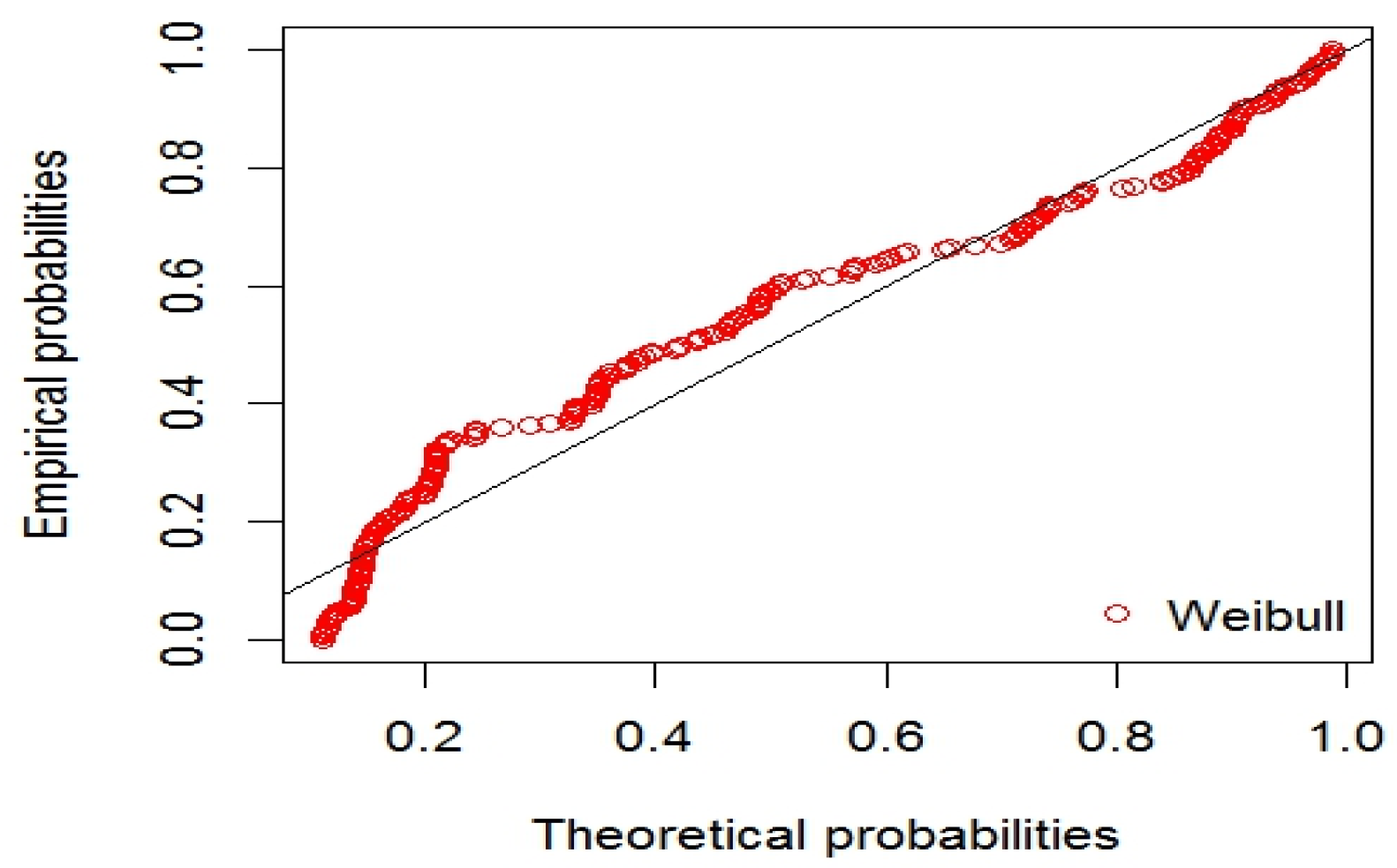
The cumulative distribution function (CDF) of GEVD is given by

$$F(x)=\{\begin{array}{cc}{e}^{-{(1-\mathrm{k}\frac{x-\xi }{\alpha })}^{1/k}};& k\ne 0\\ e^{-e^{-\frac{x-\xi }{\alpha }}};& k=0\end{array}.$$

(6)

Variable X is bounded by $(\xi +\alpha )/k$ from above, if $k>0$ and from below if $k<0$, where $\xi \in R$ and $\alpha >0$. We have three cases of this distribution as

• Weibull distribution ($k>0$),
• Ferechet distribution ($k<0$),
• Gumbel distribution ($k=0$).

We now want to check the heavy tail property. Using the ii and iii criteria, it is observed that the Ferechet-Weibull distribution and the Weibull distribution with $0<\beta <1$ have a heavy tail. However, based on the v criterion, the Gumbel distribution does not have the heavy tail property.

4.1.2. Pareto Distribution

The Pareto distribution is a skewed, heavy-tailed distribution that is sometimes used to model the distribution of incomes. This distributional model is important in applications because many datasets are observed to follow a power law probability tail, at least approximately, for large values of x. Stable distributions with index $\alpha$ are also asymptotically Pareto in their probability tails, and this fact has been frequently used to develop estimators for those distributions. The CDF of Pareto is given by

$$F(x)=1-{\left(\frac{\alpha }{x+\alpha }\right)}^k;x>0.$$

(7)

The hazard function of the Pareto distribution, $\frac{k}{x+\alpha }$, is a decreasing function for positive values of k and $\alpha$. Thus, using the ii and iii criteria, it has a heavy tail.

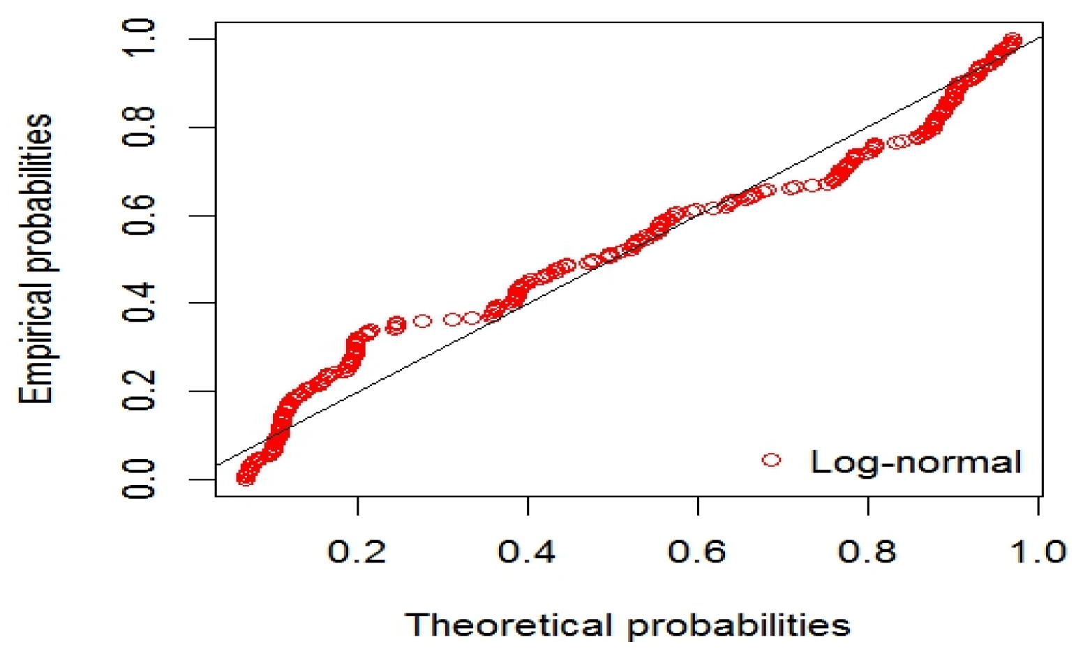
4.1.3. Log-Normal Distribution

A log-normal distribution is applied as the standard model for financial data. It is used in many different fields of study, such as economics, metrology, biology, neuroscience and engineering. The density function of a log-normal distribution, with shape parameter $\sigma >0$ and scale parameter $\mu >0$ is

$$f(x)=\frac{1}{\sqrt{2\pi }x\sigma }{e}^{-\frac{1}{2}{(\frac{\ln x-\ln \mu }{\sigma })}^2};x>0.$$

(8)

The tail heaviness property of the log-normal distribution depends on the variance. In other words, based on the iv criterion, we can write,

$$\varpi =\frac{Var(X)}{E{(X)}^2}=e^{{\sigma }^2}-1.$$

(9)

The $\varpi$ is longer than 1, if $\sigma >0.8226$ or $\sigma <0.8226$.

4.1.4. Burr Type XII Distribution

Burr [24] introduced twelve cumulative distribution functions with the primary purpose of fitting distributions to real data. One of the most important of them is the Burr Type XII distribution. The cumulative distribution function of the Burr Type XII is given by

$$F(x)=1-{(1+x^{\beta })}^{-\alpha };x>0.$$

(10)

Here, $\alpha >0$ and $\beta >0$ are the two shape parameters. The shape of the hazard rate function of the Burr Type XII distribution depends only on parameter $\beta$. Its capacity to assume various shapes often permits a good fit when used to describe biological, financial, engineering or other experimental data. It also approximates the distributional form of normal, log-normal, gamma, logistic, and several Pearson-type distributions. For instance, the normal density function may be approximated as a Burr Type XII distribution with $\beta$ = 4.8544 and $\alpha =6.2266$ and the gamma distribution with shape parameter 16 can be approximated as a Burr Type XII distribution with $\beta$ = 3 and $\alpha$ = 6, and the log-logistic distribution is a special case of the Burr Type XII distribution. In addition, using the i, ii and iii criteria, it is observed that the Burr Type XII has a heavy tail.

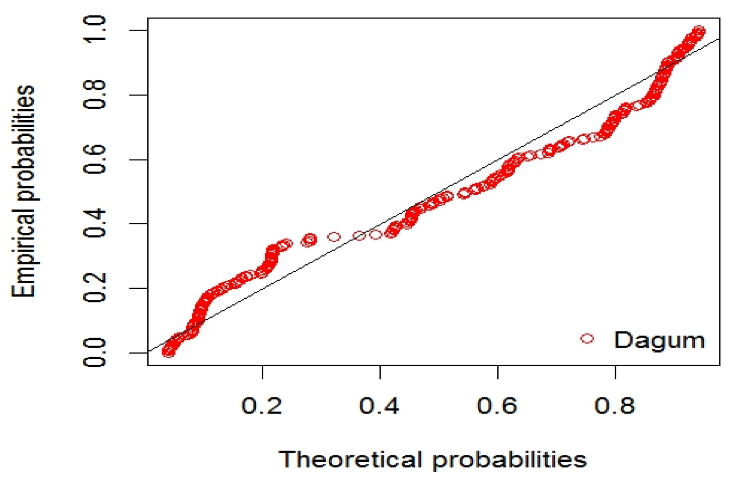
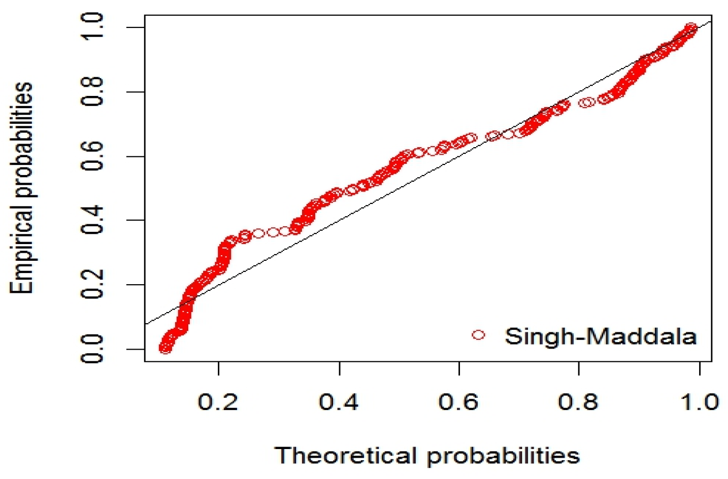
4.1.5. Dugum and Singh-Maddala Distribution

The Dugum and Singh-Maddala distributions are the special case of the generalized Beta kind 2 (GB₂) distribution. The CDFs of these distributions are given by, respectively:

$$F(x)={\left(1+{(\frac{\beta }{x})}^{\alpha }\right)}^{-\gamma };x>0,$$

(11)

and

$$F(x)=1-{\left(1+{(\frac{x}{\beta })}^{\alpha }\right)}^{-\gamma };x>0,$$

(12)

Here, all three of the parameters are positive. In addition, the r^th moment of these distributions can be written as

$$E(X^r)=\frac{{\beta }^r}{(\gamma -1)!}\Gamma (\frac{r}{\alpha }+1)\Gamma (1-\frac{r}{\alpha })$$

and

$$E(X^r)={\beta }^r\gamma B(\frac{r}{\alpha }+\gamma ,1-\frac{r}{\alpha }),$$

where $\Gamma (.)$ and $B(.,.)$ denote the Gamma distribution and the Beta distribution, respectively. Using the i criterion, it is observed that the moments of these distributions only exist for values of $-\gamma \alpha <r<\alpha$. It indicates that these distributions have potentially tail heaviness properties.

5. Application of the NMST of Tehran Stock Exchange

In this section, the data set of daily returns of the top 30 companies from the Tehran Stock Exchange indices was used to study the performance of the proposed model selection test. All the programs are written in R. The mean, standard deviation, skewness and kurtosis of this data are 2.937687, 0.261701, 0.273005 and 1.790659, respectively. It is observed that the skewness and kurtosis are not close to zero and three, respectively. Thus, the data set has a higher peak, fatter tail and skewness in comparison to the Normal distribution. For more study, we demonstrate how it deviates from the Normal distribution using the Shapiro-Wilk (S-W) test, Kolmogrov-Smirnov (K-S) test, Anderson-Darling (A-D) test and Jarque-Bera (J-B) test. For each test, the null hypothesis is that the data are normally distributed. If the p-value is less than the significant level (0.05) of the given hypothesis, the null hypothesis will be rejected. For computing the mentioned test, we use the nortest and tseries in the R package. The results are provided in

Table 1. Different Normality tests for the proposed data.

	S-W	K-S	A-D	J-B
Value of test	0.4659	0.2957	6.0576	953.5819
p-value	9.605 × 10−11	2.493 × 10−9	3.471 × 10−15	<2.2 × 10−16

S-W: Shapiro-Wilk test; K-S: Kolmogrov-Smirnov test; A-D: Anderson-Darling test; J-B: Jarque-Bera test.

. Based on Table 1, we observe that the data do not follow the Normal distribution. Thus, we use the heavy-tailed distribution for modeling the data. First, we check the adequacy of the Weibull (We) distribution, Pareto (Pa) distribution, Burr Type XII (BXII) distribution, log-normal (LN) distribution, Dagum (Da) distribution and Singh-Maddala (S-M) distribution using three different well-established model selection criteria such as K-S minimum distance criterion, Akaike information criterion ($AIC=-2{\displaystyle \sum _{i=1}^{n}lo}g{f}^{{\widehat{\alpha }}_n}(x_i)+2p$), Bayesian information criterion ($BIC=-2{\displaystyle \sum _{i=1}^{n}lo}g{f}^{{\widehat{\alpha }}_n}(x_i)+p\log n$) and maximum log-likelihood criterion (LL). We select the best model among all competitive distributions that has the smallest AIC, BIC and K-S distance and the greatest LL values. We first estimate the unknown parameters using MLEs. The results are presented in

Table 2. Estimated parameters, AIC values, BIC values and log-likelihood values for different distribution functions.

Models	Parameters	MLE	AIC	BIC	LL
We	$\alpha$	12.07339	64.83431	71.86922	−30.41716
	$\beta$	3.059887
Pa	$\alpha$	5037634	1038.656	1045.691	−517.3281
	k	1715197
BXII	$\alpha$	0.071667	1072.124	1079.159	−534.0619
	$\beta$	12.98343
LN	mean	1.073703	36.6373	43.67221	−16.31865
	s.d.	0.088294
Da	$\alpha$	13.39737	36.8876	47.43996	−17.4438
	$\beta$	2.142820
	$\gamma$	37.14274
S-M	$\alpha$	12.22984	66.50122	77.05358	−30.25061
	$\beta$	4.134818
	$\gamma$	40.52715

MLE: maximum likelihood estimator; AIC: Akaike information criterion; BIC: Bayesian information criterion; LL: maximum log-likelihood criterion.

. It is clear that the Da and LN distributions have comparatively better fitting for the present data set. The We and S-M distributions also have a good fit. We provide the Probability-Probability (P-P) plots for different distributions in Figure 1, Figure 2, Figure 3, Figure 4, Figure 5 and Figure 6. Moreover, the empirical survival function and the fitted survival functions are presented in Figure 7. Therefore, based on Figure 1, Figure 2, Figure 3, Figure 4, Figure 5, Figure 6 and Figure 7, it is observed that the BXII and Pa distributions do not fit the data reasonably well, and hence, they cannot be used to obtain inferential results from the considered data set. Using different model selection criteria, we can compare the proposed distributions. However, these criteria have some disadvantages. For example, the LL criterion assumes that the number of parameters in each competitive model is the same. In addition, one problem with AIC and BIC are that their values have no intrinsic meaning; in particular, AIC and BIC are not invariant to a one-to-one transformation of the random variables and values of AIC and BIC depend on the number of observations. Thus, we consider the NMST for comparing the heavy-tailed distributions.

Now, we check the results using the proposed interval for model selection. We consider four cases of rival models as:

(1)

Da (f) and LN (g),

(2)

Da (f) and We (g),

(3)

We (f) and S-M (g),

(4)

Da (f) and S-M (g).

Based on the estimated values, we construct the proposed interval. This interval for the above four cases are (1.9878339, 2.0104310), (−2.748678, −2.614607), (−4.2395868, −4.1287672) and (−172.43378, −161.83113), respectively. For Case 1, it is observed that both limits of the tracking interval are positive, which indicates that the LN is better than the Da distribution to estimate the true model for this data. However, the length of this interval is small, so we can conclude that the two models are similar to estimate the true model (as expected). For Cases 2–4, both limits of the tracking interval are negative, so the model (f) is better than the model (g). It is observed that this interval selects the correct model well. In addition, computational steps of this interval are simple. Now, we suppose that some of the data are missed (censored). We generate artificially left censored data from the data set as

• Scheme 1: $n=249,c=5$ (The first 5 pieces of data are not observed).
• Scheme 2: $n=249,c=20$ (The first 20 pieces of data are not observed).
• Scheme 3: $n=249,c=80$ (The first 60 pieces of data are not observed).

Here, n is the complete sample size and c is the number of the left censored data. Based on Case 1, the proposed intervals for Schemes 1–3 are (1.952583, 2.036342), (1.974464, 2.060377) and (2.141464, 2.212098), respectively. Similarly, for Case 2, the intervals are (−2.757090, −2.620894), (−2.768494, −2.623881) and (−2.680060, −2.497014), respectively. For Case 3, the results are (−4.246638, −4.134079), (−4.264661, −4.145781) and (−4.304638, −4.144865), respectively, and for Case 4, the proposed intervals are (−171.1225, −160.5491), (−167.1976, −156.6924) and (−148.70633, −139.26066), respectively. It is observed that the results are similar to the complete data.

6. Conclusions

The heavy-tailed distributions are the most important distributions in several applied sciences such as economics, financial engineering and mathematical finance. Moreover, in many situations, we cannot observe the complete information about the data. In this situation, the problem of choosing the correct distribution becomes more difficult. There are different criteria such as AIC, BIC, LL and K-S distance for comparing the models. These criteria have some disadvantages. Thus in this paper, we have proposed a new model selection test for comparing the heavy-tailed distributions under complete and censored data. This interval enlightens the unavoidable variability of any criterion based on log-likelihood ratio such as AIC, BIC and their variants. Based on this test, we can make the best possible decision based on whatever data are available at hand. The computational steps of NMST are easy to compute and could be very useful for censored data. We hope that the new model selection test will attract wider application in all areas of research.

References

1. S. Ahna, H.T. Kim Joseph, and V. Ramaswami. “A new class of models for heavy tailed distributions in finance and insurance risk.” Insur. Math. Econ. 51 (2012): 43–52. [Google Scholar] [CrossRef]
2. K. Burnecki, A. Wylomanska, and A. Chechkin. “Discriminating between light- and heavy-tailed distributions with limit theorem.” PLoS ONE 10 (2015): e0145604. [Google Scholar] [CrossRef] [PubMed]
3. X. Hao, and Q. Tang. “Asymptotic ruin probabilities for a bivariate Leavy-driven risk model with heavy-tailed claims and risky investments.” J. Appl. Probab. 49 (2012): 939–953. [Google Scholar]
4. G. Pastor, I. Mora-Jiménez, J. Caamaño Antonio, and R. Jäntti. “Asymptotic expansions for heavy-tailed data.” IEEE Signal Process. Lett. 23 (2016): 444–448. [Google Scholar] [CrossRef]
5. O.E. Barndor-Nielsen. “Superposition of Ornstein-Uhlenbeck type processes.” Theory Probab. Appl. 45 (2001): 175–194. [Google Scholar] [CrossRef]
6. S.R. Chandra, D. Mukherjee, and I. SenGupta. “PIDE and solution related to pricing of levy driven arithmetic type floating Asian options.” Stoch. Anal. Appl. 33 (2015): 630–652. [Google Scholar] [CrossRef]
7. I. Sen Gupta. “Generalized BN-S stochastic volatility model for option pricing.” Int. J. Theor. Appl. Financ. 19 (2016): 1650014. [Google Scholar] [CrossRef]
8. O.E. Barndor-Nielsen, and N. Shephard. “Non-Gaussian Ornstein-Uhlenbeck based models and some of their uses in financial economics.” J. R. Stat. Soc. Ser B 63 (2001): 167–241. [Google Scholar] [CrossRef]
9. D. Kundu, R.D. Gupta, and A. Manglick. “Discriminating between the log-normal and generalized exponential distribution.” J. Stat. Plan. Inference 127 (2005): 213–227. [Google Scholar] [CrossRef]
10. A.K. Dey, and D. Kundu. “Discriminating among the Log-Normal, Weibull and Generalized Exponential distributions.” IEEE Trans. Reliab. 58 (2009): 416–424. [Google Scholar] [CrossRef]
11. D.R. Cox. “Test of Separate Families of Hypothesis.” In Proceedings of the Fourth Berkeley Symposium on Mathematical Statistics and Probability, Statistical Laboratory of the University of California, Berkeley, CA, USA, 20 June–30 July 1960; pp. 105–123.
12. Q.H. Vuong. “Likelihood ratio tests for model selection and non-nested hypothesis.” Econometrica 57 (1989): 307–333. [Google Scholar] [CrossRef]
13. Q.H. Vuong, and W. Wang. “Minimum chi-square estimation and tests for model selection.” J. Econom. 56 (1993): 141–168. [Google Scholar] [CrossRef]
14. D. Commenges, B. Liquet, and C. Proust-Lima. “Choice of prognostic estimators in joint models by estimating differences of expected conditional Kullback-Leibler risks.” Biometrics 68 (2012): 380–387. [Google Scholar] [CrossRef] [PubMed]
15. H. Panahi, and S. Asadi. “A model selection test with application to the censored data of carbon nanotubes coating.” Prog. Color Colorants Coat. 9 (2016): 17–28. [Google Scholar]
16. H. Panahi, and A. Sayyareh. “Parameter estimation and prediction of order statistics for the Burr Type XII distribution with Type II censoring.” J. Appl. Stat. 41 (2014): 215–232. [Google Scholar] [CrossRef]
17. H. Panahi, and A. Sayyareh. “Estimation and prediction for a unified hybrid-censored Burr Type XII distribution.” J. Stat. Comput. Simul. 86 (2016): 55–73. [Google Scholar] [CrossRef]
18. H. Panahi, and A. Sayyareh. “Tracking interval for type II hybrid censoring scheme.” JIRSS 13 (2014): 187–208. [Google Scholar]
19. K.C. Cain, S.D. Harlow, R.J. Little, B. Nan, M. Yosef, J.R. Taffe, and M.R. Elliott. “Bias due to left truncation and left censoring in longitudinal studies of developmental and disease processes.” Am. J. Epidemiol. 25 (2011): 1–7. [Google Scholar] [CrossRef] [PubMed]
20. S. Mitra, and D. Kundu. “Analysis of left censored data from the generalized exponential distribution.” J. Stat. Comput. Simul. 78 (2008): 669–679. [Google Scholar] [CrossRef]
21. U. Singh, and A. Kumar. “Bayesian estimation of the exponential parameter under a multiply type-II Censoring scheme.” Aust. J. Stat. 36 (2007): 227–238. [Google Scholar]
22. E.M. Thompson, J.B. Hewlett, L.G. Baise, and R.M. Voge. “The Gumbel hypothesis test for left censored observations using regional earthquake records as an example.” Nat. Hazards Earth Syst. Sci. 11 (2011): 115–126. [Google Scholar] [CrossRef] [Green Version]
23. T.A. Louis. “Finding the observed information matrix when using the EM algorithm.” J. R. Stat. Soc. Ser. B 44 (1982): 226–233. [Google Scholar]
24. I.W. Burr. “Cumulative frequency functions.” Ann. Math. Stat. 13 (1942): 215–232. [Google Scholar] [CrossRef]
25. H. Panahi, and A. Sayyareh. “Tracking interval for doubly censored data with application of plasma droplet spread samples.” J. Stat. Res. Iran 11 (2015): 147–176. [Google Scholar] [CrossRef]
26. H. Cramér. Mathematical Methods of Statistics. Princeton, NJ, USA: Princeton University Press, 1946. [Google Scholar]
Figure 1. The Probability-Probability (P-P) plot for Dagum distribution.
Ijfs 04 00024 g001
Figure 2. The P-P plot for Singh-Maddala distribution.
Ijfs 04 00024 g002
Figure 3. The P-P plot for log-normal distribution.
Ijfs 04 00024 g003
Figure 4. The P-P plot for Weibull distribution.
Ijfs 04 00024 g004
Figure 5. The P-P plot for Pareto distribution.
Ijfs 04 00024 g005
Figure 6. The P-P plot for Burr XII distribution.
Ijfs 04 00024 g006
Figure 7. Empirical survival function and the fitted survival functions.
Ijfs 04 00024 g007